MARINE ECOLOGY PROGRESS SERIESMar Ecol Prog Ser

Vol. 395: 201–222, 2009doi: 10.3354/meps08402

Published December 3

INTRODUCTION

The concept of acoustic interference is familiar toanyone who has tried to have a conversation in a noisyrestaurant or to listen for the ring of a phone in anotherroom through the acoustic clutter from a nearby televi-sion. In such situations the collective noise from manysources or the clutter of voices coming from a singlelocation may impede one’s ability to understand, rec-

ognize or even detect sounds of interest. This type ofacoustic interference is referred to as masking andresults in the reduction of a receiver’s performance, asthe sound of interest cannot be effectively perceived,recognized or decoded. In the case of 2-way communi-cation involving a sender and a receiver, maskingresults in the reduction of both the sender’s and thereceiver’s performance; a phenomenon we will refer tohere as communication masking.

© Inter-Research 2009 · www.int-res.com*Email: cwc2@cornell.edu

Acoustic masking in marine ecosystems: intuitions, analysis, and implication

Christopher W. Clark1,*, William T. Ellison2, Brandon L. Southall3, 4, Leila Hatch5, Sofie M. Van Parijs6, Adam Frankel2, Dimitri Ponirakis1

1Bioacoustics Research Program, Cornell Laboratory of Ornithology, 159 Sapsucker Woods Road, Ithaca, New York 14850, USA2Marine Acoustics, 809 Aquidneck Avenue, Middletown, Rhode Island 02842, USA

3Southall Environmental Associates, 911 Center Street, Suite B, Santa Cruz, California 95060, USA4Long Marine Laboratory, University of California, Santa Cruz, 100 Shaffer Road, Santa Cruz, California 95060, USA

5Gerry E. Studds Stellwagen Bank National Marine Sanctuary, NOAA, 175 Edward Foster Road, Scituate, Massachusetts 02066, USA

6 NOAA Fisheries, Northeast Fisheries Science Center, 166 Water Street, Woods Hole, Massachusetts 02543, USA

ABSTRACT: Acoustic masking from anthropogenic noise is increasingly being considered as a threatto marine mammals, particularly low-frequency specialists such as baleen whales. Low-frequencyocean noise has increased in recent decades, often in habitats with seasonally resident populations ofmarine mammals, raising concerns that noise chronically influences life histories of individuals andpopulations. In contrast to physical harm from intense anthropogenic sources, which can have acuteimpacts on individuals, masking from chronic noise sources has been difficult to quantify at individ-ual or population levels, and resulting effects have been even more difficult to assess. This paper pre-sents an analytical paradigm to quantify changes in an animal’s acoustic communication space as aresult of spatial, spectral, and temporal changes in background noise, providing a functional defini-tion of communication masking for free-ranging animals and a metric to quantify the potential forcommunication masking. We use the sonar equation, a combination of modeling and analytical tech-niques, and measurements from empirical data to calculate time-varying spatial maps of potentialcommunication space for singing fin (Balaenoptera physalus), singing humpback (Megopteranovaeangliae), and calling right (Eubalaena glacialis) whales. These illustrate how the measured lossof communication space as a result of differing levels of noise is converted into a time-varying mea-sure of communication masking. The proposed paradigm and mechanisms for measuring levels ofcommunication masking can be applied to different species, contexts, acoustic habitats and oceannoise scenes to estimate the potential impacts of masking at the individual and population levels.

KEY WORDS: Communication masking · Ambient noise · Acoustic habitat · Communication space ·Spatio-temporal variability · Spectral variability · Cumulative effects · Marine mammals · Baleen whales

Resale or republication not permitted without written consent of the publisher

OPENPEN ACCESSCCESS

Contribution to the Theme Section ‘Acoustics in marine ecology’

Mar Ecol Prog Ser 395: 201–222, 2009

The term masking was borrowed by analogy fromvision and in general refers to the failure by a person torecognize the occurrence of one type of stimulus as aresult of the interfering presence of another stimulus.Auditory masking was first empirically measured andquantified by experiments testing a listener’s ability tohear a test tone in the presence of noise (Tanner 1958).In humans, masking is the amount (or process) bywhich the audibility threshold for one sound is raisedby the presence of another sound (Moore 1982, p 74).

Early masking studies in humans showed that tonalsignals are most effectively masked by tonal sounds orbroadband noise with frequencies similar to the sig-nal’s frequency (Wegel & Lane 1924, Fletcher 1940).Further studies revealed that this basic principle ofmasking applies to non-human mammals as well(Scharf 1970, Fay 1988). These observations along withadditional evidence suggest that the mammalian audi-tory system segregates an incoming acoustic signalinto its constituent frequencies, leading to optimizationof signal-to-noise ratio and parallel processing of theharmonic components of complex sounds (Moore 1982,Fay 1992, Niemiec et al. 1992).

There are 2 major, but not necessarily exclusive, cat-egories of masking: energetic masking and informa-tional masking (Ihlefeld & Shinn-Cunningham 2008,Yost et al. 2008). Traditional energetic masking refersto the case when the masking sound contains energyin the same frequency band and occurs at the sametime as the signal of interest, such that the signal isinaudible. In contrast, informational masking is consid-ered to operate further along in the auditory processand occurs when the signal is still audible but cannotbe disentangled from a sound with similar characteris-tics (Watson 1987, Brungart 2004). Most of us are famil-iar with both energetic and informational masking,and have experienced situations which involved mix-tures of both forms.

There has been substantial research on the effects ofnoise on human hearing and speech communication(e.g. Pearsons et al. 1977, Nilsson et al. 1994; forreviews see Kryter 1994, Miller 1997, Yost 2000), con-centration and cognitive functions (e.g. general‘annoyance’), and physiological functions, includingstress responses (e.g. Schultz 1978, Beranek & Ver1992, Tafalla & Evans 1997, Evans 2001). Theseimpacts can occur in environments with persistent lev-els of elevated ambient noise, such as under industrialwork conditions, where chronic exposure can result inhearing loss (Kryter 1994). Such physiological effects,although not considered communication masking inthe traditional sense of the term, can result in the lossof one’s ability to detect important sounds. Addition-ally, studies have been conducted on how people usesound as a means of sensing the acoustic ‘scene’ in a

spatial manner analogous to visual field perception(Bregman 1990), as well as on the longer-term andlarger-scale deleterious effects of the noise environ-ment on human development and behavior (e.g. Evans2001, 2003). For marine mammals, Richardson et al.(1995) presented an excellent overview and outline ofnoise masking, while recognizing the inherent difficul-ties of quantifying the potential effects. The analyticalparadigms arising from these and other studies pro-vide a useful starting framework by which to explorethe effects of noise on marine animals (e.g. Southall etal. 2007).

Masking in a broad sense is a key concern regardingthe non-injurious impact of interfering sound on marinewildlife, and the potential for communication maskingis the aspect most often associated with long-term ef-fects of anthropogenic sound. That noise from anthro-pogenic sources might affect marine mammal commu-nication was first articulated by Payne & Webb (1971),who proposed that the collective, very low frequencynoise (<100 Hz) from ocean shipping might reduce therange over which blue (Balaenoptera musculus) and fin(B. physalus) whales are able to communicate. Thesewhales are members of a remarkable group of marinemammals that have adapted to an aquatic existenceover tens of millions of years (see Reynolds & Rommel1999). During this evolutionary period, marine mam-mals evolved many ingenious mechanisms for produc-ing, receiving and using sound for a variety of biologi-cal functions (e.g. Schusterman 1981, Clark 1990, Au1993, Richardson et al. 1995, Tyack 1998, Wartzok &Ketten 1999, Clark & Ellison 2004).

Different groups of marine mammals appear to betuned to different frequency bands, despite being gen-erally quite similar in how they hear in the presence ofinterfering noise, and having ears that appear to be fun-damentally similar in structure and function. Recently,Southall et al. (2007) suggested using an ‘M-weighting’function1 as an appropriate method to account for amarine mammal’s auditory sensitivity in assessingpotential impacts of exposure to high-level sounds. Forbaleen whales, Richardson et al. (1995) and Clark &Ellison (2004) deduced that low-frequency auditorythresholds are very likely ambient noise limited. Con-sequently, these low-frequency specialists will be dis-proportionately affected by changes in low-frequencynoise levels and thus particularly susceptible to themasking effects of noise on their communication sig-nals. It is likely that acoustic masking by anthropogenicsounds is having an increasingly prevalent impact onanimals’ access to acoustic information that is essential

202

1Derived for different marine mammal ‘functional hearinggroups’ and in a manner based on the C-weighting functionused in humans.

Clark et al.: Acoustic masking in marine ecosystems

for communication and other important activities suchas navigation and prey/predator detection. In an evolu-tionary time frame relevant to species adaptations,these impacts are essentially immediate. Developing acritical and extensive understanding of these issues willrequire a broad-based, rigorous and quantitative ap-proach that better identifies the underlyingrelationships, factors, and variables.

There has been an increasing level of discussion anddebate over how marine mammals may be affected byanthropogenic noise in the ocean (see NRC 2000, 2003,2005, Cox et al. 2006, Southall et al. 2007), with mostattention directed at understanding the physiologicaland behavioral impacts from short-term, small-scale,high intensity exposures (i.e. acute). There is recogni-tion that long-term, large-scale (i.e. chronic), lowintensity noise exposures might also be affecting indi-viduals and populations, and communication maskingis often mentioned or implied as a probable mecha-nism (Payne & Webb 1971, Richardson et al. 1995, NRC2000, 2003, Southall 2005, Nowacek et al. 2007, Hatchet al. 2008). Richardson et al. (1995) outlined the basiccomponents for, and a few models have been createdto estimate, the spatial extent of communication mask-ing. One such model for beluga whales Delphi-napterus leucas considered the physical environmentas well as both the acoustic behavior and hearing abil-ity of the animal (Erbe & Farmer 2000). Nevertheless,there has not yet been an overarching paradigm forevaluating or measuring, in a realistic spatial sense,the potential impacts (either short- or long-term) fromcommunication masking on free-ranging animals.

Here we consider acoustic communication maskingin the marine environment with particular attention toa major group of marine mammals, the mysticetes, dueto their low-frequency vocalization range and theubiquitous growth in oceanic noise in this same range(Andrew et al. 2002, McDonald et al. 2006). We enu-merate a number of key concepts such as acoustichabitat, acoustic scene, acoustic space and acousticecology to expand on some previous syntheses andrecent research (e.g. Richardson et al. 1995, Clark &Ellison 2004, Southall et al. 2007, Hatch et al. 2008). We

introduce the concept of a dynamic spatio-spectral-temporal acoustic habitat, and use this perspective todevelop analytical representations by which to studythe masking effects of noise on acoustic communica-tion. We formalize a protocol that integrates a form ofthe sonar equation (Urick 1983) with biological know-ledge to quantify the effects of an actual movinganthropogenic noise source on the area over which asingle animal’s acoustic communication signal mightbe recognized by a uniformly distributed set of con-specifics. The result is standardized by referencingthat area to the ambient noise conditions withoutanthropogenic sources to yield a time-varying maskingindex. This procedure for a single, stationary callinganimal in a time-varying acoustic scene is thenexpanded to a population of stationary calling animalsto quantify variability of communication maskingthroughout a habitat region. Furthermore, we general-ize the algorithm to include multiple noise sources andthereby formalize a method for quantifying the cumu-lative effects of co-varying numbers and types ofanthropogenic sources.

Background

A broad consideration of acoustic masking mustinclude the masking of conspecific communications, aswell as the masking of other biologically importantsounds (e.g. echolocation sounds for foraging andsounds from predators) and abiotic sound cues (e.g.sounds from a distant shoreline, earthquakes, volumereverberation). Furthermore, we must consider bothshort-term, proximate effects (e.g. the temporaryinability of an animal to hear the communication callsof a conspecific) as well as long-term, ultimate effects(e.g. decreased survivorship and fecundity as a resultof the persistent degradation of an acoustic habitatover an animal’s lifetime).

A central concept is the effective 3-dimensionalspace over which bioacoustic activity occurs (‘bio-acoustic space’). Some of the most common types(Table 1) include the space over which (1) sounds from

203

Receiver Sound sourceSelf Conspecific Other species Abiotic

Self Echolocation: navigation Communication Predator avoidance, Navigation, and food finding food finding food finding

Conspecific Communication Eavesdropping, bi-static navi- NA Bi-static gation, bi-static food finding navigation

Other species Detection by predator Bi-static food finding Eavesdropping NA

Table 1. Matrix listing different types of acoustic spaces that can be affected by noise masking. NA: not applicable

Mar Ecol Prog Ser 395: 201–222, 2009

an individual animal can be heard by other con-specifics, or a listening animal can hear sounds fromother conspecifics (i.e. ‘communication space’ or ‘bi-static space’); (2) an individual animal can hear bio-acoustic signals from itself (i.e.‘ echolocation’ or ‘echo-ranging space’); (3) an individual animal can hearsounds from interacting conspecifics (i.e. ‘eavesdrop-ping space’); (4) an individual animal can hear biologi-cally relevant signals from animals other than con-specifics (i.e. ‘predator space’); (5) an individual animalcan hear biologically relevant food resource cues (i.e.‘volume reverberation space’); and (6) an individualanimal can hear physically relevant sound cues fromoceanographic features (i.e. ‘reverberation space’,‘internal wave space’)2. At any one time an individualanimal has multiple acoustic spaces, some dominatedby factors operating within the biological, evolutionarydomain (e.g. receiver characteristics including hearingabilities as well as source level, directivity, and fre-quency band of a calling conspecific) and some domi-nated by physical factors operating outside of an evo-lutionary domain (e.g. water depth, sound velocityprofile, substrate composition, backscatter), and someof which are co-dependent and co-varying.

We define ‘communication space’ as the volume ofspace surrounding an individual, within whichacoustic communication with other conspecifics can beexpected to occur. It is similar to ‘active space’ (e.g.Brenowitz 1982, Janik 2000), but here we expand onthis concept with regard to acoustic communication.The size and shape of any particular bioacoustic spaceis influenced by multiple factors which vary differentlyover time. For example, the communication space of acaller will vary considerably depending on a host ofvariables relating to both sender and receiver, includ-ing source level, directivity, and orientation; soundtransmission path conditions; ambient noise; andreceiver orientation and detection capabilities. Thevalues of these factors and their combinations will varyfor different bioacoustic spaces and different species.For example, an animal’s echolocation space is likelyto be smaller than its communication space becausethe transmission loss for the echoing signal at a givendistance is twice that for a communication signal; thiswould be even more so if the echolocation signal ismuch higher in frequency than the communication sig-nal, and thus subject to additional scattering andabsorption losses. Likewise, the communication space

of a pilot whale whistling in the 7–15 kHz frequencyband will be much smaller than the communicationspace of a fin whale calling in the 30–80 Hz band, evenif the output levels are similar, as a result of physicalacoustics. While communication space has not beenextensively studied in animals, some interesting calcu-lations and estimates have been made for red-wingedblackbirds Agelaius phoeniceus (Brenowitz 1982),bowhead whales Balaena mysticetus (Richardson etal. 1995), blue monkeys Cercopithecus mitis and grey-cheeked mangabees Cercocubus albigena (Brown1989), yellowfin tuna Thunnus albacares (Finneran etal. 2000), bottlenose dolphins (Tursiops truncatus(Janik 2000), and northern elephant seals Miroungaangustirostris (Southall et al. 2003).

204

CR Communication rangeCS Communication space (km2)DI Directivity index (dB)DT Detection threshold (dB)ƒ0 Mean or center frequency (Hz)Leq Equivalent level (dB)M Communication masking indexNL Noise band level (dB re 1 µPa) at a receiver, i.e.

the sum of ambient noise and noises fromspecific sources with distinctive spatial andtemporal parameters

NSL Noise source level (dB)NTL Noise transmission loss (dB)PCS Potential communication space (km2)PR Probability of recognitionPSD Power spectral densityR0 Range between source and receiver (m)RD Recognition differential (dB)RINT Range interval (m)RL Received level of sound at a receiver (dB)rms Root mean squareS SenderSBNMS Stellwagen Bank National Marine SanctuarySE Signal excess (dB)SEL Sound energy level (dB re 1 µPa2 s)SG Signal processing gain (dB)SL Source level of sound as emitted with reference

to a 1 m distance, dB re 1 µPa @ 1 mSNR Signal-to-noise ratio (since this is a ratio there is

no reference unit)SPL Sound pressure level (dB)SRD Source-receiver depth (m), depth of calling and

receiving whalesT Duration (s)TL One way transmission loss between sound

source and receiver inclusive of spreading losses,refraction, scattering, absorption and otherboundary losses (dB). We use the KRAKENmodel to calculate TL (Porter & Reiss 1985)

W Bandwidth (Hz)ρc Acoustic impedance

Table 2. List of abbreviations

2There are cases where information is available to an animalvia the acoustic channel from the combination of a bioacousticsignal and the effects of sound propagation on that signal, forexample the multi-modal arrivals of a communication call(Premus & Spiesberger 1997). We recognize but do not con-sider these other cases here.

Note:

The units for SNRand TL were

corrected afterpublication

Clark et al.: Acoustic masking in marine ecosystems

In the following section we translate the concept ofacoustic space as outlined above into a series of math-ematical expressions based on a family of sonar equa-tions. We use this modeled approach as the frameworkby which to quantify the masking effects of ambientnoise and specific sound sources on communicationspace. We provide examples of communication mask-ing due to shipping noise for 3 mysticete whale spe-cies. A solution for cumulative impact from multiplenoise sources is achieved by generalizing the algo-rithm, and the resultant metric is standardized by ref-erence to the amount of communication space thatwould have been available under what we define asancient ambient noise conditions.

METHODOLOGY

A model of communication masking must includethe basic elements of source characteristics, acousticpropagation and received sound exposure, with theresult cast in metrics that provide a methodology forassessing the relative effects of communication mask-ing on the animal’s bioacoustic space. The key ele-ments in the model must at least extend from thenoise(s) and/or sound(s) experienced by the animalthrough the initial stages of the animal’s auditoryprocesses when the sound of interest is recognized.Table 2 lists terms and abbreviations used.

Examples

Fig. 1 shows 24 h spectrograms based on acousticdata collected with similar recorders in 2 differenthabitats with known populations of fin whales; Fig. 1A

is from the Gulf of California, a habitat with low back-ground noise conditions, while Fig. 1B is from theMediterranean Sea, a habitat with high backgroundnoise conditions (Clark et al. 2002, Croll et al. 2002).Fin whales were singing in both habitats and are veryevident in the Baja California habitat (Fig. 1A), butbarely evident in the Mediterranean habitat which isdominated by shipping noise (Fig. 1B).

In Fig. 2, we convert those data into quantile statis-tics for the power spectral density (PSD) distribution.For the Gulf of California habitat (Fig. 2A), this revealsa dominant 20 Hz peak representing the collectivevoices of fin whale singers, while for the Mediterra-nean habitat (Fig. 2B) there is no apparent 20 Hz peak,and the contribution of singers to the spectral energydistribution is hidden within a broader, 15–80 Hz bandof noise. Thus fin whale singers in the Gulf of Califor-nia are not masked by noise in their communicationband (18–28 Hz), while band level noise in the Medi-terranean Sea, at least for this 24 h period, is so highthat singers might have a problem being heard byother fin whales. Conversion of these kinds of acousticscenes into measures of communication maskingrequires careful consideration and inclusion of vari-ability in the temporal, spectral and spatial dimensionsof the acoustic environment at biologically meaningfulresolutions. That is, the temporal resolution of theanalysis should match the durations of the sounds pro-duced and perceived by the species of concern, just asthe spectral resolution should be matched to the fre-quency bands in which the species communicates, andthe spatial resolution should be matched to an areaover which the animal communicates.

An example of adjusting spectral resolutions tomatch the frequency characteristics of species-specificwhale sounds may be seen in recent data collected

205

Fig. 1. Examples of 24 h acoustic scenes for 2 habitats in which male fin whales were singing: (A) Gulf of California and (B)Mediterranean Sea (2 kHz sampling rate, 1024 pt FFT, 50% overlap, Hanning window). Both recorders were similar with flat

(±1.0 dB) frequency response between 10 and 585 Hz. Scale bar indicates rms pressure level in dB re 1 µPa

Mar Ecol Prog Ser 395: 201–222, 2009

from an autonomous seafloor recorder inthe Stellwagen Bank National MarineSanctuary (SBNMS), an area with knownseasonal populations of fin, humpbackand North Atlantic right whales (Fig. 3).On 27 December 2007, a commercial ves-sel, the MV ‘New England’, transitedthrough the northern part of the sanctuaryfrom 04:40 to 06:30 h, passing within ca.0.5 km of the recorder at 05:05 h. A secondcommercial vessel, the MV ‘Marchekan’,passed through the middle part of thesanctuary from 14:50 to 20:50 h, passingwithin 13 km of the recorder at 16:30 h.The close passage of the MV ‘New Eng-land’ is seen as a dramatic broadbandspike in the spectrogram (Fig. 3A), whileFig. 3B tracks the recorded sound levels in3 frequency bands matching those ofsinging fin, singing humpback and callingright whales. This quantification of noiselevel for each of the 3 species demon-strates how the same sound source willhave different relative levels and variabil-ity depending on the frequency band ofinterest.

To gain a sense of how sound is distrib-uted throughout the acoustic environmentin which whales occur, one needs to spa-tially sample a large area that encom-passes a representative portion of theiracoustic habitat, thus adding the criticaldimension of spatial variability to the com-munication masking process.

Such spatial distribution of acousticpower from a single source can be seen in

206

Fig. 2. Order statistic analysis for the 24 h acoustic samples in which fin whales were singing as shown in Fig. 1 for (A) Gulf of California and (B) Mediterranean Sea; order statistics: 50th percentile (middle line), 95th percentile (top line) and 5th percentile

(bottom line). PSD: power spectral density

Fig. 3. Example of 24 h (A) low-frequency acoustic scene and (B) noise lev-els in the species-specific communication frequency bands for fin, hump-back and right whales. Data are from an autonomous seafloor recorder inthe Stellwagen Bank National Marine Sanctuary on 27 December 2007.Noise levels are Leq for the fin, humpback and right whale 1/3rd-octavebands. The noise spike around 05:05 h is from the passage of a commercialship, the MV ‘New England’, at a distance of ca 0.5 km, while the less obvi-ous increase in noise levels between 15:00 and 18:00 h is from the passage

of a second ship, the MV ‘Marchekan’, at a distance of 13 km

Clark et al.: Acoustic masking in marine ecosystems

the 3 different species-specific frequency bands for a1 min sample collected by a 19-element array ofrecorders off Massachusetts (Fig. 4). The relativelyhigh noise levels at the center recorder (approx.42.4°N/70.6°W) in Fig. 4B,C are a result of constructionnoise, while the high level to the right of center in

Fig. 4A is from a singing fin whale. There were nosinging humpback whales or calling right whales inthe area during this 1 min sample.

This illustrates an important feature of the soundenvironment surrounding a potential receiver; noisefields around receivers are not symmetrical. Further-more, the spatial directivity of each sound source con-tributing to an auditory scene varies; some sources arefairly omnidirectional (e.g. very low-frequency whalecalls or the broadband, low-frequency noise from dis-tant shipping traffic), some are more directional (e.g.high pitched pilot whale whistles or the noise from asmall boat passing overhead). The ability of a listenerto spatially segregate signals from noise in a complexauditory scene is referred to as the ‘cocktail partyeffect,’ and there is a fairly extensive body of researchon this subject for humans (Cherry & Taylor 1954,Broadbent 1958, Durlach & Colburn 1978, Handel1989, Bregman 1990, Arons 1992). Here we assumethat when the sound source components contributingto the acoustic scene at a receiving animal have direc-tional-spatial cues, the receiver can separate out thesedifferent sources as coming from different directions.This ability to spatially segregate a signal arriving froma conspecific sender from the non-signal sounds con-tributing to the noise field (i.e. cocktail party effect orspatial release) provides a receiving animal with animproved communication space, while the spatialdirectivity of noise sources imparts a noise-specificasymmetry to the noise field surrounding the receiverwhich, in turn, imparts asymmetry to the sender’s com-munication space. In this paper we assume that marinemammals have the ability to spatially segregate sig-nals and noise (e.g. Turnbull 1994, Holt & Schusterman2007). We therefore include a representative term forsignal directionality in our model of communicationmasking for free-ranging animals, but we do not give itan empirically informed value. Exclusion of thisexplicit allowance for directional hearing means thatour estimates of masking effects will be overestimatedin this first-order evaluation.

As described above, acoustic interference includesboth communication masking and clutter3, whereacoustic interference results in a reduction or elimina-tion of an animal’s ability to recognize communicationsounds. Although we understand that the distinctionbetween communication masking and clutter is notabsolute, for purposes of simplicity, we refer here tocommunication masking as the loss of communication

207

Fig. 4. Examples of ambient noise fields for 3 differentfrequency bands in a 1 min sample from an array of 19 pop-ups (d) deployed in Massachusetts Bay and centered on aconstruction site: acoustic noise field in the (A) 18–28 Hz fin whale band; (B) 224–708 Hz humpback whale band;

(C) 71–224 Hz right whale band

3Acoustic clutter includes the entities in the aggregate of re-ceived sound that have acoustic features that can be confusedwith a biological signal of interest. By this terminology broad-band noise from a discrete source, such as a ship, is noise, notclutter.

Mar Ecol Prog Ser 395: 201–222, 2009

space as a result of noise and/or sounds in the ambientenvironment.

We now address the following types of questions:What is the impact of the high levels of noise in the fre-quency band of fin whale communication in theMediterranean Sea? How close do right whales have tobe to hear each other when a ship passes close by?What is the area over which a singing humpbackwhale might be heard by other whales? How muchdoes a whale’s communication space vary when anoise source, natural or anthropogenic, affects itsacoustic habitat? What is the impact of a loss of com-munication space on individual or population-levelsuccess, and can we quantify these answers to takeinto account the spatial, spectral and temporal dimen-sions of variability as they apply to different species indifferent communication contexts?

Principles of communication masking

Here we apply biological considerations to furthertune the selection of parameters representing thedegree to which signal and noise overlap in frequency,time and space. This results in calculations of signal-to-noise ratios (SNR) that are adjusted to species-specific parameters and thereby provide us with abiologically informed metric for evaluating the abilityof an animal to detect and recognize communicationsignals under different noise conditions. In otherwords, the result is a metric for estimating the amountby which noise reduces the ability of a receiving ani-mal to recognize the sounds of a conspecific.

The terms for these 3 factors relative to acoustic com-munication are:

(1) Frequency band: a frequency range within whichbackground noise could mask a biologically meaning-ful sound. Here the value of this frequency band isbased on the set of 1/3rd-octave bands that span thespecies-specific communication sounds produced bythe species of interest. For species whose communica-tion sounds span a wide frequency range (e.g. hump-back and bowhead whales) this frequency band ismost likely wider than a critical bandwidth (Fay 1988).

(2) Integration-time: the duration over which ambi-ent noise could mask the recognition of a biologicallymeaningful sound. The value of this factor is based onthe assumed functional duration of the types of com-munication sounds produced by the species of interest.In the simple cases addressed here we assume that thenoise occurs simultaneously with and throughout theentire duration of the sound, while recognizing thatcommunication masking can occur when the noise andsound of interest only partially overlap in time or whenthe noise precedes the sound.

(3) Space: the Euclidean space over which ambientnoise could mask a communication sound. The value ofthis acoustic-space factor is based on the assumedfunctional communication range for the type of soundproduced by the species of interest.

For our considerations, spectral overlap is accountedfor by calculating received levels (RL) and SNR levelsin the 1/3rd-octave bands encompassing the communi-cation signal of interest (e.g. a contact call or song)4,temporal overlap is accounted for by calculating RLsand SNR levels in those bands of interest for time win-dows matching the durations of the communicationsignal of interest (e.g. 2 s for a right whale contact callor 10 s for a humpback song phrase), and spatial over-lap is accounted for by limiting the communicationmasking area to an assumed transmission distance forthe signal of interest (e.g. 20 km).

Calculating communication masking is primarily amatter of SNR; where SNR at a receiver (R) for a signalfrom a sender (S) is calculated for the species-specificfrequency band and measured as5:

SNRR = RLR – NLR, in dB (this is a ratio, so no reference unit) (1a)

RLR = 10log[received signal intensity/reference intensity] (1b)

NLR = 10log [noise intensity/reference intensity] (1c)

RLR = SLS –TLS, (1d)

and where the reference intensity is that of a planewave of root-mean-squared (rms) pressure relative to1 µPa. For practical purposes of sound propagation inthe ocean, intensity is well estimated by the rms valueof [P2 (ρc )–1], where P is the pressure and ρc is thecharacteristic impedance of sea water. Thus, the sonarequation values can all be based on rms pressure mea-surements.

Therefore,(2a)

where NLA is the ambient noise level and NLn is thenoise level for the nth noise source. Each discrete noisesource experiences transmission loss:

NLn = NSLn – NTLn (2b)

NL NL NLA nn= + ∑1

208

4Given the known asymmetry in noise communication mask-ing (i.e. high levels of noise in a lower frequency band will in-hibit the detection and recognition of sound in a higher band)one could extend this index to include higher 1/3rd-octavebands. In our treatment here, we do not include the effects ofupward communication masking.5All further uses of SNR and related sonar equation terms will,by default, assume that SNR is measured for a specified fre-quency band spanning individual sets of 1/3rd-octave bands,not a single frequency, and are thus rms band level measure-ments.

Clark et al.: Acoustic masking in marine ecosystems

where NSLn and NTLn are the noise source level andnoise transmission loss for the discrete noise source n,respectively. Therefore, combining Eqs. (1), (2) & (3),the total SNR for a sender’s signal at a receiver is:

(3)

Due to the natural fluctuations of background noiseand related features of sounds, signals are not nor-mally perceived at a value of SNR = 0, but at somevalue (receiver system specific) greater than zero. Thisdifference is termed the detection threshold (DT) andthe relation between DT and SNR is undertaken byanother term called signal excess (SE). Thus, a newmember of the sonar equation family is:

SE = SNR – DT (4)

The value at which SE = 0 is also defined routinelywith respect to sonar systems as the 50% probability ofdetection. Here we recognize that whales have attrib-utes that may allow them to detect signals better thanEq. (4) would imply. Let us enhance the DT term withadditional properties expected to be present in thewhale auditory ‘system’, and rename this expandedterm, recognition differential (RD). For the first attri-bute in the RD term, we will continue to follow thesonar analogy and call it the directivity index (DI) andclaim it to be analogous to binaural hearing gain. Thesecond attribute in the RD term is related to the dura-tion and broadband nature of signals used by manyunderwater animals. We will call this second term sig-nal processing gain (SG) and give it a placeholdervalue of 10log (TW), where TW refers to the time prod-uct of a vocalization’s duration (T) and bandwidth (W).In the analogous sonar system using matched filterprocessing, this time-bandwidth gain is normally splitsuch that 10log (T) is added to the source level (SPL) toachieve a source energy level value in dB re 1 µPa2 s,while 10log (W) is added to –NL which changes theeffective NL measurement from a band level SPL to aspectrum level measurement in dB re 1 µPa2 Hz–1. Inour formulation, however, we will transform Eq. (4)into:

SE = SNR – RD (5)where

RD = DT – (DI + SG) (6)

In essence the recognition differential accounts foran animal’s expected ability to recognize, not justdetect, low level signals in background noise. By for-mulating the equation in this manner, we implicitlyrecognize that in the case where DI is unknown (orthought to be minimal), and SG might not apply6, RDresolves back to the classic DT.

The 2-D spatial and spectral (frequency overlap)components of a simplified communication maskingmodel are shown in Fig. 57. Fig. 5B,C identify the

importance of frequency bandwidth and duration onthe process of recognition and on the impact that com-munication masking could have on the communicationprocess. In Fig. 5B, for the receiving whale, WR, theSNR of the call from the sending whale, WS, is barelyabove the spectrum level of the ship and likely belowthe band level of the ship (not shown). A more realisticassessment of communication masking should includethe recognition differential, RD8, by adding some formof signal processing gain (SG) and directive hearing(DI) to the whale’s reception capability as given in Eqs.(5) & (6). When these factors are included (Fig. 5C), ifSG (i.e. the TW gain) and DI combined are sufficient,the SE for WS’ call is likely sufficient for it to bedetected by WR.

As alluded to above, one method to estimate SG thatis straightforward (and possibly not as good as animalsactually accomplish) is a simple matched filter. Thematched filter approach calculates SNR not on thebasis of power signal-to-noise, but on the basis ofenergy signal-to-noise. The theoretical gain, SG, ofsuch a processor over a simple bandpass filter is nomi-nally equal to 10log (TW)9. Therefore, a vocalization ofduration, T, and bandwidth, W, will theoretically pro-vide a signal processing gain against relatively uni-form noise of:

SG = 10log (TW) (7)

Signal bandwidth and time-bandwidth product areextremely important features. Bandwidth becomes anenormously valuable factor in a wide range of bio-acoustic functions if some form of broadband process-ing can be implemented. One benefit of a broadbandsignal is that it offers the possibility for a receiver tosuccessfully detect and recognize the signal in acousticenvironments where portions of the signal are lost; forexample, as a result of frequency dependent multi-

SNR RL NL NSL NTLR R A n nn= − − −( )∑1

209

6In the recognition process, we assume that the attending re-ceiver anticipates knowledge of a signal to achieve the signalprocessing gain. Hypothesizing that a vocalizing animalwould only possess such a signal for conspecific or knownpredator sounds, we speculate that this gain likely does notapply to all types of sounds.7Not shown in this figure is the 3-D spatial variability as a re-sult, for example, of sound propagation throughout the watercolumn or the depths of the calling and receiving whales.These factors can be dealt with in the model, but for purposesof simplicity are not included here.8RT is expected to vary depending on the characteristics ofthe signal. Thus, one might surmise that a predator sound or amating call (both signals with high selective value to the ani-mal) might have a lower RT than the RT of a non-threateningvocalization of another species.9For example, the match filter output of a nominal vocaliza-tion that is 0.4 s in duration with 100 Hz of bandwidth couldhave a potential gain of 16 dB over a simple bandpass filter.

Mar Ecol Prog Ser 395: 201–222, 2009

path effects that strongly influence the amplitude-timeand frequency-amplitude structure of a signal. Inessence, the level of a broadband signal at a receivercan be viewed as if it were sampled at a number ofpoints over some distance interval relative to its dis-tance from the source. As stated by Harrison & Harri-son (1995), a broadband signal of mean frequency (ƒ0)and bandwidth (W) can be viewed as if its RL weresampled at a number of points over a distance interval(RINT) relative to a distance (R0) such that

RINT = R0 [W/ƒ0] (8)

This is tantamount to averaging the signal over itsentire frequency band at a single, distant point. Signalbandwidth, therefore, minimizes peaks and largelyremoves spectral nulls that would otherwise be presentin a pure tone transmission. The result is a signal thathas a higher probability of being recognized. In biolog-ical terms, selection should favor animals with sensoryperception and processing mechanisms that takeadvantage of signal bandwidth.

Including a recognition differential for conspecificcommunication modifies Eq. (4) for SE to:

SE = SL – TL – NL – DT + DI + SG (9a)

i.e. SE = SNR – DT + DI + SG (9b)

Here we take into account 3 different scenarios fornoise: (1) very quiet ambient noise conditions whenthere are no anthropogenic noise sources; a conditionwe refer to as ‘ancient ambient’ noise (AA), (2) ambientnoise conditions as they typically occur in the presenthabitat but when there are no discrete anthropogenicnoise sources (‘present ambient’, PrA1), and (3) noiseconditions as a result of ancient ambient noise and asingle or multiple discrete anthropogenic sources(‘present noise sources’, PrA2). Note that for all scenar-ios there are variable natural conditions such as windspeed and precipitation that can alter the value ofambient noise.

Using Eq. (9), rearranging, and taking Eq. (3) intoaccount yields 3 different expressions for SE at areceiver under the different noise conditions.

SEAA = RLR – DT + DI + SG – NLAA (10a)

SEPrA1 = RLR – DT + DI + SG – NLPrA1 (10b)

SEPrA2 = RLR – DT + DI + SG – NLPrA2 (10c)

where , and n is the num-ber of different discrete noise sources.

Here the term (RLR – DT + DI + SG) defines thecondition under which the signal could possibly beperceived by the receiver under ancient ambientnoise conditions (i.e. SEAA > 0 dB). We assume thatthis very quiet, ancient ambient noise conditiondefines the lowest noise condition (i.e. the noise

NL NSL NTLn nn

PrA2 = −( )∑1

210

Fig. 5. Masking of whale communication from shipping noise.The key communication masking components include: theambient spectrum noise level at the receiving whale, WR; thespectrum level of the call from the sending whale, WS, at thereceiving whale; the spectrum noise source level of the ship;and the received level of the ship noise at the receivingwhale; the spectral distributions of the ambient noise, shipnoise and whale call; and the transmission loss from the shipto the receiving whale [TL(ship to WR)] and from the calling

whale to the receiving whale [TL(WS to WR)]

Clark et al.: Acoustic masking in marine ecosystems

floor) to which the animal’s auditory system hasevolved. Therefore, the value of SE under theancient ambient noise condition will be used as thestandard by which to determine the relative areaover which communication can take place under apresent noise condition.

Communication masking terms and algorithm

Communication space for a single sender

There are at least 4 sub-sets within the term commu-nication space for a single sender, and these are notmutually exclusive. These are:

(1) ‘Potential communication space’: the volume ofspace surrounding an individual within which acousticcommunication with other conspecifics could occurunder normally optimal conditions.

(2) ‘Actual communication space’: the volume ofspace surrounding an individual within which acousticcommunication with other conspecifics actually occurs.Many of the features of actual communication spacemust be determined empirically, and there are fewdata quantifying actual communication space for anymarine mammal.

(3) ‘Sender communication space’: the volume ofspace surrounding a sound producing animal withinwhich acoustic communication with listening con-specifics could occur.

(4) ‘Receiver communication space’: the volume ofspace surrounding a listening animal within whichconspecifics producing sounds could be recognized bythat animal.

In all further discussion we simplify the dimensional-ity of communication space to be an area, while recog-nizing that it is actually a volume.

Fig. 6 illustrates Eq. (9a) assuming a normal modetransmission loss function (Porter & Reiss 1985) for 2different ambient noise levels; 81 dB, representing theancient ambient noise level in the right whale commu-nication band and 96 dB, representing an ambientnoise level under present conditions. In these simpli-fied cases, the communication space is the area of thecircle in which SE > 0 dB. This figure illustrates severalimportant features of communication space: (1) theinfluence of transmission loss on the shape of the SEcurve; where TL is always dominated by logarithmicsound attenuation, (2) the resultant rapid fall off in RL,(3) the importance of RD and SG in the calculation ofSE, and (4) the influence of noise level on the distanceover which SE > 0.

We assume that the area within which SE > 0 dBunder ancient ambient conditions (SEAA) defines thespace within which communication could possibly

occur. This potential communication space for a sender,PCSS, can be discretely represented as:

(11)

where i is the total number of potential receivers, R,and

ƒ(SE)i = 0 for SE < 0 dB, ƒ(SE)i = 1 for SE ≥ 0 dB

For mysticete whales there are few to no measure-ments that can be used to define actual communicationranges. Bowhead, North Atlantic right and southernright (Eubalaena australis) whales have been observedcounter-calling out to ranges of approximately 20 km(Clark 1983, Clark 1989, Clark unpubl. data), and finwhales and humpback whales are suspected of com-municating out to distances of at least 10 km (Watkins& Schevill 1979, Watkins 1981, Tyack 2008). Fin andblue whales (Balaenoptera musculus) have beendetected, located and tracked out to ranges of manyhundreds of kilometers (Clark & Gagnon 2002,Watkins et al. 2004, Moore et al. 2006, Stafford et al.2007). There is certainly the potential that these 2 spe-cies might communicate over many hundreds of miles

PCS SE PR SES ii

Ri= ( ) ⋅ ( )

=∑ ƒ1

211

Fig. 6. Examples to illustrate the change in potential commu-nication range for a low-frequency right whale call under 2different levels of omnidirectional ambient noise (NL, shaded)and assuming SL = 165 dB, DT = 10 dB, SG = 16 dB, and DI =0 dB: (A) NL = 81 dB, range > 300 km, area = 210000 km2; (B) NL = 96 dB, range = 6 km, area = 113 km2. TL =20log[range/1m] for range ≤ 1 km and TL = 60 dB +10log[range/1km] for range >1 km. The arrow in the lowerright points to the level at which SE = 0. Note: absorption isnot a factor for the frequencies and ranges considered here

Mar Ecol Prog Ser 395: 201–222, 2009

(Payne & Webb 19971), but this has not been demon-strated. If we assume that under ancient ambient noiseconditions the communication range for fin, humpbackand right whales is 20 km, the communication space,CSSmax, for these species would be 1258 km2.

However, this estimate of communication space doesnot account for the fact that as the distance between asender and receiver increases and SE approaches 0 dB,the probability of the receiver recognizing the sender’ssignal decreases. To account for this uncertainty in theprobability that communication actually occurs weweight the SE values throughout the area by a proba-bility-of-recognition term, PR; where PR = 0.5 at SE =0 dB, and PR = 1.0 at SE = 18 dB. The upper value of18 dB is assumed based on analogy to recognitionthresholds in human speech (Pearsons et al. 1977,Tafalla & Evans 1997, Peters et al. 1999). We refer tothis area weighted by a recognition function as asender communication space. Under ancient ambientnoise conditions we assume that a sender’s communi-cation space is maximized, with the ‘maximum sendercommunication space’, CSSmax, represented as:

(12)where i is the number of receivers,

ƒ(SE)i = 0 for SE < 0 dB, ƒ(SE)i = 1 for SE ≥ 0 dB,

PR(SE)i = 0.5 + ·SEi for 0 dB ≤ SE < 18 dB, and

PR(SE)i = 1 for SE ≥ 18 dB.

This term CSSmax is important because it provides ameasure of communication masking relative to a stan-dard. Without a standardized reference, one loses theimmense benefit of comparative evaluation, and avalue of communication space obtained without thatreference has little to no meaning. Thus, for example,when stating that a noise source reduces an animal’scommunication space by 30%, that 30% needs to berelative to some standardized communication space.CSSmax serves as the standard reference against whichchanges in a sender’s communication space under dif-ferent ambient noise conditions can be compared. Itsvalue depends, in part, on the source level of the soundproduced by the sending whale and the environmentalconditions under which that signal could propagate topotential receivers under a standardized ambient noisecondition. We propose that ancient ambient noise beused as the standard noise condition for calculatingmaximum communication space. We propose that thelevel of the 5th percentile order statistic (in the commu-nication frequency band), based on the analysis of asignificant acoustic sample, be used as a referencelevel for ancient ambient noise, where at least a monthof data under present conditions is considered a signif-icant acoustic sample. This level assumes that the 5th

percentile order statistic value does not include appre-ciable contributions from shipping. By this procedureany change in communication space as a result of pre-sent ambient noise levels and/or specific noise sourcesis quantified relative to a pre-industrial noise level.

So far we have only presented examples with differ-ent levels of ambient noise, but without inclusion ofspecific noise sources such as ships. When specificnoise sources with spatial and temporal properties areconsidered, the noise level surrounding a receiver isdynamic and varies over space and through time. Thatis, the term NLPrA2 in Eq. (10c) is a function of time andthe relative positions of the receiver and the noisesource(s). Given these considerations and the back-ground examples (Figs. 5 & 6), what can we say abouthow much a ship might mask the signal from a sendingwhale at a receiving whale? By using propagationequations to estimate both the RL of the sound from thecalling whale and the RL from the ship at the receivingwhale, and by using these values in Eq. (10), we candetermine the SEPrA2 at the receiving whale during thebrief moment in time when the whale called. If theSEPrA2 < 0, we could say that the noise from the shipmasked the sound from the sending whale. However,even for this static case, this evaluation does not actu-ally provide a full measure of the communicationmasking effect of the ship because it does not includethe total reduction in the calling whale’s communica-tion space as a result of the ship’s passage. To ade-quately quantify communication masking over thepotential communication space of the calling animalone must include a representative sample of possiblereceiving whales throughout the period of time whenthe noise source could interfere with communication.

To do this, we calculate a sender’s communicationspace under a present noise condition, CSS, by consid-ering a single sending animal and a grid of possiblereceiving animals, uniformly distributed over an eco-logically meaningful area10; where

(13)

The term CSS represents the portion of the communi-cation space (i.e. a value between 0 and 1) available toa sender under the existing noise conditions relative tomaximum sender communication space under anancient ambient noise condition. To estimate temporalvariation in the communication space for a singlesender over a given time period, we calculate CSS val-ues at regular time intervals.

CSSE PR SE

CSSi ii

R

Smax

=( ) ⋅ ( )

=∑ ƒ1

1 0 518

−( ).

PCS SE PR SES ii

Ri= ( ) ⋅ ( )

=∑ ƒ1

212

10In terms of acoustic ecology, an ecologically meaningfularea is one in which the spatial dimensions of the area are atleast on the same order of magnitude as twice the communi-cation range of the species under consideration.

Clark et al.: Acoustic masking in marine ecosystems

Communication space for multiple senders

The ‘maximum communication space for multiplesenders’, CSMSmax, in an ecologically meaningful area iscalculated based on the sum of all the maximum sendercommunication spaces for each individual in that area.

(14)

where M is the number of senders, and the ‘multiple-sender communication space’, CSMS, relative toancient ambient noise condition is:

(15)

To estimate temporal variation in the communicationspace for multiple senders over some time period, theCSMS values are calculated at regular time intervals.The spatial mapping of the CSSj values for each of theM senders at a single time interval shows the spatialdistribution of communication space for the multiplesenders, while the time series of communication spacemeasures plotted at regular time intervals reveals thetemporal variability of the communication space forthe multiple senders.

‘Communication masking’ is the relative amount ofchange in an animal’s acoustic space caused by thepresence of interfering sound(s). The metric for com-munication masking is a measured change in acousticspace under a present condition relative to a standardcondition. We propose that the basic standard condi-tion be referenced to ancient ambient noise, while asecondary standard condition could be referenced to apresent ambient noise condition that does not containthe noise source being measured.

‘Masking of sender communication space’ is the rel-ative amount of change in a sender’s communicationspace caused by the presence of interfering sound(s).The metric for sender communication masking is cal-culated as the relative difference between sender com-munication masking under ancient ambient noise con-ditions (our standard reference, as described above)and a present noise condition. By this definition andprocess, we will now calculate communication mask-ing (1) for a single sending individual and multiplesending individuals, (2) for 3 different species-specificspectral bands, and (3) for a single noise source andmultiple noise sources over different time samples.

Given all these considerations, the basic metric forcommunication masking is the portion of the potentialcommunication space that is unavailable for communi-cation. We refer to any such communication maskingmetric as a communication masking ‘index’ or an‘index of communication masking’. Thus, the commu-nication masking index for a sender, MS, for any partic-ular time sample, t, is:

(MS)t = (1 – CSS)t (16)

The communication masking index for multiplesenders, MMS, for any particular time sample, t, is:

(MMS)t = (1 – CSMS)t (17)

The communication masking index for multiplesenders over some period of time sampled at regularinterval T is the average value of MMS for T samples:

(18)

In all further discussion of communication space andcommunication masking index, their calculated valuesas presented in figures will be given as a proportionalnumber between 0 and 1, while their values as enu-merated in the text will be given as a percentagebetween 0 and 100.

Empirical measures of communication masking

The following illustrate our methods for calculatingcommunication space for a single sender and for multi-ple senders. For calculations of communication spacewe set DT = 10 dB11, DI = 0 dB, and SG = 16 dB12. Thus,the combination of a DI value that does not include anybenefit from directionality in radiated sound orreceived sound and a modest value for SG results in anegative RD value, implying that in some circum-stances animals have the ability to hear some soundsthat are below the ambient noise level. For our empiri-cal habitat, we use the Stellwagen Bank NationalMarine Sanctuary (SBNMS), an environment for whichwe have oceanographic data (i.e. bathymetry, seasonalsound velocity profiles), marine mammal data (i.e.acoustic locations and tracks of vocally active whales),and commercial shipping data (i.e. tracks, speeds, andsource levels of ships moving through the area). Weuse 2 different areas centered on the SBNMS (Fig. 7).The first area contains all potential senders and isbounded by a circle whose radius is the distance withinwhich the species is assumed to communicate underancient ambient conditions (i.e. 20 km). This area isgridded into a matrix of 4 km2 cells, with one sending

M T MT MS tt

T= ( )−=∑11

CSCS

CSMS

Sjj

M

MSmax

=( )

=∑ 1

CS CSMSmax Smax jj

M= ( )=∑ 1

213

1110 dB is an appropriate value for DT in sonar systems aswell as marine mammals (e.g. Kastelein et al. 2007)12This nominal value of 16 dB follows the logic presented inClark & Ellison (2004) and represents a time-bandwidth prod-uct (TW) of 40. We recognize that using 16 dB for SG is anover-simplification and that the value of this term is at least afunction of the species and the communication context. Thus,for example, we would expect a humpback listening forhumpback song with a 10 s phrase duration and 3 kHz band-width to have a higher SG than a right whale listening for a1 s long, 100 Hz bandwidth right whale contact call.

Mar Ecol Prog Ser 395: 201–222, 2009

whale per cell. The second area contains all potentialreceivers and is bounded by a circle whose radius isequal to twice the species’ communication range. Thisarea is also gridded into 4 km2 cells, with one sendingwhale per cell. The 2 matrices are offset and interlacedsuch that, in the inner circle, there is a sender in thecenter of each receiver’s 4 km2 cell, and there is areceiver in the center of each sender’s 4 km2 cell. Bythis procedure there are 316 receivers in each sender’sspace and a total of 313 senders (i.e. i = 316 and j =313). In all these analyses the ancient ambient bandlevel noise value is 75 dB for fin, humpback and rightwhales.

In the following 3 examples we calculate and showthe sender communication space for (1) a single callingright whale, a species in which whales counter-call tomaintain contact and initiate social interactions (Clark1983, Clark et al. 2007, Parks et al. 2007); (2) a singing

fin whale and a singing humpback whale, species inwhich males produce long sequences of intensesounds that function as male reproductive displays(Payne & McVay 1971, Watkins et al. 1987, Croll et al.2002), and for a single calling right whale; and (3) mul-tiple senders for all 3 species.

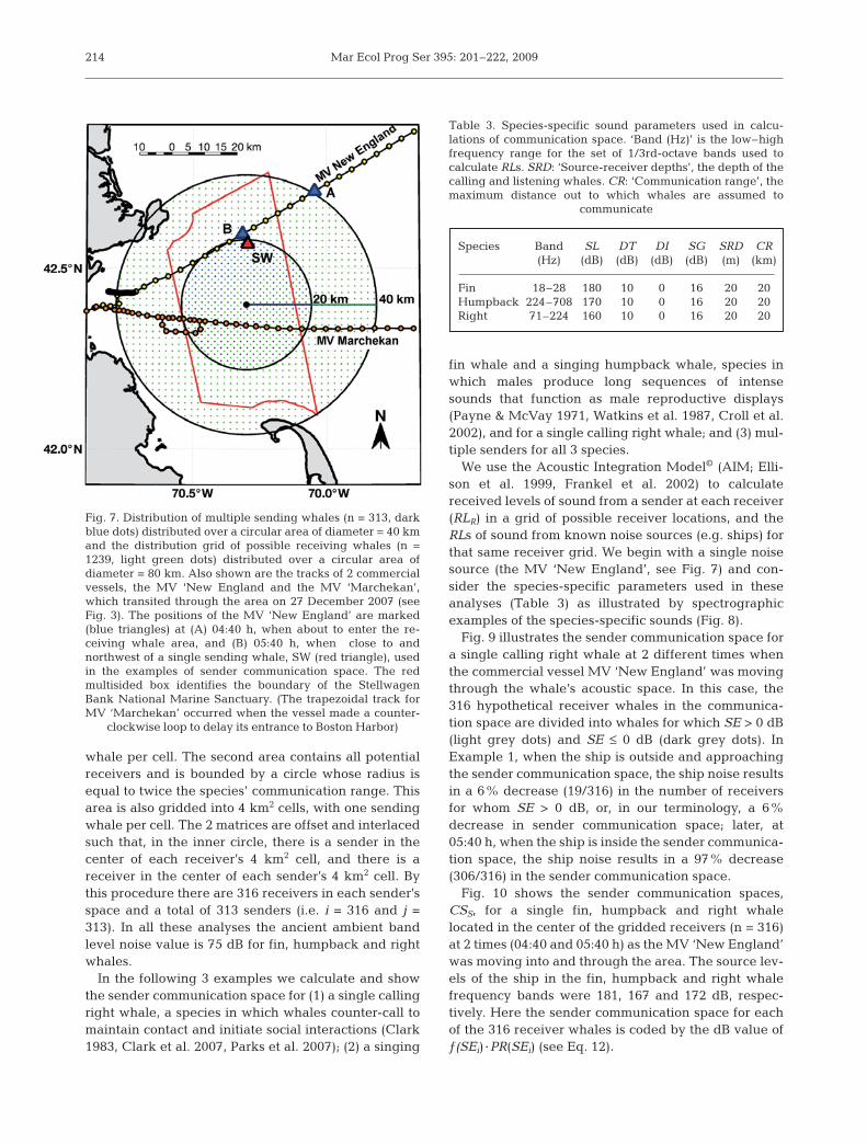
We use the Acoustic Integration Model© (AIM; Elli-son et al. 1999, Frankel et al. 2002) to calculatereceived levels of sound from a sender at each receiver(RLR) in a grid of possible receiver locations, and theRLs of sound from known noise sources (e.g. ships) forthat same receiver grid. We begin with a single noisesource (the MV ‘New England’, see Fig. 7) and con-sider the species-specific parameters used in theseanalyses (Table 3) as illustrated by spectrographicexamples of the species-specific sounds (Fig. 8).

Fig. 9 illustrates the sender communication space fora single calling right whale at 2 different times whenthe commercial vessel MV ‘New England’ was movingthrough the whale’s acoustic space. In this case, the316 hypothetical receiver whales in the communica-tion space are divided into whales for which SE > 0 dB(light grey dots) and SE ≤ 0 dB (dark grey dots). InExample 1, when the ship is outside and approachingthe sender communication space, the ship noise resultsin a 6% decrease (19/316) in the number of receiversfor whom SE > 0 dB, or, in our terminology, a 6%decrease in sender communication space; later, at05:40 h, when the ship is inside the sender communica-tion space, the ship noise results in a 97% decrease(306/316) in the sender communication space.

Fig. 10 shows the sender communication spaces,CSS, for a single fin, humpback and right whalelocated in the center of the gridded receivers (n = 316)at 2 times (04:40 and 05:40 h) as the MV ‘New England’was moving into and through the area. The source lev-els of the ship in the fin, humpback and right whalefrequency bands were 181, 167 and 172 dB, respec-tively. Here the sender communication space for eachof the 316 receiver whales is coded by the dB value ofƒ(SEi) ·PR(SEi) (see Eq. 12).

214

Fig. 7. Distribution of multiple sending whales (n = 313, darkblue dots) distributed over a circular area of diameter = 40 kmand the distribution grid of possible receiving whales (n =1239, light green dots) distributed over a circular area ofdiameter = 80 km. Also shown are the tracks of 2 commercialvessels, the MV ‘New England and the MV ‘Marchekan’,which transited through the area on 27 December 2007 (seeFig. 3). The positions of the MV ‘New England’ are marked(blue triangles) at (A) 04:40 h, when about to enter the re-ceiving whale area, and (B) 05:40 h, when close to andnorthwest of a single sending whale, SW (red triangle), usedin the examples of sender communication space. The redmultisided box identifies the boundary of the StellwagenBank National Marine Sanctuary. (The trapezoidal track forMV ‘Marchekan’ occurred when the vessel made a counter-

clockwise loop to delay its entrance to Boston Harbor)

Species Band SL DT DI SG SRD CR(Hz) (dB) (dB) (dB) (dB) (m) (km)

Fin 18–28 180 10 0 16 20 20Humpback 224–708 170 10 0 16 20 20Right 71–224 160 10 0 16 20 20

Table 3. Species-specific sound parameters used in calcu-lations of communication space. ‘Band (Hz)’ is the low–highfrequency range for the set of 1/3rd-octave bands used tocalculate RLs. SRD: ‘Source-receiver depths’, the depth of thecalling and listening whales. CR: ‘Communication range’, themaximum distance out to which whales are assumed to

communicate

Clark et al.: Acoustic masking in marine ecosystems

Time-varying communication space values of CSS

can be calculated over a portion of the day (27 Dec2007) for each of the 3 species (Fig. 11). These repre-sent the percentage of the communication space avail-able to the sender throughout the 12.3 h period as MV‘New England’ approached, moved through, anddeparted from the communication area.

These 2 examples demonstrate how thecommunication space for a single sendingwhale can vary depending on (1) the proxim-ity of the noise source, (2) the noise level ofthe noise source in the species-specific fre-quency band, (3) the source level of thewhale’s communication sound, and (4) thefrequency band of the whale’s communica-tion sound.

Fig. 12 shows multiple sender communica-tion spaces (CSMS) for 313 hypothetical finwhale singers, humpback whale singers andcalling right whales calculated (see Eq. 15) atthe same 2 times when the MV ‘New England’was moving through the acoustic spaces foreach of the 3 different species. The time-vary-ing values of communication space for each ofthese hypothetical sets of fin whale singers,humpback whale singers and calling rightwhales can be calculated at regular intervals

for the 12 h 20 min time period duringwhich MV ‘New England’ approached,moved through, and departed from thecommunication area (Fig. 13).

The communication spaces for the finand humpback whale singers were onlyslightly changed by the passage of theship and only for the short period of timewhen the ship was very close to thereceiving whales. In contrast, the rightwhale communication space was dra-matically reduced throughout most ofthe time that the ship was passingthrough the area.

One very important outcome from thedevelopment of this algorithm, and illus-trated by these analytical examples, isthat we now have a comparative metricto quantify these differences and varia-tions in communication space for indi-viduals and groups of calling animalsthroughout a habitat and over a selectedperiod of time. Thus, in the exampleabove when considering a single singingfin, singing humpback or calling rightwhale located in the center of the1239 km2 potential CS (Figs. 10 & 11),the sender CS for each species during

the 10 min sample at 05:40 h was 64%, 75%, and 1%,respectively (see Eq. 13). When considering the sets offin, humpback and right whales (n = 313) uniformlydistributed throughout the 1256 km2 area (Figs. 12 &13), the average percentages of sender CS during the10 min sample at 05:40 h were 72%, 84%, and 6%,respectively. For the entire 12 h 20 min period that the

215

Fig. 8. Spectrogram examples showing the repetitive, cadenced features of finwhale song (top); the repeated, syllabic, but subtly variable features of hump-back whale song (middle); and the simple, glissando features of a right whalecontact call (bottom) [1024 pt FFT, 50% overlap, Hanning window]. Note the

different frequency ranges and durations for each of the species

Fig. 9. Spatial distribution of sender CS for a grid of uniformly distributedreceivers (n = 316) based on a calling right whale in the center of the space(SL = 160 dB, DT = –10 dB, SG = 16 dB) and for the noise from the vesselMV ‘New England’ (SL = 172 dB), (A) approaching the sender from thenortheast (see Figs. 3 & 7), and (B) when the ship was 4 km northwest ofthe sender. Light dots: receivers for which SE > 0 dB; dark dots: receivers

for which SE ≤ 0 dB

Mar Ecol Prog Ser 395: 201–222, 2009

MV ‘New England’ was approaching and transitingthrough that area, the average percentage of individ-ual sender CS available was 80% (SD ± 7%) for finwhales, 92% (SD ± 6%) for humpback whales, and23% (SD ± 16%) for right whales.

These examples indicate that calling right whalesare predicted to have been affected to a much greaterextent by masking noise from the MV ‘New England’on 27 Dec 2007 than either singing fin or singinghumpback whales. In fact, the percentage of senderCS available to a uniformly distributed set of callingright whales at this time was estimated to be 3.8 timesless than that for singing humpbacks. During this par-

ticular 12.33 h period, noise from MV ‘New England’resulted in average percentages of communicationmasking for fin, humpback and right whales of 19%(SD ± 0.06), 8% (SD ± 0.05), and 76% (SD ± 0.17),respectively (Fig. 14).

Because the masking algorithm index is generalized(Eq. 10c), we can accumulate additional noise sourcesin the calculation of M. Thus, for example, when mask-ing noise from a second ship (MV ‘Marchekan’, 14:50to 20:50 h; see Fig. 7) is added to the noise from MV‘New England’, the accumulated noise during the 21 hperiod (01:10 h to 22:10 h) increases the average per-centages of communication masking for fin, humpbackand right whales to 33% (SD ± 0.14), 11% (SD ± 0.06),and 84% (SD ± 0.16), respectively (Fig. 15).

DISCUSSION

Ocean ambient noise and noise sources mask thecommunication sounds of free-ranging marine mam-mals. A mechanism is described for quantitativelyassessing communication masking for one or manysending animals as a result of one or more noisesources13. Here the term communication masking is amodification of the term as originally developed forhuman speech. In the clinical sense, communicationmasking is the amount (or process) by which thethreshold of audibility of one sound is raised by thepresence of another (masking) sound (Tanner 1958,Moore 1982). We redefine the term communicationmasking for the practical situation in which free-

216

Fig. 11. Time-varying percentages of CSS (Eq. 13), as a functionof ship noise, for a single fin whale singer, humpback whalesinger and calling right whale during the passage of MV ‘NewEngland’ through the SBNMS on 27 December 2007. Sampleswere taken every 10 min from 01:10 to 13:30 h. The 2 arrowscorrespond to the 2 sample times (04:40 and 05:40 h) shown

in Fig. 10

Fig. 10. Spatial distributions of sender CS for a single finwhale singer (A, B), humpback whale singer (C,D) and call-ing right whale (E, F) as a function of noise from an approach-ing ship, the MV ‘New England’. The sending whale islocated in the center of a 1256 km2 CS of 316 receivingwhales. Left hand panels are at 04:40 h when the ship wasnortheast of the sender. Right hand panels are at 05:40 hwhen the ship was ~4 km northwest of the sender. The scalebar indicates the recognition-weighted value of SE in dB at

the receiver locations (Eq. 12)

13Values of CS and M for receiving individuals or populationsare similarly derived but are not the same as for sending animals.

Clark et al.: Acoustic masking in marine ecosystems

ranging marine mammals are communicating underthe acoustic conditions present within their existinghabitats. Under this real-world context, communica-tion masking is measured as a loss of communicationspace as a result of other sound(s), either natural oranthropogenic, relative to that space under quietancient ambient conditions; where we use the 5th per-centile noise level as that reference for quiet noise.

We have merged the well established and empiri-cally-based knowledge of ocean acoustic propagationmodeling and the sonar equation, and informed thesewith empirical biological parameters and biologicalconsiderations relative to space, frequency and time.By tuning these parameters to the actual bioacousticcharacteristics of communication sounds for differentspecies we calculate measures that quantify the spatio-spectral-temporal variability of a species’ communica-

tion space in real-world conditions involving humansound sources. The result is a metric by which one cansystematically measure and compare changes in com-munication space as a result of anthropogenicsound(s); in the case here, the noise from a commercialship moving through a marine sanctuary in which atleast 3 species have seasonal residence.

We demonstrate that it is possible to assign objective,quantitative values to the communication masking offree-ranging marine mammals operating in the pres-ence of real-world anthropogenic noise sources, and toprovide insight into the potential effects of communi-cation masking by ship noise on fin, humpback andright whales in an important coastal habitat. This pro-cess can be expanded and applied to other species, inother biological contexts, in other habitats, and on dif-ferent spatial and temporal scales.

Communication masking by ship noise is much moresevere for calling right whales than it is for singing finor humpback whales in the examples considered here(see Figs. 13 to 15). In these analyses a major reason forthis difference is source level: right whale calls are notas loud as fin or humpback songs. Combined withdifferences in source level are the differences in thespecies-specific, noise band levels from the ship; 181,167, and 172 dB for fin, humpback and right whales,respectively (NSL re 1µPA @1 m) and the differenttransmission losses for the noise in those different fre-quency bands. What is not considered here is sourcelevel variability; right whales certainly do not alwayscall at 160 dB or fin whales at 180 dB; or the actual vari-ability in a species’ recognition threshold, which wehave simplified by assuming that all 3 species have a

217

Fig. 13. Time-varying percentages of CSMS (Eq. 15) availablefor a uniformly distributed number of fin whale singers,humpback whale singers and calling right whales (n = 313,see Fig. 12) on 27 December 2007. Samples taken every

10 min from 01:10 to 13:30 h

Fig. 12. Spatial distributions of CS for a uniformly distributednumber of fin whale singers, humpback whale singers andcalling right whales (n = 313) and for noise from an approach-ing ship, the MV ‘New England’. Left-hand panels are at04:40 h when the ship was ∼40 km to the northeast of the clos-est sender, and right-hand panels are at 05:40 h when the shipwas ~4 km to the northwest of the closest sender (see Figs. 3& 7). (A, B) fin whale; (C, D) humpback whale; (E, F) rightwhale. Scale bar indicates the CSMS value (see Eq. 15)

Mar Ecol Prog Ser 395: 201–222, 2009

signal processing gain of 16 dB; or the areas overwhich these animals actually communicate, which wehave simplified by assuming that all 3 species onlycommunicate out to a range of 20 km.

These basic considerations emphasize the need toknow more about the characteristics of communicationsignals, the conditions under which animals actuallyproduce these signals, and how they might vary theircommunications under different contexts. Almostevery term and parameter is a function of multiplevariables, and the variance in each of these variablesimposes different amounts of uncertainty on the out-come of any estimate of communication masking.However, these uncertainties are bounded and theirsimplification allows one to calculate estimates thatare at least good first order approximations. There-

fore, these estimates are useful for assessing the poten-tial for communication masking on different whalespecies.

Knowing the biological and abiotic parameters (e.g.frequency band, integration time, communicationrange, call source level of animal’s sound, depth ofcalling and receiving animals, anthropogenic noisesource characteristics and movements, propagationloss features) one can envision how noise might maskthe communication space of a roving herd of pilotwhales whistling in the 7–12k Hz band at 175 dB (SL re1µPa @1m). Given the much higher transmission lossand lower source levels of ships at these frequencies aswell as the expected smaller communication space forpilot whales under normally quiet conditions, onemight predict that the spatio-spectral-temporal foot-print of communication masking from the ship noise onpilot whales would be much smaller than that for thebaleen whales. The benefit from the algorithm pre-sented in this paper is that it provides an analyticalprocess by which to quantify what is meant by ‘muchsmaller’.

Our considerations can be extended to non-continu-ous sources of noise (e.g. the low-frequency energyfrom seismic airgun arrays or construction activities)and acoustic contexts other than communication (e.g.echolocation or predator avoidance). A conclusion thatis common to all, and independent of species or contextis that the greatest uncertainties in our abilities to esti-mate the impacts of communication masking comefrom our ignorance of the spatial and temporal scalesover which animals engage in their bioacoustic activi-ties. Fairly little is known about the ranges over whichthe large whales actually communicate, althoughbased on signal and receiver characteristics some esti-mates of communication distances are possible. How-ever, without better knowledge certain assumptionsabout communication range are required and theresultant uncertainties in estimates of communicationmasking are dependent on those assumptions.

An important outcome (exemplified in Fig. 15) is thatthis communication masking algorithm can be used toevaluate the contributions to masking from individualsound sources and the cumulative effect of multiplesources on one or many individuals. Cumulative im-pact has been a long-standing, seemingly intractableissue in the debate over noise effects on marine mam-mals. Here we have presented a standardized metric toquantitatively estimate how much each sound sourcecontributes to the communication masking index.Stated from an ecological perspective, we now have ameasure for estimating the cost to communication,measured and expressed over ecologically meaningfulspatial and temporal scales, for an individual or a pop-ulation as a result of a particular sound source. Thus,

218

Fig. 14. M for a uniformly distributed number of fin whalesingers, humpback whale singers and calling right whales(see Fig. 12 & 13) on 27 December 2007 as a result of noisefrom the MV ‘New England’. Samples were taken every

10 min from 01:10 to 13:30 h

Fig. 15. Cumulative M for a uniformly distributed number offin whale singers, humpback whale singers and calling rightwhales (see Fig. 14) on 27 December 2007 as a result of noisefrom 2 ships, the MV ‘New England’ and the MV ‘Marche-kan’. Samples were taken every 10 min from 01:10 to 22:10 h

Clark et al.: Acoustic masking in marine ecosystems

using right whales as an example, we have shown thatfor at least 13.2 h of one day in the SBNMS the averagecommunication masking index was 0.84, or the cost tocommunication from 2 commercial ships was an 84%reduction of communication space, i.e. on average only16% of a whale’s expected communication space wasavailable. Based on data in Hatch et al. (2008) indicat-ing an average of 6 commercial vessels per day over a2 mo period, we can assume that this magnitude ofimpact on potential right whale communication spaceoccurs for much of the time that whales are in thathabitat. This raises specific questions as to the cost toan individual right whale from this chronic noise con-dition and how the loss of communication opportuni-ties might lead to decreased fecundity and rates of sur-vival. At present we can only speculate because we donot know enough of the details about when and howthe whales use their calls to communicate relative tothe behavioral and ecological contexts, and howreductions in these capabilities translate into biologicalcost. We do know that these whales counter-call anduse these episodes of calling to find each other and toaggregate, so one immediate cost is the loss of oppor-tunities to form social groups. Right whales formaggregations during mating and during feeding, soone likely cost is the loss of mating and feeding op-portunities. However, we do not yet know the realcost to an individual or a population from these lostopportunities.

The application and extension of the communica-tion masking metric to quantify biological cost withinan ecological framework offers a critical missing linkto the major current dilemma of assessing noiseimpacts in the marine environment. As representedby the Potential Consequences of Acoustic Distur-bance (PCAD) model (NRC 2005), there is a cascadeof transitions between 5 core components in themodel starting with physical acoustics and endingwith population level effects. Each transition betweenmodel components shows the output(s) from one com-ponent as the input(s) into the next and then assumesthat a response in the next component is a function ofthe input(s). The model provides no specific enlight-enment as to how the transitions between componentsoccur, or what the transfer functions are. In fact, thetransitions as presently stated confound different lev-els of analysis because the model does not specificallydeal with the fact that the input-output variablesbetween different components are often conceptual orhave fundamentally different units. Thus, the PCADmodel in its present form provides little explicit direc-tion towards a practical solution; we offer a steptoward a solution by formalizing the functional con-nections between spatio-spectral-temporal variabilityin a free-ranging animal’s ambient noise environment

and the resultant loss of its opportunities to communi-cate. The task now is to better understand and con-strain the uncertainties in the algorithm’s variables,and to inform some of the simplifying assumptions(and test predicted ranges) with more empirical data.That will, of course, require addressing communica-tion ranges within the proper ecological contexts and,more generally, the spaces over which differentacoustic behaviors occur and change as a function ofnoise and other events.

We have adapted the term communication maskingto the marine world of today, in which animals are con-fronted with a dynamic multitude of broadbandsources added to a less dynamic, but steadily risingbaseline of ambient noise that is considerably different(from the perspective of the animals) and more difficultto communicate in than the ambient acoustic ecologyin which they evolved. The acoustic ecology of thismodern habitat has changed significantly within thelifetime of an individual, thereby short-circuiting thenormal operations of selection and adaptation. If ani-mals are not pre-adapted or well adapted to compen-sate for changes in their ambient noise environment,they are left with few, if any, options by which to suc-cessfully communicate in anthropogenically modifiedacoustic habitats. There is some evidence that whalescan, but sometimes do not, compensate for suchchanges in their ambient noise environment. Forexample, killer whales increase the amplitudes of theircalls with increasing noise in the 1–40 kHz frequencyband (Holt et al. 2009), and blue whales increase theirrate of social calling in the presence of noise from aseismic exploration sparker (Di Iorio & Clark 2009).North Atlantic right whales have shifted the funda-mental frequency of their contact calls by about anoctave over a period of several decades, possibly as aresult of long-term increases in ambient noise, but theyreduce calling rate in response to increases in localambient noise conditions (Parks et al. 2007).

Payne & Webb (1971) were the first to raise the con-cern that noise from modern commercial shippingmight reduce long-range communication for blue andfin whale singers. That hypothesis was ignored for aquarter of a century, during which ambient oceannoise levels continued to rise. By the century’s turn thatconcern could no longer be ignored (e.g. NRC 2000,2003). Numerous workshops were held to formally dis-cuss and debate the problem (e.g. Southall 2005,Southall & Scholik-Schlomer 2009), and in some casesthose discussions have led to agreements on actionsthat could lead to reductions in ocean noise levels(Wright 2008).

As demonstrated here, the acoustic communicationspace for at least one species of large baleen whale, thehighly endangered North Atlantic right whale, is seri-

219

Mar Ecol Prog Ser 395: 201–222, 2009

ously compromised by noise from commercial shippingtraffic. It remains to be determined over what spatial-spectral-temporal scales this conclusion is applicableto other species and other habitats.

As the planet’s present dominant species, humanshave choices to make. In the case of the ocean’sacoustic ecological habitat, the choices we are makingnow have profound implications for the future ofmarine mammals. It is our opinion that the right choicecannot wait another 3 decades.

Acknowledgements. C.W.C. thanks Roger Payne for hisnumerous shared insights and our conversations on the topicof large-scale implications of anthropogenic noise on largewhale, low-frequency acoustic communication; and GeorgeC. Gagnon (Ret. LCR US Navy) for sharing his insights andfirst-hand knowledge of low-frequency ocean acoustics, andfor his unwavering quest for learning more about sound in theocean. The authors are grateful for publications by or conver-sations with numerous colleagues, including Moira Brown,Peter Corkeron, Kurt Fristrup, David Kastak, Scott Kraus,Stormy Mayo, Susan Parks, Colleen Reichmuth, W. JohnRichardson, Rosalind Rolland, and Ronald Schusterman. Weacknowledge scientists and staff at Stellwagen Bank NationalMarine Sanctuary and the Northeast Fisheries Science Cen-ter, and in particular Michael Thompson and Denise Risch.C.W.C. acknowledges the scientists, engineers and staff inthe Bioacoustics Research Program at Cornell; particularlyTom Calupca, Robert MacCurdy, and Ildar Urazghildiiev fortheir assistance with data collection and analysis. DavidJaniger of the Natural History Museum of Los AngelesCounty assisted with the literature search. We thank W. JohnRichardson and 2 anonymous reviewers for constructive criti-cism of an earlier version of the manuscript. Funding for thedata presented herein was provided under NOPP-ONR Grant#N00014-07-1-1029 and contracts with Commonwealth ofMassachusetts Division of Marine Fisheries, ExcelerateEnergy and Suez Energy LLC (C.W.C.).

LITERATURE CITED

Andrew RK, Howe BM, Mercer JA, Dzieciuch MA (2002)Ocean ambient sound: Comparing the 1960’s with the1990s for a receiver off the California coast. ARLO 3:65–70

Arons B (1992) A review of the cocktail party effect. J AmVoice I/O Soc 12:35–50

Au WWL (1993) The sonar of dolphins. Springer-Verlag, NewYork

Beranek LL, Ver IL (1992) Noise and vibration control engi-neering. Wiley, New York

Bregman AS (1990) Auditory scene analysis: the perceptualorganization of sound. MIT Press, Cambridge, MA

Brenowitz EA (1982) The active space of red-winged black-bird song. J Comp Physiol [A] 147:511–522

Broadbent DE (1958) Perception and communication. Perga-mon, New York

Brown CH (1989) The active space of blue monkey and grey-cheeked mangabey vocalizations. Anim Behav 37:1023–1034

Brungart DS (2004) Informational and energetic maskingeffects in multitalker speech perception. In: Divenji P (ed)Speech separation by humans and machines. Kluwer Aca-demic Press, Boston, MA, p 261–267

Cherry EC, Taylor WK (1954) Some further experiments uponthe recognition of speech, with one and with two ears.J Acoust Soc Am 26:554–559

Clark CW (1983) Acoustic communication and behavior of thesouthern right whale (Eubalaena australis). In: Payne R(ed) Communication and behavior of whales. WestviewPress, Boulder, CO, p 163–198

Clark CW (1989) Call tracks of bowhead whales based on callcharacteristics as an independent means of determiningtracking parameters. Rep Int Whaling Comm 39:111–112

Clark CW (1990) Acoustic behavior of mysticete whales. In:Thomas J, Kastelein R (eds) Sensory abilities of cetaceans.Plenum Press, New York, p 580–583

Clark CW, Ellison WT (2004) Potential use of low-frequencysounds by baleen whales for probing the environment:evidence from models and empirical measurements. In:Thomas JA, Moss CF, Vater M (eds) Advances in the studyof echolocation in bats and dolphins. University ofChicago Press, Chicago, IL, p 564–589

Clark CW, Gagnon GC (2002) Insights from IUSS detections,locations and tracking from 1992 to 1996. J UnderwaterAcoust 52:609–640

Clark CW, Borsani JF, Notarbartolo di Sciara G (2002) Vocalactivity of fin whales, Balaenoptera physalus, in the Lig-urian Sea. Mar Mamm Sci 18:286–295

Clark CW, Gillespie D, Nowacek DP, Parks SE (2007) Listen-ing to their world: Acoustics for monitoring and protectingright whales in an urbanized ocean. In: Kraus S, Rolland R(eds) The urban whale. Harvard University Press, Cam-bridge, MA, p 333–357

Cox TM, Ragen TJ, Read AJ, Vos E and others (2006) Under-standing the impacts of anthropogenic sound on beakedwhales. J Cetacean Res Manag 7:177–187

Croll DA, Clark CW, Acevedo A, Tershy B, Floress S,Gedamke J, Urban J (2002) Only male fin whales singloud songs. Nature 417:809

Di Iorio L, Clark CW (2009) Exposure to seismic survey altersblue whale acoustic communication. Biol Lett doi:10.1098/rsbl.2009.0651

Durlach NI, Colburn HS (1978) Binaural phenomena. In:Carterette EC, Friedman MP (eds) Handbook of percep-tion, Vol IV. Academic Press, New York, p 365–455

Ellison WT, Weixel K, Clark CW (1999) An acoustic integra-tion model (AIM) for assessing the impact of underwaternoise on marine wildlife. J Acoust Soc Am 106:2250

Erbe C, Farmer DM (2000) A software model to estimatezones of impact on marine mammals around anthro-pogenic noise. J Acoust Soc Am 108:1327–1331

Evans GW (2001) Environmental stress and health. In: BaumA, Revenson T, Singer JE (eds) Handbook of health psy-chology. Erlbaum Press, Mahway, NJ

Evans GW (2003) A multimethodological analysis of cumu-lative risk and allostatic load among rural children. DevPsychol 39:924–933

Fay RR (1988) Hearing in vertebrates: a psychophysics data-book. Worcester Heffernan Press, Worcester, MA

Fay RR (1992) Structure and function of sound discriminationamong vertebrates. In: Webster DB, Fay RR, Popper AN(eds) The evolutionary biology of hearing. Springer-Verlag, New York, p 229–263

Finneran JJ, Oliver CW, Schaefer KM, Ridgway SH (2000)Source levels and estimated yellowfin tuna (Thunnusalbacares) detection ranges for dolphin jaw pops,breaches, and tail slaps. J Acoust Soc Am 107:649–656

Fletcher H (1940) Auditory patterns. Rev Mod Phys 12:47–65Frankel AS, Ellison WT, Buchanan J (2002) Application of the

Acoustic Integration Model (AIM) to predict and minimize

220

Clark et al.: Acoustic masking in marine ecosystems

environmental impacts. IEEE Oceans 2002:1438–1443Handel S (1989) Listening: an introduction to the perception

of auditory events. MIT Press, Cambridge, MAHarrison C, Harrison J (1995) A simple relationship between

frequency and range averages for broadband sonar. JAcoust Soc Am 97:1314–1317

Hatch L, Clark C, Merrick R, Van Parijs S and others (2008)Characterizing the relative contributions of large vesselsto total ocean noise fields: A case study using the Gerry E.Studds Stellwagen Bank National Marine Sanctuary. Env-iron Manage 42:735–752

Holt MM, Schusterman RJ (2007) Spatial release from mask-ing of aerial tones in pinnipeds. J Acoust Soc Am 121:1219–1225

Holt MM, Noren DP, Veirs V, Emmons CK, Veirs S (2009)Killer whales (Orcinus orca) increase their call amplitudein response to vessel noise. J Acoust Soc Am 125:EL27–EL32

Ihlefeld A, Shinn-Cunningham B (2008) Spatial release fromenergetic and informational masking in a selective speechidentification task. J Acoust Soc Am 123:4369–4379

Janik VM (2000) Source levels and the estimated active spaceof bottlenose dolphin (Tursiops truncatus) whistles in theMoray Firth, Scotland. J Comp Physiol [A] 186:673–680

Kastelein RA, de Hann D, Verboom WC (2007) The influenceof signal parameters on the sound source localization abil-ity of a harbor porpoise (Phocoena phocoena). J AcoustSoc Am 122:1238–1248

Kryter KD (1994) The handbook of hearing and the effects ofnoise: physiology and public health. McGraw-Hill, NewYork

McDonald MA, Hildebrand JA, Wiggins SM (2006) Increasesin deep ocean ambient noise in the Northeast Pacific westof San Nicolas Island, California. J Acoust Soc Am 120:711–718

Miller JL (1997) Speech perception. In: Crocker MJ (ed) Ency-clopedia of acoustics, Vol IV. John Wiley & Sons, NewYork, p 1579–1588

Moore BCJ (1982) An introduction to the psychology of hear-ing. Academic Press, London

Moore SE, Stafford Kathleen M, Mellinger DK, HildebrandJA (2006) Listening for large whales in the offshore watersof Alaska. BioScience 56:49–55

NRC (National Research Council) (2000) Marine mammalsand low-frequency sound: progress since 1994. NationalAcademies Press, Washington, DC

NRC (National Research Council) (2003) Ocean noise andmarine mammals. National Academies Press, Washington,DC

NRC (National Research Council) (2005) Marine mammalpopulations and ocean noise: Determining when noisecauses biologically significant effects. National Acade-mies Press, Washington, DC

Niemiec AJ, Yost WA, Shofner WP (1992) Behavioral mea-sures of frequency selectivity in the chinchilla. J AcoustSoc Am 92:2636–2649

Nilsson M, Sigfrid DS, Sullivan JA (1994) Development of thehearing in noise test for the measurement of speech recep-tion thresholds in quiet and in noise. J Acoust Soc Am95:1085–1099

Nowacek DP, Thorne LH, Johnston DW, Tyack PL (2007)Responses of cetaceans to anthropogenic noise. MammalRev 37:81–115

Parks SE, Clark CW, Tyack PL (2007) Short- and long-termchanges in right whale calling behavior: The potentialeffects of noise on acoustic communication. J Acoust SocAm 122:3725–3731

Payne RS, McVay S (1971) Songs of humpback whales.Science 173:585–597

Payne R, Webb D (1971) Orientation by means of long rangeacoustic signaling in baleen whales. Ann NY Acad Sci188:110–142

Pearsons KS, Bennett RL, Fidell S (1977) Speech levels in var-ious noise environments. US Environmental ProtectionAgency, Washington, DC

Peters S, Stubley P, Valin J (1999) On the limits of speech recog-nition in noise. In: Spanias A, Cochran D (eds) IEEE Interna-tional Conference on Acoustics, Speech and Signal Process-ing. IEEE Computer Society, Washington, DC, p 365–368

Porter M, Reiss EL (1985) A numerical method for bottominteracting ocean acoustic normal modes. J Acoust SocAm 77:1760–1767

Premus V, Spiesberger JL (1997) Can acoustic multipathexplain finback (B. physalus) 20-Hz doublets in shallowwater? J Acoust Soc Am 101:1127–1138

Reynolds JE III, Rommel SA (1999) Biology of marine mam-mals. Smithsonian Books, Washington, DC

Richardson WJ, Greene CR, Malme CI, Thomson DH (1995)Marine mammals and noise. Academic Press, San Diego,CA

Scharf B (1970) Critical bands. In: Tobias JV (ed) Foundationsof modern auditory theory, Vol. 1. Academic Press, NewYork, p 159–202

Schultz TJ (1978) Synthesis of social surveys on noise annoy-ance. J Acoust Soc Am 64:377–405

Schusterman RJ (1981) Behavioral capabilities of seals andsea lions: a review of their hearing, visual, learning anddiving skills. Psychol Rec 31:125–143

Southall BL (2005) ‘Shipping noise and marine mammals: aforum for science, technology, and management.’ Finalreport, National Oceanic and Atmospheric Administra-tion, Washington, DC

Southall BL, Scholik-Schlomer A (2009) Potential applicationof vessel-quieting technology on large commercial ves-sels. Final Report of the National Oceanic and Atmos-pheric Administration (NOAA) International Conference.NOAA Fisheries, Silver Spring, MD

Southall BL, Schusterman RJ, Kastak D (2003) Acoustic com-munication ranges for northern elephant seals (Miroungaangustirostris). Aquat Mamm 29:202–213

Southall BL, Bowles AE, Ellison WT, Finneran JJ and others(2007) Marine mammal noise exposure criteria: Initial sci-entific recommendations. Aquat Mamm 33:411–414

Stafford KM, Mellinger DK, Moore SE, Fox CG (2007) Sea-sonal variability and detection range modeling of baleenwhale calls in the Gulf of Alaska, 1999–2002. J Acoust SocAm 122:3378–3390

Tafalla R, Evans G (1997) Noise, physiology, and humanperformance: the potential role of effort. J Occup HealthPsychol 2:148–155

Tanner WP (1958) What is masking? J Acoust Soc Am 30:919–921

Turnbull SD (1994) Changes in masked thresholds of a harborseal (Phoca vitulina) associated with angular separation ofsignal and noise sources. Can J Zool 72:1863–1866

Tyack PL (1998) Acoustic communication under the sea. In:Hopp SL, Owren MJ, Evans CS (eds) Animal acousticcommunication: Sound analysis and research methods.Springer-Verlag, New York, p 163–220

Tyack PL (2008) Implications for marine mammals of large-scale changes in the marine acoustic environment.J Mammal 89:549–558

Urick RJ (1983) Principles of underwater sound. McGraw-Hill, New York

221

Mar Ecol Prog Ser 395: 201–222, 2009

Wartzok D, Ketten DR (1999) Marine mammal sensory sys-tems. In: Reynolds JE III, Rommel SA (eds) Biology ofmarine mammals. Smithsonian Institute Press, Washing-ton, DC, p 117–175

Watkins WA (1981) Activities and underwater sounds of finwhales. Sci Rep Whales Res Inst 33:83–117

Watkins WA, Schevill WE (1979) Aerial observation of feed-ing behavior in four baleen whales: Eubalaena glacialis,Balaenoptera borealis, Megaptera novaeangliae, and Bal-aenoptera physalus. J Mammal 60:155–163

Watkins WA, Tyack P, Moore KE (1987) The 20-Hz signals offinback whales (Balaenoptera physalus). J Acoust Soc Am82:1901–1912

Watkins WA, Daher MA, George JE, Rodriguez D (2004)Twelve years of tracking 52-Hz whale calls from a uniquesource in the North Pacific. Deep Sea Res I 51:1889–1901

Watson CS (1987) Uncertainty, informational masking and thecapacity of immediate auditory memory. In: Yost WA,Watson CS (eds) Auditory processing of complex sounds.Erlbaum, Hillsdale, NJ, p 267–277

Wegel RL, Lane CE (1924) The auditory masking of one puretone by another and its probable relation to the dynamicsof the inner ear. Phys Rev 23:266–285

Wright AJ (ed) (2008) International Workshop on ShippingNoise and Marine Mammals, Hamburg, Germany, 21–24April 2008. Okeanos—Foundation for the Sea, Darmstadt.Available from www.sound-in-the-sea.org/download/ship2008_en.pdf

Yost WA (2000) Fundamentals of hearing. Academic Press,San Diego, CA

Yost WA, Popper AN, Fay RR (2008) Auditory perception ofsound sources. Springer, New York

222

Submitted: December 26, 2008; Accepted: November 9, 2009 Proofs received from author(s): November 29, 2009