Embed Size (px)
Citation preview
ISCAS: June 1, 1998 1
A Baseband Pulse Shaping Filter for
Gaussian Minimum Shift Keying
N. Krishnapura1, S. Pavan2,
C. Mathiazhagan3, B. Ramamurthi3
1 Dept. of EE, Columbia University, New York, USA.2 Texas Instruments, Edison, New Jersey, USA.
3 Dept. of EE, Indian Institute of Technology, Chennai, India.

2
Motivation
• Rectangular bit stream has a large amount of energyat high frequencies.
• Pulse shaping limits the out of band radiation incommunication systems.
• Digital pulse shaping - harder with high bit rates.
• Analog pulse shaping → lower power and area?
3
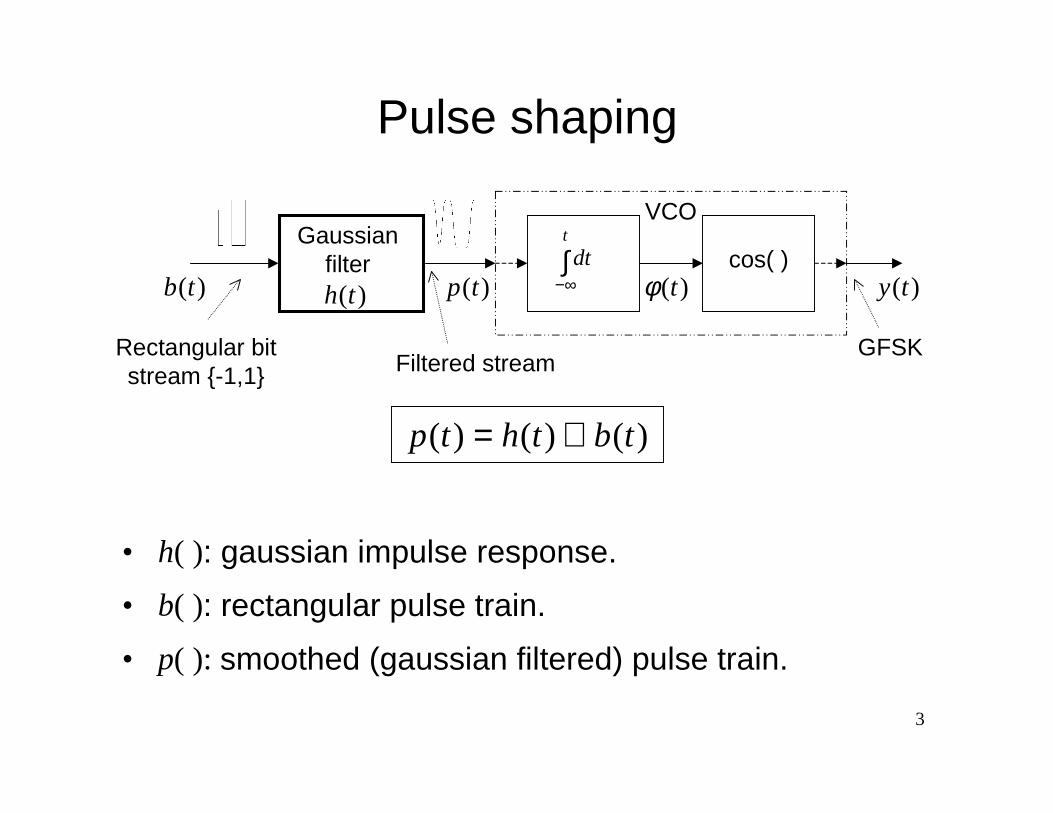
Pulse shaping
• h( ): gaussian impulse response.
• b( ): rectangular pulse train.
• p( ): smoothed (gaussian filtered) pulse train.
)(tp
Gaussianfilter cos( )
Rectangular bitstream {-1,1} Filtered stream
VCO
GFSK
)(tφ )(ty)(th)(tb∫∞−
t
dt
)()()( tbthtp ⊗=
4
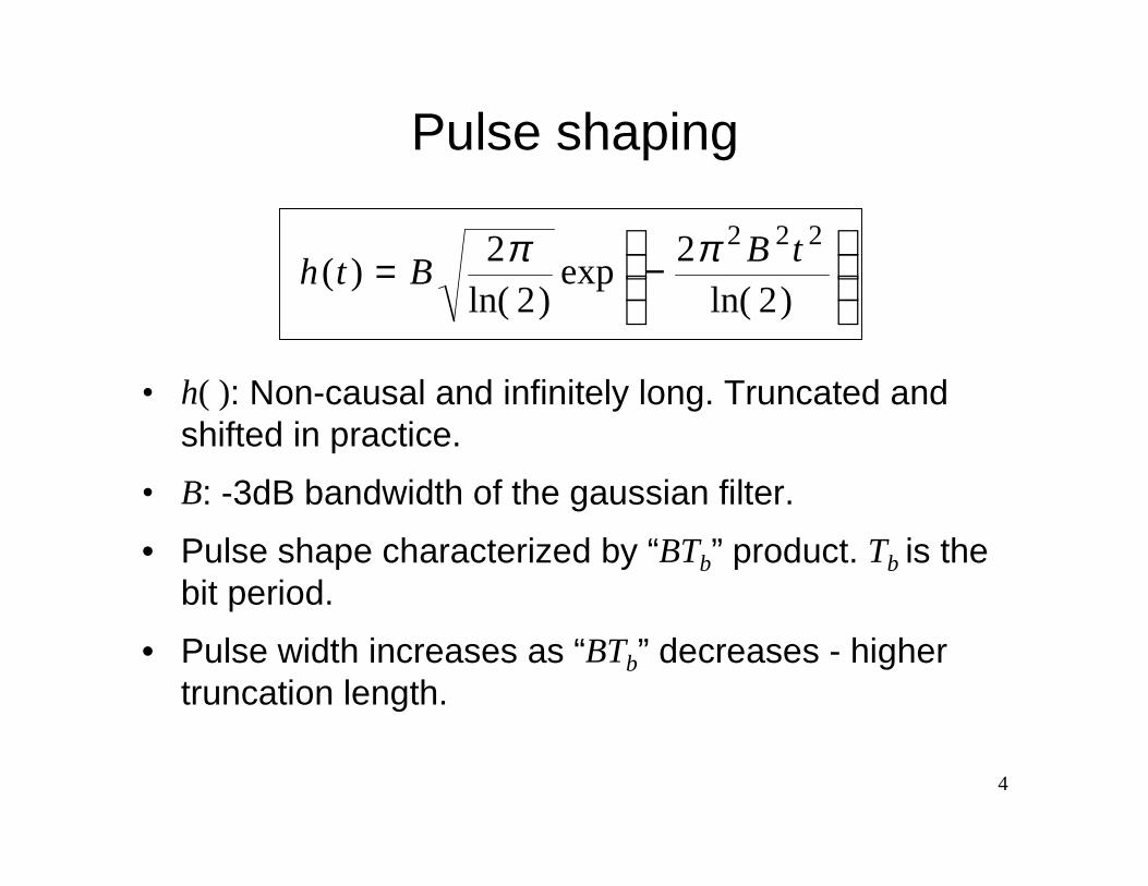
Pulse shaping
−=
)2ln(2
exp)2ln(
2)(
222 tBBth
ππ
• h( ): Non-causal and infinitely long. Truncated andshifted in practice.
• B: -3dB bandwidth of the gaussian filter.
• Pulse shape characterized by “BTb” product. Tb is thebit period.
• Pulse width increases as “BTb” decreases - highertruncation length.
5
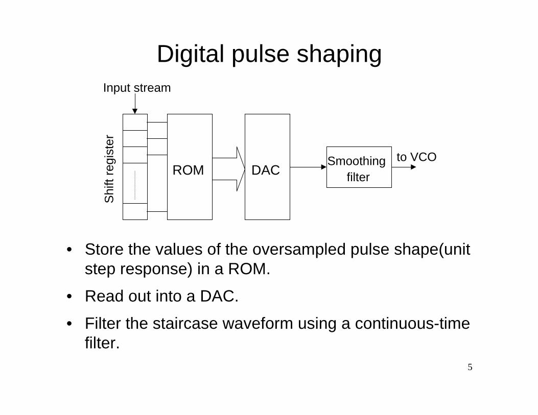
Digital pulse shaping
• Store the values of the oversampled pulse shape(unitstep response) in a ROM.
• Read out into a DAC.
• Filter the staircase waveform using a continuous-timefilter.
Shi
ft re
gist
er
ROM DACSmoothing
filter
Input stream
to VCO
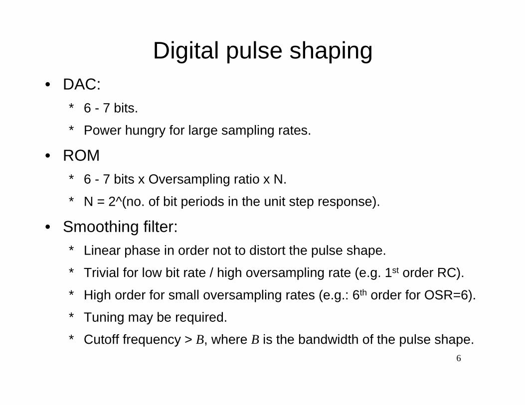
6
Digital pulse shaping• DAC:
* 6 - 7 bits.
* Power hungry for large sampling rates.
• ROM* 6 - 7 bits x Oversampling ratio x N.
* N = 2^(no. of bit periods in the unit step response).
• Smoothing filter:* Linear phase in order not to distort the pulse shape.
* Trivial for low bit rate / high oversampling rate (e.g. 1st order RC).
* High order for small oversampling rates (e.g.: 6th order for OSR=6).
* Tuning may be required.
* Cutoff frequency > B, where B is the bandwidth of the pulse shape.
7
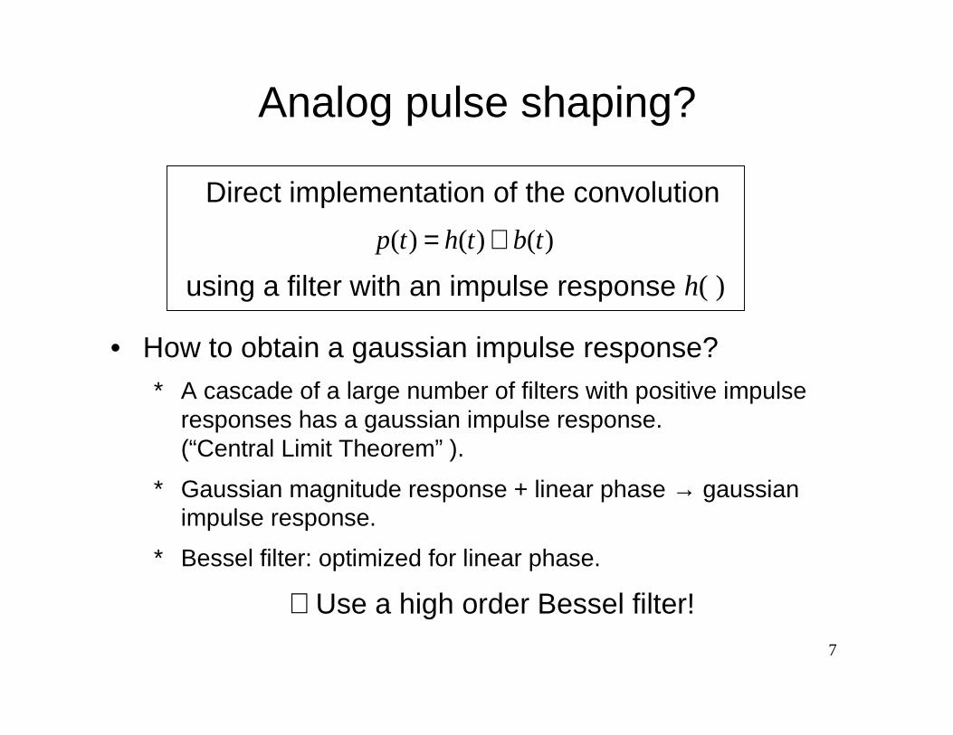
Analog pulse shaping?
• How to obtain a gaussian impulse response?* A cascade of a large number of filters with positive impulse
responses has a gaussian impulse response.(“Central Limit Theorem” ).
* Gaussian magnitude response + linear phase → gaussianimpulse response.
* Bessel filter: optimized for linear phase.
∴Use a high order Bessel filter!
Direct implementation of the convolution
)()()( tbthtp ⊗=
using a filter with an impulse response h( )
8
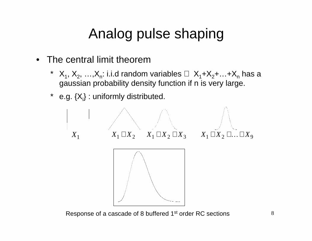
Analog pulse shaping
• The central limit theorem
* X1, X2, …,Xn: i.i.d random variables ⇒ X1+X2+…+Xn has agaussian probability density function if n is very large.
* e.g. {Xi} : uniformly distributed.
1X 21 XX + 321 XXX ++ 921 XXX +++ �
Response of a cascade of 8 buffered 1st order RC sections
9
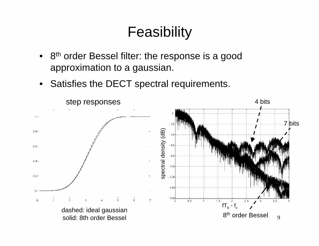
Feasibility
• 8th order Bessel filter: the response is a goodapproximation to a gaussian.
• Satisfies the DECT spectral requirements.
step responses
dashed: ideal gaussiansolid: 8th order Bessel
4 bits
7 bits
8th order Bessel
spe
ctra
l den
sity
(dB
)
fTb - fc
10
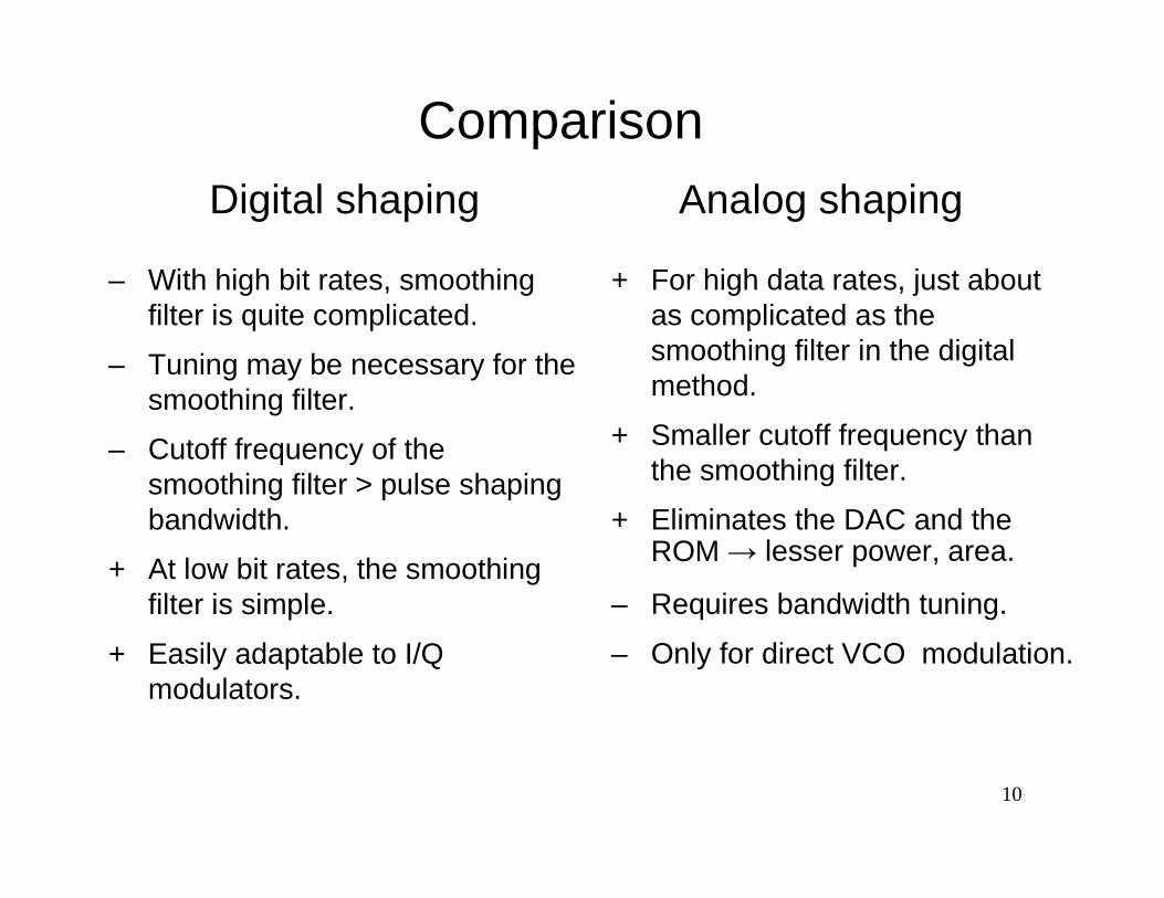
Comparison
– With high bit rates, smoothingfilter is quite complicated.
– Tuning may be necessary for thesmoothing filter.
– Cutoff frequency of thesmoothing filter > pulse shapingbandwidth.
+ At low bit rates, the smoothingfilter is simple.
+ Easily adaptable to I/Qmodulators.
+ For high data rates, just aboutas complicated as thesmoothing filter in the digitalmethod.
+ Smaller cutoff frequency thanthe smoothing filter.
+ Eliminates the DAC and theROM � lesser power, area.
– Requires bandwidth tuning.
– Only for direct VCO modulation.
Digital shaping Analog shaping
11
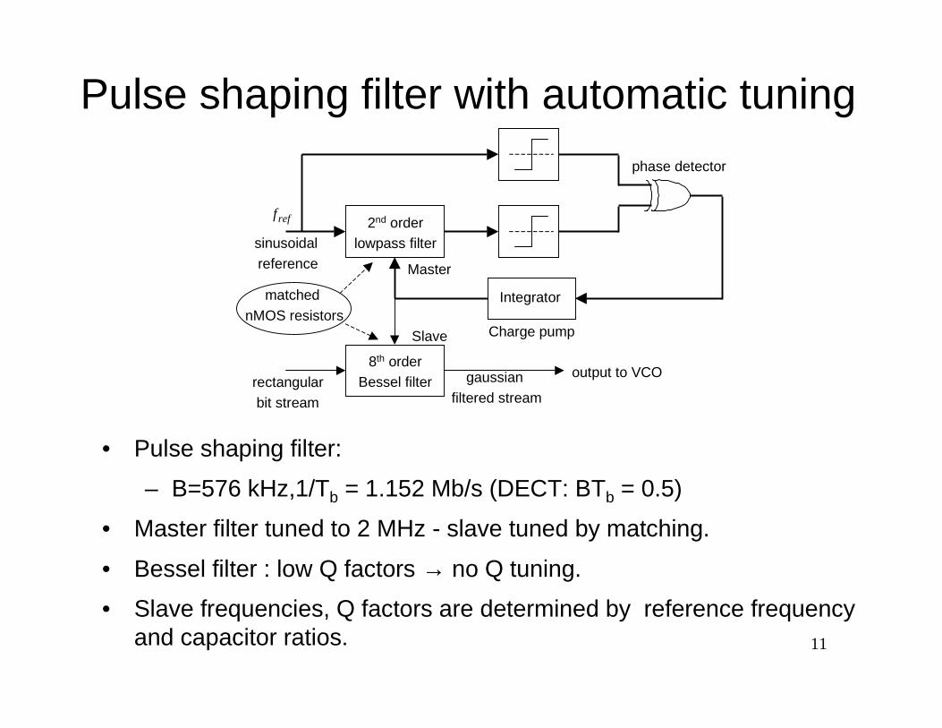
Pulse shaping filter with automatic tuning
• Pulse shaping filter:
– B=576 kHz,1/Tb = 1.152 Mb/s (DECT: BTb = 0.5)
• Master filter tuned to 2 MHz - slave tuned by matching.
• Bessel filter : low Q factors → no Q tuning.
• Slave frequencies, Q factors are determined by reference frequencyand capacitor ratios.
8th orderBessel filter
2nd orderlowpass filter
Integrator
sinusoidal reference
rectangular bit stream
gaussian filtered stream
phase detector
reff
Master
Slave
matched nMOS resistors
output to VCO
Charge pump
12
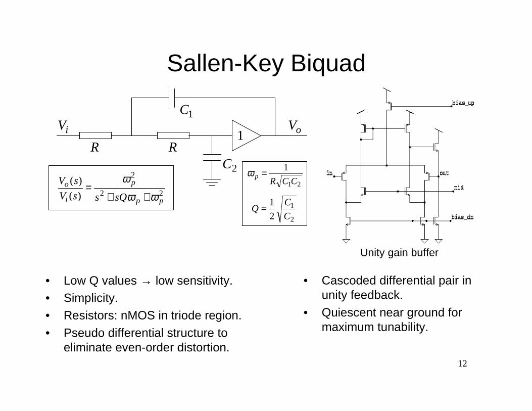
• Low Q values → low sensitivity.• Simplicity.• Resistors: nMOS in triode region.
• Pseudo differential structure toeliminate even-order distortion.
• Cascoded differential pair inunity feedback.
• Quiescent near ground formaximum tunability.
R
2C
1C
1iV oV
R
21
1
CCRp =ω
2
1
2
1
C
CQ =
22
2
)(
)(
pp
p
i
o
sQssV
sV
ωω
ω
++=
Sallen-Key Biquad
Unity gain buffer
13
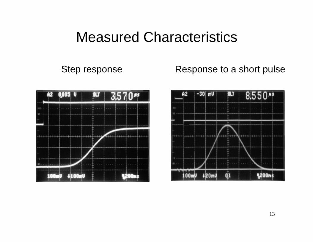
Step response Response to a short pulse
Measured Characteristics
14
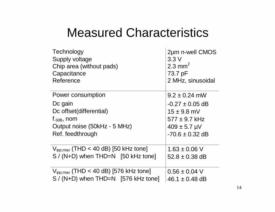
Measured CharacteristicsTechnology 2µm n-well CMOSSupply voltage 3.3 VChip area (without pads) 2.3 mm2
Capacitance 73.7 pFReference 2 MHz, sinusoidal
Power consumption 9.2 ± 0.24 mWDc gain -0.27 ± 0.05 dBDc offset(differential) 15 ± 9.8 mVf-3dB, nom 577 ± 9.7 kHzOutput noise (50kHz - 5 MHz) 409 ± 5.7 µVRef. feedthrough -70.6 ± 0.32 dB
Vipp,max (THD < 40 dB) [50 kHz tone] 1.63 ± 0.06 VS / (N+D) when THD=N [50 kHz tone] 52.8 ± 0.38 dB
Vipp,max (THD < 40 dB) [576 kHz tone] 0.56 ± 0.04 VS / (N+D) when THD=N [576 kHz tone] 46.1 ± 0.48 dB
15
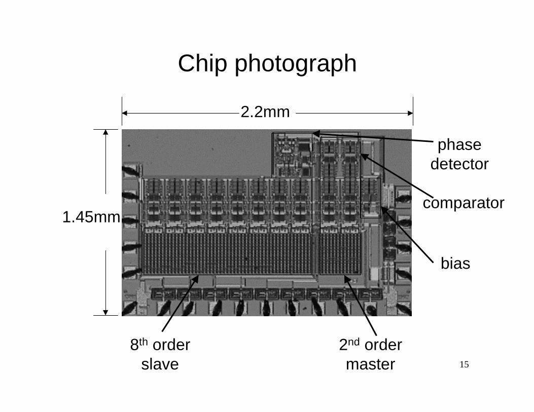
1.45mm
8th orderslave
2.2mm
2nd ordermaster
bias
comparator
phasedetector
Chip photograph
16
• A method for analog gaussian pulse shaping isproposed.
• Power and area savings over the existing method forhigh bit rates.
• Simulations demonstrate that DECT spectralspecifications are satisfied.
• Pulse shaping chip with automatic tuning is fabricated.
• Measurement results are given.
Conclusions