A Basical Study on Two-point Seismic Ray Tracing

Wenzheng Yang

December 16, 2003

Abstract

In this report, the raypath equation is deduced by using plane wavetheory and making high frequency approximation. Two kinds of two-pointseismic ray tracing iterative nonlinear methods(the Shooting method andthe Bending method) are discussed. The Shooting method fixes one endand apply the raypath equation to find the ray path. The Bending methodfixes both ends and use Fermat’s principle to find the right ray path. TheBending method is more efficient than the Shooting method. To area withcomplex velocity structure, the results of ray tracing relocation show thata small variation of location could produce large differences in travel time.

1 Introduction

In seismology, we study the propagation of seismic wave from source to receiversin order to locate the source and study the structure of the earth. In geomet-rical optics, we study the propagation of light wave. Both the movement ofseismic wave and light wave obey the same physical laws (e.g. Snell law, Huy-gens’ principle), so we can apply the well-developed methods in optics to studyseismic wave.Ray is a geometrical vector, with the direction of wave propagation. A ray isfixed if the source point, receive point and the incident angle are fixed. TheFermat’s principle governs the geometry of raypaths. In computer graphics, thedefination of ray tracing is: “ A technique to create realistic images by calcu-lating the paths taken by rays of light entering the observer’s eye at differentangles.” [2]. In seismology, ray tracing is based on the concept that seismicenergy of infinitely high frequency follows a trajectory determined by the raytracing equations. Physically, these equations describe how energy continues inthe same direction until it is refracted by velocity variations [8].The essential problem of earthquake location is to solve the ray equations builtbetween source and receive points. This problem could be expressed as a two-point ray tracing problem and had been studied by many authors ([4],[9]).Mathematically, this problem could be treated as a two-point initial value orboundary value problem and solved by finite-difference methods. In the follow-ing, I will review that how the problem is set up and discuss several methodswidely used.

1

2 The Raypath Equation

For plane waves in three spatial dimensions, we can write displacement har-monic solutions to the wave equation as:

u = A(x)ei(ωt±k·x) (1)

where k is a wavevector specifying the direction of propagation and thus, is aray. Equation (1) satisfies wave equation, which is:

52u =1

c2(x)u, (2)

where c(x) is either the local P-wave speed, or the local S-wave speed. Followingthe derivation by Lay and Wallace [5], I modify equation (1) to be:

u = A(x)eiω(W (x)/c0−t), (3)

where W (x) · ω/c0 replaces k · x, is a function of position, and c0 is a referencevelocity. Bring equation (3) into (2), we haven two sets of equations:

52A(x)−A(x)ω2

c20

3∑i=1

[W (x),i ]2 =ω2

c2(x)A(x), (4)

23∑

i=1

W (x),i A(x),i +A(x)52 W (x) = 0. (5)

To equation (4), we can make an approximation that 52A(x)A(x) → 0, which is very

accurate for short-period (high frequencies). Then we arrival at the eikonalequation

3∑i=1

(∂W (x)

∂xi)2 =

c20

c(x)2. (6)

From the defination, we know that W (x) = c0x

c(x) = c0T , where T is raytravel-time. So, we can rewrite equation (6) to be:

(5T )2 =1

c(x)2, (7)

5T is the slowness vector of a ray path. Equation (6) is also called the equationsof travel time field. The waves under consideration are non-dispersive in thehigh frequency approximation [1]. Let the distance of ray path be s, measuredalong the ray, we have:

dxds

= c(x)5 T = unit vector. (8)

With equation (8), we can eliminate the time quantity in equation (7), and getthe following raypath equation:

d

ds(

1c(x)

dxds

) = 5(1

c(x)). (9)

2

3 The Shooting Method

Figure 1. Illustration of the Bending and the Shooting methods (from [11]).

As shown in figure 1b, the shooting method fixes one end of the ray path( source point), and takes initial incidence angle i0 and initial azimuth j0,and then uses raypath equation to find the coordinates of another end point(station).Equation (9) could be rewriten as first-order equations

∂x∂s

= c(x)p, (10)

∂p∂s

=∂

∂s(

1c(x)

). (11)

Where p is the slowness. Equation (10) and (11) give a system of six firstorder ODE (ord. dif. equ.) equations (can be simplified into five independentequations) which must be integrated numerically to find the ray path ([4]).For Cartesian Coordinates, the system becomes

x′ = c sin i cos j;y′ = c sin i sin j;z′ = c cos i;i′ = − cos i[cxcosj + cy sin j] + cz sin i;

j′ =1

sin i[cx sin j − cy cos j].

The solution should satisfy

h(i0, j0) = H, (12)

3

g(i0, j0) = G. (13)

Here h and g are the calculated coordinates (lat. and lon.) of the end of theray. H and G are the coordinates of the end of the desired ray [4].Newton’s method and False Position method are used to solve equation (12)and (13), and both methods have to be applied iteratively.The Newton’s method:[

∂h∂i0

∂h∂j0

∂g∂i0

∂g∂j0

] [i(n+1)0 − in0

j(n+1)0 − jn

0

]=

[H − hn

G− gn

]

The False Position method:∣∣∣∣∣∣∣k0 − k

(1)0 k0 − k

(2)0 k0 − k

(3)0

h(1) −H h(2) −H h(3) −H

g(1) −G g(2) −G g(3) −G

∣∣∣∣∣∣∣ = 0, (k = i, j)

The superscripts represents three previous estimates [4].The False Positionmethod does not need to calculate the ”variational equation” (partical deriva-tives), which has to be calculated in the Newton’s method. But it is expectedto converge more slowly.

4 The Bending Method

As shown in figure 1a, the bending method fixes the two ends, and takes someinitial estimate of the ray path and perturbs it until it satisfies a minimumtravel-time criterion.Consider a ray travelling from A to B through an inhomogenous medium withvelocity c and slowness p. The travel time, TB

A is given by:

TBA =

∫ B

A

ds

c, (14)

where ds is the arc length along the ray measured from some arbitrary pointand the integral is taken along the true ray path [4]. The ray path could beparameterized in Cartesian coordinates as :

x = x(q), y = y(q), z = z(q). (15)

So,ds

dq=

√x2 + y2 + z2 ≡ F, x =

∂x

∂q(16)

and the travel time becomes

TBA =

∫ qB

qA

pFdq. (17)

The travel time could be made stationary by standard methods of the calculusof variations. Here we can use the Euler equations to summarized the whole

4

problem:

d

dq(pF )x = (pF )x,

d

dq(pF )y = (pF )y,

dF

dq= 0, (18)

with boundary conditions:

x(0) = xA, y(0) = yA, z(0) = zA,

x(1) = xB , y(1) = yB, z(1) = zB .

Where (pF )x = ∂∂x(pF ) and (pF )x = ∂

∂x(pF ). Here q ≡ sL , where L is the total

length of the ray path from A to B. So at A, q = 0 and q = 1 at B.For the (n + 1)-th iteration we have :

x(n+1) = x(n) + ξ(n) (19)

The criterion used for convergence is that the RMS path perturbation betweensuccessive iterations, given by

E(n) = [∫ 1

0|ξ(n)(q)|2dq]

12 , (20)

be less than a given value comparable with the round-off error [4].

5

5 discussion

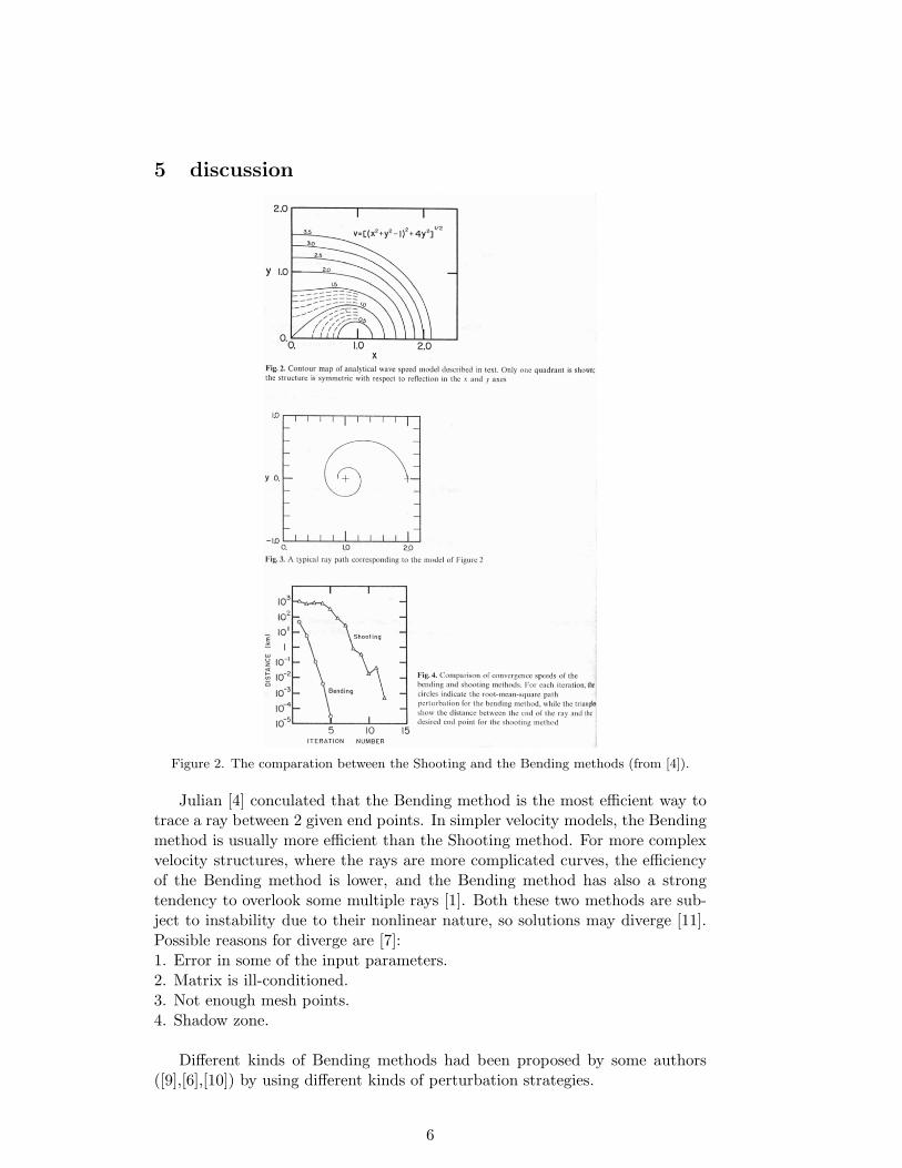
Figure 2. The comparation between the Shooting and the Bending methods (from [4]).

Julian [4] conculated that the Bending method is the most efficient way totrace a ray between 2 given end points. In simpler velocity models, the Bendingmethod is usually more efficient than the Shooting method. For more complexvelocity structures, where the rays are more complicated curves, the efficiencyof the Bending method is lower, and the Bending method has also a strongtendency to overlook some multiple rays [1]. Both these two methods are sub-ject to instability due to their nonlinear nature, so solutions may diverge [11].Possible reasons for diverge are [7]:1. Error in some of the input parameters.2. Matrix is ill-conditioned.3. Not enough mesh points.4. Shadow zone.

Different kinds of Bending methods had been proposed by some authors([9],[6],[10]) by using different kinds of perturbation strategies.

6

Engdahl and Lee [3] had used the ray tracing method (shooting method) torelocate regional earthquakes across the San Andreas fault, where the velocitystructure is very complex (figure 3). They found that small change of locationmay produce large differences in travel time.

Figure 3. The change of ray-paths caused by small change of location (from [3]).

References

[1] Cerveny, V., Ray tracing algorithms in three-dimensional laterally verying lay-ered structures, “Seismic tomography”,99-133, D.Reidel Publishing Company,1987.

[2] http://dictionary.reference.com/

[3] Engdahl, E. R. and W. H. K. Lee, Relocation of local earthquakes by seismicray tracing, J. G. R., 81, 4400-4406, 1976.

[4] Julian, B. R. and D. Gubblins, Three-dimensional seismic ray tracing, J. Geo-phys. , 43, 95-113, 1977.

[5] Lay, T. and T. C. Wallace, “Modern global seismology”, 71-74, Academic Press,1995.

[6] Moser, T. J., G. Nolet and R. Snieder, Ray bending revisited, B.S.S.A., 82,259-288, 1992.

[7] Pereyra, V., W. H. K. Lee and H. B. Keller, Solving two-point seismic-ray tracingproblems in a heterogeneous medium, B.S.S.A. ,70, 79-99, 1980.

[8] Vidale J. E., Finite-difference calculation of travel time, B.S.S.A. , 78, 2062-2076,1988.

7

[9] Um, J. and C. H. Thurber, A fast algorithm for two-point seismic ray tracing,B.S.S.A. , 77, 972-986, 1987.

[10] Sun, Y., Ray tracing in 3-D media by parameterized shooting, it Geophys. J.Int., 114, 145-155, 1993.

[11] Thurber, C. H. and E. Kissling, Advances in Travel-Time Calculations for 3-D structures, “Advances in Seismic Event Location”, 71-99, Kluwer AcademicPublishers, 2000.

8