Pergamon Computers Math. Applic. Vol. 36, No. 3, pp. 33-53, 1998

@ 1998 Elsevier Science Ltd. All rights reserved Printed in Great Britain

PII: SO898-1221(98)00127-8 08981221/98 $19.00 + 0.00

A Basis-Deficiency-Allowing Variation of the Simplex Method for Linear Programming

P.-Q. PAN Department of Applied Mathematics

Southeast University, Nanjing 210096, P.R. China

(Received November 199’7; accepted December 1997)

Abstract-h one of the most important and fundamental concepts in the simplex methodology, basis is restricted to being a square matrix of the order exactly equal to the number of rows of the coefficient matrix. Such inflexibility might have been the source of too many zero steps taken by the simplex method in solving real-world linear programming problems, which are usually highly degen- erate. To dodge this difficulty, we first generalize the basis to allow the deficient case, characterized as one that has columns fewer than rows of the coefficient matrix. Variations of the primal and dual simplex procedures are then made, and used to form a two-phase method based on such a basis, the number of whose columns varies dynamically in the solution process. Generally speaking, the more degenerate a problem to be handled is, the fewer columns the basis will have; so, thii renders the possibility of efficiently solving highly degenerate problems. We also provide a valuable insight into the distinctive and favorable behavior of the proposed method by reporting our computational experiments. @ 1998 Elsevier Science Ltd. All rights reserved.

Keywords-Linear programming, Simplex method, Degeneracy, Basis deficiency, Least squares problem, Orthogonal transformation.

1. INTRODUCTION

1997 marked the golden anniversary of linear programming and the simplex method, founded by Dantzig [1,2]. As perhaps the most beneficial and widely used mathematical tools in technology and science, linear programming, and the simplex method might be well accepted to be one of man’s greatest achievements in this century.

Effects of degeneracy were noted as early as nearly at the beginning of the fruitful and exciting period of 50 years [3,4]. The problem with degeneracy is that basic variables bearing value zero could lead to zero-length steps and, as a result, undermine the finiteness of the simplex method. Although authors make a nondegeneracy assumption to guarantee the finiteness of the simplex method, degeneracy occurs all the time in practice. In fact, it is common that a considerable proportion of basic variables bear value zero.

Yet, from a practical point of view, finiteness of the simplex method is not a problem, since there is not much chance of cycling practically, even in the presence of degeneracy. Bather, the real problem caused by it is stalling: the methods can become stuck at a degenerate vertex for too long a time before exiting it, and consequently consume too much time, or fail to solve diicult large- scale LP problems entirely. Although the perturbation method [5] and the lexicographic rule (61 (which coincide in spirit), and Bland’s rules (71 prevent cycling, their computational performance is unsatisfactory. In spite of alternatives for handling degeneracy having been cropped up from time to time, it remains troublesome in practice (also see, for example, [8-131).

33

34 P.-Q. PAN

In view of these facts, we believe that significant progress is impossible unless degeneracy is dodged completely, or to some extent at least, and that as a step toward the realization of this aim, a generalization of the basis, one of the most important and fundamental concepts in the simplex methodology, is absolutely necessary.

But how to do so? Conventionally, basis is a nonsingular square submatrix from the coefficient matrix, of order

exactly equal to the number of rows of the coefficient matrix. As a result, in literature the coefficient matrix is always assumed to have full row rank although it is not the case in general. Essentially, degeneracy occurs if and only if the right-hand side of the equality constraint is included in a subspace, spanned by some proper subset of the basis’s columns. In this case, the basic variables corresponding to columns that are not included in the proper subset vanish unavoidably. To remedy this fault, therefore, these columns should be dropped from the basis; it is noted that through doing so, there would be no basic variable bearing value of zero at all, and hence, a strictly positive steplength could be taken, if the subset is a smallest one of such kind.

Motivated by the preceding ideas, in this paper we make an attempt to allow deficient basis, characterized as one that has columns fewer than rows of the coefficient matrix. Generally speaking, the more degenerate a problem to be solved is, the fewer columns the basis should have in the process. For the first time, consequently, a high degree of degeneracy could contribute to method’s efficiency.

In the next section, we first generalize the basis to include the deficient case. Then, in Section 3, we make a variation of the primal simplex procedure using such a basis, the number of whose columns changes dynamically in the process while maintaining primal feasibility, until an optimal basis is reached. In Section 4, we make a variation of the dual simplex method too. In Section 5, we propose a general purpose method, based on the procedures established in the foregoing two sections, and highlight important pivot criterion issues. Finally, in Section 6, we provide some valuable insight into the distinctive and favorable behavior of the proposed method by reporting numerical results of our computational trials.

2. THE GENERALIZATION OF BASIS

Approaches to solving various LP problems can be well presented with problems in the following standard form:

min cTz, (2.la)

s.t. Ax=b, (2.lb)

x 2 6, (2.lc)

where A E 7ZmX” with m < n, and b E Rm, c E I?‘. It is assumed that the cost vector c, the right-hand side b, and A’s columns and rows are all nonzero, and that (2.lb) is consistent. In addition, we stress that no assumption is made on the rank of A, except 1 < rank(A) I m.

The following notation will be used throughout:

oj the jth column of A, ei the unit vector with the ith component 1, ??j the jth component of a vector ??,

11 ??11 the a-norm of a vector ??, R(o) the range space of a matrix ??.

We begin with redefining the basis.

DEFINITION 2.1. A basis is submatrix consisting of any linearly independent set of A’s columns, whose range space includes b.

Obviously, the preceding is more general than the conventional definition of basis. Thereby, bases may be classified into the following two categories.

Basis-Deficiency-Allowing Variation 35

DEFINITION 2.2. If the number of basis’ columns equals the number of rows of the coefficient matrix, it is normal basis; else, it is deficient basis.

Clearly, any m linearly independent columns from A comprise a normal basis. And the simplex method and existing variants of it merely use the normal basis.

Let B be a basis with ml columns and let N be nonbasis, consisting of the remaining columns. Define the ordered basic and nonbasic (index) sets respectively by

JE = 01 ,...,jmll and JN = {kl,. . . > k-ml), (2.2)

where ji, i = 1,. . . ,ml, istheindexoftheith columnofB, and kj,j = l,...,n-ml, the index of the jth column of N. The subscript of a basic index ji is called TOW index, and that of a nonbasic index kj column index. Components of 2 and c, and columns of A, corresponding to basic and nonbasic indices, are called basic and nonbatic, respectively. Hereafter, for simplic- ity of exposition, components of vectors and columns of matrices will always be arranged, and partitioned conformably, as the ordered set { JB, JN} changes. For example, we have

Thus, program (2.1) can be written

(2.3a)

(2.3b)

(2.3~)

And, accordingly, the dual program will be

max b' y,

s-t* [;++ [;;I = [;;I 7

ZB, ZN 10.

(2.4a)

(2.4b)

(2.4~)

The primal or dual simplex method can be used to solve program (2.1), as far as the basis is normal (ml = m) throughout. For example, a pair of complementary primal and dual basic solutions can be determined, respectively, from (2.3b) and (2.4b), that is,

z,=o and IB = B-lb (2.5)

and

g = B-T~B, (2.6a)

.ZN=CN--N~~~, and EB =o. (2.6b)

When the basis is deficient, however, the preceding formulas, and conventional iterations are not well defined. Therefore, new methods have to be found to cope with the generalized basis introduced previously.

36 P.-Q. PAN

3. THE PRIMAL PROCEDURE

In this section, we make a variation of the primal simplex method, based on the generalized basis. In the process, the number of basis’s columns varies dynamically, as it is updated iteration by iteration while maintaining primal feasibility, until optimality is achieved.

For simplicity, we shall use the system’s augmented matrix to represent the system itself. So, for any nonsingular matrix QT E Rmxm, [QTB, QTiV, QTb] is equivalent to [B,iV,b], in the sense of their representing the same constraint (2.lb). In particular, an orthogonal matrix QT can be determined such that QTB E Rmxml is upper triangular. In this case, the [QTB, QTN, QTb] is said to be canonical (augmented) matrix. Notably, since B is a basis, all diagonal entries of QTB are nonzero, while all the last m - ml components, if any, of QTb are zero.

Let us develop a tableau version of the primal procedure first. Assume the presence of a canonical matrix, which might as well be denoted again by [B, N, b], with the associated sets JB and JN known. Assume ml < m, and put program (2.1) into the following equivalent tableau, by appending the cost row to [B, N, b], as partitioned:

B N

CTB

b = “d c; 0

1-i

;2 “d 1 3 CL CA 0 (3.1)

where B1 E Rmlxml is in the tableau below:

upper triangular. Accordingly, the dual program of (3.1) can be written

From (3.1), a primal basic solution can be determined immediately:

Li?N=o, (3.3a)

fg = B,‘bl, (3.3b)

corresponding to the objective value f = CL B,’ bl. And a basic solution to (3.2) can be obtained, that is,

ZN = cN - N,TBF~c~,

(3.4 a)

(3.4 b)

,%i=J = 0. (3.4 c)

The preceding 3 and E clearly exhibit complementary slackness. We shall regard (3.4) as a “dual basic solution”, since it is a basic solution to the original dual program of (2.1), except g is different from its correspondent by only an orthogonal matrix factor (the same below).

The ZN can be obtained alternatively. In fact, it is easy to show that annihilating by Gaussian elimination the basic entries of the cost row of (3.1) renders EN and f as well

Bl NI bl 0 N2 O2 . 0 z; -f 1 (3.5)

The preceding is called canonical tableau. Take a single iteration. Assume that the current canonical tableau, say (3.5), is primally

feasible, i.e., ZB 1 0. If, in addition, it holds that ,?hr 1 0, then primal and dual optimal solutions are already obtained, and hence all is done. Suppose that this is not the case. We

Be&Deficiency-Allowing Variation 37

select a nonbasic column to enter the basis in accordance with some column selection criteria, for instance, Dantzig’s original one below:

q= Argmin{Zkj ]j=l,...,n-ml}. (3.6)

So, zkk4 c 0, and the nonbasic column Uk, will enter the basis. There will be one of the following two possibilities arising, which should be handled differently.

CASE 1. ml = m, or ml < m but the (ml + 1) through mth components of ck, are all zero. Clearly, this case occurs if and only if ck, E R(B). In this case, the value of the nonbasic

variable Zk, of the solution is allowed to increase from zero with the objective value decreasing. To determine a blocking basic variable, compute the ml-vector

v = B+ikq, (3.7)

by solving the upper triangular system Blv = &kq, where ?Lks is the subvector consisting of the first ml components of ak,. There is no blocking variable, and the program is hence lower unbounded if the row index set below is empty:

I = {i ] vi > 0, i = 1,. . . , ml}. (3.3)

If, otherwise, it is nonempty, then the row index p may be determined such that

a = Z-i = min ;J ($1 iEI}>O, where the inequality holds under nondegeneracy, i.e., 3~3 > 0. Therefore, as the value of the nonbasic variable Xk, increases from zero up to (Y with values of the other nonbasic variables unchanged, the value of “cj, decreases from 2j, down to zero while primal feasibility remains unaltered. This leads to the following formula for updating the basic feasible solution 3’:

2.. *= 2.. -au. 3x * 3% z, vi=1 ,..., ml, %k, :=a. (3.10)

Then we bring the pth basic column of the canonical tableau to the end of its nonbasic columns (corresponding to N), with JB and JN adjusted conformably. If p = ml, the resulting B E 7PX(m1-1) is already upper triangular, while when p < ml, the B is an upper Hessenberg with nonzero subdiagonal entries in its p through (ml - l)th columns. These unwanted entries are zeroed by premultiplying [B, N, b] in (3.5) by a series of appropriate Givens rotations. Afterwards, the qth nonbasic column of (3.5) is brought to the end of its basic columns, with JB and JN adjusted conformably. It is easy to show that the new B E Rmxml, or B1 E Rmlxml is again upper triangular, with nonzero diagonal entries.

At first thought, one might expect that a column to be chosen to enter a basis rarely happens to be in the basis’ range space, and hence this case rarely occurs. However, our computational experiments indicate quite the contrary, as will be shown in Section 6.

CASE 2. ml < m and some of the (ml + 1) through mth components of ck, are nonzero. The case occurs if and only if ck, $! R(B). This time, the value of the nonbasic variable zk,

is not allowed to increase from zero because this action will lead to violation of some of the last m - ml constraints. So, we annihilate the (ml + 2) through mth components of ck, by premultiplying [B, N, b] by an appropriate Householder reflection, and bring the qth nonbasic column of the canonical tableau (3.5) to the end of its basic part. Then we set ml := ml + 1, and rearrange JB and JN conformably. It is obvious that the resulting B is an m x ml upper triangular matrix with nonzero diagonal entries.

Clearly, the orthogonal transformations carried out in either case do not disturb zero com- ponents of b’s subvector 02 at all. When the newly-entering entry of the cost row is zeroed

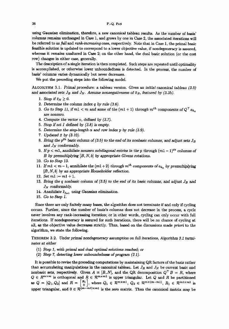
38 P.-Q. PAN

using Gaussian elimination, therefore, a new canonical tableau results. As the number of basis’ columns remains unchanged in Case 1, and grows by one in Case 2, the associated iterations will be referred to as fvll and mnlc-increasing ones, respectively. Note that in Case 1, the primal basic feasible solution is updated to correspond to a lower objective value, if nondegeneracy is assured, whereas it remains unaltered in Case 2; on the other hand, the dual basic solution (or the cost row) changes in either case, generally.

The description of a single iteration is then completed. Such steps are repeated until optima& is accomplished, or otherwise lower unboundedness is detected. In the process, the number of basis’ columns varies dynamically but never decreases.

We put the preceding steps into the following model.

ALGORITHM 3.1. Primal procedure: a tableau version. Given an initial canonical tableau (3.5) and associated sets JB and JN. Assume nonnegativeness of Zg, featured by (3.3b).

1. StopifzN 10. 2. Determine the column index q by rule (3.6). 3. Go to Step 11, if ml C m and some of the (ml + 1) through mth components of QT ak,

are nonzero. 4. Compute the vector v, defined by (3.7). 5. Stop if set I defined by (3.8) is empty. 6. Determine the step-length Q and row index p by rule (3.9). 7. Updated 5 by (3.10). 8. Bring the pth basic column of (3.5) to the end of its nonbasic columns, and adjust sets JB

and JN conformably. 9. If p < ml, annihilate nonzero subdiagonal entries in the p through (ml - l)th columns of

B by premultiplying [B, N, b] by appropriate Givens rotations. 10. Go to Step 13. 11. If ml < m - 1, annihilate the (ml + 2) through mth components of ak, by premultiplying

[B, N, b] by an appropriate Householder reflection. 12. Set ml := ml + 1. 13. Bring the q nonbasic column of (3.5) to the end of its basic columns, and adjust JB and

JN conformably. 14. Annihilate Zj,,,, using Gaussian elimination. 15. Go to Step 1.

Since there are only finitely many bases, the algorithm does not terminate if and only if cycling occurs. Further, since the number of basis’s columns does not decrease in the process, a cycle never involves any rank-increasing iteration; or in other words, cycling can only occur with full iterations. If nondegeneracy is assured for such iterations, there will be no chance of cycling at all, as the objective value decreases strictly. Thus, based on the discussions made priori to the algorithm, we state the following.

THEOREM 3.2. Under primal nondegeneracy assumption on full iterations, Algorithm 3.1 termi- nates at either

(1) Step 1, with primal and dual optimal solutions reached; or (2) Step 7, detecting lower unboundedness of program (2.1).

It is possible to revise the preceding computations by maintaining QR factors of the basis rather than accumulating manipulations in the canonical tableau. Let JB and JN be current basic and nonbasic sets, respectively. Given A z (B, IV], and the QR decomposition QT B = R, where QERmXrn is orthogonal and R E Rmxml is upper triangular. Let Q and R be partitioned as Q = [Ql,Qz] and R = [ 21, where Q1 E 7Zmxm1, Qz E 7?“‘X(m-m1), RI E Rmlxml is

upper triangular, and 0 E 7Z(m-m1)xm1 is the zero matrix. Then the canonical matrix may be

Basis-Deficiency-Allowing Variation 39

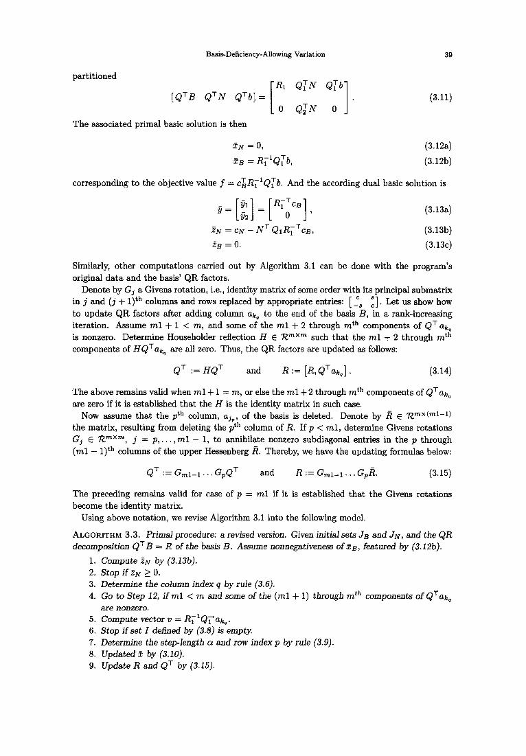
partitioned

[QTB QTiV QTb] = [“d s; 1”]. (3.11)

The associated primal basic solution is then

zN=o, (3.12a)

ZB = R;‘Q;b, (3.12b)

corresponding to the objective value f = cLR;~QT~. And the according dual basic solution is

g= [;;I = [Rpq) (3.13a)

ZN = CN - NT Q~RY~cB, (3.13b)

Zg = 0. (3.13c)

Similarly, other computations carried out by Algorithm 3.1 can be done with the program’s original data and the basis’ QR factors.

Denote by Gj a Givens rotation, i.e., identity matrix of some order with its principal submatrix in j and (j + l)th columns and rows replaced by appropriate entries: [ -“, 61. Let us show how to update QR factors after adding column akq to the end of the basis B, in a rank-increasing iteration. Assume ml + 1 < m, and some of the ml + 2 through mth components of QT akq is nonzero. Determine Householder reflection H E Rmxm such that the ml + 2 through mth components of HQTakq are all zero. Thus, the QR factors are updated as follows:

QT := HQT and R := [R, Q’ak,] . (3.14)

The above remains valid when ml + 1 = m, or else the ml + 2 through mth components of QTak, are zero if it is established that the H is the identity matrix in such case.

Now assume that the pth column, aj,,, of the basis is deleted. Denote by i? E RmX(ml-l) the matrix, resulting from deleting the pth column of R. If p < ml, determine Givens rotations Gj E 7Zmxn, j = p,..., ml - 1, to annihilate nonzero subdiagonal entries in the p through (ml - l)th columns of the upper Hessenberg R. Thereby, we have the updating formulas below:

QT := Gml-l.. . G,QT and R := G,l-l . . . G& (3.15)

The preceding remains valid for case of p = ml if it is established that the Givens rotations become the identity matrix.

Using above notation, we revise Algorithm 3.1 into the following model.

ALGORITHM 3.3. Primd procedure: a revised version. Given initial sets JB and JN, and the QR decomposition QTB = R of the basis B. Assume nonnegativeness of ZB, featured by (3.12b).

1. 2. 3. 4.

5. 6. 7. 8. 9.

Compute ,?N by (3.13b). Si$Op if EN 2 0. Determine the column index q by rule (3.6). Go to Step 12, if ml < m and some of the (ml + 1) through mth components of QTak, are nonzero. Compute vector v = RTIQiak,. Stop if set I defined by (3.8) is empty. Determine the step-length Q and row index p by rule (3.9). Updated z by (3.10). Update R and QT by (3.15).

40

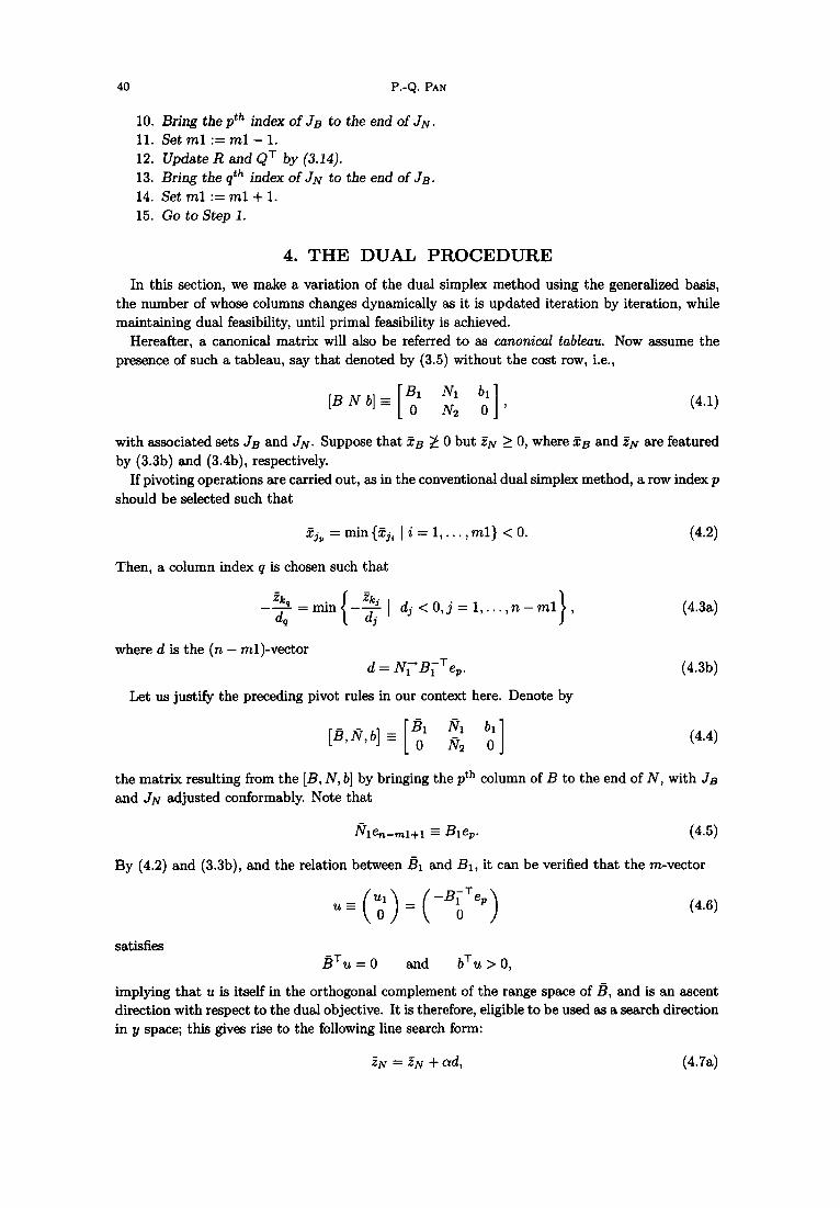
10. 11. 12. 13. 14. 15.

P.-Q. PAN

Bring the pth index of JB to the end of JN. Set ml := ml - 1. Update R and QT by (3.14). Bring the qth index of JN to the end of JB. Set ml := ml + 1. Go to Step 1.

4. THE DUAL PROCEDURE

In this section, we make a variation of the dual simplex method using the generalized basis, the number of whose columns changes dynamically as it is updated iteration by iteration, while maintaining dual feasibility, until primal feasibility is achieved.

Hereafter, a canonical matrix will also be referred to as canonical ta6leau. Now assume the presence of such a tableau, say that denoted by (3.5) without the cost row, i.e.,

(4.1)

with associated sets JB and JN. Suppose that Zg 2 0 but ZN 2 0, where IB and ZN are featured by (3.3b) and (3.4b), respectively.

If pivoting operations are carried out, as in the conventional dual simplex method, a row index p should be selected such that

Q,=min{fj< Ii=l,...,ml}<O.

Then, a column index q is chosen such that

(4.2)

zk -2 = min

d, 1 -2 1 dj <O,~=l,...~~-~l}~ (4.3a)

3

where d is the (n - ml)-vector d = NiBTTeP.

Let us justify the preceding pivot rules in our context here. Denote by

(4.3b)

[BJ$] 3 Bl [

fll 61 0 iv2 0 1

(4.4)

the matrix resulting from the [B, N, b] by bringing the pth column of B to the end of N, with JB and JN adjusted conformably. Note that

Nlen-ml+l = Ble,. (4.5)

By (4.2) and (3.3b), and the relation between & and Bl, it can be verified that the m-vector

(4.6)

satisfies BTu=O and bTu > 0,

implying that u is itself in the orthogonal complement of the range space of B, and is an ascent direction with respect to the dual objective. It is therefore, eligible to be used as a search direction in y space; this gives rise to the following line search form:

&=EN+ad, (4.7a)

Basis-Deficiency-Allowing Variation 41

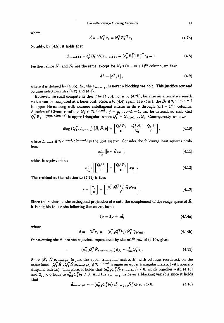
where

Notably, by (4.5), it holds that

(4.7b)

(4.8)

Further, since Ni and Ni are the same, except for fii’s (n - m + l)th column, we have

dT = [dT, l] ) (4.9)

where d is defined by (4.3b). So, the Zk,,_ml+l is never a blocking variable. This justifies row and column selection rules (4.2) and (4.3).

However, we shall compute neither d by (4.3b), nor d^ by (4.7b), because an alternative search vector can be computed at a lower cost. Return to (4.4) again. If p c ml, the & E 7P1X(m1-1) is upper Hessenberg with nonzero subdiagonal entries in its p through (ml - l)th columns. A series of Givens rotations Gj E Rmlxml, j = p, . . . , ml - 1, can be determined such that QT& E Rm’x(mi-1) is upper triangular, where QT = Gmi-i . . . GP. Consequently, we have

(4.10)

where Im_mi E 7Z(m-m1)x(m-m1) is th e unit matrix. Consider the following least squares prob- lem:

n&r+-BzslJ, (4.11)

which is equivalent to

The residual at the solution to (4.11) is then

T= (ekQ&) Qleml

0

(4.12)

(4.13)

Since the T above is the orthogonal projection of b onto the complement of the range space of B, it is eligible to use the following line search form:

(4.14a)

where 6= -#Tri = - (eL,QTbi) fiTQie,i.

Substituting the Z into the equation, represented by the mlth row of (LLIO), gives

(4.14b)

(4.15)

Since [&,#ie,_,i+i] is just the upper triangular matrix BI with columns reordered, on the other hand, [Qr&, QT&en-,,,i+i] E 7Pixm1 is again an upper triangular matrix (with nonzero diagonal entries). Therefore, it holds that (e~lQT&e,+mi+i) # 0, which together with (4.15) and Ij, < 0 leads to e:iQTbi # 0. And the zk,_,l+l is never a blocking variable since it holds that

(4.16)

42 P.-Q. PAN

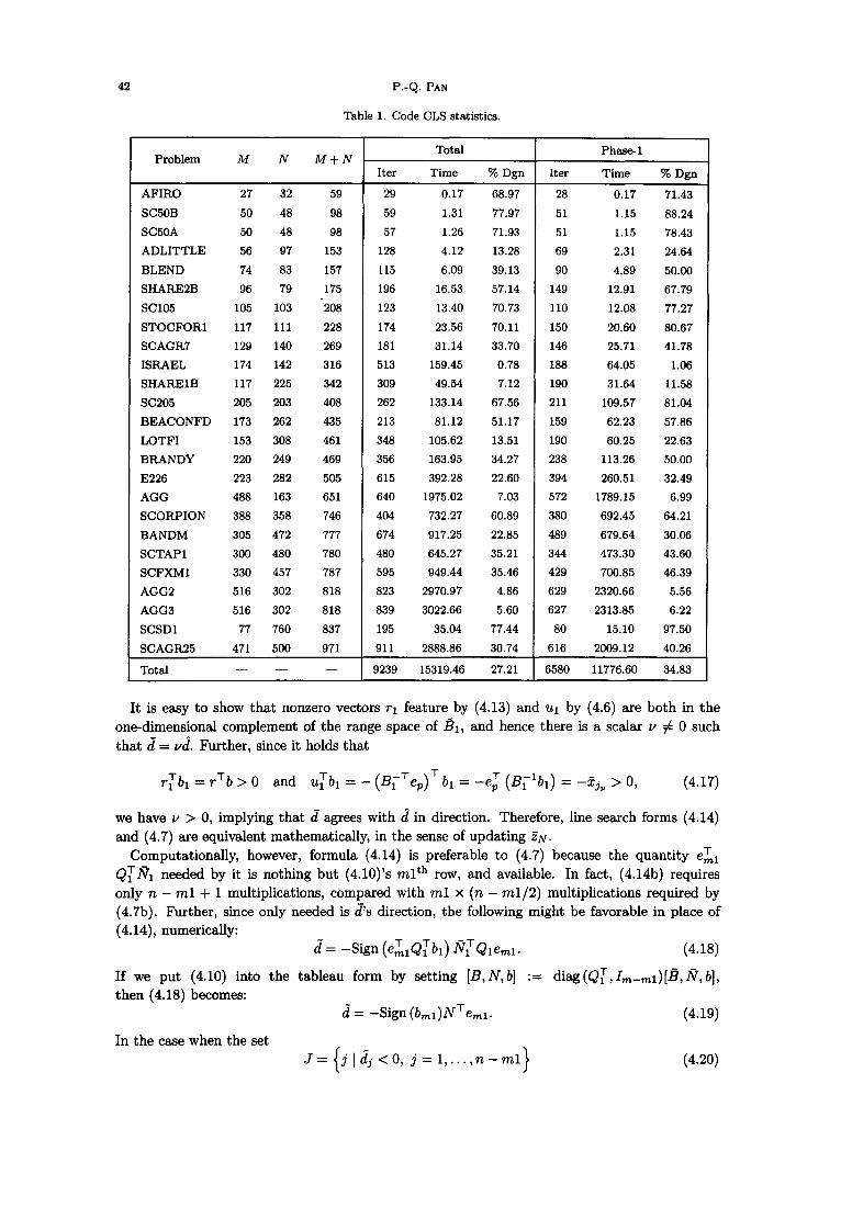
Table 1. Code CLS statistics.

Total Problem M N M+N

Phase-1

Iter Time % Dgn Iter Time % Dgn

AFIRO 27 32 59 29 0.17 68.97 28 0.17 71.43

SCBOB 50 48 98 59 1.31 77.97 51 1.15 88.24

SC50A 50 48 98 57 1.26 71.93 51 1.15 78.43

ADLITTLE 56 97 153 128 4.12 13.28 69 2.31 24.64

BLEND 74 83 157 115 6.09 39.13 90 4.89 50.00

SHARESB 96 79 175 196 16.53 57.14 149 12.91 67.79

SC105 105 103 ‘208 123 13.40 70.73 110 12.08 77.27

STOCFORl 117 111 228 174 23.56 70.11 150 20.60 80.67

SCAGR7 129 140 269 181 31.14 33.70 146 25.71 41.78

ISRAEL 174 142 316 513 159.45 0.78 188 64.05 1.06

SHARElB 117 225 342 309 49.54 7.12 190 31.64 11.58

SC205 205 203 408 262 133.14 67.56 211 109.57 81.04

BEACONFD 173 262 435 213 81.12 51.17 159 62.23 57.86

LOTFI 153 308 461 348 105.62 13.51 190 60.25 22.63

BRANDY 220 249 469 356 163.95 34.27 238 113.26 50.00

E226 223 282 505 615 392.28 22.60 394 260.51 32.49

AGG 488 163 651 640 1975.02 7.03 572 1789.15 6.99

SCORPION 388 358 746 404 732.27 60.89 380 692.45 64.21

BANDM 305 472 777 674 917.25 22.85 489 679.64 30.06

SCTAPl 300 480 780 480 645.27 35.21 344 473.30 43.60

SCFXMl 330 457 787 595 949.44 35.46 429 700.85 46.39

AGG2 516 302 818 823 2970.97 4.86 629 2320.66 5.56

AGG3 516 302 818 839 3022.66 5.60 627 2313.85 6.22

SCSDl 77 760 837 195 35.04 77.44 80 15.10 97.50

SCAGR25 471 500 971 911 2888.86 30.74 616 2009.12 40.26

Total - - - 9239 15319.46 27.21 6580 11776.60 34.83

It is easy to show that nonzero vectors r-1 feature by (4.13) and ui by (4.6) are both in the one-dimensional complement of the range space of &, and hence there is a scalar Y # 0 such that d = vd. Further, since it holds that

rTbi = rTb > 0 and ~lbi = - (B;TeP)T bi = -ep’ (Br’bi) = -Ij, > 0, (4.17)

we have v > 0, implying that d agrees with d^ in direction. Therefore, line search forms (4.14) and (4.7) are equivalent mathematically, in the sense of updating ??N.

Computationally, however, formula (4.14) is preferable to (4.7) because the quantity e:i QTni needed by it is nothing but (4.10)‘s mlth row, and available. In fact, (4.14b) requires only n - ml + 1 multiplications, compared with ml x (n - m1/2) multiplications required by (4.7b). Further, since only needed is & direction, the following might be favorable in place of (4.14)) numerically:

2 = -Sign (eL,QTbi) sTQie,i. (4.18)

If we put (4.10) into the tableau form by setting [B, N,b] := diag(QT,I,_,i)[B, w, b], then (4.18) becomes:

d = -Sign (b,i)N’e,i. (4.19)

In the case when the set J= jI&<O, j=l,...,n-ml

> (4.20)

BasisDekiency-Allowing Variation

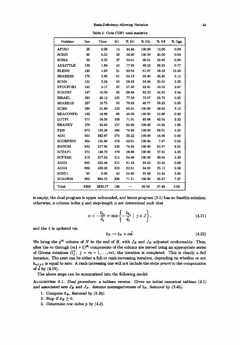
Table 2. Code CDPl total statietice.

Problem Iter Time Ml %Ml % Dfc % Nfl % Dgn

AFIRO 25 0.06 12 44.44 100.00 12.00 0.00

SCSOB 60 0.33 28 56.80 100.00 20.00 0.00

SCWA 59 0.33 27 54.61 96.61 16.95 0.00

ADLITTLE 130 1.60 43 77.95 49.23 56.92 0.77

BLEND 120 1.65 51 69.54 61.67 38.33 12.50

SHAHESB 176 3.95 61 64.13 95.45 45.45 5.11

SC105 131 3.24 59 56.63 94.66 20.61 2.29

STOCFORl 145 5.17 67 57.50 92.41 19.31 2.07

SCAGR7 197 10.00 85 66.48 82.23 34.52 2.54

ISRAEL 393 28.12 135 77.58 75.57 55.73 0.25

SHAFlElB 287 16.75 93 79.65 40.77 59.23 0.35

SC205 286 31.69 123 60.01 100.00 29.02 3.15

BEACONFD 140 18.89 69 40.05 100.09 12.86 0.00

LOTFI 271 34.55 108 71.01 85.98 43.54 3.32

BRANDY 370 45.92 127 65.99 100.00 54.05 1.89

E226 672 102.38 166 74.86 100.00 68.01 4.02

AGG 561 243.87 274 56.22 100.00 14.08 0.36

SCORPION 364 135.66 178 50.01 100.00 7.97 0.55

BANDM 632 217.56 226 74.35 100.00 52.37 6.01

SCTAPl 374 148.79 170 56.66 100.00 27.01 4.55

SCFXMl 519 217.62 212 64.49 100.00 38.54 5.20

AGG2 665 422.44 315 61.19 93.53 22.41 0.60

AGG3 689 436.05 322 62.51 94.05 25.11 0.58

SCSDl 90 9.00 43 55.90 95.56 14.44 5.56

SCAGR25 853 684.75 336 71.51 100.00 45.37 7.27

Total 8209 2820.37 199 - 93.09 37.46 3.06

is empty, the dual program is upper unbounded, and hence program (2.1) has no feasit otherwise, a column index q and step-length CK are determined such that

43

)le solution;

(4.21)

and the E is updated via ??N := &7 + ad (4.22)

We bring the qth column of N to the end of B, with JB and JN adjusted conformably. Thus, after the m through (ml + l)th components of the column are zeroed using an appropriate series of Givens rotations GT, j = m - l,... ,ml, the iteration is completed. This is clearly a full iteration. The next can be either a full or rank-increasing iteration, depending on whether or not bml+l is equal to zero. A rank-increasing one will not include the steps priori to the computation of d’by (4.19).

The above steps can be summarized into the following model.

ALGORITHM 4.1. Dual procedure: a tablesu version. Given an initial csnonicaI tableau (4.1) and associated sets JB and JN. Assume nonnegativeness of EN, featured by (3.4b).

1. Compute j?B, featured by (3.3b). 2. Stop if zg 2 0. 3. Determine row index p by (4.2).

44 P.-Q. PAN

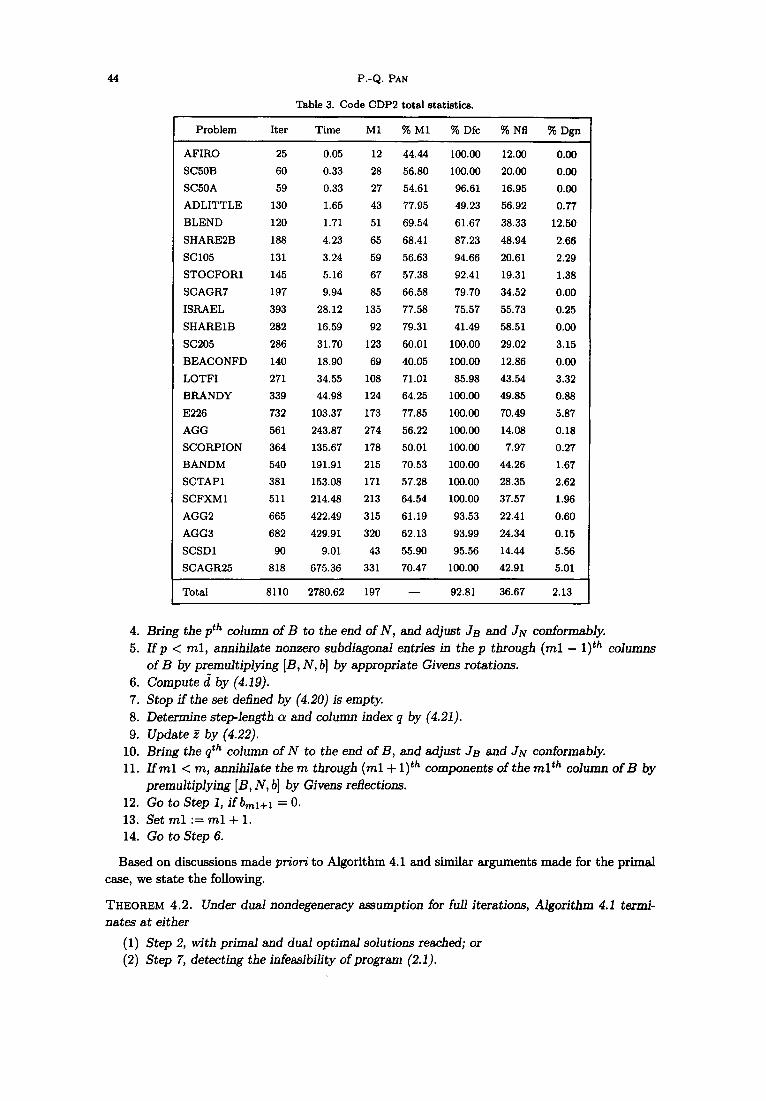
Table 3. Code CDP2 total statistics.

Problem Iter Time Ml % Ml % Dfc % Nfl % Dgn

AFIRO 25 0.05 12 44.44 100.00 12.00 0.00

SCBOB 60 0.33 28 56.80 100.00 20.00 0.00

SC50A 59 0.33 27 54.61 96.61 16.95 0.00

ADLITTLE 130 1.65 43 77.95 49.23 56.92 0.77

BLEND 120 1.71 51 69.54 61.67 38.33 12.50

SHAREZB 188 4.23 65 68.41 87.23 48.94 2.66

SC105 131 3.24 59 56.63 94.66 20.61 2.29

STOCFORl 145 5.16 67 57.38 92.41 19.31 1.38

SCAGR’I 197 9.94 85 66.58 79.70 34.52 0.00

ISRAEL 393 28.12 135 77.58 75.57 55.73 0.25

SHARElB 282 16.59 92 79.31 41.49 58.51 0.00

SC205 286 31.70 123 60.01 100.00 29.02 3.15

BEACONFD 140 18.90 69 40.05 100.00 12.86 0.00

LOTFI 271 34.55 108 71.01 85.98 43.54 3.32

BRANDY 339 44.98 124 64.25 100.00 49.85 0.88

E226 732 103.37 173 77.85 100.00 70.49 5.87

AGG 561 243.87 274 56.22 100.00 14.08 0.18

SCORPION 364 135.67 178 50.01 100.00 7.97 0.27

BANDM 540 191.91 215 70.53 100.00 44.26 1.67

SCTAPl 381 153.08 171 57.28 100.00 28.35 2.62

SCFXMl 511 214.48 213 64.54 100.00 37.57 1.96

AGG2 665 422.49 315 61.19 93.53 22.41 0.60

AGG3 682 429.91 320 62.13 93.99 24.34 0.15

SCSDl 90 9.01 43 55.90 95.56 14.44 5.56

SCAGR25 818 675.36 331 70.47 100.00 42.91 5.01

Total 8110 2780.62 197 - 92.81 36.67 2.13

4. 5.

6. 7. 8. 9.

10. 11.

12. 13. 14.

Bring the pth column of B to the end of N, and adjust JB and JN conformably. If p < ml, annihilate nonzero subdiagonal entries in the p through (ml - l)th columns of B by premultiplying [B, N, b] by appropriate Givens rotations. Compute 2 by (4.19). Stop if the set defined by (4.20) is empty. Determine step-length Q and column index q by (4.21). Update Z by (4.22). Bring the qth column of N to the end of B, and adjust JB and JN conformably. If ml < m, annihilate the m through (ml + l)th components of the mlth column of B by premultiplying [B, N, b] by Givens reflections. Go to Step 1, if b,l+l = 0. Set ml := ml + 1. Go to Step 6.

Based on discussions made priori to Algorithm 4.1 and similar arguments made for the primal case, we state the following.

THEOREM 4.2. Under dual nondegeneracy assumption for full iterations, Algorithm 4.1 termi- nates at either

(1) Step 2, with primal and dual optimal solutions reached; or (2) Step 7, detecting the infeasibility of program (2.1).

Basis-Deficiency-Allowing Variation

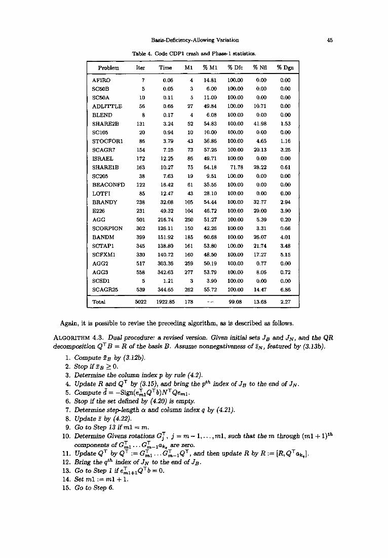
Table 4. Code CDPl cresh and Phaeel statistics.

45

Again, it is possible to revise the preceding algorithm, as is described as follows.

Problem Iter Time Ml %Ml % Dfc % Nfl %Dgn

AFIRO 7 0.06 4 14.81 100.00 0.00 0.00

SCBOB 5 0.05 3 6.00 100.00 0.00 0.00

SC50A 10 0.11 5 11.00 100.00 0.00 0.00

ADLITTLE 56 0.66 27 49.84 100.00 10.71 0.00

BLEND 8 0.17 4 6.08 100.00 0.00 0.00

SHAHESB 131 3.24 52 54.83 100.00 41.98 1.53

SC105 20 0.94 10 10.00 100.00 0.00 0.00

STOCFORl 86 3.79 43 36.86 100.00 4.65 1.16

SCAGR’I 154 7.25 73 57.26 100.00 20.13 3.25

ISRAEL 172 12.25 86 49.71 100.00 0.00 0.00

SHAHElB 163 10.27 75 64.18 71.78 28.22 0.61

SC205 38 7.63 19 9.51 100.00 0.00 0.00

BEACONFD 122 16.42 61 35.55 100.00 0.00 0.00

LOTFI 85 12.47 43 28.10 100.00 0.00 0.00

BRANDY 238 32.08 105 54.44 100.00 32.77 2.94

E226 231 49.32 104 46.72 100.00 29.00 3.90

AGG 501 216.74 250 51.27 100.00 5.39 0.20

SCORPION 302 126.11 150 42.26 100.00 3.31 0.66

BANDM 399 151.92 185 60.68 100.00 26.07 4.01

SCTAPl 345 138.80 161 53.80 100.00 21.74 3.48

SCFXMl 330 140.72 160 48.50 100.00 17.27 5.15

AGG2 517 303.36 259 50.19 100.00 0.77 0.00

AGG3 558 342.63 277 53.79 100.00 8.06 0.72

SCSDl 5 1.21 3 3.90 100.00 0.00 0.00

SCAGH.25 539 344.65 262 55.72 100.00 14.47 6.86

Total 5022 1922.85 178 - 99.08 13.68 2.27

ALGORITHM 4.3. Dual procedure: a revised version. Given initisl sets JB and JN, and the QR decomposition QT B = R of the basis B. Assume nonnegativeness of i?N, featured by (3.13b).

1. 2. 3. 4. 5. 6. 7. 8. 9.

10.

11. 12. 13. 14. 15.

Compute ZB by (3.12b). Stop if 5, 2 0. Determine the column index p by rule (4.2). Update R and QT by (3.15), and bring the pth index of JB to the end of JN. Compute d = -Sign(eL,QTb)NTQe,l. Stop if the set defined by (4.20) is empty. Determine steplength cy and column index q by (4.21). Update E by (4.22). Go to Step 13 if ml = m. Determine Givens rotations GT, j = m - 1, . . . ,ml, such that the m through (ml + l)th components of GL, . . . GA_,ak, are zero. Update QT by QT := GL, . . . GL_,QT, and then update R by R := [R, QTak,]. Bring the qth index of JN to the end of JB. Go to Step 1 if ez,+IQTb = 0. Set ml := ml + 1. Go to Step 6.

P.-Q. PAN

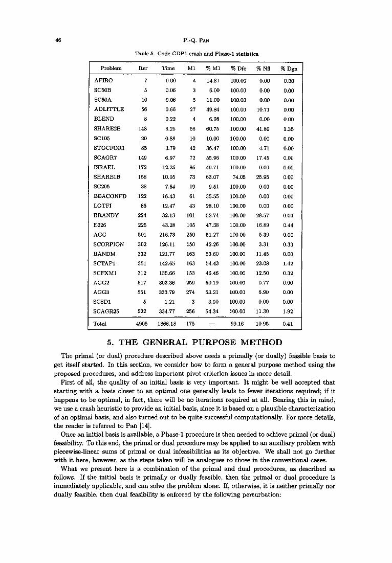
Table 5. Code CDPl crash and Phase1 statistics

Problem Iter Time Ml % Ml % Dfc % Nfl % Dgn

AFIRO 7 0.00 4 14.81 100.00 0.00 0.00

SCSOB 5 0.06 3 6.00 100.00 0.00 0.00

SCBOA 10 0.06 5 11.00 100.00 0.00 0.00

ADLITTLE 56 0.66 27 49.84 100.00 10.71 0.00

BLEND 8 0.22 4 6.08 100.00 0.00 0.00

SHARE2B 148 3.25 58 60.75 100.00 41.89 1.35

SC105 20 0.88 10 10.00 100.00 0.00 0.00

STOCFORl 85 3.79 42 36.47 100.00 4.71 0.00

SCAGRT 149 6.97 72 55.96 100.00 17.45 0.00

ISRAEL 172 12.25 86 49.71 100.00 0.00 0.00

SHARElB 158 10.05 73 63.07 74.05 25.95 0.00

SC205 38 7.64 19 9.51 100.00 0.00 0.00

BEACONFD 122 16.43 61 35.55 100.00 0.00 0.00

LOTFI 85 12.47 43 28.10 100.00 0.00 0.00

BRANDY 224 32.13 101 52.74 100.00 28.57 0.00

E226 225 43.28 105 47.38 100.00 16.89 0.44

AGG 501 216.73 250 51.27 100.00 5.39 0.00

SCORPION 302 126.11 150 42.26 100.00 3.31 0.33

BANDM 332 121.77 163 53.60 100.00 11.45 0.00

SCTAPl 351 142.65 163 54.43 100.00 23.08 1.42

SCFXMl 312 135.66 153 46.46 100.00 12.50 0.32

AGG2 517 303.36 259 50.19 100.00 0.77 0.00

AGG3 551 333.79 274 53.21 100.00 6.90 0.00

SCSDl 5 1.21 3 3.90 100.00 0.00 0.00

SCAGR25 522 334.77 256 54.34 100.00 11.30 1.92

Total 4905 1866.18 175 - 99.16 10.95 0.41

5. THE GENERAL PURPOSE METHOD The primal (or dual) procedure described above needs a primally (or dually) feasible basis to

get itself started. In this section, we consider how to form a general purpose method using the proposed procedures, and address important pivot criterion issues in more detail.

First of all, the quality of an initial basis is very important. It might be well accepted that starting with a basis closer to an optimal one generally leads to fewer iterations required; if it happens to be optimal, in fact, there will be no iterations required at all. Bearing this in mind, we use a crash heuristic to provide an initial basis, since it is baaed on a plausible characterization of an optimal basis, and also turned out to be quite successful computationally. For more details, the reader is referred to Pan [14].

Once an initial basis is available, a Phase-l procedure is then needed to achieve primal (or dual) feasibility. To this end, the primal or dual procedure may be applied to an auxiliary problem with piecewise-linear sums of primal or dual infeasibilities as its objective. We shall not go further with it here, however, as the steps taken will be analogues to those in the conventional cases.

What we present here is a combination of the primal and dual procedures, as described as follows. If the initial basis is primally or dually feasible, then the primal or dual procedure is immediately applicable, and can solve the problem alone. If, otherwise, it is neither primally nor dually feasible, then dual feasibility is enforced by the following perturbation:

Basis-Deficiency-Allowing Variation

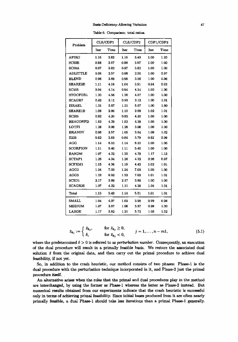
Table 6. Comparison: total ratios.

Problem CLS/CDPl CLS/CDPZ CDPl/CDPZ

Iter Time Iter Time Iter Time

AFIRC 1.16 2.83 1.16 3.40 1.06 1.20

SC50B 0.98 3.97 0.98 3.97 1.00 1.00

SC5OA 0.97 3.82 0.97 3.82 1.00 1.00

ADLITTLE 0.98 2.57 0.98 2.50 1.00 0.97

BLEND 0.96 3.69 0.96 3.56 1.00 0.96

SHARBZB 1.11 4.18 1.04 3.91 0.94 0.93

SC105 0.94 4.14 0.94 4.14 1.00 1.00

STOCFORl 1.20 4.56 1.20 4.57 1.00 1.00

SCAGR7 0.92 3.11 0.92 3.13 1.00 1.01

ISRAEL 1.31 5.67 1.31 5.67 1.00 1.00

SHARElB 1.08 2.96 1.10 2.99 1.02 1.01

SC205 0.92 4.20 0.92 4.20 1.00 1.00

BEACONFD 1.52 4.29 1.52 4.29 1.00 1.00

LOTFI 1.28 3.06 1.28 3.06 1.00 1.00

BRANDY 0.96 3.57 1.05 3.64 1.09 1.02

E226 0.92 3.83 0.84 3.79 0.92 0.99

AGG 1.14 8.10 1.14 8.10 1.00 1.00

SCORPION 1.11 5.40 1.11 5.40 1.00 1.00

BANDM 1.07 4.22 1.25 4.78 1.17 1.13

SCTAP 1 1.28 4.34 1.26 4.22 0.98 0.97

SCFXMl 1.15 4.36 1.16 4.43 1.02 1.01

AGG2 1.24 7.03 1.24 7.03 1.00 1.00

AGG3 1.22 6.93 1.23 7.03 1.01 1.01

SCSDl 2.17 3.89 2.17 3.89 1.00 1.00

SCAGR25 1.07 4.22 1.11 4.28 1.04 1.01

Total 1.13 5.43 1.14 5.51 1.01 1.01

SMALL 1.04 4.07 1.03 3.98 0.99 0.98

MEDIUM 1.07 3.87 1.06 3.87 0.99 1.00

LARGE 1.17 5.62 1.21 5.71 1.03 1.02

47

zkj := 'kj Y for zkj 10,

6, for zkj < 0, j = l,...,n-ml, (5.1)

where the predetermined 6 > 0 is referred to ES perttlrbution number. Consequently, an execution of the dual procedure will result in a primally feasible basis. We restore the associated dual solution E from the original data, and then carry out the primal procedure to achieve dual feasibility, if not yet.

So, in addition to the crash heuristic, our method consists of two phases: Phase-l is the dual procedure with the perturbation technique incorporated in it, and Phase-2 just the primal procedure itself.

An alternative arises when the roles that the primal and dual procedures play in the method are interchanged, by using the former as Phase-l whereas the latter as Phase-2 instead. But numerical results obtained from our experiments indicate that the crash heuristic is successful only in terms of achieving primal feasibility. Since initial bases produced from it are often nearly primally feasible, a dual Phase-1 should take less iterations than a primal Phase-l generally.

48 P.-Q. PAN

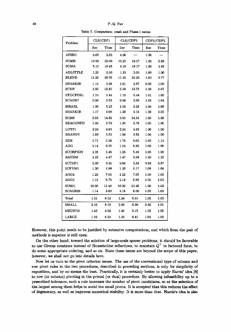
Table 7. Comparison: crash and Phase-1 ratios.

Problem CLS/CDPl CLS/CDPZ CDPl/CDP2

Iter Time Iter Time Iter Time

AFIRO 4.00 2.83 4.00 - 1.00 -

SC50B 10.20 23.00 10.20 19.17 1.00 0.83

SC50A 5.10 10.45 5.10 19.17 1.00 1.83

ADLITTLE 1.23 3.50 1.23 3.50 1.00 1.00

BLEND 11.25 28.76 11.25 22.23 1.00 0.77

SHARE2B 1.14 3.98 1.01 3.97 0.89 1.00

SC105 5.50 12.85 5.50 13.73 1.00 1.07

STOCFOR.1 1.74 5.44 1.76 5.44 1.01 1.00

SCAGR7 0.95 3.55 0.98 3.69 1.03 1.04

ISRAEL 1.09 5.23 1.09 5.23 1.00 1.00

SHARElB 1.17 3.08 1.20 3.15 1.03 1.02

SC205 5.55 14.36 5.55 14.34 1.00 1.00

BEACONFD 1.30 3.79 1.30 3.79 1.00 1.00

LOTFI 2.24 4.83 2.24 4.83 1.00 1.00

BRANDY 1.00 3.53 1.06 3.53 1.06 1.00

E226 1.71 5.28 1.75 6.02 1.03 1.14

AGG 1.14 8.25 1.14 8.26 1.00 1.00

SCORPION 1.26 5.49 1.26 5.49 1.00 1.00

BANDM 1.23 4.47 1.47 5.58 1.20 1.25

SCTAPl 1.00 3.41 0.98 3.32 0.98 0.97

SCFXMl 1.30 4.98 1.38 5.17 1.06 1.04

AGGP 1.22 7.65 1.22 7.65 1.00 1.00

AGG3 1.12 6.75 1.14 6.93 1.01 1.03

SCSDl 16.00 12.48 16.00 12.48 1.00 1.00

SCAGR25 1.14 5.83 1.18 6.00 1.03 1.03

Total 1.31 6.12 1.34 6.31 1.02 1.03

SMALL 2.16 6.13 2.06 6.20 0.95 1.01

MEDIUM 1.43 4.92 1.46 5.15 1.03 1.05

LARGE 1.19 6.22 1.23 6.41 1.03 1.03

However, this point needs to be justified by extensive computations, and which from the pair of methods is superior is still open.

On the other hand, toward the solution of large-scale sparse problems, it should be favorable to use Givens rotations instead of Householder reflections, to maintain QT in factored form, to do some appropriate ordering, and so on. Since these issues are beyond the scope of this paper, however, we shall not go into details here.

Now let us turn to the pivot criterion issues. The use of the conventional type of column and row pivot rules in the two procedures, described in preceding sections, is only for simplicity of exposition, and by no means the best. Practically, it is certainly better to apply Harris’ idea [8] to row (or column) pivoting in the primal (or dual) procedure. By allowing infeasibility up to a prescribed tolerance, such a rule increases the number of pivot candidates, so as the selection of the largest among them helps to avoid too small pivots. It is accepted that this reduces the effect of degeneracy, as well as improves numerical stability. It is more than that. Harris’s idea is also

Basis-Deficiency-Allowing Variation

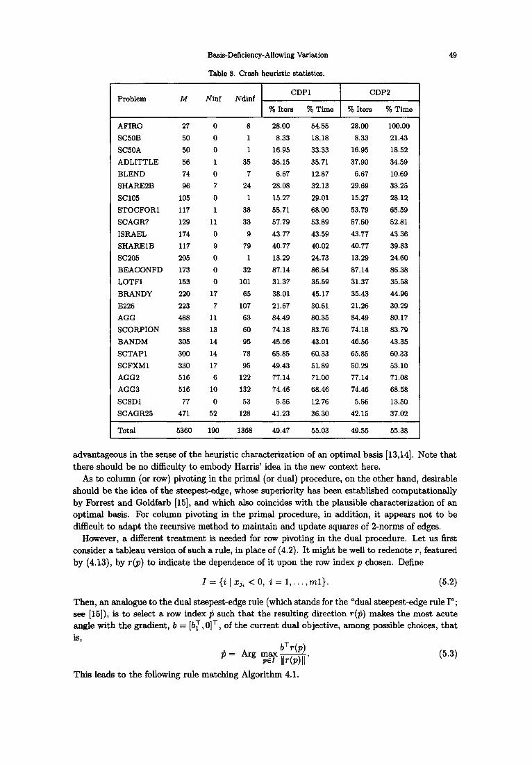
Table 8. Crash heuristic statistics.

49

r CDPl CDP2 Problem M Ninf Ndinf .

% Iters % Time % Iters % Time

AFIRO 27 0 8 28.00 54.55 28.00 100.00

SC50B 50 0 1 8.33 18.18 8.33 21.43

SCSOA 50 0 1 16.95 33.33 16.95 18.52

ADLITTLE 56 1 35 36.15 35.71 37.90 34.59

BLEND 74 0 7 6.67 12.87 6.67 10.69

SHARESB 96 7 24 28.08 32.13 29.69 33.25

SC105 105 0 1 15.27 29.01 15.27 28.12

STOCFOFU 117 1 38 55.71 68.00 53.79 65.59

SCAGR7 129 11 33 57.79 53.89 57.50 52.81

ISRAEL 174 0 9 43.77 43.59 43.77 43.36

SHARElB 117 9 79 40.77 40.02 40.77 39.83

SC205 205 0 1 13.29 24.73 13.29 24.60

BEACONFD 173 0 32 87.14 86.54 87.14 86.38

LOTFI 153 0 101 31.37 35.59 31.37 35.58

BRANDY 220 17 65 38.01 45.17 35.43 44.96

E226 223 7 107 21.67 30.61 21.26 30.29

AGG 488 11 63 84.49 80.35 84.49 80.17

SCORPION 388 13 60 74.18 83.76 74.18 83.79

BANDM 305 14 95 45.66 43.01 46.56 43.35

SCTAPl 300 14 78 65.85 60.33 65.85 60.33

SCFXMl 330 17 95 49.43 51.89 50.29 53.10

AGG2 516 6 122 77.14 71.00 77.14 71.08

AGG3 516 10 132 74.46 68.46 74.46 68.58

SCSDl 77 0 53 5.56 12.76 5.56 13.50

SCAGR25 471 52 128 41.23 36.30 42.15 37.02

Total 5360 190 1368 49.47 55.03 49.55 55.38

advantageous in the sense of the heuristic characterization of an optimal basis [13,14]. Note that there should be no difficulty to embody Harris’ idea in the new context here.

As to column (or row) pivoting in the primal (or dual) procedure, on the other hand, desirable should be the idea of the steepest-edge, whose superiority has been established computationally by Forrest and Goldfarb [15], and which also coincides with the plausible characterization of an optimal basis. For column pivoting in the primal procedure, in addition, it appears not to be difficult to adapt the recursive method to maintain and update squares of 2-norms of edges.

However, a different treatment is needed for row pivoting in the dual procedure. Let us first consider a tableau version of such a rule, in place of (4.2). It might be well to redenote T, featured by (4.13), by r(p) to indicate the dependence of it upon the row index p chosen. Define

I = {i 1 “ji < 0, i = 1,. . . ,ml}. (5.2)

Then, an analogue to the dual steepest-edge rule (which stands for the “dual steepest-edge rule I”; see [15]), is to select a row index $ such that the resulting direction r($) makes the most acute angle with the gradient, b = (br, OIT, of the current dual objective, among possible choices, that is,

Thii leads to the following rule matching Algorithm 4.1.

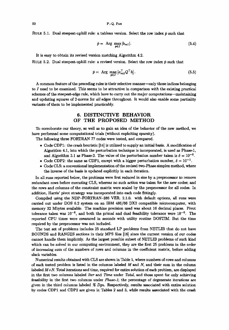
50 P.-Q. PAN

RULE 5.1. Dual steepest-uphill rule: a tableau version. Select the row index p such that

It is easy to obtain its revised version matching Algorithm 4.2.

RULE 5.2. Dual steepest-uphill rule: a revised version. Select the row index fi such that

(5.5)

A common feature of the preceding rules is their selective manner-only those indices belonging to I need to be examined. This seems to be attractive in comparison with the existing practical schemes of the steepest-edge rule, which have to carry out the major computations-maintaining and updating squares of 2-norms for all edges throughout. It would also enable some partiality variants of them to be implemented practicably.

6. DISTINCTIVE BEHAVIOR OF THE PROPOSED METHOD

To corroborate our theory, as well as to gain an idea of the behavior of the new method, we have performed some computational trials (without exploiting sparsity).

The following three FORTRAN 77 codes were tested, and compared.

?? Code CDPl: the crash heuristic [14] is utilized to supply an initial basis. A modification of Algorithm 4.1, into which the perturbation technique is incorporated, is used as Phase-l, and Algorithm 3.1 as Phe2. The value of the perturbation number taken is 6 = 10Bs.

??Code CDPZ: the same as CDPl, except with a bigger perturbation number, S = 10-l. ?? Code CLS: a conventional implementation of the revised two-Phase simplex method, where

the inverse of the basis is updated explicitly in each iteration.

In all runs reported below, the problems were first reduced in size by a preprocessor to remove redundant rows before executing CLS, whereas no such action was taken for the new codes; and the rows and columns of the constraint matrix were scaled by the preprocessor for all codes. In addition, Harris’ pivot strategy was incorporated into each code fittingly.

Compiled using the NDP-FORTRAN-386 VER. 2.1.0. with default options, all runs were carried out under DOS 6.2 system on an IBM 486/66 DX2 compatible microcomputer, with memory 32 Mbytes available. The machine precision used was about 16 decimal places. Pivot tolerance taken was lo-‘, and both the primal and dual feasibility tolerance were 10W6. The reported CPU times were measured in seconds with utility routine DOSTIM. But the time required by the preprocessor was not included.

The test set of problems includes 25 standard LP problems from NETLIB that do not have BOUNDS and RANGES sections in their MPS files [16] since the current version of our codes cannot handle them implicitly. As the largest possible subset of NETLIB problems of such kind which can be solved in our computing environment, they are the first 25 problems in the order of increasing sum of the numbers of rows and columns in the coefficient matrix, before adding slack variables.

Numerical results obtained with CLS are shown in Table 1, where numbers of rows and columns of each tested problem is listed in the columns labeled M and N, and their sum in the column labeled M+N. Total iterations and time, required for entire solution of each problem, are displayed in the first two columns labeled Iter and Time under TotaZ, and those spent for only achieving feasibility in the first two columns under Phase-l; the percentage of degenerate iterations are given in the third columns labeled % Dgn. Respectively, results associated with entire solution by codes CDPl and CDPP are given in Tables 2 and 3, while results associated with the crash

Basis-Deficiency-Allowing Variation 51

and Phase1 together in Tables 4 and 5. All runs terminated with the optimal objective values reached, as those in NETLIB index file.

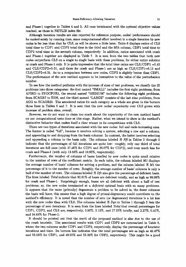
Although iteration results are also reported for reference purpose, codes’ performance should be ranked solely by running time, since computational effort involved in a single iteration by new codes is far less than that by CLS, as will be shown a little later. Table 6 displays ratios of CLS total time to CDPl and CDP2 total time in the third and the fifth column, CDPl total time to CDP2 total time in the seventh column, respectively. In addition, ratios associated with crash and Phase1 together are displayed in Table 7. It is seen from the two tables that both new codes outperform CLS on a single to single basis with these problems, for either entire solution or crash and Phase-l only. It is quite impressive that the total time ratios are CLS/CDPl =5.43 and CLS/CDP2=5.51, and those for crash and Phase-l are as high as CLS/CDP1=6.12 and CLS/CDP2=6.31. As to a comparison between new codes, CDP2 is slightly better than CDPl. The performance of the new method appears to be insensitive to the value of the perturbation number.

To see how the method performs with the increase of sizes of test problems, we classify the 25 problems into three categories: the first named “SMALL” includes the first eight problems, from AFIRO to STOCFORl, the second named “MEDIUM” includes the following eight problems, from SCAGR7 to E226, and the third named “LARGE” consists of the last nine problems, from AGG to SCAGR25. The associated ratios for each category as a whole are given in the bottom three lines in Tables 6 and 7. It is seen that the new codes’ superiority over CLS grows with increase of problem sizes, overall.

However, we do not want to claim too much about the superiority of the new method based on our computational tests done at this stage. Rather, what we intend to show is the method’s distinctive behavior that makes itself a clear winner in its competitions with CLS.

There are two types of iterations associated with the new codes: full and rank-increasing ones. The former is called “full,,, because it involves solving a system, selecting a row and a column, and appending to and dropping from the basis columns. In contrast, the latter involves selecting and appending a column to the basis only. The columns labeled % iVfl in Tables 2 through 5 indicate that the percentages of full iterations are quite low: roughly, only one third of total iterations are full ones (with 37.46% for CDPl and 36.67% for CDPZ), and even much less for crash and Phase1 (with only 13.68% and 10.95%) respectively).

Furthermore, the number of columns of bases handled by new codes is quite small relative to the number of rows of the coefficient matrix. In each table, the column labeled Ml displays the average number of basis’ columns for solving a problem, and the column labeled % Ml the percentage of it to the number of rows. Roughly, the average number of basis’ columns is only a half of the number of rows. The columns labeled % Dfc also give the percentage of deficient basis. The lines labeled Total indicate that 92.81% of bases are deficient totally, and as high as 99.08% for crash and Phase-l. Surprisingly enough, bases are all deficient with about a half of test problems; so, the new codes terminated at a deficient optimal basis with so many problems. It appears that the more (primally) degenerate a problem to be solved is, the fewer columns the basis will have; this means that a high degree of primal-degeneracy could contribute to the method’s efficiency. It is noted that the number of zero (or degenerate) iterations is a lot less with the new codes than with CLS. The columns labeled % Dgn in Tables 1 through 5 lists the percentage of zero iterations. It is seen from the lines labeled Total that overall percentages for CDPl, CDP2, and CLS are, respectively, 3.06%) 2.13%, and 27.21% totally, and 2.27%) 0.41%) and 34.83% for Phase-l.

It should be pointed out that the merit of the proposed method is also due to the use of the crash heuristic. The associated results with CDPl and CDP2 are summarized in Table 8, where the two columns under CDPl and CDPB, respectively, display the percentage of heuristic iterations and time. Its bottom line indicates that the total percentages are as high as 49.47% and 55.03% for CDPl, and 49.55% and 55.38% for CDP2, respectively. This might be a good

52 P.-Q. PAN

indication of the high computational efficiency of the proposed method. Moreover, the column labeled Ninfshows that the numbers of primal infeasibilities yielded from the heuristic are very low relative to problem sizes. In fact, primal feasibility was achieved with ten out of the 25 problems. It seems that the heuristic worked very well, though its capability for achieving dual feasibility is not as satisfactory as that for achieving primal feasibility, as is shown by the column labeled N&fin the table.

To conclude, the proposed basis-deficiency-allowing method does perform distinctively and favorably, and is very promising.

REFERENCES 1. G.B. Dantzig, Programming in a linear structure, Comptroller, USAF, Washington, D.C., (February 1948). 2. G.B. Dantzig, Programming of interdependent activities, II, Mathematical model, In Activity Analysis of

Production and Allocation, (Edited by T.C. Koopmans), pp. 19-32, John Wiley & Sons, New York, (1951); Ecomometrica, 17, (3,4), 200-211, (1949).

3. A.J. Hoffman, Cycling in the simplex algorithm, Report No. 2974, Nat. Bur. Standards, Washington, D.C., (1953).

4. E.M.L. Beale, Cycling in the dual simplex algorithm, Naval Research Logistics Quarterly 2, 269-275, (1955). 5. A. Charms, Optimality and degeneracy in linear programming, Econometricn 20, 160-170, (1952). 6. G.B. Dantzig, A. Orden and P. Wolfe, The generalized simplex method for minimizing a linear form under

linear inequality restraints, Pacific Journal of Mathematics 5, 183-195, (1955). 7. R.G. Bland, New finite pivoting rules for the simplex method, Mathematics of Operations Research 2, 103-

107, (1977). 8. P.M.J. Harris, Pivot selection methods of the Devex LP code, Mathematical Pmgnamming Study 4, 30-57,

(1975). 9. M. Benichou, J.M. Gauthier, G. Hentges and G. Ribiere, The efficient solution of linear programming

problems-Some algorithmic techniques and computational results, Mathematical Progmmming 18, 280- 322, (1977).

10. Scicon, Sciwnic/VM User Guide, Version 1.40, Scicon Limited, Milton Keynes, (1986). 11. B. Hattersley and J. Wilson, A dual approach to primal degeneracy, Mathematical Prognamming42, 135-145,

(1988). 12. P.E. Gill, W. Murray, M.A. Saunders and M.H. Wright, A practical anti-cycling procedure for linearly

constrained optimization, Mathematical Programming 45, 437-474, (1989). 13. P.-Q. Pan, Practical finite pivoting rules for the simplex method, Spektrum 1, 219-225, (1990). 14. P.-Q. Pan, A dual projective simplex method for linear programming, Computers Math. Applic. 85 (6),

119-135, (1998). 15. J.J.H. Forrest and D. Goldfarb, Steepest-edge simplex algorithms for linear programming, Mathematical

Pragnzmming 67, 341-374, (1992). 16. D.M. Gay, Electronic mail distribution of linear programming test problems, Mathematical Pmgmmming

Society COAL Newsletter 13, 10-12, (1985). 17. M. Bazarsa and J.J. Jarvis, Linear Programming and Network Flows, John Wiley & Sons, New York, (1977). 18. V. Chvatal, Linear Programming, &man and Company, San Francisco, CA, (1983). 19. G.B. Dantzig, Linear Progmmming and Extensions, Princeton University Press, Princeton, NJ, (1963). 20. S.-C. Fang and S. Puthenpura, Linear Optimization and Extensions: Theory and Algorithms, Prentice Hall,

(1993). 21. S.I. Gass, Linear Pmgmmming: Methods and Applications, Fifth edition, McGraw-Hill, New York, (1985). 22. D. Goldfarb and J.K. Reid, A practicable steepest-edge simplex algorithm, Mathematical Programming 12,

361371, (1977). 23. D. Goldfarb and M.J. Todd, Linear programming, in optimization, In Handbook in Opemtions Research and

Management Science, (Edited by G.L. Nemhauser and A.H.G. Rinnooy Kan), Volume 1, pp. 73-170, (1989). 24. G.H. Golub and C.F. Van Loan, Mat& Computations, John Hopkins Univenity Press, Baltimore, MD,

(1983). 25. H.-J. Greenberg, Pivot selection tactics, In Design and Implementation of Optimization Software, (Edited

by H.J. Greenberg), Sijthoff and Noordhoff, pp. 109-143, (1978). 26. D. Luemberger, Introduction to Linear and Nonlinear Pmgmmming, Addison-Wesley, Heading, MA, (1973). 27. K. Murty, Linear and Combinatorial Programming, John Wiley & Sons, New York, (1976). 28. W. Orchard-Hayes, Background development and extensions of the revised simplex method, Rand Report

HM 1433, The Rand Corporation, Santa Monica, CA, (1954). 29. P.-Q. Pan, A simplex-like method with bisection for linear programming, Optimization 5, 717-743, (1991). 30. P.-Q. Pan, Ratio-test-free pivoting rules for a dual Phase-1 method, In Proceedings of the Third Conference of

Chinese SIAM, (Edited by S.-T Xiao and F. Wu), pp. 245-249, Tsinghua University Press, Beijing, (1994a). 31. P.-Q. Pan, Achieving primal feasibility under the dual pivoting rule, Journal of Information d Optimization

Sciences 15 (3), 405-413, (1994b).

Basis-Deficiency-Allowing Variation 53

32. P.-Q. Pan, Composite phase-1 methods without measuring infeesibility, In Theory of Optimization and ite Applicatione, (Edited by M.-Y. Yue), pp. 359-364, Xidian University Press, Xian, (1994~).

33. P.-Q. Pan, New non-monotone procedurea for achieving dual feasibility, Journal of Nanjing University, Mathematics Biquarterly 13 (2), 155-162, (1995).

34. P.-Q. Pan, A modified bisection simplex method for linear programming, Journal of Computational Mathe- matica 14 (3), 249-255, (lQQ6).

35. P.-Q. Pan, The most-obtuse-angle row pivot rule for achieving dual feasibility: A computational study, European Journal of Opemtions Research 101 (l), 167-176, (1997).