A Bayesian approach to identify clay minerals from ...jtethys.org/wp-content/uploads/2013/10/Mollajan_et_al_2013.pdf · A Bayesian approach to identify clay minerals from petrophysical

Journal of Tethys: Vol.1, No. 1, 75-84

Mollajan et al., 2013 75 jtethys.org

A Bayesian approach to identify clay minerals from petrophysical logs in Gonbadly

Gas field, northeastern Iran

Amir Mollajan1, Mohammadali Sarparandeh

2, Fereydoon Sahabi

3, Gholamhossein Norouzi

4

1- M.Sc at Mining Exploration Engineering, School of Mining Engineering, University College of

Engineering, University of Tehran, Tehran, Iran.

2- M.Sc student of Petroleum Exploration Engineering, University College of Engineering, School of Mining Engineering, University of Tehran, Tehran, Iran. 3- Professor of Geology, School of Mining Engineering, University College of Engineering, University of

Tehran, Tehran, Iran.

4- Professor of Geophysics, School of Mining Engineering, University College of Engineering, University

of Tehran, Tehran, Iran.

* Corresponding Author: [email protected]

Abstract

More often clay matrix is the major factor to reduce the porosity and permeability in

sandstone facies. Consequently determination of clay minerals is of prime importance in

reservoir quality assessment. The present study aims to identify four different types of clay

mineral namely kaolinite, illite/cholorite, halloysite, and montmorilonite from

Petrophysical Logs (PLs) using Cation Exchange Capacity (CEC) parameter. In this

regard, PLs related to two wells of Shurijeh Formation (Early cretaceous) in Gonbadly gas

field, Northeast of Iran, were used. Utilizing measured CEC data and proper PLs, the CEC

log were generated by employing MLP neural network. Relying on this fact that clay

minerals can be classified based on their CEC value, the formation under study were

divided into five zones by implementing four cut offs on CEC log. Finally, Bayesian

classifier was applied on PLs to identify the desired zones. According to the obtained

results, the method proposed in this study is able to identify desired clay types with

average accuracy of 68.5% in single well analysis step and 65.75% for generalization step.

Keywords: Clay minerals, Cation Exchange Capacity (CEC), MLP neural network,

Bayesian classifier, Gonbadly oil field, Iran.

1- Introduction

Reservoir characterization is a

considerable process whose main

objective is identification and assessment

of reservoir productive zones and its

heterogeneities. Heterogeneities occur at

various scales because of variability in

lithology, pore fluids, clay content,

porosity, pressure and temperature

(Avseth et al., 2005). One of the main

items in reservoir characterization is

identifying clay minerals (Josh et al.,

2012). Today, various applications for

clay minerals has been found such as

ceramics and building materials, paper

industries, oil drilling, foundry moulds,

pharmaceuticals, and as adsorbents,

catalysts or catalyst supports, ion

exchangers, and decolorizing agents

(Zhang et al., 2010). There are wide

verity of methods for clay mineral

identification such as X-Ray-Diffraction

(XRD), Scanning Electron Microscope

(SEM) and Cation Capacity Exchange

(CEC). In this regard, CEC as an effective



method has not received much attention

yet and most studies related to its

performance are limited to agricultural

engineering. Nevertheless, CEC is

impressively employed in reservoir water

saturation estimation studies.

Hill and Milburn (1955 and 1979) were

the pioneers in this endeavor that showed

the excess conductivity caused by clay

minerals is related to cation capacity

exchange. Furthermore researches in this

area have led to providing a group of

formula for estimating of water saturation,

called CEC models. These models

consider the electrical conductivity of

clay minerals (Worthington, 1985), such

as the Waxman and Smits and dual water

models (Clavier et al., 1984). The

identification of the clay minerals can

take the form of multiple classification

process and their advantages. Different

classification methods can be easily

trained with known examples of previous

patterns and put to effective use of

solving unknown or untrained instances

of the problem.

The present study aims to identify

different clay minerals utilizing

experimental measurements of CEC and

Petrophysical Logs (PLs) from Shurijeh

reservoir formation (Early cretaceous) in

Gonbadly gas field, north-east Iran. For

this purpose available PLs (i.e. LLD,

RHOB, NPHI, PEF, CAL, DT and GR)

related to two wells were used to produce

CEC log and then the formation under

study was categorized into five classes

according to CEC values. Afterwards, the

Bayesian classifier was employed to

classify each depth of reservoir in five

defined classes.

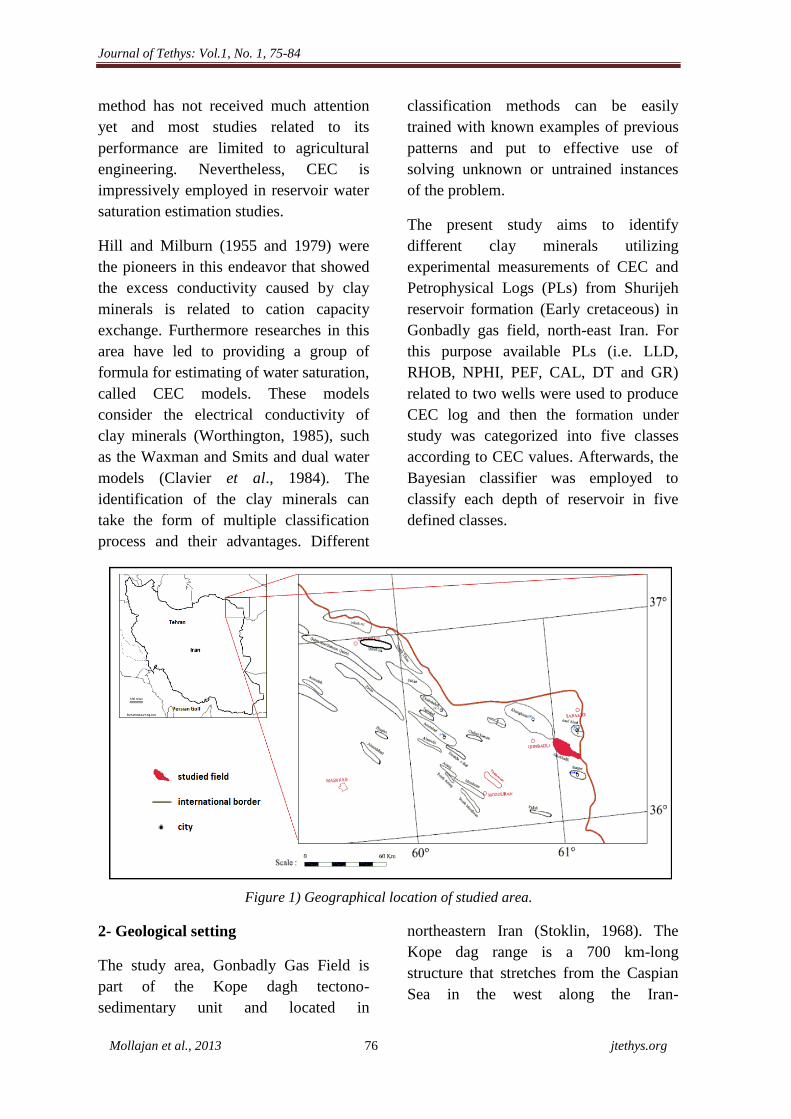
Figure 1) Geographical location of studied area.

2- Geological setting

The study area, Gonbadly Gas Field is

part of the Kope dagh tectono-

sedimentary unit and located in

northeastern Iran (Stoklin, 1968). The

Kope dag range is a 700 km-long

structure that stretches from the Caspian

Sea in the west along the Iran-



Turkmenistan border to Afghanistan in

the east (Fig. 1).

It forms the Iranian part of Alpine-

Himalayan mountain belt and consists of

a thick Tertiary-Mesozoic sedimentary

sequence, deposited in a deep and narrow

through. The whole complex was folded

in young alpine Neogene-Quaterner

phases (Eftekharnejad et al., 1991).

Cretaceous stratigraphic sequence in

study area is summarized in Table 1 as

follow:

Table1. Cretaceous stratigraphic sequence.

Era Period Formations

Mes

ozo

ic

Cre

tace

ou

s

Upper

Kalat

Nayzar

Abtalkh

Abderaz

Lower

Atamir

Sanganeh

Sarcheshmeh

Tirgan

Shurijeh

Shurijeh Formation as main reservoir in

Gonbadly gas field consists of red

continental sediments (sandstone,

siltstone and claystone). This formation

can be divided into 3 parts:

1- The upper part consist of red brown

to chocolate brown and white gray to

blue gray c coarse to medium grained

sandstone and siltstone alternating

with thin beds of red brown and

green grey partly gypsiferous, silty

clay to claystone.

2- The middle part of this formation is

composed of red brown and grey to

white grey hard quartzitic sandstone

interbeded with thin layers of reddish

brown siltstone and silty clay stone.

3- The lower part of this formation

consists of red brown to chocolate

brown gypsiferous claystone

alternating with thin beds of red

brown to chocolate brown and green

grey very fine grained partly

glauconitic sandstone and white hard

anhydrite.

The Shurijeh Formation is barren of

fossils but this formation should be of

Neocomian.

3- Data Set

3.1- Petrophysical Logs (PLs)

Data related to two wells of the Gonbadly

gas field have been used. The

petrophysical interpretation was made on

input: NPHI, RHOB, GR, DT, CAL,

LLD, and PEF for Shurijeh Formation.

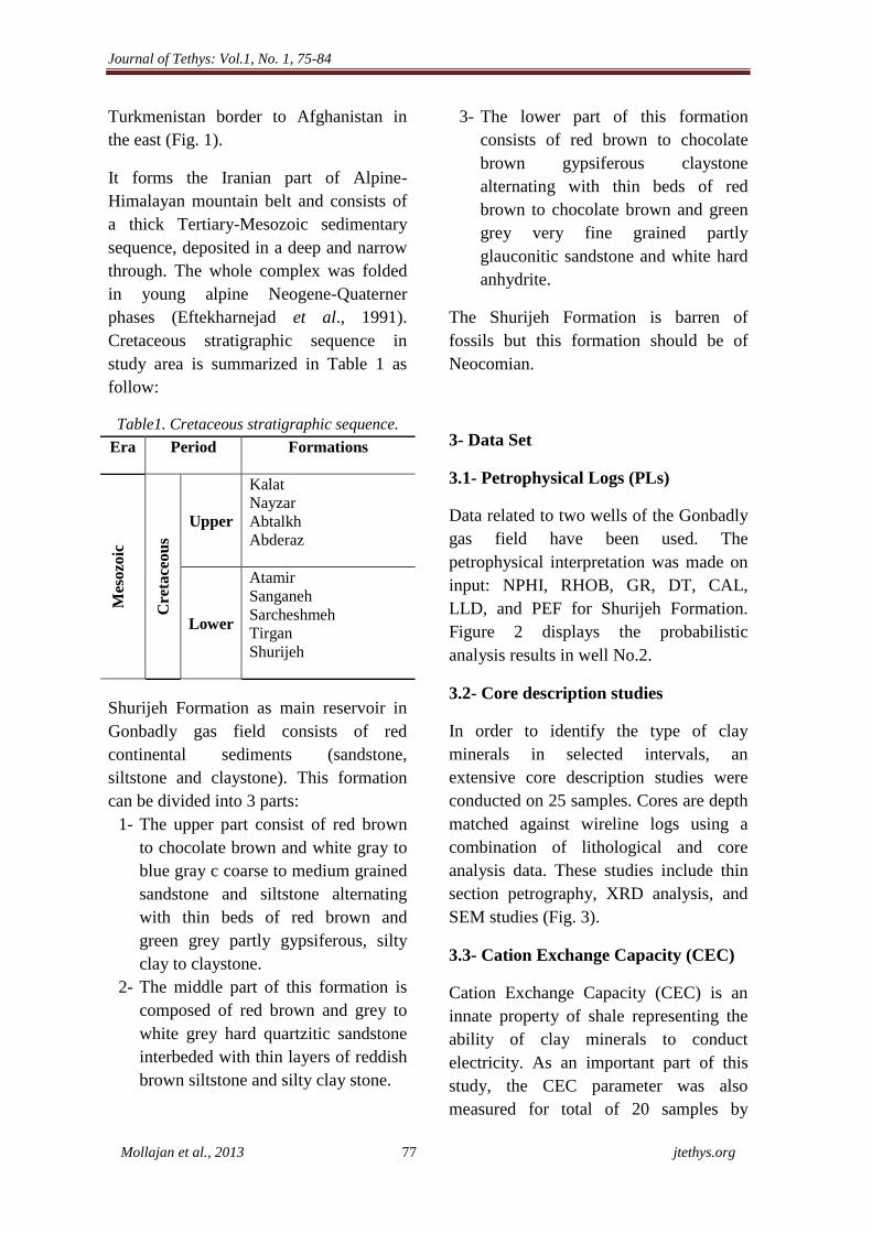
Figure 2 displays the probabilistic

analysis results in well No.2.

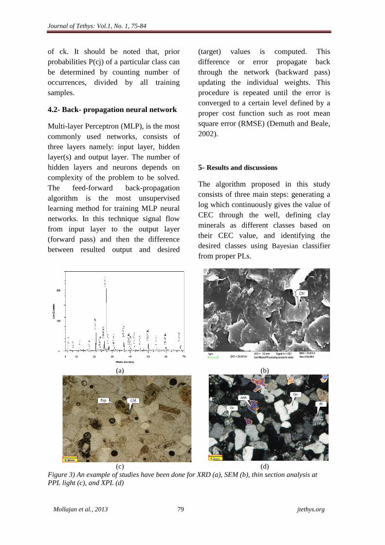
3.2- Core description studies

In order to identify the type of clay

minerals in selected intervals, an

extensive core description studies were

conducted on 25 samples. Cores are depth

matched against wireline logs using a

combination of lithological and core

analysis data. These studies include thin

section petrography, XRD analysis, and

SEM studies (Fig. 3).

3.3- Cation Exchange Capacity (CEC)

Cation Exchange Capacity (CEC) is an

innate property of shale representing the

ability of clay minerals to conduct

electricity. As an important part of this

study, the CEC parameter was also

measured for total of 20 samples by



bower method in laboratory (Richards,

1954).

4- Methodology

4.1- Bayesian classifier

The Bayesian classifier, developed based

on Bayes’ theorem is an effective

probabilistic algorithm, assigns the most

likely class to a given data. This classifier

uses the complete probability distribution

functions of the input features, and

assumes that all the Probability Density

Functions (PDFs) are known. In practice,

they should be estimated from the training

data. Bayes' formula allows us to express

the probability of a particular class given

an observed x as following (Duda and

Hart, 1973; Theodoridis and

Koutroumbas, 2003):

Eq.1 ( | )

( | )

Where x denotes the univariate or

multivariate input that could be well log

parameters (e.g. Vp or gamma ray). Let

cj, with j =l,...,N, indicates the N different

states or classes. P(x,cj) expresses the

joint probability of x and c and P(cj) is the

“prior probability” of a particular class

before having observed any x. P(cj│x)

known as “posterior probability”,

estimated from the training data or a

combination of training and forward

models (Duda and Hart, 1973).

Figure 2) Bulk mineralogy and PLs in well No. 2 for depth interval 3320 (m) to 3380 (m).

In Eq. (1), P(x) is probability of

belongings of each test data to each

possible class is calculated as follow

(Duda and Hart, 1973):

∑ ( | )

Eq.2

Based on this method, if P(ck│x) >

P(cj│x) for all j≠ k, x will assign to class



of ck. It should be noted that, prior

probabilities P(cj) of a particular class can

be determined by counting number of

occurrences, divided by all training

samples.

4.2- Back- propagation neural network

Multi-layer Perceptron (MLP), is the most

commonly used networks, consists of

three layers namely: input layer, hidden

layer(s) and output layer. The number of

hidden layers and neurons depends on

complexity of the problem to be solved.

The feed-forward back-propagation

algorithm is the most unsupervised

learning method for training MLP neural

networks. In this technique signal flow

from input layer to the output layer

(forward pass) and then the difference

between resulted output and desired

(target) values is computed. This

difference or error propagate back

through the network (backward pass)

updating the individual weights. This

procedure is repeated until the error is

converged to a certain level defined by a

proper cost function such as root mean

square error (RMSE) (Demuth and Beale,

2002).

5- Results and discussions

The algorithm proposed in this study

consists of three main steps: generating a

log which continuously gives the value of

CEC through the well, defining clay

minerals as different classes based on

their CEC value, and identifying the

desired classes using Bayesian classifier

from proper PLs.

(a) (b)

(c) (d)

Figure 3) An example of studies have been done for XRD (a), SEM (b), thin section analysis at

PPL light (c), and XPL (d)



In the following sections, the above

mentioned steps are described.

5.1- Predicting CEC log

The CEC log was predicted by a three-

layer MLP neural network on input logs:

LLD, RHOB, NPHI, PEF, CAL, DT, GR

and the CEC values measured from core

analysis as output. To build the ANN

predictor in most prediction problems, the

dataset must be divided into two parts: the

training set with 70% of the data points

and testing data with the remaining 30%.

However, the number of CEC measured

from core analysis in our study was low

(20 data), and information might have

been lost by dividing the dataset.

Therefore, the Leave-One-Out (LOO)

cross validation method as most useful

method was used to overcome this

problem. Through this method, 19 data

point were used for training and the

remaining one was used to validate the

ANN predictor.

A Lenvenberg-Marquardt training method

was used to optimize the weights. Table 2

displays the results of this stage.

Table 2) ANN CEC predictor model description

RMSE Number of neurons Function Model

3.97 7-10-1 TANSIG – LOGSIG – PURELINE CEC predictor

The result of selected ANN model for

CEC prediction is shown in Figure 4.

5.2- Applying cut offs

To consider the performance of the

algorithm proposed in this study, the

formation under study was divided into

five classes based on CEC values.

With respect to the range of the obtained

CEC log (between 0 and 135), four cut

offs were implemented by the use of the

standard CEC values. The class in which

the CEC value is below the limit of 3 was

considered as clean zone with a low

amount of Vsh. The applied cut offs are

shown in Table 3.

Table 3) The applied cut offs.

Defined class Applied cut off on CEC

value

Clean zone below the limit of 3

Kaolinite between the limits of 3

and 15

Illite or Chlorite between the limits of 15

and 40

Halloysite -

4H2O

between the limits of 40

and 70

Montmorillonite above the limit of 70

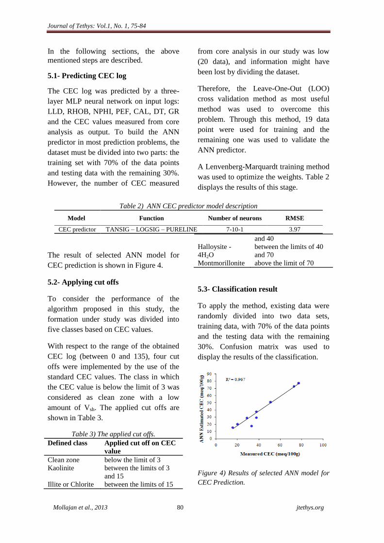
5.3- Classification result

To apply the method, existing data were

randomly divided into two data sets,

training data, with 70% of the data points

and the testing data with the remaining

30%. Confusion matrix was used to

display the results of the classification.

Figure 4) Results of selected ANN model for

CEC Prediction.



Confusion matrix is a squared matrix (5×5

in this study), whose rows and columns

represent decided and actual classes,

respectively.

The trace of this matrix indicates the total

accuracy of the method. The

Classification Correctness Rate (CCR)

was also calculated as an index by

dividing trace of confusion matrix by

number of classes. Classification was

performed in two stages:

a) At the first attempt, capability of

Bayesian classifier in identifying different

classes was examined in each individual

well separately (single well analysis).

b) At the second attempt, the

generalization capability of the method

was investigated, where input data from

one of the wells were used as train data to

identify the classes in the remaining well

(multi-well analysis).

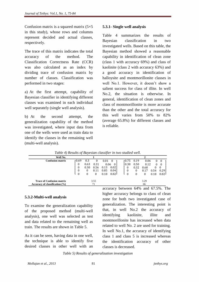
5.3.1- Single well analysis

Table 4 summarizes the results of

Bayesian classification in two

investigated wells. Based on this table, the

Bayesian method showed a reasonable

capability in identification of clean zone

(class 1 with accuracy 69%) and class of

kaolinite (class 2 with accuracy 63%) and

a good accuracy in identification of

halloysite and montmorillonite classes in

well No.1. However, it doesn’t show a

salient success for class of illite. In well

No.2, the situation is otherwise. In

general, identification of clean zones and

class of montmorillonite is more accurate

than the other and the total accuracy for

this well varies from 50% to 82%

(average 65.8%) for different classes and

is reliable.

Table 4) Results of Bayesian classifier in two studied well.

Well No. 1 2

Confusion matrix

[

]

[

]

Trace of Confusion matrix 3.55 3.29

Accuracy of classification (%) 71 66

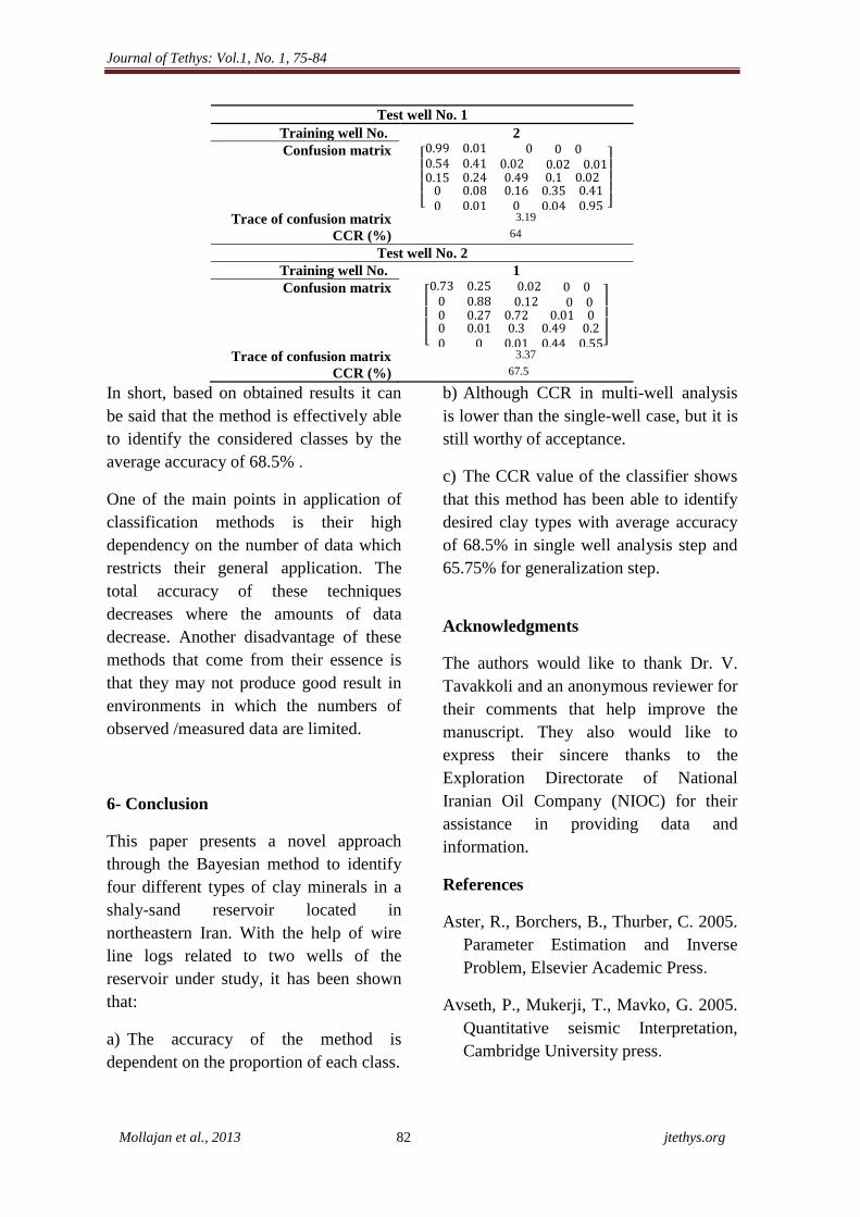
5.3.2-Multi-well analysis

To examine the generalization capability

of the proposed method (multi-well

analysis), one well was selected as test

and data related to the remaining well as

train. The results are shown in Table 5.

As it can be seen, having data in one well,

the technique is able to identify five

desired classes in other well with an

accuracy between 64% and 67.5%. The

higher accuracy belongs to class of clean

zone for both two investigated case of

generalization. The interesting point is

that, in well No.2 the accuracy of

identifying kaolinite, illite and

montmorillonite has increased when data

related to well No. 2 are used for training.

In well No.1, the accuracy of identifying

class 1 and class 5 is increased whereas

the identification accuracy of other

classes is decreased.

Table 5) Results of generalization investigation



Test well No. 1

Training well No. 2

Confusion matrix

[

]

Trace of confusion matrix 3.19

CCR (%) 64

Test well No. 2

Training well No. 1

Confusion matrix

[

]

Trace of confusion matrix 3.37

CCR (%) 67.5

In short, based on obtained results it can

be said that the method is effectively able

to identify the considered classes by the

average accuracy of 68.5% .

One of the main points in application of

classification methods is their high

dependency on the number of data which

restricts their general application. The

total accuracy of these techniques

decreases where the amounts of data

decrease. Another disadvantage of these

methods that come from their essence is

that they may not produce good result in

environments in which the numbers of

observed /measured data are limited.

6- Conclusion

This paper presents a novel approach

through the Bayesian method to identify

four different types of clay minerals in a

shaly-sand reservoir located in

northeastern Iran. With the help of wire

line logs related to two wells of the

reservoir under study, it has been shown

that:

a) The accuracy of the method is

dependent on the proportion of each class.

b) Although CCR in multi-well analysis

is lower than the single-well case, but it is

still worthy of acceptance.

c) The CCR value of the classifier shows

that this method has been able to identify

desired clay types with average accuracy

of 68.5% in single well analysis step and

65.75% for generalization step.

Acknowledgments

The authors would like to thank Dr. V.

Tavakkoli and an anonymous reviewer for

their comments that help improve the

manuscript. They also would like to

express their sincere thanks to the

Exploration Directorate of National

Iranian Oil Company (NIOC) for their

assistance in providing data and

information.

References

Aster, R., Borchers, B., Thurber, C. 2005.

Parameter Estimation and Inverse

Problem, Elsevier Academic Press.

Avseth, P., Mukerji, T., Mavko, G. 2005.

Quantitative seismic Interpretation,

Cambridge University press.



Batzle, M., Wang, Z. 1992. Seismic

properties of pore fluids. Geophysics:

57, 1396–1408.

Clavier, C., Coates, G., Dumanoir, J.

1984. Theoretical and experimental

bases for the dual water model for

interpretation of shaly sands. Society

of Petroleum Engineers Journal: 24,

153–168.

Demuth, H., Beale, M. 2002. Neural

network toolbox for use with

MATLAB, User’s guide,Version 4.

Dorothy, C. 1959. Ion exchange in clays

and other minerals, Geological Society

of America Bulletin: 70: 749–780.

Duda, R.O., Hart, P.E. 1973. Pattern

Classification and Scene Analysis,

New York: Wiley.

Eftekharnejad, J., Behroozi, A. 1991.

Geodynamic significance of recent

discoveries of ophiolites and late

Paleozoic rocks in NE Iran (including

Kope dagh). Abhandlungene der

geologischen Bundesanstalt: 38, 89–

100.

Hill, H.J., Shirley, O.J., Klein G.E. 1979.

Bound Water in Shaly Sands its

Relation to Qv and Other Formation

Properties, The Log Analyst.

Ipek, G. 2002. Log-derived Cation

Exchange Capacity of Shaly Sands,

PhD dissertation, Louisiana State

University.

Josh, M., Esteban, L., Delle Piane, C.,

Sarout, J., Dewhurst, D.N., Clennell,

M.B. 2012. Laboratory

characterisation of shale properties.

Journal of Petroleum Science and

Engineering: 88-89, 107-124.

Kurniawan, A. 2005. shaly sand

interpretation using CEC-dependent

petrophysical parameters," PhD

dissertation, Louisiana State

University.

Murphy, D.P., Chilingarian, G.V.,

Torabzadeh, S.J. 1996. Core analysis

and its application in reservoir

characterization. Developments in

Petroleum Science: 44, 105–153.

Richards, L.A. 1954. Diagnosis and

Improvement of saline and alkali soils,

united states department of agriculture,

Agriculture Handbook No. 60.

Serra, O. 1984. Fundamental of Well-Log

Interpretation- The Acquisition of

Logging Data. Elsevier science

publishers.

Stoklin, J. 1968. Strutural history and

tectonic of Iran. American

Assocciation of Petroleum Geologists

Bulletin: 52, 1229–1258.

Theodoridis S., Koutroumbos K. 2002.

Pattern Classification. 2nd

ed, San

Diego: Elsevier.

Worthington, P.F. 1985. The evolution of

shaly sand concepts in reservoir

evaluation. The Log Analyst: 26, 23–

40.

Zhang, D., Chun, C.H., Lin, C.X., Tong,

D.S., Yu, W.H. 2010, Synthesis of clay

minerals. Journal of Applied Clay

Science: 50, 1–11.

Received: 17 April 2013 / Accepted: 5 June

2013 / Published online: 8 June 2013



EDITOR-IN-CHIEF:

Dr. Vahid Ahadnejad:

Payame Noor University, Department of Geology.

PO BOX 13395-3697, Tehran, Iran.

E-Mail: [email protected]

EDITORIAL BOARD:

Dr. Jessica Kind:

ETH Zürich Institut für Geophysik, NO H11.3,

Sonneggstrasse 5, 8092 Zürich, Switzerland


Prof. David Lentz University of New Brunswick, Department of

Earth Sciences, Box 4400, 2 Bailey Drive

Fredericton, NB E3B 5A3, Canada


Dr. Anita Parbhakar-Fox

School of Earth Sciences, University of Tasmania,

Private Bag 126, Hobart 7001, Australia


Prof. Roberto Barbieri

Dipartimento di Scienze della Terra e

Geoambientali, Università di Bologna, Via

Zamboni 67 - 40126, Bologna, Italy


Dr. Anne-Sophie Bouvier

Faculty of Geosciences and Environment, Institut

des science de la Terre, Université de Lausanne,

Office: 4145.4, CH-1015 Lausann, Switzerland


Dr. Matthieu Angeli

The Faculty of Mathematics and Natural Sciences,

Department of Geosciences, University of Oslo

Postboks 1047 Blindern, 0316 OSLO, Norway


Dr. Miloš Gregor

Geological Institute of Dionys Stur, Mlynska

Dolina, Podjavorinskej 597/15 Dubnica nad

Vahom, 01841, Slovak Republic


Dr. Alexander K. Stewart

Department of Geology, St. Lawrence University,

Canton, NY, USA

E-mail: [email protected]

Dr. Cristina C. Bicalho

Environmental Geochemistry, Universidade

Federal Fluminense – UFF, Niteroi-RJ, Brazil

E-mail: [email protected]

Dr. Lenka Findoráková

Institute of Geotechnics, Slovak Academy of

Sciences, Watsonova 45, 043 53 Košice, Slovak

Republic


Dr. Mohamed Omran M. Khalifa

Geology Department, Faculty of Science, South

Valley, Qena, 83523, Egypt


Prof. A. K. Sinha

D.Sc. (Moscow), FGS (London). B 602,

VigyanVihar, Sector 56, GURGAON 122011,

NCR DELHI, Haryana


mailto:[email protected]












Documents

A Bayesian approach to identify clay minerals from ...jtethys.org/wp-content/uploads/2013/10/Mollajan_et_al_2013.pdf · A Bayesian approach to identify clay minerals from petrophysical