Embed Size (px)
Citation preview
A Bayesian Approach to Map-AidedVehicle Positioning
Examensarbete utfort i Reglerteknikvid Tekniska Hogskolan i Linkoping
av
Peter Hall
Reg nr: LiTH-ISY-EX-3102

A Bayesian Approach to Map-AidedVehicle Positioning
Examensarbete utfort i Reglerteknikvid Tekniska Hogskolan i Linkoping
av
Peter Hall
Reg nr: LiTH-ISY-EX-3102
Supervisor: Urban ForssellPer-Johan Nordlund
Examiner: Fredrik Gunnarsson
Linkoping, 22nd January 2001.

Abstract i
Abstract
There is an increasing market for navigation systems and services asso-ciated with positioning in today’s automotive informatics and telematics.Contemporary positioning systems have some drawbacks, mainly relatedto expensive hardware requirements and that the reliability occasionally israther low. Therefore it is interesting to develop positioning techniques thatdo not share these disadvantages.
In this thesis the approach is to use low cost sensor equipment and digitallystored map information to produce a high performance vehicle positioningmodule. To be able to do this, the problem has been formulated as a non-linear estimation problem, to which Bayesian estimation has been applied.Two approximate solutions have been evaluated: A grid based method,referred to as the point-mass filter, and a sequential Monte Carlo method.
Simulations show that it is possible to obtain independent position estimateswith an accuracy comparable to gps (Global Positioning System), using thistechnique. A positioning system based on the suggested method can thusbe used stand-alone or as a complement to existing systems.
Key Words: Positioning, Vehicle Navigation, Nonlinear Filtering, BayesianEstimation, Monte Carlo Methods.

ii Abstract
Abstract iii
Acknowledgments
First of all I would like to thank my supervisors, Urban Forssell and Per-Johan Nordlund for their support and encouragement during my work onthis thesis. I also would like to thank my examiner Fredrik Gunnarson andProfessor Fredrik Gustafsson for valuable comments and Ulf Gustafssonfor reviewing this thesis. Furthermore, I am grateful to Stefan Ahlqvist,Martin Enqvist and Erik Wernholt for interesting discussions and technicalassistance. Finally I would like to thank Anders Stenman for helping me outwith LATEX and the rest of the staff at NIRA Automotive AB in Linkopingfor making my time there enjoyable.
Linkoping, Januari 2001Peter Hall

iv Abstract
Notation v
Notation
Notational conventions for mathematical symbols and operators and somecommon abbreviations are presented in this section.
Symbols
p(x) Probability density function (pdf) for the stochastic variable x.p(x, y) Joint pdf for x and y.p(x|y) Conditional pdf for x given a certain value of y.x The estimate of a stochastic variable x.Rn The n-dimensional Euclidian space.Ts Sample period, i.e. if data is sampled with fs Hz,
then Ts = 1fs
.
Operators and Functions
E(x) Expectation of a stochastic variable x.‖u‖2 The 2-norm of a vector u.trA The trace of a matrix A.
Abbreviations
ABS Anti-Lock Braking System.CAN Controller Area Network.CEP Circular Error Probable.DGPS Differential GPS.EKF Extended Kalman Filter.GLONASS GLObal NAvigation Satellite System.GPS Global Positioning System.GUI Graphical User Interface.INS Inertial Navigation System.

vi Notation
MAP Maximum A Posteriori.MC Monte Carlo.MMS Minimum Mean Square.PDF Probability Density FunctionPMF Point-Mass Filter.RMSE Root Mean Square Error.SIR Sampling Importance Resampling.SIS Sequential Importance Sampling.
Contents vii
Contents
1 Introduction 11.1 Background . . . . . . . . . . . . . . . . . . . . . . . . . . . . 11.2 NIRA Automotive AB . . . . . . . . . . . . . . . . . . . . . . 21.3 Problem Specification . . . . . . . . . . . . . . . . . . . . . . 31.4 Objectives . . . . . . . . . . . . . . . . . . . . . . . . . . . . . 31.5 Thesis Outline . . . . . . . . . . . . . . . . . . . . . . . . . . 4
2 Positioning Technologies 52.1 Coordinate Systems . . . . . . . . . . . . . . . . . . . . . . . 52.2 Dead Reckoning . . . . . . . . . . . . . . . . . . . . . . . . . . 62.3 Relative Sensors . . . . . . . . . . . . . . . . . . . . . . . . . 6
2.3.1 Gyroscopes . . . . . . . . . . . . . . . . . . . . . . . . 62.3.2 Accelerometers . . . . . . . . . . . . . . . . . . . . . . 72.3.3 Wheel Speed Sensors . . . . . . . . . . . . . . . . . . . 7
2.4 Additional Sources of Error . . . . . . . . . . . . . . . . . . . 82.5 Absolute Sensors . . . . . . . . . . . . . . . . . . . . . . . . . 8
2.5.1 Satellite-based Navigation Systems . . . . . . . . . . . 82.5.2 Magnetic Compasses . . . . . . . . . . . . . . . . . . . 92.5.3 Positioning in Cellular Radio Systems . . . . . . . . . 10
2.6 Sensor Fusion . . . . . . . . . . . . . . . . . . . . . . . . . . . 102.7 Map Matching . . . . . . . . . . . . . . . . . . . . . . . . . . 11
2.7.1 Semi-Deterministic Algorithms . . . . . . . . . . . . . 112.7.2 Probabilistic Algorithms . . . . . . . . . . . . . . . . . 11
2.8 Map Representation . . . . . . . . . . . . . . . . . . . . . . . 12
3 Map-Aided Positioning 133.1 Problem Specification . . . . . . . . . . . . . . . . . . . . . . 133.2 Limitations . . . . . . . . . . . . . . . . . . . . . . . . . . . . 143.3 Methods . . . . . . . . . . . . . . . . . . . . . . . . . . . . . . 14
4 Bayesian Estimation 154.1 Basics . . . . . . . . . . . . . . . . . . . . . . . . . . . . . . . 154.2 Recursive Estimation . . . . . . . . . . . . . . . . . . . . . . . 154.3 Grid Based Methods . . . . . . . . . . . . . . . . . . . . . . . 17
4.3.1 The Point-Mass Filter . . . . . . . . . . . . . . . . . . 174.3.2 Grid Adaptation . . . . . . . . . . . . . . . . . . . . . 19
4.4 Monte Carlo Methods . . . . . . . . . . . . . . . . . . . . . . 204.4.1 Monte Carlo Integration . . . . . . . . . . . . . . . . . 20

viii List of Figures
4.4.2 Sequential Monte Carlo Methods . . . . . . . . . . . . 214.4.3 Particle Filters . . . . . . . . . . . . . . . . . . . . . . 22
5 Vehicle Positioning 255.1 Implementation . . . . . . . . . . . . . . . . . . . . . . . . . . 25
5.1.1 The Point-Mass Filter . . . . . . . . . . . . . . . . . . 255.1.2 The Particle Filter . . . . . . . . . . . . . . . . . . . . 26
5.2 Performance Evaluation . . . . . . . . . . . . . . . . . . . . . 265.2.1 Measurement Data Acquisition . . . . . . . . . . . . . 265.2.2 Particle Clustering . . . . . . . . . . . . . . . . . . . . 285.2.3 Improvements of the Particle Filter Implementation . 305.2.4 Evaluation Using Real Measurements . . . . . . . . . 315.2.5 Monte Carlo Simulations . . . . . . . . . . . . . . . . 35
5.3 Discussion . . . . . . . . . . . . . . . . . . . . . . . . . . . . . 38
6 Heading Angle Estimation 396.1 Model Extension . . . . . . . . . . . . . . . . . . . . . . . . . 396.2 Implementation . . . . . . . . . . . . . . . . . . . . . . . . . . 406.3 Performance Evaluation . . . . . . . . . . . . . . . . . . . . . 40
6.3.1 Monte Carlo Simulations . . . . . . . . . . . . . . . . 416.3.2 Robustness . . . . . . . . . . . . . . . . . . . . . . . . 41
6.4 Discussion . . . . . . . . . . . . . . . . . . . . . . . . . . . . . 44
7 Conclusions 47
8 Future Work 47
References 48
Appendix A: Bayes’ Rule 50
Appendix B: Bayesian Solution to the 3D Problem 51
List of Figures
2.1 Coordinate systems . . . . . . . . . . . . . . . . . . . . . . . . 54.1 The point-mass representation . . . . . . . . . . . . . . . . . 194.2 Importance weighting and resampling procedure of the par-
ticle filter . . . . . . . . . . . . . . . . . . . . . . . . . . . . . 235.1 Convergence problems with the particle filter . . . . . . . . . 27
List of Figures ix
5.2 The test drives used in the simulations. . . . . . . . . . . . . 285.3 An example of particle clustering . . . . . . . . . . . . . . . . 295.4 Simulation results of the pmf using data from sequence S1. . 325.5 Simulation results of the particle filter using data from se-
quence S1. . . . . . . . . . . . . . . . . . . . . . . . . . . . . . 325.6 The prior editing ratio for the simulation in Figure 5.5. . . . 335.7 Simulation results of the particle filter when the track is lost. 345.8 rmse for the particle filter based on 100 Monte Carlo simu-
lations . . . . . . . . . . . . . . . . . . . . . . . . . . . . . . . 365.9 Monte Carlo simulations of two different driving scenarios
using the two-dimensional particle filter . . . . . . . . . . . . 376.1 Monte Carlo simulations of two different driving scenarios
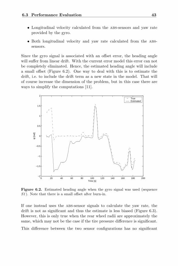
using the two-dimensional particle filter . . . . . . . . . . . . 426.2 Estimated heading angle when the gyro signal was used . . . 436.3 Estimated heading angle when the wheel-speed signals were
used to compute the yaw rate . . . . . . . . . . . . . . . . . . 44

x List of Figures
1 Introduction 1
1 Introduction
1.1 Background
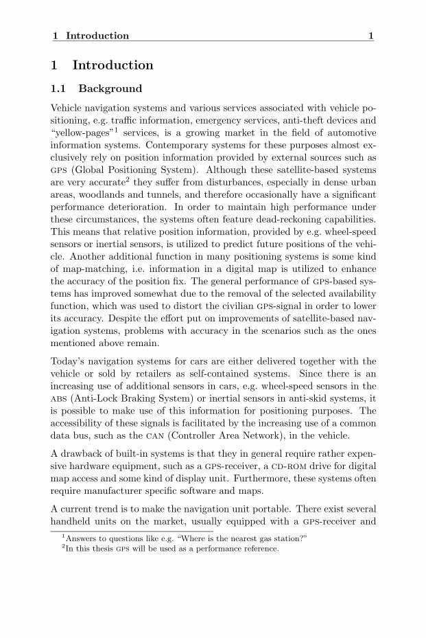
Vehicle navigation systems and various services associated with vehicle po-sitioning, e.g. traffic information, emergency services, anti-theft devices and“yellow-pages”1 services, is a growing market in the field of automotiveinformation systems. Contemporary systems for these purposes almost ex-clusively rely on position information provided by external sources such asgps (Global Positioning System). Although these satellite-based systemsare very accurate2 they suffer from disturbances, especially in dense urbanareas, woodlands and tunnels, and therefore occasionally have a significantperformance deterioration. In order to maintain high performance underthese circumstances, the systems often feature dead-reckoning capabilities.This means that relative position information, provided by e.g. wheel-speedsensors or inertial sensors, is utilized to predict future positions of the vehi-cle. Another additional function in many positioning systems is some kindof map-matching, i.e. information in a digital map is utilized to enhancethe accuracy of the position fix. The general performance of gps-based sys-tems has improved somewhat due to the removal of the selected availabilityfunction, which was used to distort the civilian gps-signal in order to lowerits accuracy. Despite the effort put on improvements of satellite-based nav-igation systems, problems with accuracy in the scenarios such as the onesmentioned above remain.
Today’s navigation systems for cars are either delivered together with thevehicle or sold by retailers as self-contained systems. Since there is anincreasing use of additional sensors in cars, e.g. wheel-speed sensors in theabs (Anti-Lock Braking System) or inertial sensors in anti-skid systems, itis possible to make use of this information for positioning purposes. Theaccessibility of these signals is facilitated by the increasing use of a commondata bus, such as the can (Controller Area Network), in the vehicle.
A drawback of built-in systems is that they in general require rather expen-sive hardware equipment, such as a gps-receiver, a cd-rom drive for digitalmap access and some kind of display unit. Furthermore, these systems oftenrequire manufacturer specific software and maps.
A current trend is to make the navigation unit portable. There exist severalhandheld units on the market, usually equipped with a gps-receiver and
1Answers to questions like e.g. “Where is the nearest gas station?”2In this thesis gps will be used as a performance reference.
2 1 Introduction
maps stored in an internal memory. In general these systems are not suitedfor vehicle navigation and are basically handheld gps-receivers with mapdisplaying capabilities.
In order to reduce the price of the complete navigation package, several dif-ferent solutions are represented on the market. For example, the cd-romunit can be replaced by downloadable maps, route guidance calculationscan be delegated to a call center via a cellular connection etc. In the caseof handheld navigators, there exist systems based on personal digital as-sistants (pda’s), which provide the fundamental computing and displayinghardware. These can be attached to a compact gps-receiver and furnishedwith navigation software.
The backbone of a vehicle navigation system is a high precision positioningmodule, available at a low cost. In other words, to continuously providethe driver with reliable information about the position of the vehicle, with-out requiring expensive additional hardware. It is thus of great interestto develop alternative positioning techniques that does not have the sameweaknesses as the satellite-based ones, and that provides state-of-the-artperformance at a low cost. The latter is interesting for car manufacturersas well as for the car owners.
1.2 NIRA Automotive AB
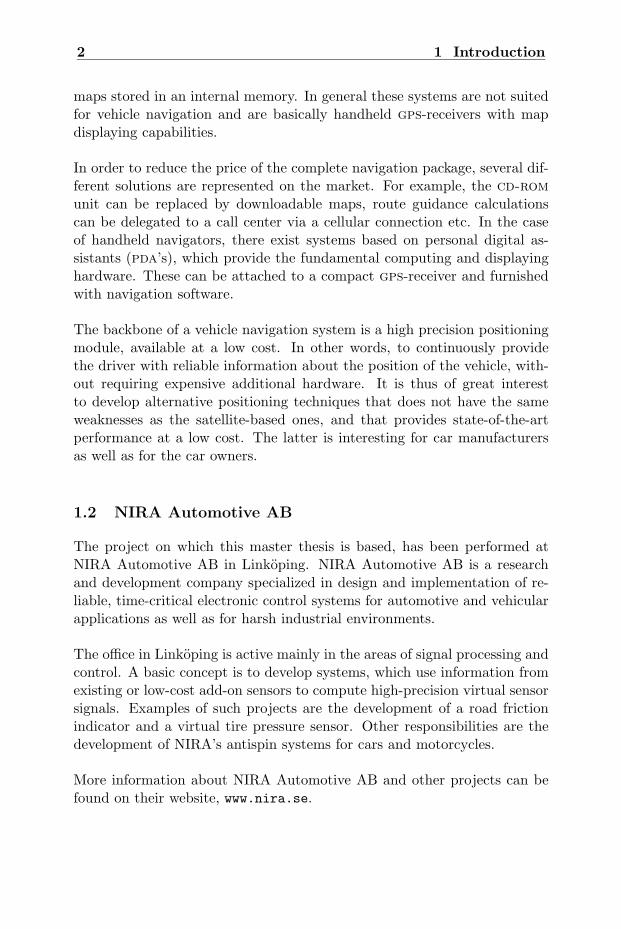
The project on which this master thesis is based, has been performed atNIRA Automotive AB in Linkoping. NIRA Automotive AB is a researchand development company specialized in design and implementation of re-liable, time-critical electronic control systems for automotive and vehicularapplications as well as for harsh industrial environments.
The office in Linkoping is active mainly in the areas of signal processing andcontrol. A basic concept is to develop systems, which use information fromexisting or low-cost add-on sensors to compute high-precision virtual sensorsignals. Examples of such projects are the development of a road frictionindicator and a virtual tire pressure sensor. Other responsibilities are thedevelopment of NIRA’s antispin systems for cars and motorcycles.
More information about NIRA Automotive AB and other projects can befound on their website, www.nira.se.
1.3 Problem Specification 3
1.3 Problem Specification
A fundamental component in a navigation system is a reliable and accu-rate positioning module. Positioning is the determination of the global (orabsolute) coordinates of the vehicle, i.e. to specify the vehicle’s positionin a known reference frame. One example of such a reference frame is ageographical map.
In order to present correct information about the vehicle location to thedriver, the position provided from the positioning module is usually matchedto a digital map. The basic idea of map matching is to compare the outputfrom the positioning module, i.e. the trajectory of the vehicle, against theshape of nearby roads and choose the closest match.
The idea in this thesis is to fuse positioning and map matching into a map-aided positioning algorithm, which does not require external absolute po-sition fixes, e.g. provided by gps. This is achieved by integrating signalsfrom relative sensors (e.g. wheel speed sensors, accelerometers, gyroscopes)with the information contained in a digital map. As can be imagined, thisis a very complex and nonlinear filtering problem, to which Bayesian esti-mation methods are applied. This approach is inspired by the Ph.D. workof Bergman [1]. The ideas on map-aided positioning, as defined here, arepatent pending.
The problem has been divided into two parts:
• To estimate the absolute position when the absolute heading is known.
• To extend the model and estimate the absolute heading angle as well.
1.4 Objectives
The purpose of this thesis is to investigate the possibilities of applyingBayesian estimation techniques to the problem described in the previoussection.
To achieve this, the following issues have to be considered:
• A mathematical model suitable for the vehicle positioning problem hasto be developed. This includes how to model the map information.
• A simulation environment, where the studied algorithms are to beimplemented, has to be developed.
• The positioning filters should be evaluated using real measurementdata, collected during authentic driving scenarios.
4 1 Introduction
1.5 Thesis Outline
In Section 2 a review of position technologies as well as common sourcesof error and an introduction to map-matching techniques is presented as abackground to the problems discussed in this report. Section 3 describesthe first part of the actual problem, the estimation of the absolute positionwhen the heading angle is known. Furthermore an introduction to Bayesianestimation methods is given in Section 4, while Section 5 treats the applica-tion of these methods to the problem in Section 3. In Section 6 the problemis extended to include estimation of the heading angle. Finally, the reportis concluded in Section 7, while future work is discussed in Section 8.
2 Positioning Technologies 5
2 Positioning Technologies
There are mainly three positioning technologies used in vehicle navigation:stand-alone (e.g. dead reckoning), satellite-based (e.g. gps), and terrestrialradio based. This section will give a brief review of these areas as wellas an introduction to the basic ideas of map matching. A more thoroughintroduction to vehicle positioning and navigation systems can be found in[12].
2.1 Coordinate Systems
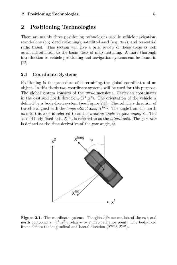
Positioning is the procedure of determining the global coordinates of anobject. In this thesis two coordinate systems will be used for this purpose.The global system consists of the two-dimensional Cartesian coordinatesin the east and north direction, (x1, x2). The orientation of the vehicle isdefined by a body-fixed system (see Figure 2.1). The vehicle’s direction oftravel is aligned with the longitudinal axis, X long. The angle from the northaxis to this axis is referred to as the heading angle or yaw angle, ψ. Thesecond body-fixed axis, X lat, is referred to as the lateral axis. The yaw rateis defined as the time derivative of the yaw angle, ψ.
Figure 2.1. The coordinate systems. The global frame consists of the east andnorth components, (x1, x2), relative to a map reference point. The body-fixedframe defines the longitudinal and lateral direction (X long, X lat).
6 2 Positioning Technologies
2.2 Dead Reckoning
Dead reckoning is a primitive positioning technique that involves integrationof relative movements with respect to time starting from a known referencepoint. The idea is that, if the initial position is known, it is possible to cal-culate the vehicle position at any instance by measuring the displacementsin distance and direction.
A common dead-reckoning system is the Inertial Navigation System (ins)which uses inertial sensors like accelerometers and gyroscopes to measurethe magnitude of the acceleration and the angular rates (e.g. yaw rate) ofthe vehicle.
2.3 Relative Sensors
A generic term for sensors that measure changes in position or heading,i.e. movements relative an absolute position, is relative sensors [12]. Apartfrom the inertial sensors there exist several other relative automotive sen-sors, e.g. transmission pickups, which measure the angular position of thetransmission shaft, or wheel speed sensors (such as the ones used in theAnti-Lock Braking System, abs).
Important characteristics of dead reckoning using relative sensors are thatif the initial position is unknown, the information can not be used for ab-solute positioning purposes. Another feature is that measurement errorsare accumulated due to the integration operation and after some time thedeviation from the actual trajectory can be considerably large.
2.3.1 Gyroscopes
A rate-sensing gyroscope measures the angular rate using either mechanical,optical, pneumatic or vibrational devices. The performance of the gyroscopeis characterized by several factors. For example the measurements usuallysuffer from scale factor errors, drift (offset error) and measurement noise.The output from a gyroscope can be modeled as
ψgyro(t) = (1 + α)ψ(t) + δgyro + C · t + e(t), (2.1)
where α is a scale factor error, δgyro is an offset term, C is a linear driftterm and e is measurement noise.
2.3 Relative Sensors 7
2.3.2 Accelerometers
An accelerometer can be used to measure the acceleration in a given direc-tion, e.g. along the coordinate axis of a body-fixed frame. In similarity withthe gyroscope, the following model can be used for the accelerometer signal
aacc(t) = (1 + α)a(t) + δacc + C · t + e(t). (2.2)
2.3.3 Wheel Speed Sensors
A wheel speed sensor consists of a toothed ferrous wheel, mounted on thewheel axle, and some kind of sensing element (e.g. a variable reluctance ora Hall-effect sensor [12]). The sensor measures the rotational velocity ofthe wheel, ωw. Assuming that the nominal radius of the wheel is rn andthat the actual radius has some offset, δw, the wheel speed of a free-rolling(undriven) wheel can be modeled as
vw(t) = (rn + δw)ωw(t)︸ ︷︷ ︸circumferential velocity
+e(t), (2.3)
where the measurement noise is modeled as an additive term, e.
If the wheel is driven, or during braking, another error is introduced due tothe fact that the absolute velocity of the wheel, vw, does no longer coincidewith its circumferential velocity as assumed in (2.3). This error, whichplays an important role in automotive engineering, is called wheel slip andis usually defined as the relative difference [7]
s(t) =(rn + δw)ωw(t) − vw(t)
vw(t). (2.4)
Wheel speed sensors can be used to estimate the longitudinal velocity of thevehicle. Usually this is achieved by averaging the angular rates of either thefront or the rear wheel pairs and multiplying by a proper scale factor (e.g.the nominal wheel radius)
vlong(t) = rnωw ,right(t) + ωw ,left(t)
2. (2.5)
A yaw rate estimate can be obtained by calculating the difference in angularrate between the right and left rear wheels and dividing by the rear axlelength, lrear

8 2 Positioning Technologies
ψ(t) = rnωw ,right(t) − ωw ,left(t)
lrear. (2.6)
This technique to provide both longitudinal velocity and yaw rate infor-mation from a pair of wheel speed sensors is called differential odometry[12].
2.4 Additional Sources of Error
Apart from inaccuracy in the sensors there are some other sources of errorthat have to be considered. Some examples are the wheel radii offset and thewheel slip mentioned above. Another disturbance is the road inclination,which, if not compensated for, causes erroneous sensor signals and alsoconflicts with the implicit assumption that the vehicle is located on a flatmap.
Example 2.1. A longitudinal accelerometer measures the magnitude of theacceleration in the direction of travel. If the road has a slight inclination,α, the accelerometer will also measure a component of the gravitationalacceleration, g. If the other errors are assumed to be zero this yields
aacc(t) = a(t) + g sinα (2.7)
Even if the inclination is moderate this will give a significant deteriorationin a dead-reckoning system due to the accumulation of errors, described inSection 2.3.
2.5 Absolute Sensors
The opposite to a relative sensor is an absolute sensor, which measures theabsolute position (e.g. gps) or the absolute heading (e.g. magnetic com-passes).
2.5.1 Satellite-based Navigation Systems
There are two global satellite-based navigation systems available today, orig-inally developed for military purposes: gps, which is the U.S. alternativeand most commonly used in vehicle navigation systems, and the correspond-ing Russian system glonass. Some more expensive navigation systems use
2.5 Absolute Sensors 9
a combination of these systems in order to achieve higher performance. TheEuropean Space Agency (esa) is also planning for a third, all Europeansystem, which is to be operational from 2005 under current plans.
The Global Positioning System [12] (gps) is a satellite-based radio navi-gation system, that consists of 24 satellites arranged in six orbital planes,designed to provide worldwide coverage 24 hours per day. Each of the satel-lites carries a high precision atomic clock and broadcasts encoded messagesat regular and known time instants. Each message includes an identitynumber and the location of the satellite. A receiver on the ground decodesthe signal and uses the signal propagation time to calculate a pseudorange.To determine its position, the receiver needs to know the pseudoranges tothe satellites as well as their locations. If a position estimate in three di-mensions is desired this information should be available from at least fourunique satellites. Three satellites are required to solve the three unknownCartesian coordinates and the extra satellite handles the fact that the mea-sured pseudorange is not the actual range, due to receiver clock bias.
If a reference receiver with known position is used to calculate a differen-tial correction for each satellite, the accuracy of gps can be significantlyimproved. This idea is adopted in the differential gps (dgps), which usesa constellation of ground-based reference stations to provide the mobile re-ceivers with position fixes.
The position obtained from a gps receiver includes several error terms ofmore or less importance for the general performance of the system. Forexample there are range errors due to ionospheric and tropospheric delay,but such disturbances can usually be estimated using atmospheric models.Other errors that are involved are receiver noise, multipath propagation er-ror (i.e. when the signal is received with a time lag caused by reflections),and satellite orbit error. For vehicle navigation applications, gps receiverperformance under heavy foliage and in urban canyon areas is particularlyimportant. Overhead foliage may cause signal attenuation and high build-ings may block the satellite signals or cause multipath errors.
2.5.2 Magnetic Compasses
By absolute heading one usually refers to the orientation of the vehiclerelative to the north. This quantity can be determined by measuring theearth’s magnetic field, e.g. by using a magnetic compass. However, themagnetic north deviates from the true north and this difference is known
10 2 Positioning Technologies
as declination. To correct the deviation, which varies both with time andgeographical location, a declination table can be used.
The most commonly used type of magnetic compass is the electronic fluxgatecompass. Although electronic compasses have higher vibration durabilityand quicker response than conventional compasses, they still are quite sensi-tive to magnetic anomalies and noise. However, there exist several methodsof improving the performance, e.g. low-pass filtering and correction tables[12].
If a compass is used in a vehicle, the magnetic field of the vehicle itself willinterfere with the measurement. This error is often referred to as magneticdeviation, and its magnitude depends on the true heading of the vehicle.One way of compensating for magnetic deviation is to use a look-up tablecontaining correction information for any heading. Another way is to esti-mate the error dynamically, which is fairly simple since the measured fieldvector is the sum of the earth’s field vector and the field vector generatedby the vehicle.
2.5.3 Positioning in Cellular Radio Systems
An example of a terrestrial radio-based system used for positioning are cellu-lar radio systems. When distributing transmission power to handsets in thenearby area, the base stations in the network use rough position estimatesbased on measurements on the incoming signals. This information can beforwarded to the handset and used e.g. in a yellow-pages service or for nav-igation purposes. Contemporary systems provide estimates with very lowaccuracy, but future generations are expected to improve this considerably.An overview of various techniques can be found in [5].
2.6 Sensor Fusion
From the discussion in the previous sections, it is obvious that no singlesensor can provide completely accurate position information. Thus it isdesirable to have a multisensor configuration and merge the available infor-mation in order to increase the overall performance.
The idea of using several different sensors and extracting the combinedinformation from the observations is referred to as sensor fusion. There areseveral advantages with the fusing process, e.g. increased accuracy, increaseddegree of confidence or reduced ambiguity. This is of course valid only ifthe sensor models used describe the true properties of the physical sensors.
2.7 Map Matching 11
A common statistical approach to sensor fusion is to use Kalman filtering.A detailed description of this can be found in [9].
2.7 Map Matching
An important part of vehicle navigation is to present the current positionin a satisfactory fashion to the driver. Usually this involves displaying thevehicle location on a digital road map. To provide this kind of informa-tion, an accurate vehicle position obtained from the positioning module isrequired. However, since there are errors associated with the position es-timates, the actual position does not necessarily agree with the measuredposition. These errors are often of cumulative nature and thus the deviationis likely to increase with time.
To deal with this discrepancy some kind of map-matching algorithm is oftenemployed to correct the measured position so that it fits on the map. Ifproperly done, this will enhance the accuracy of the position estimate.
The basic idea of conventional map matching is to compare the outputfrom the positioning module, i.e. the trajectory of the vehicle, with theshape of nearby roads and choose the closest match. There exist both semi-deterministic and probabilistic map matching algorithms.
2.7.1 Semi-Deterministic Algorithms
Semi-deterministic map matching is based on the presumption that thevehicle is traveling on the road network. The matching procedure utilizesgeometric and topological information to correct the errors in the positionestimate. A very simple example of a semi-deterministic match is to snapthe position estimate to the nearest road in the network. However, this isonly feasible if the estimate and the network model is very accurate. Moresophisticated algorithms can be found in [2].
2.7.2 Probabilistic Algorithms
To improve the performance of map-matching algorithms some informationabout the accuracy of the position estimate should be incorporated withthe spatial information of the map. This idea is adopted in probabilisticmap-matching algorithms. Based on models of the sensor errors, confidenceregions can be defined for the estimate. If these regions are superimposed onthe road network it is possible to determine the most probable road segmentfrom which the estimate originates. A major enhancement of this method
12 2 Positioning Technologies
over the semi-deterministic method is that the vehicle does not necessarilyhave to be confined to the road. If no road segment candidate intersects theconfidence region the algorithm leaves the position unmatched, i.e. the fixprovided by the positioning module is not corrected.
For further discussions about conventional map-matching algorithms see[12], which also describes some alternative methods.
2.8 Map Representation
In order to implement a high performance positioning algorithm, whichrelies on map information, it is of vital importance that the representationof the map is efficient and accurate.
There are in general two major ways to represent map information in acomputer. One is to digitize the paper map using a scanner to produce araster encoded structure, which will more or less be an exact copy of theoriginal. Another way is to convert the information into a vector-encodedstructure. This procedure will extract only the most relevant features of themap resulting in a more efficient and flexible representation. In a navigationapplication the vector-encoded format is superior to the raster-encoded for-mat concerning the possibility to use mathematical models and calculationsas well as the lower memory requirements. Therefore this report will focuson the vector-encoded representation.
3 Map-Aided Positioning 13
3 Map-Aided Positioning
The basic idea in this thesis is to use the information in a digital maptogether with a standard dead-reckoning system to solve the vehicle po-sitioning problem. This is tackled from a statistical viewpoint using theconcept of sensor fusion. Since the approach is quite different from conven-tional map matching the term map-aided positioning is used here. In thefollowing sections, the problem will be formulated mathematically.
3.1 Problem Specification
Let xt denote the position of the vehicle and let ut denote the relative move-ment measured by relative sensors (such as gyroscopes and wheel sensors).If the drift in the relative sensors is modeled by random walk, the statetransition equation can be written as
xt+1 = xt + ut + vt, (3.1)
where vt is white noise with density function pv(·). To integrate map infor-mation in the model one can introduce measurements, denoted by yt. Therelation between these measurements and the vehicle position is modeled as
yt = h(xt) + et, (3.2)
where h(·) is some nonlinear function and et is white measurement noise withdensity function pe(·). The processes et and vt are statistically independent.A measurement of particular interest is the minimum Euclidean distancefrom an arbitrary point in the state space, to the road network. The functionh(·) thus represents the corresponding distance obtained from the map. LetΩR denote the road network then
h(xt) = minx∈ΩR
‖xt − x‖2. (3.3)
The equations (3.1) and (3.2) define a nonlinear recursive estimation prob-lem
xt+1 = xt + ut + vt
yt = h(xt) + et,(3.4)
to which Bayesian estimation theory will be applied in Section 4.2.
14 3 Map-Aided Positioning
3.2 Limitations
In the first study of the positioning problem only the absolute position ofthe vehicle is considered unknown. This means that the absolute headingof the vehicle is assumed to be known, perhaps from measurements by amagnetic fluxgate compass.
Another assumption is that the vehicle is always located on a road. Thisconstraint means that the measurement of the minimum distance from thevehicle to the road is simply zero plus some measurement noise (et). Theroad network, ΩR, defines a subspace to the state space, which here is R2.The spatial structure of the road network contains valuable information forpositioning.
3.3 Methods
The estimation problem will be studied from a Bayesian viewpoint [1] usingtwo methods to approximate the optimal analytical solution. In the nextsection a brief review of recursive Bayesian estimation is presented.
4 Bayesian Estimation 15
4 Bayesian Estimation
4.1 Basics
State space estimation is the procedure of gaining information about thestate of a system by observing some kind of related quantity. In a Bayesianframework the state as well as the measurement are treated as stochasticvectors. Let the likelihood of the measurement y, given the state x bedenoted by p(y|x). By considering the prior knowledge about the state,p(x), i.e. what is known before obtaining the measurement, the joint densityof the state and the observation
p(x, y) = p(y|x)p(x) (4.1)
defines a statistical model for the estimation problem. Applying Bayes’ rule(Appendix A) yields
p(x|y) =p(y|x)p(x)
p(y). (4.2)
This relation describes how the knowledge about the state is updated bythe observation. The function p(x|y) is called the posterior probabilitydensity function (pdf) and summarizes everything there is to know aboutthe state after the observation. The denominator of (4.2) can be obtainedby marginalizing out x in equation (4.1)
p(y) =∫
p(y|x)p(x) dx (4.3)
and thus it can be seen as a normalizing constant.
4.2 Recursive Estimation
In many applications the measurements are obtained in a sequential fashionand if real-time (on-line) performance is demanded, the estimation has tobe handled recursively.
The estimation problem stated in Section 3.1 is recursive since the statetransition kernel is a Markovian process and the measurements are condi-tionally independent of earlier observations, given the current state [1].Let Yt = yit
i=0 denote the available set of measurements at time t. Ifp(xt|Yt−1) is assumed known, the update of the pdf with the new measure-
16 4 Bayesian Estimation
ment, yt, is obtained by using Bayes’ rule
p(xt|Yt) = p(xt|yt, Yt−1) =p(yt|xt, Yt−1)p(xt|Yt−1)
p(yt|Yt−1)
=p(yt|xt)p(xt|Yt−1)
p(yt|Yt−1), (4.4)
where the last equality is due to the fact that the new measurement isconditionally independent given the current state.To complete the recursion one has to calculate the time update of the pdf,i.e. how it is affected by the state transition (3.1). This can be achieved byobserving that
p(xt+1, xt|Yt) = p(xt+1|xt, Yt)p(xt|Yt) = p(xt+1|xt)p(xt|Yt), (4.5)
which follows from (4.1) and the Markovian property of the state. Marginal-ization with respect to xt yields
p(xt+1|Yt) =∫
Rn
p(xt+1|xt)p(xt|Yt) dxt. (4.6)
Using the state-space model according to (3.4), the following can be noticed
p(xt+1|xt) = pvt(xt+1 − xt − ut)p(yt|xt) = pet(yt − h(xt)).
The Bayesian solution to the problem (3.4) is thus given by the followingexpressions
p(xt|Yt) =1ct
pet(yt − h(xt))p(xt|Yt−1) (4.7)
p(xt+1|Yt) =∫
R2
pvt(xt+1 − xt − ut)p(xt|Yt) dxt, (4.8)
where ct is a normalizing constant. From these two equations it is pos-sible to calculate the a posteriori probability density function, p(xt|Yt),recursively given the measurements Yt. The recursion is initialized withp(x0) = p(x0|Y−1).
The posterior density summarizes all information about the state xt givenby the measurements and the initial state x0. Thus it is possible to calcu-late various point estimates given the posterior density. For example the
4.3 Grid Based Methods 17
conditional meanxmms
t =∫
R2
xtp(xt|Yt) dxt, (4.9)
which is also referred to as the minimum mean square (mms) estimate.Another possible point estimate is the maximum a posteriori (map) estimate
xmapt = arg max
xt
p(xt|Yt) (4.10)
It should be noted that these two point estimates have quite different char-acteristics. The mms works best when the posterior density is unimodal andthe map is very sensitive to outliers.
Choosing any of the point estimates above, the estimation error correlationmatrix can be calculated according to
Pt =∫
R2
(xt − xt)(xt − xt)T p(xt|Yt) dxt. (4.11)
which, if the mms is used, coincides with the estimation error covariancematrix. This is due to the fact that the mms is the first moment of p(xt|Yt)and thus
E (xt − xt|Yt) = 0. (4.12)
In general it is not possible to evaluate the Bayesian solution analytically.However there are some well known special cases when there exist an explicitanalytical solution, e.g. if the problem is linear and the noise distributionis Gaussian the Kalman filter can be applied. If the model is nonlinear,but can be locally linearized, the extended Kalman filter (ekf) provides ananalytical solution to the linearized problem.
If it is not possible to linearize the model locally or if the noise distribution isnon-Gaussian an alternative approach is to approximate the solution insteadof the model, i.e. to approximate the posterior density globally. In thisthesis two approximate solutions to the Bayesian estimation problem willbe studied. The first one is a deterministic method, based on numericalintegration and the second one is a stochastic, simulation based, methodinvolving Monte Carlo integration.
4.3 Grid Based Methods
4.3.1 The Point-Mass Filter
To approximate the integrals in the Bayesian solution by numerical integra-tion, some kind of quantization of the state space is required. An appealing

18 4 Bayesian Estimation
straightforward quantization is to apply a uniform grid to the state spaceand evaluate the pdf in these grid points. Each of the grid points will carrya weight, a sample of the original continuous pdf, and is therefore referredto as point masses. The implementation of this approximation is known asthe point-mass filter (pmf) [1].
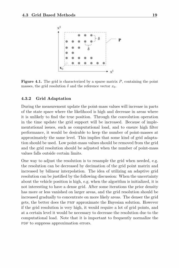
The grid is characterized by a matrix containing the point masses, a resolu-tion and a reference vector. Usually not all of the grid points are occupiedby a nonzero point mass and thus the matrix will be rather sparse. Figure4.1 shows an example of how this might look like.Assume that the grid resolution is δ and the total number of grid points (inR2) is N , then the point-mass filter is described by the following equations(see e.g. [1]):
Algorithm 1 (The Point-Mass Filter)
ct =N∑
n=1
pet(yt − h(xt(k)))p(xt(k)|Yt−1)δ2 (4.13a)
p(xt(k)|Yt) =1ct
pet(yt − h(xt(k)))p(xt(k)|Yt−1) (4.13b)
xmmst =
N∑n=1
xt(n)p(xt(n)|Yt)δ2 (4.13c)
Pt =N∑
n=1
(xt(n) − xt)(xt(n) − xt)T p(xt(n)|Yt)δ2 (4.13d)
xt+1(k) = xt(k) + ut, k = 1, 2, . . . , N (4.13e)
p(xt+1(k)|Yt) =N∑
n=1
pvt(xt+1(k) − xt(n) − ut)p(xt(n)|Yt)δ2 (4.13f)
The equations (4.13a)-(4.13d) is often referred to as the measurement up-date. During these steps the point-masses are re-weighted according to theinformation in the new measurement and the estimate and its error covari-ance are calculated. The next two steps, equations (4.13e) and (4.13f), arecalled the time update. First the grid points are translated according tothe relative movement ut and then the prior density is convolved with thedensity of vt, i.e. the prior density is smoothed somewhat due to the uncer-tainty in the relative movement. A more detailed presentation of the pmfis given in [1].
4.3 Grid Based Methods 19
Figure 4.1. The grid is characterized by a sparse matrix P , containing the pointmasses, the grid resolution δ and the reference vector x0.
4.3.2 Grid Adaptation
During the measurement update the point-mass values will increase in partsof the state space where the likelihood is high and decrease in areas whereit is unlikely to find the true position. Through the convolution operationin the time update the grid support will be increased. Because of imple-mentational issues, such as computational load, and to ensure high filterperformance, it would be desirable to keep the number of point-masses atapproximately the same level. This implies that some kind of grid adapta-tion should be used. Low point-mass values should be removed from the gridand the grid resolution should be adjusted when the number of point-massvalues falls outside certain limits.
One way to adjust the resolution is to resample the grid when needed, e.g.the resolution can be decreased by decimation of the grid point matrix andincreased by bilinear interpolation. The idea of utilizing an adaptive gridresolution can be justified by the following discussion: When the uncertaintyabout the vehicle position is high, e.g. when the algorithm is initialized, it isnot interesting to have a dense grid. After some iterations the prior densityhas more or less vanished on larger areas, and the grid resolution should beincreased gradually to concentrate on more likely areas. The denser the gridgets, the better does the pmf approximate the Bayesian solution. Howeverif the grid resolution is very high, it would require a lot of grid points, andat a certain level it would be necessary to decrease the resolution due to thecomputational load. Note that it is important to frequently normalize thepdf to suppress approximation errors.
20 4 Bayesian Estimation
If N is the number of nonzero grid points, a simple adaptation procedurecan be described by the following steps:
• If N > N1, remove every second row and column from the matrix andset the resolution to 2δ.
• If N < N2, use bilinear interpolation to increase the number of ele-ments in the matrix and set the resolution to δ/2.
4.4 Monte Carlo Methods
An alternative to deterministic methods, such as the pmf, is to use a stochas-tic (simulation-based) approach.
4.4.1 Monte Carlo Integration
One class of simulation-based methods are the Monte Carlo methods. Theyaim at approximating integrals of the kind
I =∫
Rn
f(x)π(x) dx, (4.14)
where ∫Rn
π(x) dx = 1 , π(x) > 0 ∀x (4.15)
by the following sum
I =N∑
i=1
f(xi). (4.16)
The set xiNi=1 is i.i.d. (independent identically distributed) samples from
π(x). Some of the integrals of interest in the Bayesian solution, like themms estimate (4.9) and the error covariance (4.11), is of the kind in (4.14).
In general it is not possible to sample directly from the distribution π(x).However this can be tackled e.g. by using the following technique: Letq(x) be a distribution from which samples are easily generated. Then animportance weight can be defined for each sample from q(x) as
w(xi) =π(xi)q(xi)
(4.17)
Hence the density function q(x) is usually referred to as importance function.The integral in (4.14) can thus be rewritten as
4.4 Monte Carlo Methods 21
I =∫
Rn
f(x)π(x)q(x)
q(x) dx =∫
Rn
f(x)w(x)q(x) dx (4.18)
This integral can be approximated by
I =N∑
i=1
f(xi)w(xi), (4.19)
where xiNi=1 are i.i.d. samples from q(x).
The importance weights can be seen as correction factors when the valueof the density function q(x) does not agree with value of the true densityfunction π(x). This sampling technique is called importance sampling andthe performance is of course dependent on the choice of importance function.
In the Bayesian framework the target distribution is given by
π(x) = p(x|y) ∝ p(y|x)p(x). (4.20)
If the prior distribution, p(x), is used as importance function, the unnor-malized weights is given by w(x) = p(y|x). A more detailed presentation ofMonte Carlo methods are given in [1] and [4].
4.4.2 Sequential Monte Carlo Methods
If Monte Carlo integration is used in a recursive estimation problem, thetarget distribution, π(x), is time dependent
πt(xt) = p(xt|Yt). (4.21)
In general there exists no explicit analytical expression for this function.This means that recursive, or sequential, Monte Carlo methods have to dealwith approximation and propagation of the posterior density function aswell. This is achieved by representing it with a set of i.i.d. samples drawnfrom (4.21) (or approximately by using e.g. importance sampling). Thesesamples are often called particles, because of their similarity with a swarm orcloud of small particles (e.g. dust) that evolves with time, when propagatedaccording to the Bayesian solution. The filters based on sequential MonteCarlo methods are thus often referred to as particle filters.
A major advantage of Monte Carlo methods over numerical integration isthat the complexity of the problem does not increase as much with the state
22 4 Bayesian Estimation
dimension. This can be motivated by the fact that in Monte Carlo integra-tion the samples of the posterior distribution are automatically chosen inthe parts of the state space that are important for the integration result.This means that the grid is adaptive in an efficient way and that the userdoes not have to bother about how to discretize the state space.
4.4.3 Particle Filters
One algorithm that utilizes the sequential Monte Carlo ideas is the Bayesianbootstrap or Sampling Importance Resampling (sir) filter [1, 4, 8] summa-rized in Algorithm 2.
Algorithm 2 (Bayesian bootstrap (SIR))
1. Set t = 0 and sample N times from p(x0) to generate the set xi0N
i=1
2. Calculate normalized weights wi = pet (yt−h(xit))∑N
j=1 pet (yt−h(xjt ))
.
3. Calculate position estimate xMMSt =
∑Ni=1 wix
it.
4. Generate a new set xi∗0 N
i=1 by sampling with replacement N timesfrom the old set. The probability for resampling particle xj
t should beequal to wj.
5. Generate vit ∼ pvt(v), i = 1, . . . , N
and predict each particle xit+1 = xi
t + ut + vit, i = 1, . . . , N
6. Set t = t + 1 and iterate from 2.
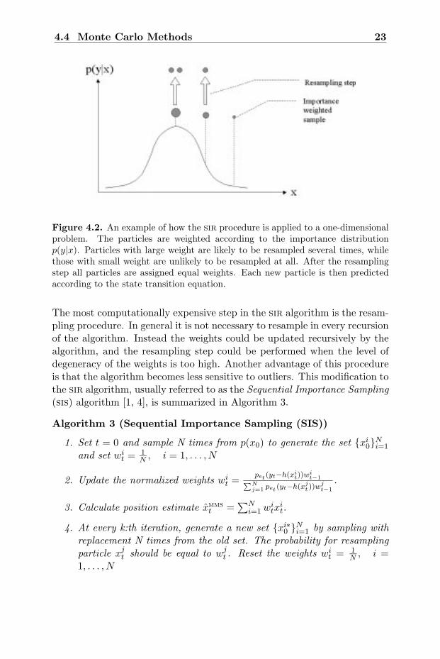
The algorithm is initialized by generating samples from the prior distribu-tion, p(x0). The samples are then weighted with the information providedby the measurement. These weights are used to estimate the position andthe error covariance. The next step is to propagate the posterior distribu-tion. This is done by resampling with replacement (the bootstrap step) fromthe present set of samples. The probability of resampling a certain particleis equal to its importance weight. This means that particles with a smallweight will most likely not be resampled. Such particles are “killed” in theresampling step, while particles with a large weight probably will be resam-pled several times, and thus new particles will be “born” in areas where it islikely to find the true position. The recursion is ended with a time updateor prediction step, where every particle is translated according to the statetransition equation. The sir procedure is illustrated in Figure 4.2.
4.4 Monte Carlo Methods 23
Figure 4.2. An example of how the sir procedure is applied to a one-dimensionalproblem. The particles are weighted according to the importance distributionp(y|x). Particles with large weight are likely to be resampled several times, whilethose with small weight are unlikely to be resampled at all. After the resamplingstep all particles are assigned equal weights. Each new particle is then predictedaccording to the state transition equation.
The most computationally expensive step in the sir algorithm is the resam-pling procedure. In general it is not necessary to resample in every recursionof the algorithm. Instead the weights could be updated recursively by thealgorithm, and the resampling step could be performed when the level ofdegeneracy of the weights is too high. Another advantage of this procedureis that the algorithm becomes less sensitive to outliers. This modification tothe sir algorithm, usually referred to as the Sequential Importance Sampling(sis) algorithm [1, 4], is summarized in Algorithm 3.
Algorithm 3 (Sequential Importance Sampling (SIS))
1. Set t = 0 and sample N times from p(x0) to generate the set xi0N
i=1
and set wit = 1
N , i = 1, . . . , N
2. Update the normalized weights wit =
pet (yt−h(xit))w
it−1∑N
j=1 pet (yt−h(xjt ))w
jt−1
.
3. Calculate position estimate xmmst =
∑Ni=1 wi
txit.
4. At every k:th iteration, generate a new set xi∗0 N
i=1 by sampling withreplacement N times from the old set. The probability for resamplingparticle xj
t should be equal to wjt . Reset the weights wi
t = 1N , i =
1, . . . , N
24 4 Bayesian Estimation
5. Generate vit ∼ pvt(v), i = 1, . . . , N
and predict each particle xit+1 = xi
t + ut + vit, i = 1, . . . , N
6. Set t = t + 1 and iterate from 2.
Instead of inserting the bootstrap step on regular basis (every k:th itera-tion) one could do this only when a significant degeneracy of the weights isobserved. A measure for determining the level of degeneracy is the effectivesample size [1, 4] which can be estimated by
Neff =1∑N
j=1 wjt
2 (4.22)
If all the particles have the same weight this expression yields the truesample size (N). When the algorithm starts to degenerate the variance ofthe weights increases and this is reflected in the denominator of (4.22). Thebootstrap step is applied when Neff falls below a certain threshold, Nthres ,defined by the user.
5 Vehicle Positioning 25
5 Vehicle Positioning
The filters presented in the previous sections provide approximations to theoptimal Bayesian solution. The next step is to implement and evaluatethese filters when applied to the vehicle positioning problem.
When initializing the filters it is assumed that some knowledge about theinitial position is available, i.e. one knows that the true initial position iswithin some limited region of the map. This information can be obtainede.g. by restoring a saved position or by using a single position fix from anexternal system like the cellular radio network. In either case the accuracyof this initial estimate is allowed to be rather poor.
Furthermore, the true orientation of the vehicle is assumed to be known.This means that the input from the dead-reckoning system can be treatedas a relative displacement vector in the coordinate system of the map, see(3.4).
5.1 Implementation
5.1.1 The Point-Mass Filter
The pmf has been implemented in the matlabtm [10] environment, using asparse matrix representation, i.e. only non-zero grid points and their indicesare stored and operated on. The implementation used is almost identicalwith the one suggested in [1].
The performance of the filter depends on several factors. Since it is desirableto achieve both low approximation errors and low computational load, it willbe necessary to make a trade-off. As discussed in Section 4.3.2 the densityof the grid is a tuning parameter for this purpose. Other aspects that haveto be considered are for example:
• The choice of prior distribution.
• Should the grid be adaptive with time? How should it be adapted? Isthere a significant performance gain?
• The choice of noise distributions and variance.
• The memory requirements, i.e. how large support can the grid haveand how dense can it be?
• Robustness against e.g. measurement errors and sensor drifts.
26 5 Vehicle Positioning
5.1.2 The Particle Filter
Several versions of the particle filter were implemented in matlabtm includ-ing some modifications discussed further in Section 5.2.3, though the basicalgorithm was the standard sir algorithm.
An interesting implementational issue is the number of particles used in thealgorithm. Either one can choose to have a fixed number throughout thewhole run, or to utilize an adaptive sample size. The latter choice can bejustified by the fact that a large number of particles is in general requiredinitially, but when the algorithm has converged a smaller number will suffice.In [3] a lower bound for the number of particles required to assure a certainquality of the approximation is derived.
Even though there is a possibility to decrease the number of particles duringthe execution of the algorithm, it is not obvious that one should do that. Ifthe filter is to be implemented in a real-time environment it is often betterto have a fixed sample size for scheduling and memory allocation reasons.
5.2 Performance Evaluation
The pmf and the particle filter have been simulated on both fictitious andreal measurements.
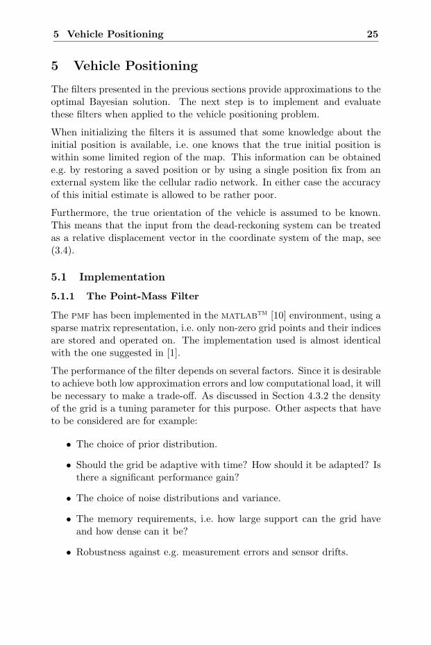
Preliminary simulations were performed on a simple, imaginary map usingsimulated measurement data. The pmf implementation seemed to work verywell with a fixed grid resolution. The particle filter on the other hand showeda rather disappointing performance. The frequency of filter divergence wasfar too high; in some cases over 20%. Even after convergence the filter couldsuddenly loose the track of the vehicle, resulting in a divergence. Figure 5.1shows how typical divergence of the particle filter might look like (in thiscase when applied to real measurement data).
Due to these discouraging results, effort was put into how to improve theparticle filter implementation. In Section 5.2.2 these issues are discussed indetail.
5.2.1 Measurement Data Acquisition
The measurement data used for the simulations were collected from testdrives in suburban and dense residential areas. The sensor equipment in-cluded abs signals (wheel speed) available through the can bus, a rate-gyro
5.2 Performance Evaluation 27
0 50 100 150 200 250 3000
50
100
150
200
250
300
Sample No
Err
or [m
]
Figure 5.1. The estimation error of 100 different simulations on the same sequenceof measurement data, using the particle filter (sir with a fixed number of particles,N=2000). In this case 22 of the runs did not converge, which is far too many.
oriented along the vertical axis and a three-dimensional accelerometer clus-ter. However, the accelerometer signals were not used here due to theirsensitivity to road inclination. A gps-receiver was used as absolute positionreference along the test path. The measurements were collected by a hard-ware platform mounted in the test vehicle, a Volvo V40, and downloadedto a laptop.
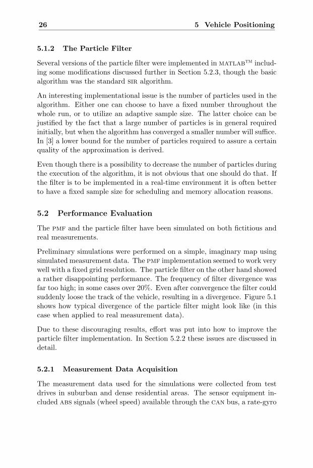
In this report, two different data sets were used for evaluation purposes.The first one, in the sequel referred to as S1, is a 560 seconds long sequencecollected in a suburban district (Figure 5.2(a)). The second one was col-lected in a denser residential area with several crossings (Figure 5.2(b)).This sequence will be referred to as S2.
The signals were sampled with 20 Hz, but in the simulations they wereresampled with 2 Hz. The gyro offset was removed off-line since the mainobjective here is not to test the robustness of the filters.
To provide the filters with maps of the test drive areas, a simple digitizinggui was implemented in matlabtm. The road network was then encodedfrom high resolution (1 m/pixel) aerial photos.
28 5 Vehicle Positioning
(a) Test drive S1. (b) Test drive S2.
Figure 5.2. The test drives used in the simulations.
5.2.2 Particle Clustering
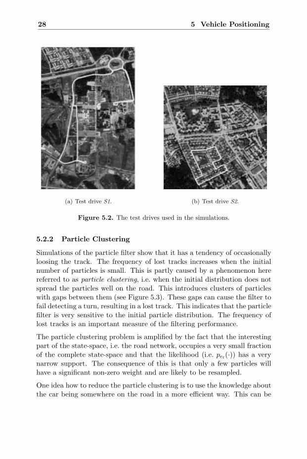
Simulations of the particle filter show that it has a tendency of occasionallyloosing the track. The frequency of lost tracks increases when the initialnumber of particles is small. This is partly caused by a phenomenon herereferred to as particle clustering, i.e. when the initial distribution does notspread the particles well on the road. This introduces clusters of particleswith gaps between them (see Figure 5.3). These gaps can cause the filter tofail detecting a turn, resulting in a lost track. This indicates that the particlefilter is very sensitive to the initial particle distribution. The frequency oflost tracks is an important measure of the filtering performance.
The particle clustering problem is amplified by the fact that the interestingpart of the state-space, i.e. the road network, occupies a very small fractionof the complete state-space and that the likelihood (i.e. pet(·)) has a verynarrow support. The consequence of this is that only a few particles willhave a significant non-zero weight and are likely to be resampled.
One idea how to reduce the particle clustering is to use the knowledge aboutthe car being somewhere on the road in a more efficient way. This can be
5.2 Performance Evaluation 29
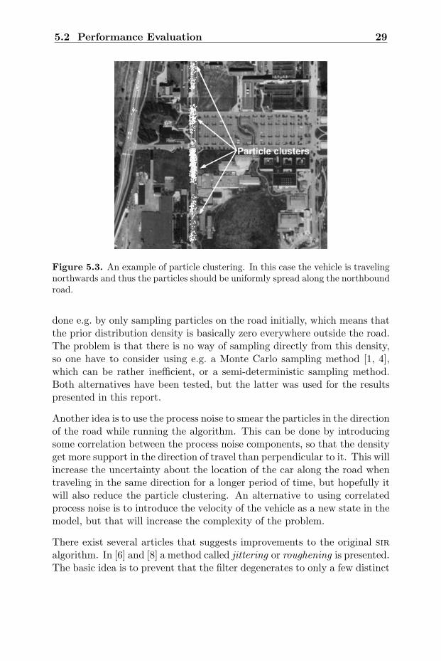
Figure 5.3. An example of particle clustering. In this case the vehicle is travelingnorthwards and thus the particles should be uniformly spread along the northboundroad.
done e.g. by only sampling particles on the road initially, which means thatthe prior distribution density is basically zero everywhere outside the road.The problem is that there is no way of sampling directly from this density,so one have to consider using e.g. a Monte Carlo sampling method [1, 4],which can be rather inefficient, or a semi-deterministic sampling method.Both alternatives have been tested, but the latter was used for the resultspresented in this report.
Another idea is to use the process noise to smear the particles in the directionof the road while running the algorithm. This can be done by introducingsome correlation between the process noise components, so that the densityget more support in the direction of travel than perpendicular to it. This willincrease the uncertainty about the location of the car along the road whentraveling in the same direction for a longer period of time, but hopefully itwill also reduce the particle clustering. An alternative to using correlatedprocess noise is to introduce the velocity of the vehicle as a new state in themodel, but that will increase the complexity of the problem.
There exist several articles that suggests improvements to the original siralgorithm. In [6] and [8] a method called jittering or roughening is presented.The basic idea is to prevent that the filter degenerates to only a few distinct
30 5 Vehicle Positioning
sample values (i.e. to prevent clusters) by adding some noise to each samplegenerated in the time update step. This is particularly efficient when theprocess noise is low.
Another method is prior editing [6, 8], which uses an acceptance test afterthe sampling step. This means that only samples with a reasonable chanceof being resampled is accepted. To achieve this one needs to have access tothe next measurement, which will delay the estimate one sample.
5.2.3 Improvements of the Particle Filter Implementation
A solution to the particle clustering problem discussed in the previous sec-tion is to introduce some correlation in the noise distribution, which is usedin the state evolution equation (3.1), vt. The aim is to spread more particlesalong the road rather than away from it. If one assume that the absoluteheading of the vehicle, i.e. the Euler yaw angle ψt, is known and Gaussiannoise is used, the noise vector expressed in the vehicle-body frame,
v′t =[
vlatt
vlongt
](5.1)
can be transformed to the global frame
vt =[
cos ψt − sinψt
sinψt cos ψt
]v′t. (5.2)
By choosing the variance of vlatt and vlong
t , the desired particle distributioncan be tuned.
Yet another modification to improve the particle convergence is to introducea prior editing step in the time update of the particle filter. The prior editingprocedure involves an acceptance test after the bootstrap step as describedby Algorithm 4. Note that this modifies item 4 and 5 in Algorithm 2 and 3.
Algorithm 4 (Prior Editing)
1. Set i=1.
2. Generate a sample xi∗t in the bootstrap step (i.e. xi∗
t is assumed tobe an i.i.d. sample from p(xt|Yt)) and predict xi
t+1 = xi∗t + ut + vi
t,vit ∼ pvt(v).
3. Calculate the residual eit+1 = yt+1 − h(xi
t+1)
5.2 Performance Evaluation 31
4. Accept this sample and set i = i + 1 if |eit+1| < kpe
√Var(et), where
kpe is a user defined parameter.
5. Iterate from item 2 while i ≤ N
Note that the prior editing requires the next measurement yt+1 and that thiswould delay the filter one sample. However, since the measurement in thiscase is rather fictitious and considered to be known for all time instances(see Section 3.2), no time lag is introduced in the algorithm.
The relative number of rejected samples in the prior editing step is a measureof how well the particles are spread onto the road. When the vehicle ismaking a sharp turn the prior editing ratio will increase slightly, becausemost particles are spread in the direction of the tangent to the trajectory.
5.2.4 Evaluation Using Real Measurements
The pmf was simulated on data from S1, using a fixed grid resolution, δ = 5m, and N = 40 000 grid points initially. The position error compared tothe gps is shown in figure 5.4. Also included in the figure is the square rootof the scalar mean square error, which is defined by
E(∥∥xt − xt
∥∥2
2
)= tr Pt, (5.3)
which can be thought of as the standard deviation of the estimation error[9]. The “true” position, xt, was obtained from dead reckoning using off-line corrected sensor signals, i.e. the sensor errors were tuned so that thetrajectory of the vehicle matched the current driving path on the map.
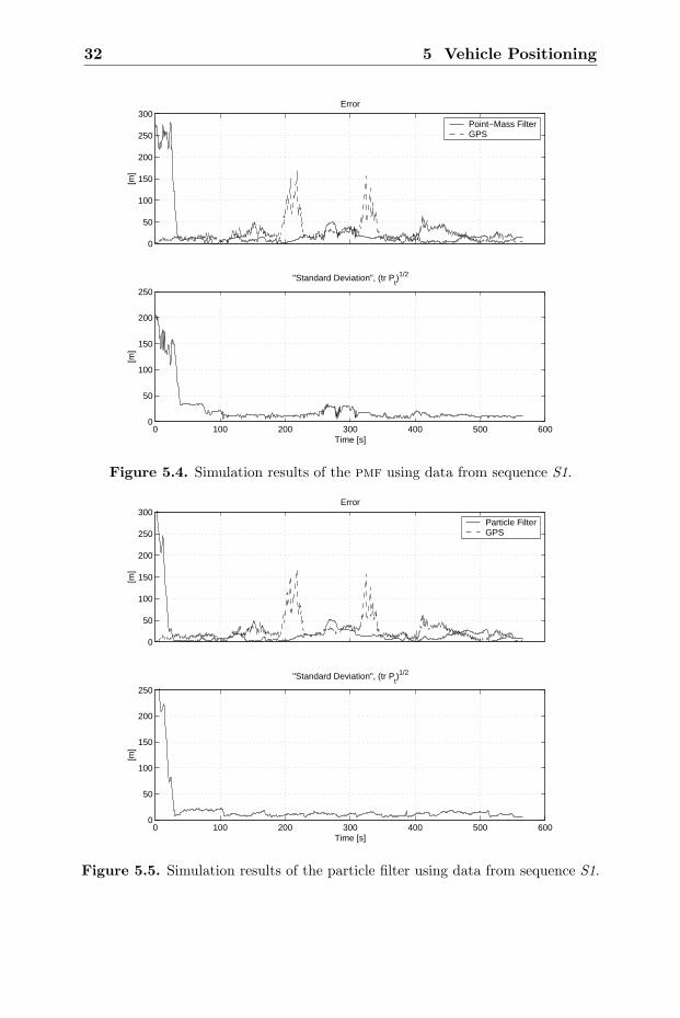
The increase in the error after about 280 seconds is caused by off-roaddriving. The large error in the gps-position in some regions arises whendriving under foliage. The position estimate from the pmf is better thanthe gps-position almost everywhere during the simulation.
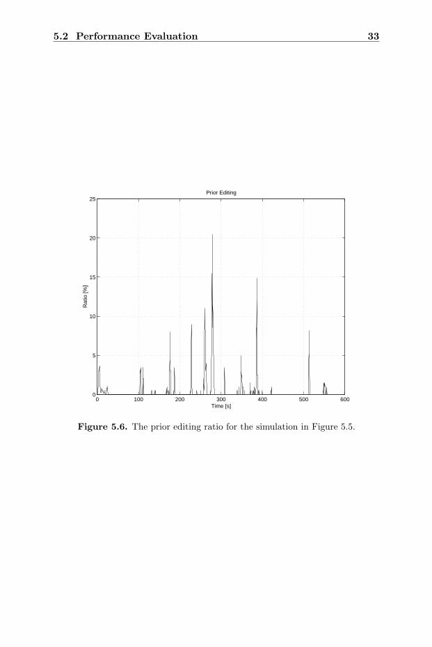
A simulation on the same sequence, performed with the particle filter usingprior editing, is shown in Figure 5.5. The relative number of rejected samplesin the prior editing step is shown in Figure 5.6.
32 5 Vehicle Positioning
0
50
100
150
200
250
300Error
[m]
Point−Mass FilterGPS
0 100 200 300 400 500 6000
50
100
150
200
250
"Standard Deviation", (tr Pt)1/2
Time [s]
[m]
Figure 5.4. Simulation results of the pmf using data from sequence S1.
0
50
100
150
200
250
300Error
[m]
Particle FilterGPS
0 100 200 300 400 500 6000
50
100
150
200
250
"Standard Deviation", (tr Pt)1/2
[m]
Time [s]
Figure 5.5. Simulation results of the particle filter using data from sequence S1.
5.2 Performance Evaluation 33
0 100 200 300 400 500 6000
5
10
15
20
25Prior Editing
Time [s]
Rat
io [%
]
Figure 5.6. The prior editing ratio for the simulation in Figure 5.5.
34 5 Vehicle Positioning
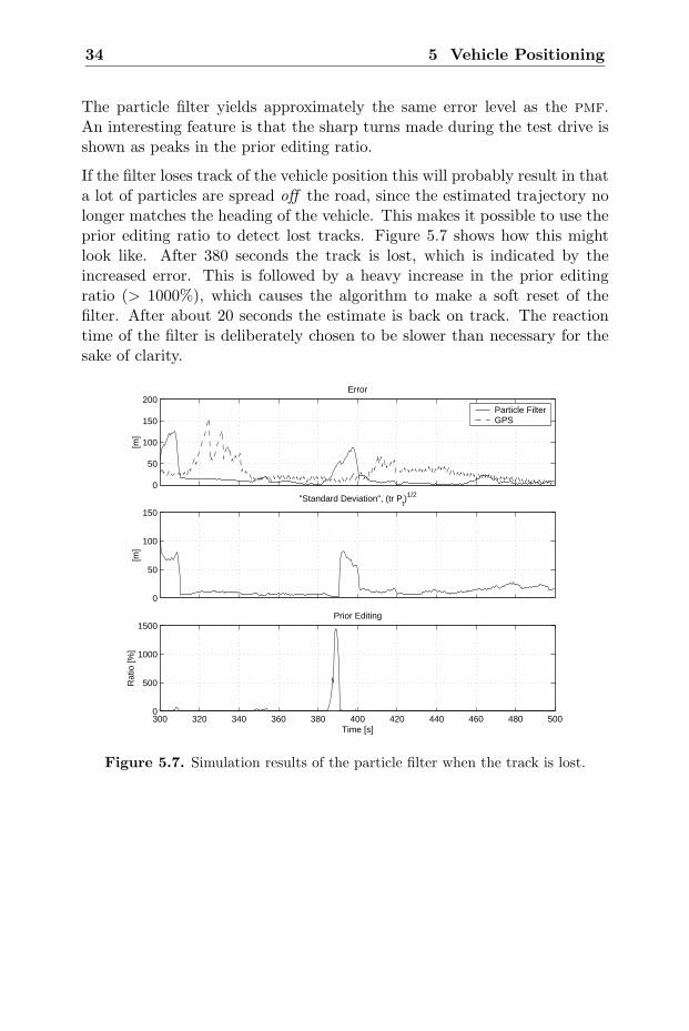
The particle filter yields approximately the same error level as the pmf.An interesting feature is that the sharp turns made during the test drive isshown as peaks in the prior editing ratio.
If the filter loses track of the vehicle position this will probably result in thata lot of particles are spread off the road, since the estimated trajectory nolonger matches the heading of the vehicle. This makes it possible to use theprior editing ratio to detect lost tracks. Figure 5.7 shows how this mightlook like. After 380 seconds the track is lost, which is indicated by theincreased error. This is followed by a heavy increase in the prior editingratio (> 1000%), which causes the algorithm to make a soft reset of thefilter. After about 20 seconds the estimate is back on track. The reactiontime of the filter is deliberately chosen to be slower than necessary for thesake of clarity.
0
50
100
150
200Error
[m]
Particle FilterGPS
0
50
100
150
"Standard Deviation", (tr Pt)1/2
[m]
300 320 340 360 380 400 420 440 460 480 5000
500
1000
1500Prior Editing
Time [s]
Rat
io [%
]
Figure 5.7. Simulation results of the particle filter when the track is lost.
5.2 Performance Evaluation 35
5.2.5 Monte Carlo Simulations
To evaluate the performance of the particle filter, extensive simulationsare required because of its stochastic nature3. However, by applying thealgorithm several times to a single data set, each time with a different noiserealization, a similar effect can be achieved. This kind of simulation is calledMonte Carlo simulation [9].
Suppose that M Monte Carlo runs are generated from one set of measure-ment data, i.e. M different sequences of position estimates are available.Then it is possible to calculate the root mean square error (rmse) fromthese simulations
rmse(t) =
1
M
M∑j=1
∥∥xt − x(j)t
∥∥2
2
1/2
(5.4)
which is a measure of the length (magnitude) of the estimation error, i.e.the distance between the estimated and the true position. A common navi-gation performance parameter is the median of this error, the circular errorprobable (cep).
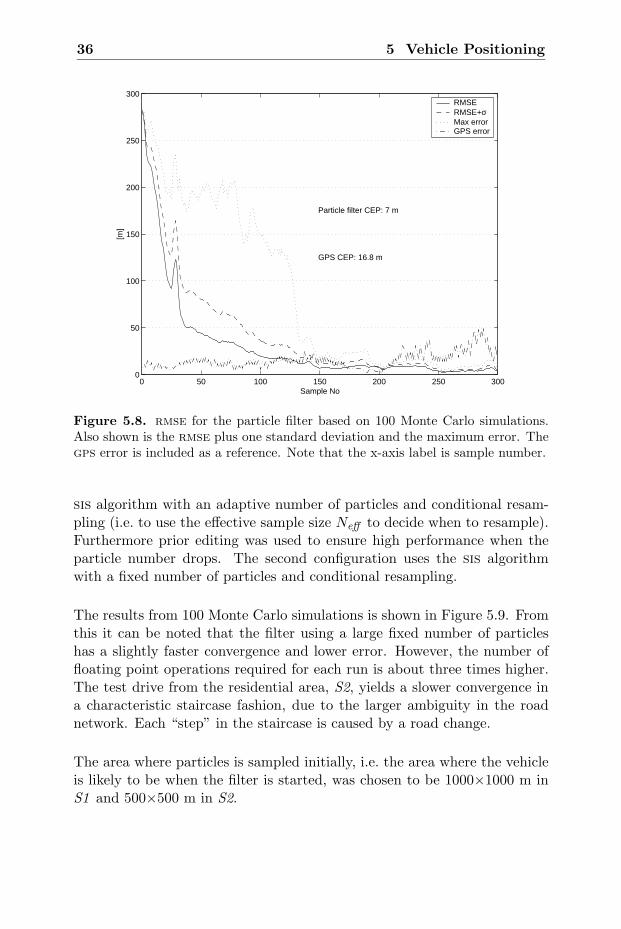
Results from 100 Monte Carlo simulations of the particle filter (sir withcorrelated process noise and prior editing) using data from test drive S1are shown in Figure 5.8. The number of particles used in each recursionwas chosen adaptively between 200 and 1000, based on the uncertainty inthe estimate. The cep was calculated for the sequence starting after aburn-in4 time, i.e. in this case after about 150 samples, and compared tothe corresponding value obtained from the gps. Since the gps-receiver hastrouble with foliage at the end of the sequence, the particle filter yieldssignificantly better performance.
It should be noted that the gps receiver has an initial transient as well,although not shown in the results. For the particular receiver model usedhere the initialization process takes approximately 45 seconds.
The particle filter can be configured in several ways, using the ideas dis-cussed in Section 5.2.3. However, this report will only present a selectionof these. Two different configurations have been simulated on measurementdata from the driving scenarios depicted in Figure 5.2. The first one uses the
3This can be motivated by Figure 5.1; the true performance of the filter is not revealedby a single simulation.
4The transient of the estimation error.
36 5 Vehicle Positioning
0 50 100 150 200 250 3000
50
100
150
200
250
300
Sample No
[m]
Particle filter CEP: 7 m
GPS CEP: 16.8 m
RMSE RMSE+σMax error GPS error
Figure 5.8. rmse for the particle filter based on 100 Monte Carlo simulations.Also shown is the rmse plus one standard deviation and the maximum error. Thegps error is included as a reference. Note that the x-axis label is sample number.
sis algorithm with an adaptive number of particles and conditional resam-pling (i.e. to use the effective sample size Neff to decide when to resample).Furthermore prior editing was used to ensure high performance when theparticle number drops. The second configuration uses the sis algorithmwith a fixed number of particles and conditional resampling.
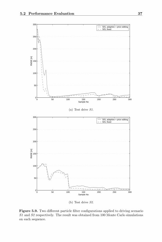
The results from 100 Monte Carlo simulations is shown in Figure 5.9. Fromthis it can be noted that the filter using a large fixed number of particleshas a slightly faster convergence and lower error. However, the number offloating point operations required for each run is about three times higher.The test drive from the residential area, S2, yields a slower convergence ina characteristic staircase fashion, due to the larger ambiguity in the roadnetwork. Each “step” in the staircase is caused by a road change.
The area where particles is sampled initially, i.e. the area where the vehicleis likely to be when the filter is started, was chosen to be 1000×1000 m inS1 and 500×500 m in S2.
5.2 Performance Evaluation 37
0 50 100 150 200 250 3000
50
100
150
200
250
300
Sample No
RM
SE
[m]
SIS, adaptive + prior editingSIS, fixed
(a) Test drive S1.
0 50 100 150 200 250 3000
50
100
150
200
250
300
Sample No
RM
SE
[m]
SIS, adaptive + prior editingSIS, fixed
(b) Test drive S2.
Figure 5.9. Two different particle filter configurations applied to driving scenarioS1 and S2 respectively. The result was obtained from 100 Monte Carlo simulationson each sequence.
38 5 Vehicle Positioning
5.3 Discussion
Both the pmf and the particle filter solves the vehicle positioning prob-lem with satisfying performance. The particle filter occasionally diverges,but the frequency of these events can be reduced by some improvements,like e.g. correlated process noise, semi-deterministic prior distribution andprior editing. The latter of these modifications also provides a method ofdetecting filter divergence, so that the algorithm can be re-initialized.
A major drawback of the filters discussed so far is that the heading anglemust be provided by an external source. Hence, the robustness againstangular errors are low. If e.g. there is a drift in the heading angle, thealgorithms will most certainly diverge.
The simulations discussed above assume that the initial knowledge aboutthe position is very uncertain. In general, when the filters are started, it ispossible to retrieve a stored position and thus the initial estimate is muchbetter than the ones considered here.
Since the map-aided approach heavily relies on the accuracy of the map,an important question is how the map should be modeled to yield optimalperformance of the algorithms. Although this thesis does not focus on theseaspects, one should keep in mind that map modeling errors have a greatinfluence on the performance of this method.
6 Heading Angle Estimation 39
6 Heading Angle Estimation
The algorithms presented in the previous section solve the two-dimensionalpositioning problem, assuming that the heading angle is known. A naturalextension would be to explore the possibilities to remove that assumptionin order to get an independent absolute position estimator.
The extended estimation problem includes estimation of the heading angleand thus the state-space model has to be modified.
6.1 Model Extension
The two-dimensional state space model assumes that the absolute headingof the vehicle is known and thus this information has to be provided froman external source. However, since the map contains a lot more informationthan used in the current model, there is a possibility to estimate the headingangle as well. To be able to do this, an extension of the model is needed.Let the heading angle be denoted by ψt and introduce it as a new state
xt+1 = xt + f(ψt, ∆r) + vxt (6.1a)
ψt+1 = ψt + ∆ψ + vψt (6.1b)
y1t = h(xt) + e1
t (6.1c)y2
t = φ(xt, ψt) + e2t (6.1d)
where the input from the relative sensors are split up into a linear and anangular displacement, i.e.
∆r = Tsvx (6.2)∆ψ = Tsψ (6.3)
The nonlinear function f(ψt, ∆r) is given by
f(ψt, ∆r) =[ −∆r sinψt
∆r cos ψt
](6.4)
The state evolution is no longer linear, but consists of a nonlinear updateof xt and a linear update of ψt. A new measurement, y2
t , is added as well.It consists of the nonlinear function, φ(xt, ψt), that yields the orientation of
40 6 Heading Angle Estimation
the closest road minus the current heading angle, plus some measurementnoise.
The Bayesian solution to the three-dimensional problem is of course some-what different compared to the one presented in Section 4.2. However, thederivation is almost identical (see Appendix B) and thus the solution is justsummarized here as
p(xt|Y t) =1ct
pet(y1t − h(xt), y2
t − φt(xt) + ψt)p(xt|Y t−1) (6.5)
p(xt+1|Y t) =∫
R3
pvt(xt+1 − xt − f(ψt, ∆r), ψt+1 − ψt − ∆ψ)p(xt|Y t) dxt,
(6.6)where
xt =(
xt
ψt
), Y t =
y1
i , y2i
t
i=0.
Note that pvt is a three-dimensional pdf, while pet is two-dimensional.
6.2 Implementation
Since the extended estimation problem introduces an extra state in themodel, the complexity of the problem increases as well. Therefore, due toits special properties concerning high dimensional problems, the particlefilter is chosen for this purpose. Although the performance of Monte Carlomethods does not explicitly depend on the dimension of the problem, thenumber of particles usually has to be increased, especially during the initialphase. To relieve the computational load due to the increased sample size,the sis algorithm is utilized here. It should be noted that the original siralgorithm is a special case of sis when the bootstrap step is included inevery iteration.
6.3 Performance Evaluation
The filter was simulated on sensor data collected in both suburban areasand dense residential areas. No initial knowledge about the orientation isassumed, i.e. the initial heading angle is uniformly distributed between 0
and 360.
6.3 Performance Evaluation 41
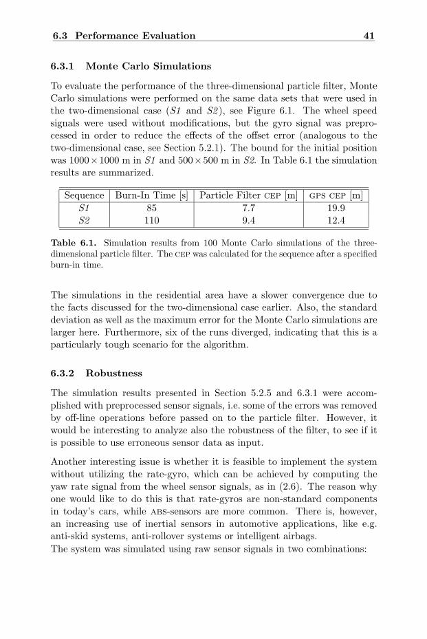
6.3.1 Monte Carlo Simulations
To evaluate the performance of the three-dimensional particle filter, MonteCarlo simulations were performed on the same data sets that were used inthe two-dimensional case (S1 and S2 ), see Figure 6.1. The wheel speedsignals were used without modifications, but the gyro signal was prepro-cessed in order to reduce the effects of the offset error (analogous to thetwo-dimensional case, see Section 5.2.1). The bound for the initial positionwas 1000×1000 m in S1 and 500×500 m in S2. In Table 6.1 the simulationresults are summarized.
Sequence Burn-In Time [s] Particle Filter cep [m] gps cep [m]S1 85 7.7 19.9S2 110 9.4 12.4
Table 6.1. Simulation results from 100 Monte Carlo simulations of the three-dimensional particle filter. The cep was calculated for the sequence after a specifiedburn-in time.
The simulations in the residential area have a slower convergence due tothe facts discussed for the two-dimensional case earlier. Also, the standarddeviation as well as the maximum error for the Monte Carlo simulations arelarger here. Furthermore, six of the runs diverged, indicating that this is aparticularly tough scenario for the algorithm.
6.3.2 Robustness
The simulation results presented in Section 5.2.5 and 6.3.1 were accom-plished with preprocessed sensor signals, i.e. some of the errors was removedby off-line operations before passed on to the particle filter. However, itwould be interesting to analyze also the robustness of the filter, to see if itis possible to use erroneous sensor data as input.
Another interesting issue is whether it is feasible to implement the systemwithout utilizing the rate-gyro, which can be achieved by computing theyaw rate signal from the wheel sensor signals, as in (2.6). The reason whyone would like to do this is that rate-gyros are non-standard componentsin today’s cars, while abs-sensors are more common. There is, however,an increasing use of inertial sensors in automotive applications, like e.g.anti-skid systems, anti-rollover systems or intelligent airbags.The system was simulated using raw sensor signals in two combinations:

42 6 Heading Angle Estimation
0 50 100 150 200 250 3000
50
100
150
200
250
300
350
Sample No
[m]
Particle filter CEP: 7.7 m
GPS CEP: 19.9 m
RMSE RMSE+σMax error GPS error
(a) Test drive S1.
0 50 100 150 200 250 3000
50
100
150
200
250
300
350
Sample No
[m] Particle filter CEP: 9.4 m
GPS CEP: 12.4 m
RMSE RMSE+σMax error GPS error
(b) Test drive S2.
Figure 6.1. 100 Monte Carlo simulations of the three-dimensional particle filterapplied to driving scenario S1 and S2 respectively.
6.3 Performance Evaluation 43
• Longitudinal velocity calculated from the abs-sensors and yaw rateprovided by the gyro.
• Both longitudinal velocity and yaw rate calculated from the abs-sensors.
Since the gyro signal is associated with an offset error, the heading anglewill suffer from linear drift. With the current error model this error can notbe completely eliminated. Hence, the estimated heading angle will includea small offset (Figure 6.2). One way to deal with this is to estimate thedrift, i.e. to include the drift term as a new state in the model. That willof course increase the dimension of the problem, but in this case there areways to simplify the computations [11].
0 20 40 60 80 100 120 140 160 180 200−2
−1.5
−1
−0.5
0
0.5
1
1.5
2
Time [s]
ψ [r
ad]
True Estimated
Figure 6.2. Estimated heading angle when the gyro signal was used (sequenceS1 ). Note that there is a small offset after burn-in.
If one instead uses the abs-sensor signals to calculate the yaw rate, thedrift is not as significant and thus the estimate is less biased (Figure 6.3).However, this is only true when the rear wheel radii are approximately thesame, which may not be the case if the tire pressure difference is significant.
This difference between the two sensor configurations has no significant
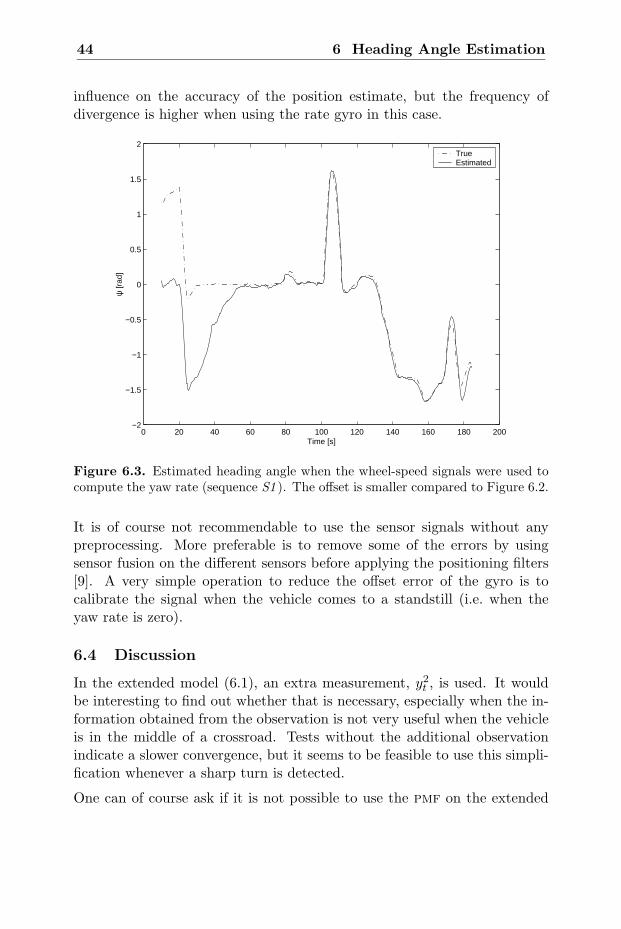
44 6 Heading Angle Estimation
influence on the accuracy of the position estimate, but the frequency ofdivergence is higher when using the rate gyro in this case.
0 20 40 60 80 100 120 140 160 180 200−2
−1.5
−1
−0.5
0
0.5
1
1.5
2
Time [s]
ψ [r
ad]
True Estimated
Figure 6.3. Estimated heading angle when the wheel-speed signals were used tocompute the yaw rate (sequence S1 ). The offset is smaller compared to Figure 6.2.
It is of course not recommendable to use the sensor signals without anypreprocessing. More preferable is to remove some of the errors by usingsensor fusion on the different sensors before applying the positioning filters[9]. A very simple operation to reduce the offset error of the gyro is tocalibrate the signal when the vehicle comes to a standstill (i.e. when theyaw rate is zero).
6.4 Discussion
In the extended model (6.1), an extra measurement, y2t , is used. It would
be interesting to find out whether that is necessary, especially when the in-formation obtained from the observation is not very useful when the vehicleis in the middle of a crossroad. Tests without the additional observationindicate a slower convergence, but it seems to be feasible to use this simpli-fication whenever a sharp turn is detected.
One can of course ask if it is not possible to use the pmf on the extended

6.4 Discussion 45
problem, when it seemed to work so well for the two-dimensional case.Theoretically, the corresponding procedure is to define a three-dimensionalgrid and apply the point-mass approximation. This means that a two-dimensional grid has to be used for each discretized value of the extendedstate variable (the heading angle). As can be imagined this entails a heavycomputational burden and large memory requirements.

46 6 Heading Angle Estimation
7 Conclusions 47
7 Conclusions
In this thesis we have studied map-aided vehicle positioning using Bayesianestimation. Sequential Monte Carlo methods as well as a numerical in-tegration method (the point-mass filter) have been successfully applied tothe basic two-dimensional positioning problem (assuming that the headingangle is known).
The extended problem, in which the heading angle is estimated as well asthe position, has been solved using a particle filter with satisfying results.
The conclusion of this work is that it is possible to use the concept ofmap-aided positioning, as defined in this report, in a vehicle positioningapplication. However, it needs a lot more research to be fully functional.
8 Future Work
The natural aim for the future work on this project is to implement the posi-tioning algorithm in a real-time environment for online evaluation. However,there are several other issues that should be further considered, e.g. the maprepresentation. In this thesis the maps have been digitized manually by theauthor. This procedure is of course not feasible in the long run and thereforeit is necessary to find a supplier of the desired map information.
Another aspect that should be investigated further is the robustness of thefilters. This requires extensive simulations and a lot of effort put on tuning.If the algorithm is to be implemented online, research on the computationalrequirements for different filter configurations has to be performed.
There are several possibilities for how the positioning algorithm could beused in a navigation system. One example is to use map-aided positioningtogether with a cellular radio positioning system. Another alternative isto add a magnetic compass to this configuration, and use the map-aidedalgorithm on the two-dimensional problem only. Yet another possibility isto use the map-aided positioning module as a complementary system to agps-based navigator, in order to increase the overall performance.
Apart from navigation applications, the map-aided positioning system canbe used for several other purposes. For example the heading angle estima-tion yields an improved yaw rate estimate, which is of great importancein anti-skid systems and many other automotive applications. The systemcan also be used for on-line sensor calibration, improved absolute velocityestimation and tire pressure indicators.
48 References
The ideas of map-aided positioning are of course not restricted only to roadvehicles (cars, busses, trucks, motorcycles), but can also be applied to otherareas where map information is available, such as e.g. trains and autonomousindustrial robots. The special requirements and problems associated withthis remains to be sorted out.
To summarize, the guideline in this work has been to use low cost sensorequipment and digitally stored maps to provide high performance position-ing for road vehicles. The nonlinear filtering problem that arises can be effi-ciently tackled by Bayesian estimation methods, as indicated by the resultspresented in this report. Thus the first stepping-stone has been completedand the next phase of this project can be initialized.
References
[1] N. Bergman. Recursive Bayesian Estimation: Navigation and TrackingApplications. PhD thesis, Linkoping University, May 1999.
[2] D. Bernstein and A. Kornhauser. An introduction to map matchingfor personal navigation assistants. Technical report, New Jersey TIDECenter, Princeton University, 1996. www.njtide.org.
[3] Y. Boers. On the number of samples to be drawn in particle filter-ing. IEE Colloquium on Target Tracking: Algorithms and Applications,215:5/1–5/6, 1999.
[4] A. Doucet, S.J. Godsill, and C. Andrieu. On sequential Monte Carlosampling methods for Bayesian filtering. Statistics and Computing,10(3):197–208, 2000.
[5] C. Drane, M. Macnaughtan, and C. Scott. Positioning GSM telephones.IEEE Communications Magazine, 36(4), 1998.
[6] P. Fearnhead. Sequential Monte Carlo methods in filter theory. PhDthesis, University of Oxford, 1998.
[7] T. Gillespie. Fundamentals of Vehicle Dynamics. Society of AutomotiveEngineers, Inc., 1992.
[8] N.J. Gordon, D.J. Salmond, and A.F.M. Smith. Novel approach tononlinear/non-Gaussian Bayesian state estimation. IEE Procedings onRadar and Signal Processing, 140:107–113, 1993.

References 49
[9] F. Gustafsson. Adaptive Filtering and Change Detection. John Wiley& Sons, Ltd, 2000.
[10] The MathWorks, Inc. MATLAB: Language Reference Manual, Version5, 1996.
[11] P.J. Nordlund. Recursive state estimation of nonlinear systems withapplications to integrated navigation. Technical Report LiTH-ISY-R-2321, Department of Electrical Engineering, Linkoping University,2000.
[12] Y. Zhao. Vehicle Location and Navigation Systems. Artech HousePublishers, 1997.
50 Appendix A: Bayes’ Rule
Appendix A: Bayes’ Rule
Let x and y denote two stochastic variables with probability density func-tions p(x) and p(y) respectively. The joint density can thus be written as
p(x, y) = p(x|y)p(y), (A.1)
or equivalently as
p(x, y) = p(y|x)p(x). (A.2)
Combining (A.1) and (A.2), and solving for the conditional probabilityp(x|y) yields
p(x|y) =p(y|x)p(x)
p(y). (A.3)
This expression is usually referred to as Bayes’ rule or Bayes’ theorem. Thedenominator p(y) can be obtained by marginalizing out x in (A.2)
p(y) =∫
Rn
p(x, y) dx =∫
Rn
p(y|x)p(x) dx. (A.4)
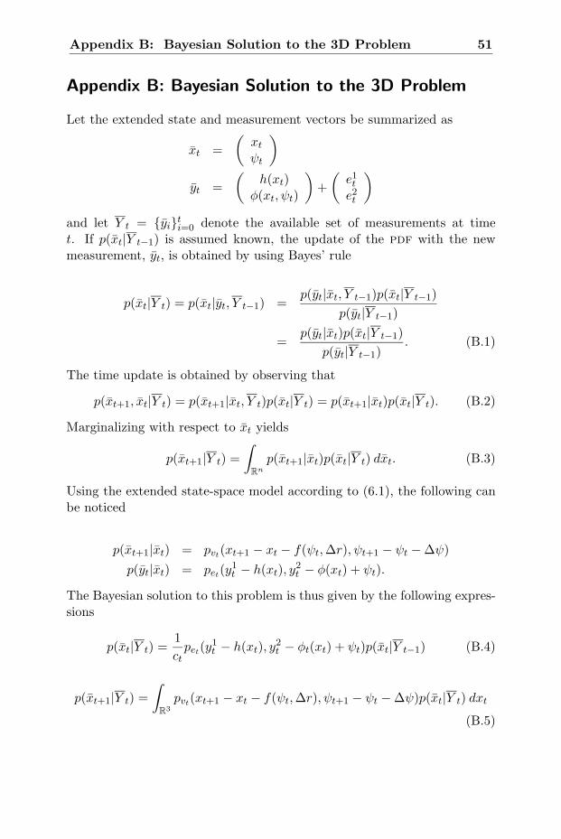
Appendix B: Bayesian Solution to the 3D Problem 51
Appendix B: Bayesian Solution to the 3D Problem
Let the extended state and measurement vectors be summarized as
xt =(
xt
ψt
)
yt =(
h(xt)φ(xt, ψt)
)+
(e1t
e2t
)
and let Y t = yiti=0 denote the available set of measurements at time
t. If p(xt|Y t−1) is assumed known, the update of the pdf with the newmeasurement, yt, is obtained by using Bayes’ rule
p(xt|Y t) = p(xt|yt, Y t−1) =p(yt|xt, Y t−1)p(xt|Y t−1)
p(yt|Y t−1)
=p(yt|xt)p(xt|Y t−1)
p(yt|Y t−1). (B.1)
The time update is obtained by observing that
p(xt+1, xt|Y t) = p(xt+1|xt, Y t)p(xt|Y t) = p(xt+1|xt)p(xt|Y t). (B.2)
Marginalizing with respect to xt yields
p(xt+1|Y t) =∫
Rn
p(xt+1|xt)p(xt|Y t) dxt. (B.3)
Using the extended state-space model according to (6.1), the following canbe noticed
p(xt+1|xt) = pvt(xt+1 − xt − f(ψt, ∆r), ψt+1 − ψt − ∆ψ)p(yt|xt) = pet(y
1t − h(xt), y2
t − φ(xt) + ψt).
The Bayesian solution to this problem is thus given by the following expres-sions
p(xt|Y t) =1ct
pet(y1t − h(xt), y2
t − φt(xt) + ψt)p(xt|Y t−1) (B.4)
p(xt+1|Y t) =∫
R3
pvt(xt+1 − xt − f(ψt, ∆r), ψt+1 − ψt − ∆ψ)p(xt|Y t) dxt
(B.5)
52 Appendix B: Bayesian Solution to the 3D Problem
where ct is a normalizing constant. From these two equations it is pos-sible to calculate the a posteriori probability density function, p(xt|Y t),recursively given the measurements Y t. The recursion is initialized withp(x0) = p(x0|Y −1).


![Bayesian computer-aided experimental design of ..../lew/PUBLICATION PDFs/TISSUE... · 19]. For tissue engineering applications, we proposed the extension of SFF methodology to build](https://img.pdfslide.net/doc/110x75/5f913745a0564336b6453b98/bayesian-computer-aided-experimental-design-of-lewpublication-pdfstissue.jpg)