Embed Size (px)
Citation preview

A Bayesian Audit Assurance
Modelwith Application to the Component Materiality
Problem in Group Audits
Trevor R. Stewart
A Bayesian Audit Assurance Model
Trevor R. Stew
art
Auditing standards require group auditors to determine component materiality amounts that directly affect how much component auditing is performed and thus the quality and economics of group audits. The standards, however, do not say how component materiality should be determined; and methods used in practice vary widely, lack appropriate theoretical support, and may result in undue audit risk or excessive audit cost. This thesis proposes a solution to the component materiality problem within the framework of a Bayesian generalization and extension of the auditing profession’s familiar audit risk model.
Trevor Stewart is a retired Deloitte partner. He joined the firm after graduating in mathematics from the University of Cape Town. He lives in New York, where he has spent most of his career.
INVITATION
You are cordially invitedto the defence of my thesis
A Bayesian Audit Assurance Model with Application to the Component Materiality
Problem in Group Audits
Monday 25 February 2013 at 15.45hin the Aula of
VU University AmsterdamDe Boelelaan 1105, Amsterdam
A reception will be held immediately following the proceedings
RSVP via email by 31 December
Trevor [email protected]+1 212 929 0321
+1 917 402 9800 (mobile)
PARANYMPHS
Paul van [email protected]
+31 88 288 0982
Philip [email protected]
+1 819 778 2720
Stewart_cover.indd 1 22-10-12 16:07

A Bayesian Audit Assurance Model
with Application to the
Component Materiality Problem in Group Audits

VRIJE UNIVERSITEIT
A Bayesian Audit Assurance Model
with Application to the
Component Materiality Problem in Group Audits
ACADEMISCH PROEFSCHRIFT
ter verkrijging van de graad Doctor aan de Vrije Universiteit Amsterdam, op gezag van de rector magnificus
prof.dr. L.M. Bouter, in het openbaar te verdedigen
ten overstaan van de promotiecommissie van de Faculteit der Economische Wetenschappen en Bedrijfskunde
op maandag 25 februari 2013 om 15.45 uur in de aula van de universiteit,
De Boelelaan 1105
door
Trevor Richard Stewart
geboren te Pretoria, Zuid-Afrika

promotor: prof.dr. T.L.C.M. Groot

To Margaret,
and in memory of my parents,
Derrick and Pauline Stewart

© 2012 Trevor R. Stewart All rights reserved. Published 2012 ISBN 978-90-5335-600-5 Cover graphic by Redshinestudio / Shutterstock.com Printed in the Netherlands by Ridderprint BV, Ridderkerk — www.thesisprinting.nl

vii
Contents
Preface ...................................................................................................................................... xi
CHAPTER 1 The Auditing Context .................................................................................... 1 1.1 The component materiality problem ..................................................................................................... 1 1.2 Auditing standards .................................................................................................................................. 2 1.3 Audit risk and assurance ........................................................................................................................ 4
1.3.1 Risk, the complement of assurance ................................................................................................ 4 1.3.2 The audit risk model (ARM) ........................................................................................................... 5
1.4 Group audits ............................................................................................................................................ 7 1.4.1 Scope of ISA 600 ............................................................................................................................ 7 1.4.2 Identification of components .......................................................................................................... 8
1.5 Materiality and component materiality ................................................................................................. 9 1.5.1 Component materiality ................................................................................................................... 9 1.5.2 When is component materiality required? ................................................................................... 10 1.5.3 Performance materiality—group and component ........................................................................ 12 1.5.4 Setting component materiality, theory and practice ..................................................................... 13
1.6 Group-level controls and component risk of material misstatement ................................................ 14 1.7 Overview of the GUAM component materiality method ................................................................... 16 1.8 Mathematical models and audit judgment .......................................................................................... 17
CHAPTER 2 Representing, Accumulating, and Aggregating Assurance ...................... 19 2.1 Introducing the GUAM audit assurance model .................................................................................. 19
2.1.1 Assurance profiles ........................................................................................................................ 20 2.1.2 Most probable (modal) misstatement ........................................................................................... 22
2.2 Auditors as Bayesians ........................................................................................................................... 22 2.3 A brief primer on gamma distributions .............................................................................................. 24
2.3.1 The gamma distribution ............................................................................................................... 26 2.3.2 Cumulative distribution ................................................................................................................ 27 2.3.3 Percentile function ....................................................................................................................... 27 2.3.4 The exponential distribution ........................................................................................................ 28
2.4 Using Bayes’ rule to evaluate and plan posterior assurance ............................................................. 31 2.4.1 Bayes’ rule applied to gamma distributions ................................................................................. 31 2.4.2 Negligible priors .......................................................................................................................... 33
2.5 Aggregating assurance across components ......................................................................................... 34 2.5.1 Approximating the group assurance profile ................................................................................. 34 2.5.2 Determining overall group assurance: illustrative examples ...................................................... 35 2.5.3 Aggregation in a multilevel group ............................................................................................... 36
CHAPTER 3 Gamma Distributions in Auditing .............................................................. 39 3.1 Establishing prior and target posterior assurance profiles ............................................................... 39
3.1.1 Finding a gamma distribution to represent assurance ................................................................. 41 3.1.2 Establishing target posteriors and likelihoods for planning ........................................................ 43 3.1.3 Approximation formula ................................................................................................................ 44
3.2 Monetary unit sampling ........................................................................................................................ 46 3.2.1 Likelihood function induced by MUS ........................................................................................... 46 3.2.2 Bayesian sample size determination ............................................................................................ 47 3.2.3 Sample Evaluation ....................................................................................................................... 50 3.2.4 Determining the “Stringer likelihood” ........................................................................................ 51
3.3 GUAM as a generalization of ARM ..................................................................................................... 52 3.3.1 Formulating audit risk and ARM ................................................................................................. 52 3.3.2 ARM works if and only if its probabilities are from exponential distributions ............................ 54 3.3.3 Conclusion ................................................................................................................................... 57
viii CONTENTS
3.4 Comparison of GUAM and ARM in audit planning practice............................................................ 57 3.5 The exponential as a maximum entropy prior .................................................................................... 60 3.6 Why gamma distributions? A summary .............................................................................................. 61 3.7 The beta distribution as an alternative to the gamma ........................................................................ 62
3.7.1 The beta distribution .................................................................................................................... 63 3.7.2 Bayesian analysis ......................................................................................................................... 65 3.7.3 Aggregating beta-distributed random variables .......................................................................... 67 3.7.4 Illustrative comparison of beta and gamma models ..................................................................... 68 3.7.5 Potential further developments ..................................................................................................... 70
CHAPTER 4 The GUAM Method for Determining Component Materiality ............... 71 4.1 Model assumptions ................................................................................................................................ 71 4.2 Determining component materiality .................................................................................................... 72
4.2.1 Constructing target component posteriors ................................................................................... 73 4.2.2 Weighting components ................................................................................................................. 74 4.2.3 Relationship between group and component auditor perspectives ............................................... 75 4.2.4 Computing component materiality ............................................................................................... 76
4.3 The effect of prior assurance on component materiality .................................................................... 77 4.3.1 Group vs. component auditor assurance ...................................................................................... 81 4.3.2 Can component materiality exceed group materiality? ................................................................ 84
4.4 Post audit aggregation of results .......................................................................................................... 84 4.4.1 Component audits go according to plan ....................................................................................... 85 4.4.2 Component audits do not go according to plan............................................................................ 85
4.5 Component materiality for a multilevel group ................................................................................... 88
CHAPTER 5 Comparison of Component Materiality Methods ..................................... 91 5.1 Alternative component materiality methods ....................................................................................... 91 5.2 Relative total variable cost of the group audit .................................................................................... 92 5.3 Achieved group assurance .................................................................................................................... 94 5.4 Comparative analysis of component materiality, cost, and assurance .............................................. 94
5.4.1 Comparison for N identical components ...................................................................................... 95 5.4.2 Asymptotic component materiality ............................................................................................... 97 5.4.3 Illustrative comparison for unequal components ......................................................................... 99 5.4.4 Inflating for priors—all methods ................................................................................................ 100
5.5 Analysis of probabilistic alternatives ................................................................................................. 100 5.5.1 The MACM method of Glover et al. ........................................................................................... 100 5.5.2 The SQRT method ....................................................................................................................... 103
5.6 Summary of comparative analysis ..................................................................................................... 104
CHAPTER 6 Approximations and Optimizations .......................................................... 105 6.1 Approximating the convolution of gamma distributions ................................................................. 105 6.2 Achieving the group assurance objective ........................................................................................... 109
6.2.1 Approach and summary of results .............................................................................................. 110 6.2.2 Group simulation ........................................................................................................................ 111
6.3 Minimizing group audit costs ............................................................................................................. 115 6.3.1 Derivation of formula ................................................................................................................. 115 6.3.2 Justification for ignoring derivative terms ................................................................................. 116
6.4 Optimizing priors: a hypothetical illustration .................................................................................. 119
CHAPTER 7 Optimizing for Group Context, Constraints, and Structure .................. 123 7.1 Optimizing along the “Efficient Materiality Frontier” .................................................................... 123
7.1.1 Illustrations from the two-component EMF ............................................................................... 125 7.1.2 Adjusting the EMF for prior assurance ...................................................................................... 127
7.2 Extending to N components ................................................................................................................ 127 7.2.1 The efficient materiality frontier in N dimensions ...................................................................... 128 7.2.2 Constrained component materiality in general .......................................................................... 130
7.3 Leveraging group structure, management style, and scope of controls .......................................... 132 7.3.1 Component materiality within clusters ....................................................................................... 132 7.3.2 Illustration of the effects of cluster-level prior assurance .......................................................... 134 7.3.3 Technical note on the deconvolution of gamma distributions .................................................... 137
7.4 Significant opportunities for optimization......................................................................................... 140

CONTENTS ix
CHAPTER 8 Software Implementation .......................................................................... 141 8.1 General description ............................................................................................................................. 141 8.2 Policy settings worksheet .................................................................................................................... 142 8.3 Calculator worksheet .......................................................................................................................... 143 8.4 GUAM algorithm ................................................................................................................................ 146
8.4.1 Notation ...................................................................................................................................... 146 8.4.2 Pseudocode conventions ............................................................................................................ 147 8.4.3 The GUAMcalc component materiality algorithm step by step ................................................. 148 8.4.4 Worked step-by-step example of the algorithm .......................................................................... 152
CHAPTER 9 Conclusions ................................................................................................. 155 9.1 Contributions to auditing ................................................................................................................... 155
9.1.1 Generalization and extension of the audit risk model ................................................................ 155 9.1.2 The GUAM method for determining component materiality ...................................................... 155 9.1.3 Practical implementation of the GUAM method ........................................................................ 156
9.2 Opportunities for further research and development ...................................................................... 156 9.2.1 Group audit practice and theory ................................................................................................ 157 9.2.2 Quantification of professional judgment .................................................................................... 157 9.2.3 Further enhancements to the assurance model .......................................................................... 157 9.2.4 Other applications ...................................................................................................................... 158
9.3 Closing comments ................................................................................................................................ 159
References ............................................................................................................................. 161
Summary ............................................................................................................................... 167
Samenvatting ......................................................................................................................... 173


xi
Preface
Auditing standards mandate that auditors of group financial statements determine and use com-
ponent materiality amounts lower than materiality for the group as a whole. While component
materiality has a significant effect on the scope and thus on the quality and economics of group
audits, there is little authoritative guidance and no generally accepted theory or method for setting
it. The ad hoc methods used in practice can lead to substantial underauditing as well as
overauditing and may expose investors to unnecessary information risk or excessive audit cost.
This is a matter for concern because groups are dominant in global capital markets and their au-
dited financial statements are an important source of information for investment, corporate gov-
ernance, and regulation.
This thesis contributes to the theory and practice of auditing by proposing a method for de-
termining optimal component materiality in group audits. The method is based on a Bayesian
general unified assurance and materiality (GUAM) model that generalizes and extends the audit-
ing profession’s standard audit risk model (ARM). The subject is potentially of interest to various
constituents including auditing standards setters, partners in accounting firms responsible for de-
termining audit policies and methodologies, individual practitioners, regulators and practice in-
spectors, scholars engaged in audit research, and others concerned with effective and efficient
group audits. While the GUAM model has other potential applications in auditing, this thesis fo-
cuses on its application to the component materiality problem.
Evolution of this thesis and acknowledgments
My interest in the subject of this thesis goes back to the mid-2000s when I was a partner at
Deloitte and a member of the firm’s global Technical Policies and Methodologies Group
(TPMG). In response to field requests for guidance and mindful of the requirements of forthcom-
ing auditing standards, we established a group audit task force to focus on the many facets of
group audits. I was assigned the task of developing a method for determining component materi-
ality. I learned a lot from my interaction with other members of the TPMG and am indebted to the
chairman, John Fogarty, who posed the component materiality problem in a thought-provoking
way, as well as to the group audit task force, whose other members were Straun Fotheringham,
Jan Bo Hansen, Ken Krauss, Gordon Muller, Glenn Stastny, and Paul van Batenburg. Other
Deloitte partners who have provided valuable input include Eric Gins, Jennifer Haskell, Larry
Koch, Martyn Jones, George Tweedy, and Megan Zietsman.
Throughout my career I have been interested in the application of statistical, quantitative,
and computer-based techniques in auditing—an interest that was encouraged by Ken Stringer,
one of my early mentors in Deloitte. Ken made significant contributions to the profession and the

xii PREFACE
firm and is known for the eponymous “Stringer bound” in monetary unit sampling, a technique he
had been largely instrumental in introducing to the profession (though Adrian van Heerden in the
Netherlands had the idea first). In 1975 I was a junior manager in London and was dispatched to
meet Mr. Stringer, a senior partner in the firm’s New York Executive Office. He had developed a
prototype system for using multiple regression analysis as a tool for analytical procedures and this
had attracted the attention of my boss, Chris Stronge. My meetings with Ken led to a project to
expand and improve the system and turn it into a finished software product. Our work eventually
led us to write a book on the subject, Statistical Techniques for Analytical Review in Auditing
(STAR) (Stringer and Stewart 1996). The STAR system has gone through many generations and
is still used extensively in Deloitte. In the early 1980s, a few years after the initial STAR project,
Ken arranged for me to transfer from my native South Africa to New York to be the partner re-
sponsible for our global implementation of audit software. I owe Ken Stringer a huge debt of
gratitude for his mentoring at the early stages of my career and for the opportunities that came my
way as a result.
Once in the United States, I established and led an audit technology research and develop-
ment center in Princeton, New Jersey. In the 1990s we developed Deloitte’s AuditSystem/2 (still
in use) with a multinational team including a group in Amsterdam led by Dutch partner Ko van
Leeuwen. As a result, I got to know many Dutch colleagues. Besides Ko, they included Paul van
Batenburg, one of the firm’s leading statistical specialists, and Philip Elsas, then a Ph.D. candi-
date at the VU (thesis, “Computational Auditing”, 1996), who was a key contributor to the
“Smart Audit Support” component of AuditSystem/2.
My experience and interests predisposed me to seek a probabilistic solution to the compo-
nent materiality problem. After all, the group auditor’s overall objective is to obtain reasonable
assurance whether the overall group financial statements are free from material misstatement—
an objective that clearly invites a probabilistic interpretation. It seemed to me that an appropriate
group planning strategy would be to work backwards from the desired group conclusion to derive
probabilistic target conclusions for the components and to use those targets to establish compo-
nent materiality. This approach requires a tractable way to express group and component audit
objectives probabilistically and to relate the overall group objective to the totality of the compo-
nent objectives. I thus started by generalizing and extending the ARM, and then used the resulting
GUAM model to derive a method for determining component materiality. An advantage of this
approach is that the GUAM model can be applied to other auditing problems where progress has
been stymied for want of a suitable analytical and computational framework.
I have been encouraged and assisted in my endeavors by my colleague Paul van Batenburg,
who first helped me realize that Bayesian probability theory provided the tools needed to do the
job. Paul has been an early implementer of the GUAM model both for the determination of com-
ponent materiality and in other applications for clients in the Netherlands and our collaboration
has been very valuable for me. It was Paul who suggested that my work on GUAM might be a
suitable topic for a doctoral dissertation and it was he who introduced me to Hans Blokdijk, Ed
Broeze, Tom Groot, Geurt Jongbloed, Aart de Vos, and others at the VU.

PREFACE xiii
While I was developing the GUAM model for Deloitte, we retained Hans Moors to perform
an independent review. In the process, Hans offered many valuable insights and I was able to call
on him long after his formal assignment had been completed to discuss matters and review drafts.
Working with Hans and me, Leo Strijbosch designed and ran hundreds of simulations to help val-
idate key results. Leo too, made himself available for continued consultation and advice. I thank
them both.
GUAM cannot be implemented in practice without software, the development of which has
been an important part of the project. Paul Dunmore, who refereed an early paper I gave at the
2007 annual meeting of the American Accounting Association, pointed out problems in Excel and
then kindly helped test my workaround solutions by benchmarking against industrial strength sta-
tistical packages.
Before presenting my paper at the 2007 AAA meeting, I discussed it with Bill Kinney. Bill
took an interest and offered much needed advice. This eventually led to a joint paper in The Ac-
counting Review (Stewart and Kinney 2013). Bill’s insights and challenges have resulted in a
more refined and capable model, and writing the paper with him has resulted in a clearer exposi-
tion. Comments on early drafts of our paper by Andy Bailey, Wolf Böhm, Ed Broeze, Dave
Burgstahler, Judson Caskey, Bill Felix, Lucas Hoogduin, Al Leitch, Zoe-Vonna Palmrose, Doug
Prawitt, Raj Srivastava, and Hal Zeidman were invaluable, as were comments by the editor, Harry
Evans, and two anonymous reviewers. These many comments and suggestions have also served
to improve this thesis. At Rutgers University, where I am a Senior Research Fellow, I am grateful
to Glenn Shafer, Miklos Vasarhelyi and other colleagues who have provided valuable advice, and
to Roman Chychyla who helped me improve some of the mathematics.
Developing GUAM took longer than expected, and I retired from Deloitte in 2009 without
having brought it to the point of being generally implementable in the field beyond a handful of
pilot applications. I continued to develop GUAM for this thesis and hope that it will prove useful
to my partners and to others in the accounting and auditing profession.
Professor Tom Groot, my thesis supervisor, has been generous with his time, and his advice
and guidance have been invaluable throughout this project. I thank Tom and the other members of
the Thesis Committee—Bill Kinney, Siem Jan Koopman, Jacques de Swart, and Arnie Wright—
for the effort and care that went into their review of my dissertation and for the many thoughtful
comments, questions and suggestions that helped me clarify and improve it. I even changed its
title after Jacques pointed out that its subject is broader than group audits, which is what its previ-
ous title had narrowly suggested.
I thank the hundreds of colleagues I had the good fortune to know and work with around the
world at Deloitte during my 38 years with the firm. Their competence, professionalism, collegi-
ality, and friendship sustained and inspired me. Finally, I thank my wife Margaret who has never
ceased to encourage me in my various endeavors, including this dissertation, which seemed at
times as though it would never be completed.
xiv PREFACE
Outline
The thesis is structured as follows:
Chapter 1 presents the auditing context of the component materiality problem.
Chapter 2 describes the essential elements of the GUAM audit assurance model.
Chapter 3 expands on the particular relevance of gamma distributions to auditing.
Chapter 4 derives the GUAM component materiality method and algorithm.
Chapter 5 compares alternative component materiality methods with the GUAM method.
Chapter 6 elaborates on key technical results that are used but glossed over earlier.
Chapter 7 derives further optimizations for group contexts, constraints, and structure.
Chapter 8 describes an Excel-based software implementation of the GUAM method.
Chapter 9 concludes with a summary and pointers to further research and applications.
Chapters 1, 2, 4, 5, and 7 are central to the thesis. Chapters 3 and 6 can be skipped or skimmed on
a first reading, while Chapter 8 describes a specific implementation of ideas presented earlier.
Summaries in English and Dutch follow the list of references.
Numerical precision
This thesis contains many numerical examples. They are mostly developed in Excel using its full
precision but I present results rounded to a few decimals at most. Thus replicating examples as
displayed will not necessarily yield the same answer. For example, at a certain point in the thesis
I write “63 / 0.6 = 112.2”, whereas 63 divided by 0.6 equals 105 exactly. The reason for the ap-
parent discrepancy is that “63” is actually 63.149617… and “0.6” is actually 0.562903… and the
quotient of these actuals is 112.2 when rounded to one decimal. Because irrational numbers occur
naturally in the mathematics, the rounding problem is to some extent unavoidable; and greater
precision would just make for more tedious reading. It is healthy to keep in mind that the subject
is auditing, where professional judgment is paramount but usually imprecise.
Trevor Stewart New York, NY September 2012

1
CHAPTER 1 The Auditing Context
This chapter explains the auditing context of component materiality and assurance in group au-
dits. It sets up the component materiality problem, explains the scope and authority of Interna-
tional Standards on Auditing (ISAs), explains the concepts of audit risk and assurance, and dis-
cusses auditing standards and practices relating to group audits and component materiality.
1.1 The component materiality problem
This thesis arose from an everyday practical problem faced by auditors engaged to audit group
financial statements. The problem is simply stated: Having determined materiality for the group
financial statements as a whole, the group auditor must determine component materiality amounts
to be used by component auditors. Those amounts must not be too large or insufficient work will
be performed to achieve the group audit objective and the audit will be ineffective. They must
also not be too small or more work will be performed than is necessary to achieve the objective
and the audit will be inefficient. The problem is to determine optimal component materiality
amounts.
While auditing standards require group auditors to determine component materiality
amounts, they do not indicate how it is to be done and practice varies widely. Prior academic re-
search regarding the component materiality problem is also limited. Boritz et al. (1993) use Pois-
son distribution theory to aggregate audit sampling assurance achieved across multiple compo-
nents. Dutta and Graham (1998) develop a normal distribution-based method to disaggregate fi-
nancial statement level materiality to individual account balances based on investor materiality
criteria for account combinations and ratios, and Turner (1997) demonstrates via simulations that
individually immaterial misstatements can aggregate ex post to materially misstate key ratios.
The above papers do not address the group auditor’s planning problem, which is to set
component materiality amounts so that enough work is performed at the component level to
achieve the aggregate group assurance objective. Regarding prior research, Messier et al. (2005,
183) note, “No research that we are aware of has investigated how planning materiality (or its al-
location)…is handled on multilocation audits. Given the diverse nature of, and/or multinational
operations of, enterprises today, research in this area is needed.” Similarly, Akresh et al. (1988)
list materiality allocation for planning as an audit research opportunity and Blokdijk et al. (1995,
108) state that an “unresolved problem is the allocation of planning materiality and tolerable error

2 THE AUDITING CONTEXT
to the specific assets, liabilities and flows of transactions to be audited.” Glover et al. (2008a)
note the relative lack of practical guidance for determining component materiality and observe
that, “Internal and peer reviews and regulatory inspections have revealed a variety of approaches
[to determining component materiality, and] in some instances, reviews have discovered poten-
tially troubling practices.”1 Van Batenburg and van Schaik (2004) analyze the wide range of out-
comes from different methods and observe that the determination of component materiality pure-
ly on the basis of professional judgment is also widespread and consistent with professional
standards.
The need for a more rigorous solution to the component materiality problem became more
urgent with the publication of ISA 600, which came into effect starting with 2010 audits and for
the first time required group auditors to determine component materiality.2
My approach to the component materiality problem is to first develop a Bayesian audit as-
surance model for expressing, accumulating, and aggregating audit assurance. In developing that
model, I draw on standard works on Bayesian probability and statistics (e.g., Raiffa and Schlaifer
2000; Jaynes 2003; Jeffrey 2004; O’Hagan and Forster 2004; O’Hagan et al. 2006; Lee 2012) as
well as on previous work applying Bayesian concepts to single-entity audits (e.g., Teitlebaum
1973; Felix 1974; Kinney 1975, 1983, 1984, 1989, 1993; Leslie 1984, 1985; Steele 1992; van
Batenburg et al. 1994; Wille 2003). I then show how component audit assurance can be aggregat-
ed up to the group level, and how the process can be reversed to establish component assurance
objectives and thus component materiality amounts based on an overall group assurance target.
1.2 Auditing standards
The auditing context for this thesis is provided by International Standards on Auditing (ISAs)
created by the International Auditing and Assurance Standards Board (IAASB). These standards
have significant support from the accounting and auditing profession and are widely regarded as
authoritative. The IAASB is funded by the International Federation of Accountants (IFAC),
which is funded by its members, the national professional organizations such as the American
Institute of Certified Public Accountants (AICPA), the Institute of Chartered Accountants in Eng-
land and Wales (ICAEW), the Netherlands Institute of Chartered Accountants (NBA—formerly
Royal NIVRA), and the South African Institute of Chartered Accountants (SAICA). Ultimately,
the IAASB is supported by the hundreds of thousands of individual professional accountants and
auditors who are the members of their national organizations. The work of the IAASB is overseen
by the Public Interest Oversight Board (PIOB) whose members are nominated by regulatory bod-
ies and international institutions. The IAASB has a rigorous due process that includes exposure of
proposed standards for public comment and detailed consideration of comments received, and
1 Glover et al. suggest a method for determining component materiality, which is analyzed in Chapter 5. 2 ISA 600, “Special Considerations—Audits of Group Financial Statements (Including the Work of Component Auditors)”. (IAASB 2012)

CHAPTER ONE 3
their ISAs are widely viewed as high quality standards being set in the public interest (Burns and
Fogarty 2010).
While the adoption of the ISAs as the world’s single set of auditing standards is strongly
supported, not least by the large audit networks, which have an economic interest in reducing the
waste and complexity of having to comply with multiple sets of standards, the process of official
adoption or harmonization is politically fraught and painfully slow. In the United States, for ex-
ample, the AICPA’s Auditing Standards Board (ASB), which sets auditing standards for non-
public entities, has gone a long way towards converging its standards with the ISAs, while the
Public Company Accounting Oversight Board (PCAOB), which sets standards for public compa-
ny audits, goes its own way and issues standards that differ in form, and to some degree in sub-
stance, from the ISAs (Fraser 2010).
Significant progress towards de facto adoption of the ISAs was made with the creation of
the Forum of Firms, comprising the largest global networks, 23 in number as of September 2012
including the “Big 4” (Deloitte, Ernst & Young, KPMG, and PwC). In terms of its constitution,
members of the Forum of Firms are committed, inter alia, to have policies and methodologies for
the conduct of transnational audits that are based, to the extent practicable, on ISAs (Forum of
Firms 2007, Section 4d(ii)). According to Fraser (2010), “to the extent practicable” is in the
wording to accommodate the use of the U.S. PCAOB standards, not to provide an easy way to opt
out of the commitment. In any case, PCAOB standards do not conflict with component materiali-
ty requirements or other matters considered in this thesis. Also according to Fraser, “The result of
these commitments by the largest networks is that there is and will continue to be de facto adop-
tion of the ISAs for probably something in excess of 95 per cent of all the listed companies in the
world, and probably significantly in excess of 50 per cent of the rest, irrespective of national re-
quirements.” The Big 4 global networks all claim to have global audit methodologies, which im-
plies that their policies and methodologies are based on ISAs for all audits, to the extent practica-
ble, not just transnational audits. I know this to be true for Deloitte and assume it is for the others,
though I am not aware of any collected data on this specific matter.
In summary, the auditing standards that provide the context for this thesis are widely ac-
cepted and baked into firms’ audit policies and methodologies that determine how the vast major-
ity of audits are actually performed. The ISAs (IAASB 2012) that are especially relevant to this
thesis are:
ISA 200, “Overall Objectives of the Independent Auditor and the Conduct of an Audit in
Accordance with International Standards on Auditing”
ISA 320, “Materiality in Planning and Performing an Audit”
ISA 330, “The Auditor’s Responses to Assessed Risks”
ISA 450, “Evaluation of Misstatements Identified during the Audit”
ISA 530, “Audit Sampling”
ISA 600, “Special Considerations—Audits of Group Financial Statements (Including the
Work of Component Auditors)”

4 THE AUDITING CONTEXT
1.3 Audit risk and assurance
ISA 200, paragraph 11(a) states that the overall objective of the auditor is, “To obtain reasonable
assurance about whether the financial statements as a whole are free from material misstatement,
whether due to fraud or error, thereby enabling the auditor to express an opinion on whether the
financial statements are prepared, in all material respects, in accordance with an applicable finan-
cial reporting framework.” The ISA goes on to state in paragraph 13(m) that reasonable assurance
means “a high, but not absolute, level of assurance.” Audit assurance, in other words, is the audi-
tor’s professional but subjective degree of belief that the financial statements are not materially
misstated and the audit objective is accomplished when that degree of belief is high enough to be
regarded as reasonable assurance.
Assuming that all known misstatements are corrected by the client to the satisfaction of the
auditor, audit conclusions are based on the auditor’s professional belief about the possible amount
of undetected (and therefore uncorrected) misstatements in comparison with a “material amount”.
Auditing standards reflect this. For example, ISA 320, paragraph 9 indicates that audits should be
planned “…to reduce to an appropriately low level the probability that the aggregate of uncor-
rected and undetected misstatements exceeds materiality for the financial statements as a whole.”
ISA 200, paragraph 13(c) defines audit risk as “The risk that the auditor expresses an inap-
propriate audit opinion when the financial statements are materially misstated. Audit risk is a
function of the risks of material misstatement and detection risk.” And in paragraph 17, ISA 200
connects the twin concepts of assurance and audit risk: “To obtain reasonable assurance, the audi-
tor shall obtain sufficient appropriate audit evidence to reduce audit risk to an acceptably low lev-
el and thereby enable the auditor to draw reasonable conclusions on which to base the auditor’s
opinion.”
1.3.1 Risk, the complement of assurance
The ISAs do not explicitly state that audit risk is the complement of audit assurance and one may
have an interesting philosophical debate about the matter. One may argue, for instance, that while
reasonable assurance is clearly something that exists in the mind of the auditor when he or she
decides that the financial statements are free from material misstatement, audit risk appears to be
defined from the perspective of an objective observer and could depend also on the quality of the
audit or auditor. Auditor A and Auditor B may achieve the same level of assurance (a state of
mind)—say 95% assurance—but there may be more audit risk attached to A’s clean opinion than
to B’s.
Even if one accepts that audit risk, like assurance, represents a state of mind, it does not
necessarily mean that audit assurance and audit risk are complementary. There is an alternative
relationship. If an auditor has 95% assurance that total misstatement does not exceed materiality,
there is a residual 5% uncertainty. That uncertainty could be a measure of perceived risk, the au-
ditor’s degree of belief that total misstatement does actually exceed materiality; or it could simply
CHAPTER ONE 5
represent a state of ignorance, uncommitted belief, the fact that not enough work was done to
support a higher level of assurance; or it could be a combination of the two. The view that Assur-
ance + Risk + UncommittedBelief = 1 is the perspective of Dempster-Shafer belief function theo-
ry (Srivastava and Shafer 1992).
Despite its intuitive appeal, the belief function formulation has not been embraced by audit-
ing standards or common practice, and assurance and risk are invariably treated as complemen-
tary in mainstream auditing literature. Examples:
In its guidance to audit authorities, the European Commission states, “The assurance model
is in fact the opposite of the risk model. If the audit risk is considered to be 5%, the audit
assurance is considered to be 95%.” (EU 2008, 3)
A PCAOB working paper on “reasonable assurance” states, “Because the auditor must limit
overall audit risk to a low level, reasonable assurance must be at a high level. Stated in
mathematical terms, if audit risk is 5 percent, then the level of assurance is 95 percent. The
relationship… between risk and assurance is incontrovertible.” (PCAOB 2005, 5)
A highly regarded auditing textbook states, “Audit assurance or any of the equivalent terms
is the complement of acceptable audit risk, that is, one minus acceptable audit risk. In other
words, acceptable audit risk of 2 percent is the same as audit assurance of 98 percent.”
(Ahrens et al. 2010, 262)
This thesis hews to the conventional view that audit risk is the complement of audit assurance:
Assurance + Risk = 1. It is in any event conservative to ascribe the complement of assurance to
risk rather than partially to risk and partially to uncommitted belief à la the belief function formu-
lation.
The ISAs do not quantify “reasonable assurance” or “acceptably low level of risk” but leave
it to the auditor’s professional judgment. However, examples in authoritative literature tend to use
5% risk for illustrative purposes. Daniel (1988) shows that the majority of firms use 5% as the
pre-set value for acceptable audit risk and 95% for reasonable assurance (Wille 2003, 84). These
values are used where it helps to be specific, though it should be remembered that the choice is
somewhat arbitrary.
1.3.2 The audit risk model (ARM)
As noted earlier, ISA 200 paragraph 13(c) states that, “Audit risk is a function of the risks of ma-
terial misstatement and detection risk.” In paragraph A42 it observes that, “For a given level of
audit risk, the acceptable level of detection risk bears an inverse relationship to the assessed risks
of material misstatement….” While the ISAs do not indicate the form of the inverse functional
relationship, it is most commonly expressed in the form of the audit risk model (ARM)
AR RMM DR , (1.1)
where audit risk (AR) is the post-audit risk of undetected material misstatement and is the product

6 THE AUDITING CONTEXT
of the pre-audit risk of material misstatement (RMM) and detection risk (DR). Expanding this fur-
ther, RMM is the product of inherent risk (IR) and control risk (CR), and DR is the product of
substantive analytical procedures risk (AP) and test of details risk (TD). A more fully expressed
version of ARM is therefore AR = IR × CR × AP × DT. The ISAs do not refer to inherent risk and
control risk separately, but rather to a combined assessment of the “risks of material misstate-
ment” (ISA 200, paragraph A40), and that is the convention adopted here. Per ISA 200, para-
graph A34, the risks of material misstatement may exist at the overall financial statement level as
well as at the assertion level for classes of transactions, account balances, and disclosures. The
focus of this thesis is on risks at the overall group and component financial statement levels.
ARM is used in reverse to plan further audit procedures that limit detection risk to
/DR AR RMM (1.2)
(AICPA 2003, 48; Messier et al. 2010, 72). For example, if AR = 5% and RMM = 50%, then DR
= 5% / 50% = 10%, that is, further audit procedures should be designed to limit DR to 10%.
ARM originated in U.S. professional standards (AICPA 2003, 48; 2006a, 26). While it does
not appear explicitly in the ISAs it is widely cited internationally—in the Netherlands, for exam-
ple, by Schilder (1995), Touw and Hoogduin (2002), Wille (2003), and Broeze (2006).
Since the beginning, ARM has been subject to widespread criticism, mostly by academics
who have questioned its validity as a probability model. Much of the criticism boils down to the
fact that the formation of audit assurance is an essentially Bayesian process that is not properly
captured by the model (Leslie 1984; Kinney 1984). Akresh (2010) provides a nice summary of
the criticisms.
Despite valid criticisms about its form, ARM is widely used in practice as a way to factor
RMM into the determination of DR and hence the extent of substantive tests. This is often done
through software, tables, and other forms of guidance prepared by audit firms or authorities. For
example, it is included in European Commission audit guidance to audit authorities (EU 2008).
Fortunately, despite its conceptual flaws, the use of ARM in simple single entity situations yields
the same numerical results as a more conceptually sound Bayesian model such as GUAM. For
example, if there is no specific prior indication of misstatement and substantive tests reveal none,
then ARM (1.1) will correctly compute AR. A corollary for audit planning is that if there is no
specific prior indication of misstatement and the auditor does not anticipate that substantive tests
will reveal any, then a substantive test designed to limit DR computed from (1.2) is appropriate.
As we will see in Chapter 3, however, ARM fails in more complex situations. For example, if
there is a specific prior indication of misstatement or if substantive tests reveal misstatements
then ARM will not compute correct probabilities. Finally, ARM is strictly a single entity model
and has no construct for aggregating risks across multiple entities (Kinney 1993). This is a signif-
icant limitation in group audits, which, by definition, involve multiple components. A model
more capable and robust than ARM is required to accurately represent anything other than the
simplest scenarios, especially when it comes to group audits.

CHAPTER ONE 7
1.4 Group audits
Groups are dominant in global capital markets and their audited financial statements are an im-
portant source of information for investment, corporate governance, and regulation. The prepara-
tion of group financial statements is often complex. The financial consolidation process involves
assembling group financial statements from financial information that is separately prepared by
components often operating in different industries, jurisdictions, and cultures. Adding to the
complexity, local statutory audit requirements, accounting frameworks, or stock exchange regula-
tions may impose materiality and other constraints on separately published component financial
statements.
Group audits reflect the complexity of the accounting process. In addition, group auditors
must respond to a range of group-level control structures—from strong controls over components
that are managed as a single entity to minimal controls over independently operated “stand-alone”
components. Participation by multiple audit teams or firms further complicates group audits. Col-
lectively, these reporting and auditing complexities make it difficult to answer the fundamental
question: “How can component audits be planned so that conclusions about separately prepared
and audited component information can be aggregated to achieve reliable group financial state-
ments?” This multidimensional question, the complexity of group audits, and the importance of
reliable group financial statements caused the European Commission, the International Organiza-
tion of Securities Commissions, and the (American) Public Oversight Board’s Panel on Audit Ef-
fectiveness, among others, to request guidance on group audits and led to the 2007 adoption of
ISA 600 by the IAASB (IAASB 2003 and 2007). Because it has a direct effect on the amount of
work that must be performed by component auditors, one of the more consequential requirements
of ISA 600 is that the group auditor must determine appropriate component materiality amounts
to be used by the component auditors.
1.4.1 Scope of ISA 600
ISA 600 places responsibility on the group auditor for all aspects of the group audit. In broad
terms, the group auditor is to assess the risk of material misstatement for the group (including the
effects of group controls), establish overall group audit strategy, communicate with component
auditors, evaluate findings about particular components, audit the consolidation process, and form
an opinion on the group financial statements.
ISA 600 includes the following definitions:
Component: “An entity or business activity for which group or component management
prepares financial information that should be included in the group financial statements”
(paragraph 9(a))
Group: “All the components whose financial information is included in the group financial
statements” (paragraph 9(e))

8 THE AUDITING CONTEXT
Group financial statements: “Financial statements that include the financial information of
more than one component” (paragraph 9(j))
The scope of ISA 600 is broad enough to encompass a vast spectrum of audits, from large
multinational conglomerates—behemoths such as GE and Shell—to small local companies with
financial statements combining information from a couple of separate businesses. Determining
whether an entity is a “group” and the audit thus subject to ISA 600 requires the exercise of pro-
fessional judgment. Indicators that the entity may be a group include:
The entity issues “combined financial statements” or “consolidated financial statements”.
The entity owns and operates entities in multiple locations.
The entity has shared service centers—indicating the presence of multiple components that
require such service.
The entity has subsidiaries, divisions, or branches.
An auditor who is not a member of the group engagement team (the team responsible for
the overall group audit) is involved in the audit engagement.
The entity uses “consolidating reporting packages” (e.g., Oracle Hyperion) to gather finan-
cial information.
Even if an entity exhibits one or more of these indicators it may still not be considered a group.
The criteria are indicative only and not determinative.3
1.4.2 Identification of components
The structure of a group affects how components are identified. For example, the group financial
reporting system may be based on an organizational structure that provides for financial infor-
mation to be prepared by
A parent and one or more subsidiaries, joint ventures, or investees accounted for by the eq-
uity or cost methods of accounting
A head office and one or more divisions or branches
A combination of both
Some groups, however, may organize their financial reporting system by function, process, prod-
uct or service, or geographic locations. In these cases, the entity or business activity for which
group or component management prepares financial information that is included in the group fi-
nancial statements may be a function, process, product or service, or geographic location. (ISA
600, paragraph A2)
ISA 600 recognizes that groups are often hierarchical rather than flat in structure and that it
is often appropriate for the group auditor to identify components at a certain level of aggregation
3 This paragraph has been adapted from Deloitte internal guidance (Deloitte 2010). Other firms have similar lists of criteria.

CHAPTER ONE 9
rather than individually (paragraph A3). When such a component is identified it may itself be a
group, in which case the audit of the component falls within the ambit of the ISA (paragraph A4).
1.5 Materiality and component materiality
ISA 320 deals with the auditor’s responsibility to apply the concept of materiality in planning and
performing an audit of financial statements, including group financial statements. ISA 450 ex-
plains how materiality is applied in evaluating the effect of identified misstatements on the finan-
cial statements. ISA 320, paragraph 10, requires the auditor to determine materiality for the fi-
nancial statements as a whole when establishing the overall audit strategy. This is one single posi-
tive monetary amount, applied to the financial statements as a whole. In this thesis it is designated
T (a reminder that it is a target materiality amount for audit planning purposes). In certain cir-
cumstances the auditor must also determine materiality amounts for particular classes of transac-
tions, account balances or disclosures.4 In this thesis, however, it is assumed for simplicity that
such circumstances do not apply.
ISA 600 requires the group auditor to determine
“Materiality for the group financial statements as a whole when establishing the overall
group audit strategy.” (ISA 600, paragraph 21(a))
“Component materiality for those components where component auditors will perform an
audit or a review for purposes of the group audit.” (ISA 600, paragraph 21(c))
1.5.1 Component materiality
The ISA 600 requirement to determine materiality for the group financial statements as a whole is
no different than the general ISA 320 requirement to determine materiality for any audit. Materi-
ality is fundamentally an accounting concept and the auditor sets it based on exogenous factors,
principally investor and other user expectations. The requirement to determine component materi-
ality was introduced for the first time by ISA 600, which also stipulates that “component materi-
ality shall be lower than materiality for the group financial statements as a whole” (emphasis
added). The reason for the additional stipulation is “to reduce to an appropriately low level the
probability that the aggregate of uncorrected and undetected misstatements in the group financial
statements [i.e., the sum across components] exceeds materiality for the group financial state-
ments as a whole.” In other words, group aggregation risk is controlled by setting component ma-
teriality small enough so that when components are separately audited and the results are aggre-
4 ISA 320, paragraph 10, states, “If, in the specific circumstances of the entity, there is one or more particular classes of transactions, account balances or disclosures for which misstatements of lesser amounts than materiali-ty for the financial statements as a whole could reasonably be expected to influence the economic decisions of users taken on the basis of the financial statements, the auditor shall also determine the materiality level or levels to be applied to those particular classes of transactions, account balances or disclosures.”

10 THE AUDITING CONTEXT
gated the group audit objective will be achieved. While materiality for the group financial state-
ments as a whole is an exogenously determined accounting construct, component materiality is an
endogenous auditing construct, the purpose of which is to ensure that sufficient work is per-
formed by component auditors to achieve, in totality, the group auditor’s assurance objective.
ISA 600 further explains (in paragraph A43) that
Different component materiality may be established for different components.
Component materiality need not be an arithmetical portion of the materiality for the group
financial statements as a whole and, consequently, the aggregate of component materiality
for the different components may exceed the materiality for the group financial statements
as a whole. This effectively establishes a lower limit for component materiality, and it will
be referred to later as proportional component materiality.
Component materiality is used when establishing the overall audit strategy for a compo-
nent. In other words, component materiality is used by the component auditor to plan the
audit.
From the foregoing it can be seen that ISA 600 establishes upper and lower limits on com-
ponent materiality: component materiality must be less than group materiality, but need not be as
small as proportional materiality. If group materiality is $100 and there are five identical compo-
nents then component materiality can range between $100 and $20 (i.e., $100 / 5). This is a wide
range but ISA 600 provides no further guidance.
When separate audited financial statements are required for a component entity because of
local statutory audit or other requirements it is necessary for the auditor to determine materiality
for the entity’s financial statements as required by ISA 320. In these circumstances the group au-
ditor usually relies on the stand-alone audit of the entity, in which case the group auditor needs to
ensure that the materiality amount used for the stand-alone audit is also adequate for group pur-
poses (ISA 600, paragraph 23)—which it usually is.5 Sometimes materiality or other constraints
are imposed on components for reasons such as user expectations, accounting framework re-
quirements, or stock exchange regulations. Again the group auditor needs to ensure that these
constraints are acceptable from a group audit perspective—for example, that constrained materi-
ality is no greater than component materiality required for the group audit.
1.5.2 When is component materiality required?
Component materiality is not necessarily required to be determined for every component, only for
those whose financial information will be audited or reviewed as set forth in ISA 600, paragraphs
26, 27(a) and 29: 5 Suppose group materiality based on 1% of group revenues is $100 and the group consists of two identical com-ponents. Computed on the same basis, materiality for each component would be $50 for statutory audit purposes, that is, a direct proportion of group materiality. However, proportional materiality is the low end of what is re-quired for group purposes and GUAM (and other methods) produce larger component materiality amounts.

CHAPTER ONE 11
For components that are significant due to their individual financial significance, an audit
of their financial information using component materiality is required by paragraph 26.
For components that are significant not because of individual financial significance but be-
cause they are likely to include significant risks of material misstatement of the group fi-
nancial statements, an audit of their financial information using component materiality, is
one of three options permitted by paragraph 27.
Finally, for components that are not significant components, an audit of the financial in-
formation using component materiality may be performed on a selection of components
under circumstances set forth in paragraph 29.
ISA 600, paragraph A5 provides the following guidance on determining whether a compo-
nent is individually financially significant:
As the individual financial significance of a component increases, the risks of material misstatement of the group financial statements ordinarily increase. The group engagement team may apply a percentage to a cho-sen benchmark as an aid to identify components that are of individual financial significance. Identifying a benchmark and determining a percentage to be applied to it involve the exercise of professional judgment. Depending on the nature and circumstances of the group, appropriate benchmarks might include group assets, liabilities, cash flows, profit or turnover. For example, the group engagement team may consider that compo-nents exceeding 15% of the chosen benchmark are significant components. A higher or lower percentage may, however, be deemed appropriate in the circumstances.
In practice, it is not uncommon for group auditors to use multiple benchmarks and desig-
nate components as significant if they meet at least one of the benchmarks. For example, where a
group has some components that generate significant revenues but have very low margins or the
group has some components that are start-up entities with unstable income levels, the group en-
gagement team may decide to use two benchmarks, one based on net income before tax and one
based on revenues. Different benchmarks may be applied to different components within the
group. For example, the group engagement team may use a percentage of consolidated group rev-
enues as a measure of financial significance for most components in the group. However, if one
of the components is an asset-holding subsidiary with substantial assets but little revenue, the
group engagement team may determine that the component is financially significant because it
represents a significant portion of consolidated group assets. If net income is the preferred
benchmark, then some other benchmark would be used to identify financially significant loss-
making components.6
Note that if the 15% benchmark mentioned in ISA 600, paragraph A5, is applied then less
than seven components will be identified as individually financially significant. In 2011, I asked
several colleagues at Deloitte from five different countries—all audit partners with considerable
experience leading and consulting on group audits—about their experience regarding the identifi-
cation of significant components. The following summarizes and paraphrases what I was told:
Partner 1. In my country, most teams use 5-10% of key measures as a threshold for signif-
icance, but even with that lower threshold we don’t see groups with a lot of financially sig-
6 This paragraph has been adapted from Deloitte internal guidance (Deloitte 2010).

12 THE AUDITING CONTEXT
nificant components. What we do frequently see is (a) groups with a handful of financially
significant components plus a lot of much smaller components and sometimes a “middle ti-
er”, or (b) groups with one or two “mega components” (e.g., 60 percent plus of the group)
accompanied by several or many much smaller components. We see the use of a single
component materiality across multiple components as well as unique component
materialities by component.
Partner 2. The number of individually significant components typically ranges from four
to none. This reflects the fact that in my country companies tend to have numerous subsidi-
aries for reasons connected with tax planning and limiting the parent’s exposure to the risk
of subsidiary insolvency. We have some clients with far in excess of twenty non-significant
subsidiaries.
Partner 3. In my country, the number of financially significant components typically varies
between two and five. On most engagements a threshold of 20% to 25% is used to deter-
mine individual financial significance. Typically there are only two to three components
larger than 20% of the chosen benchmark.
Partner 4. I am personally of the view that the 15% threshold is quite high and in my coun-
try generally advise using 5% to 10% of the benchmark.
Partner 5. The average range that we see in my country is 10% to 15% of the benchmark,
but lower percentages are not unusual in large diversified groups, depending on the struc-
ture.
While practices obviously vary depending on local conditions, it is clear that the number of
individually significant components tends to be quite small, which is consistent with the illustra-
tive 15% benchmark in ISA 600, paragraph A5. Accordingly, illustrations in this thesis assume
between two and ten significant components except where the purpose is to demonstrate the theo-
retical properties of component materiality methods for large numbers of components.
The simplifying assumption is made in this thesis that each component will be audited us-
ing component materiality. While ISA 600 requires audits only for components that are individu-
ally financially significant and permits various alternatives for other components, audits are the
assurance “gold standard” and are always permitted if not required. In practice, the model must
be (and can be) adapted to deal with alternative ways of obtaining the requisite overall group as-
surance.
1.5.3 Performance materiality—group and component
ISA 320, paragraph 9, introduces the concept of performance materiality. It is an amount set by
the auditor at less than materiality to reduce to an appropriately low level the probability that the
aggregate of uncorrected and undetected misstatements exceeds materiality for the financial
statements as a whole. It is used in planning the audit essentially to provide a cushion, so that if
misstatements are detected, the auditor may nevertheless achieve a conclusion that total mis-
statement does not exceed materiality.

CHAPTER ONE 13
In the case of group audits, ISA 600, paragraph 22 states, “Where component auditors will
perform an audit for purposes of the group audit, the group engagement team shall evaluate the
appropriateness of performance materiality determined at the component level.” It goes on to ex-
plain in paragraph A46 that, “This is necessary to reduce to an appropriately low level the proba-
bility that the aggregate of uncorrected and undetected misstatements in the financial information
of the component exceeds component materiality. In practice, the group engagement team may
set component materiality at this lower level.” Just as for any audit, the group auditor is also re-
quired to determine group performance materiality for the group financial statements per ISA 320
(and ISA 600, paragraph A42). This is used to plan and perform audit procedures at the group
level (Deloitte 2010).
While performance materiality is required by the ISAs, it does not introduce anything new
conceptually. In the case of group audits, the GUAM model specifically takes aggregation risk
into account in determining component materiality. Introducing performance materiality into this
thesis would add little other than complexity and for the most part it is disregarded.
1.5.4 Setting component materiality, theory and practice
As mentioned in Section 1.5.1, ISA 600 establishes upper and lower limits on component materi-
ality but no more. Glover et al. (2008a) note that “Auditing standards and other professional ma-
terials offer little practical guidance on the topic.”
In the absence of definitive guidance or theory, a number of ad hoc solutions to the compo-
nent materiality problem have arisen and are applied in practice. These solutions vary considera-
bly and can lead to substantial underauditing as well as overauditing and may expose investors to
unnecessary information risk or excessive audit cost. In a 2006 (pre-ISA 600) international com-
ponent materiality working group I was associated with we asked members to describe then cur-
rent practices for determining component materiality in their respective firms and other firms.
Private conversations with members indicated the use of a variety of methods, including
Group materiality for all components—a method designated FULL, and which is the ISA
600 upper limit.
One half of group materiality for all components (Kinney 1993)—a method designated
HALF.
Proportional materiality (the ISA 600 lower limit), which is group materiality times the rel-
ative size of the component—a method designated PROP, and which is the ISA 600 lower
limit.
Group materiality times the square root of the relative size of the component (Zuber et al.
1983; Kinney 1993)—a probabilistic method designated SQRT.
Glover et al. (2008a) published a more sophisticated probability-based practice approach. The
method allocates maximum aggregate component materiality (MACM)—a tabulated multiple of
group materiality—to the components in proportion to the square root of component size. The
14 THE AUDITING CONTEXT
method is designated MACM. Chapter 5, compares these five methods with the proposed GUAM
method and analyzes the statistical bases for the MACM and SQRT methods.
1.6 Group-level controls and component risk of material mis-statement
Group-wide controls is a new auditing construct introduced by ISA 600. They are defined in par-
agraph 9(l) as, “controls designed, implemented and maintained by group management over
group financial reporting.” Additionally, the broader term group-level controls is used in this the-
sis to include not only group-wide controls but also controls at the group level the scope of which
may be limited to a single component. The following examples of group-wide controls are listed
in ISA 600, Appendix 1:
Regular meetings between group and component management to discuss business devel-
opments and to review performance
Monitoring of components’ operations and their financial results, including regular report-
ing routines, which enables group management to monitor components’ performance
against budgets, and to take appropriate action
Group management’s risk assessment process, that is, the process for identifying, analyzing
and managing business risks, including the risk of fraud, that may result in material mis-
statement of the group financial statements
Monitoring, controlling, reconciling, and eliminating intra-group transactions and unreal-
ized profits, and intra-group account balances at group level
A process for monitoring the timeliness and assessing the accuracy and completeness of
financial information received from components
A central IT system controlled by the same general IT controls for all or part of the group
Control activities within an IT system that is common for all or some components
Monitoring of controls, including activities of internal audit and self-assessment programs
Consistent policies and procedures, including a group financial reporting procedures manu-
al
Group-wide programs, such as codes of conduct and fraud prevention programs
Arrangements for assigning authority and responsibility to component management
The ISA further notes that “internal audit may be regarded as part of group-wide controls, for ex-
ample, when the internal audit function is centralized.”
Besides evaluating group-wide controls when planning the audit, the group auditor also as-
sesses the risks associated with individual components and adjusts the overall audit strategy ac-
cordingly. This assessment affects the assurance sought from and the nature and extent of audit
procedures expected of the component auditor. A riskier component may be assigned a lower

CHAPTER ONE 15
component materiality amount than would otherwise be the case, which in turn drives more work.
In some cases, a more nuanced approach may be appropriate: instead of reducing component ma-
teriality, the group auditor may instruct the component auditor to perform certain procedures tar-
geted at specific risk areas. Factors that the group auditor might consider to be indicators of com-
ponent-level risk include:7
The component is newly formed or a recent acquisition.
Significant changes have taken place in the business or management of the component.
The business activities of the component involve high risk, such as long-term contracts or
trading in innovative or complex financial instruments.
Internal audit work was not performed at the component, or the internal auditors issued an
adverse or critical report.
The component uses different systems and processes from the rest of the group—possibly a
pre-acquisition legacy system.
Group-wide controls are not operating effectively in the case of the specific component.
Preliminary analytical procedures reveal abnormal fluctuations at or attributable to the
component.
The component is considered significant for regulatory purposes.
The component has no obvious business rationale.
The component drains funds from the rest of the group but does not send them back.
The component is chronically unprofitable or has significant deficiencies in its internal con-
trols.
The competence of component management is questionable.
There may also be fraud risk factors at the component such as:
A history of fraud or allegations of fraud at the component
Lack of, or doubts about, the integrity of component management
Excessive pressure from the group entity for the component to meet certain requirements
A significant portion of management‘s remuneration is based on achieving performance
targets
Accounting estimates subject to management bias
The component has recorded assets such as receivables, inventory, or work in progress that
keep getting larger—possibly indicating accounting manipulation
Location in an area of political or economic instability, or in a haven of secrecy
The group is highly dependent on the outputs of a component which could impact the
group’s ability to continue as a going concern
The group is highly dependent on the funds or financing from a component. 7 The list of risk indicators and the list of fraud risk factors that follows have been adapted in part from Deloitte internal guidance (Deloitte 2010). Other firms have similar lists.

16 THE AUDITING CONTEXT
1.7 Overview of the GUAM component materiality method
GUAM addresses the group auditor’s problem via a Bayesian model in which audit assurance is
expressed as a probability distribution that we refer to as an assurance profile. GUAM provides a
quantitative basis for the group auditor to determine a set of component materiality amounts that
satisfy ISA 600 and provide a logical starting point for the exercise of professional judgment in
group audit planning. Figure 1.1 is a stylized model of the group audit process as envisaged in the
GUAM method, showing the relationship between the group auditor (GA) and component audi-
tors (CA) regarding component materiality and assurance.
The group auditor first articulates group audit objectives in terms of group materiality, des-
ignated T, and desired group assurance, which we assume to be 95%. The group auditor also con-
siders the size of the components, any significant differences between components in variable
cost per unit audited, any statutory audit or other constraints on component materiality, and the
extent of prior component assurance based on a group-level assessment of inherent risk and
group-level controls. The group auditor also considers the structure of the group including how it
is managed. These factors affect the determination of component materiality and are explicitly
taken into account by the GUAM component materiality algorithm. The GUAM algorithm pro-
duces a suggested component materiality amount designated Ti for each Component i, which, af-
ter any overriding judgmental adjustments, is communicated to the component auditor. The com-
ponent auditors conduct their audits using Ti and communicate the achieved results back to the
Figure 1.1 Stylized model of the group audit process focusing on component materiality.
GA forms target group audit objective: achieve 95% assurance that Misstatement T
Conclude group FS free of material
undetected misstatement
Unable to conclude FS free
of material misstatement
Has group objective been
achieved
GA determines extent of prior assurance about Component i based on
component inherent risk and group-level controls
YesNo
GA considers statutory audit and other constraints on Ti
GA considers size and cost-to-audit differences
across components
GA considers group structure and
management style
CA communicates achieved assurance to GA
GA determines Ti and communicates Ti to CA
CA conducts audit to achieve 95% assurance that Component Misstatement Ti
GA aggregates posterior results across components
GA = Group Auditor CA = Component AuditorKey

CHAPTER ONE 17
group auditor. The group auditor aggregates the post-audit results to form a posterior group as-
surance profile. If the component audits have gone as planned then the group auditor will be able
to conclude with 95% confidence that total group misstatement does not exceed T. If not, then the
planning-performance-evaluation process iterates until the group auditor has obtained reasonable
assurance that the group financial statements as a whole are free from material misstatement or
concludes definitively that the group financial statements are materially misstated.
Planning a group audit is a complex, multi-faceted undertaking requiring significant profes-
sional judgment and GUAM should be understood in that context. Like any model-based plan-
ning approach, it captures certain salient features but not all the nuances of a real group audit. It is
not a substitute for professional judgment but rather a tool that provides a starting point for its
formation.
1.8 Mathematical models and audit judgment
The approach taken in this thesis is to develop a mathematical model for audit assurance and ap-
ply it to the component materiality problem. The model is more mathematical than those with
which auditors are generally familiar, such as the ARM, and experience suggests that some prac-
titioners (academics much less so) may be uncomfortable using it.
Because professional judgment is paramount in auditing, practitioners sometimes deny the
relevance or usefulness of mathematical models. I believe that such denial is misguided, but it is
quite widespread. When Ken Stringer (a fellow partner at Deloitte) and I wrote our book on ana-
lytical review (Stringer and Stewart 1996) our intended audience was mostly practitioners and we
decided to include a short section on mathematical models in auditing. Since attitudes have not
really changed in the intervening years, I felt that this thesis would benefit from a similar discus-
sion, even though it is primarily written for academics. Forrester (1968) sets the tone:
The validity and usefulness of… mathematical models should be judged, not against an imaginary perfection, but in comparison with the mental and descriptive models which we would otherwise use. We should judge the formal models by their clarity of structure and compare this clarity to the confusion and incompleteness so often found in a verbal description. We should judge the models by whether or not the underlying assump-tions are more clearly exposed than in the veiled background of our thought processes… By constructing a formal model, our mental image… is clearly exposed. General statements of size, magnitude, and influence are given numerical values. As soon as the model is so precisely stated, one is usually asked how he knows that the model is “right”. A controversy often develops over whether or not reality is exactly as presented in the model. But such questions miss the first purpose of a model, which is to be clear and to provide concrete statements that can be easily communicated… Models are then to be judged, not on an absolute scale that condemns them for failure to be perfect, but on a relative scale that approves them if they succeed in clarify-ing our knowledge and our insights.
Misunderstanding the relationship between audit judgment and mathematical models is of-
ten the cause of misguided opposition to the use of such models. The relationship can be ex-
plained best by emphasizing that the auditor’s judgment is really a combination of two sets of
separable decisions. The first set of decisions relates to the audit objectives; the second relates to

18 THE AUDITING CONTEXT
the quantification of the parameters that drive the extent and nature of the audit necessary to ac-
complish the objectives.
An auditor’s training and experience provide the best basis for judgment about audit objec-
tives—overall group materiality and desired group assurance in the case of group audits. In the
absence of objective quantitative support, however, training and experience may not provide the
best basis for determining planning parameters such as component materiality necessary to
achieve those objectives. Decisions on such matters involve the accumulation, aggregation and
disaggregation of probabilities of forming correct or incorrect conclusions.
A generally accepted body of probability theory and methods is available and is used wide-
ly and successfully in many other fields for dealing with similar probabilities and inferences. The
use of such methods, wherever practicable, as a means of expressing and implementing audit
judgment about objectives is the best way to combine professional expertise in auditing with the
scientific methods of probability theory. Conversely, the failure to use such methods increases the
risk that two separable decisions will be rolled into one subjective process, in which the audit ob-
jectives might not be expressed explicitly and audit planning parameters might be determined
without reference to the probabilities that inevitably are involved.
Stringer and I further wrote that, “Early research and experience in D&T [Deloitte] and a
growing body of academic research concerning decision-making processes in auditing and other
fields… [indicate] that individuals are proficient in identifying relevant factors to be considered
but generally are not proficient in integrating the effect of several interrelated factors that are rel-
evant to their decisions.” We went on to say that “Mathematical models highlight and clarify de-
cisions about fundamental relationships and assumptions, the quantification of parameters, and
uses of the model. This clarity invites, and often results in, criticism of the decisions by others.
Such criticism may be constructive and result in improvement of the models. The imperfections
present in an explicit mathematical model, however, are likely to be present, but not recognized,
to an equal or greater degree in a vague subjective model.” Libby (1981, 104) observes that the
limited ability of people to integrate information from different sources is a general phenomenon
not limited to accountants and users of their information.

19
CHAPTER 2 Representing, Accumulating, and Aggregat-ing Assurance
This chapter explains the GUAM audit assurance model. It includes a brief primer on gamma
probability distributions, which underlie GUAM. Bayes’ rule is explained in the context of gam-
ma distributions and it is shown how RMM, a component of ARM that auditors are required to
assess, can be easily translated into exponential distributions, which are members of the gamma
family. Finally, it explains how GUAM aggregates assurance/risk across components, a construct
that is missing from ARM but needed for group audits.
2.1 Introducing the GUAM audit assurance model
The group auditor’s overall objective is to obtain reasonable assurance whether the overall group
financial statements are free from material misstatement (ISA 200, paragraph 11(a)). This is an
objective that clearly invites a probabilistic approach to tackling the component materiality prob-
lem. In fact, the approach we will take is to work backwards from the desired group conclusion to
derive probabilistic target conclusions for the components and to use those targets to establish
component materiality.
This approach requires a tractable probabilistic model for expressing group and component
audit objectives and relating the overall group objective to the totality of the component objec-
tives. The standard ARM is not adequate for this purpose. Even when applied to a single entity,
ARM delivers correct probabilities at the planning stage only if no misstatements are anticipated,
and at the evaluation stage only if no misstatements are found. A significant limitation in group
audits is that ARM has no construct for aggregating risks across components to express group
audit risk. To make progress, therefore, it is necessary to generalize ARM so that it works in more
realistic single-entity applications and to extend it so that it supports group and other multi-
component audits. Because it unifies component and aggregate group assurance under a single
framework, the proposed model is denoted GUAM for general unified assurance and materiality.
To align terminology with the language of “reasonable assurance” (ISA 200), GUAM is an audit
assurance model rather than an audit risk model, but since assurance and risk are complementary
(see Section 1.3.1), GUAM is effectively a direct generalization and extension of ARM.

20 REPRESENTING, ACCUMULATING, AND AGGREGATING ASSURANCE
2.1.1 Assurance profiles
Because the assessment of risk and assurance in auditing is a matter of professional judgment,
which is ultimately subjective, the audit assurance/risk model involves subjective probabilities.
Modern Bayesian probability theory, in which subjective probability is interpreted as a measure
of degree of belief (O’Hagan and Forster 2004, 1.16), provides an appropriate foundation for
GUAM. In this model, potential misstatement is a random variable X and its probability distribu-
tion describes the auditor’s professional belief about the magnitude of X, from zero to arbitrarily
large. To keep matters simple, we assume that all detected misstatements are corrected by the cli-
ent to the satisfaction of the auditor and that such corrections are to the misstatements actually
found and do not include blanket adjustments to cover best estimates of total misstatement. This
means that X represents the potential magnitude of undetected misstatement, something that can
only be known probabilistically.
Note that X is a positive-valued random variable. The ISA concept of materiality used for
planning purposes is that it is a single amount and that the audit is planned to determine whether
total misstatement exceeds materiality. This implies a comparison of the magnitude of total mis-
statement with materiality—a comparison of two positive amounts. “The auditor has a belief that
extends from no error to some amount of error that is beyond materiality.” (Leslie 1985, 169)
The key generalization in the GUAM model is to replace point probabilities with probabil-
ity distributions. While an audit conclusion might be expressed as 95% assurance that total mis-
statement does not exceed materiality, that conclusion is just one of a continuum of possible con-
clusions. The auditor will have higher levels of assurance about amounts greater than materiality
and lower levels of assurance about amounts less than materiality. A complete summary of the
auditor’s assurance across the entire range of potential misstatement can be represented by a con-
tinuous probability density function. Because it provides a complete summary of the auditor’s as-
surance such a probability density function is also referred to in this thesis as an assurance pro-
file.
Two possible assurance profiles are illustrated in Figure 2.1. The solid line curve might rep-
resent the anticipated assurance profile for an audit planned using materiality T = 100 and a de-
sired assurance level of 95% where no misstatement is anticipated. The target assurance profile
peaks at and decreases exponentially from zero, the anticipated most probable misstatement. It
shows a probability of 95% that total misstatement does not exceed T, represented by the area un-
der the curve to the left of T. Complementary acceptable audit risk is represented by the 5% to the
right of T. The dotted line curve in Figure 2.1 might represent the posterior (post audit) assurance
profile if misstatements are found during the course of the audit. In that case the achieved assur-
ance profile peaks at most probable misstatement (50), the point of maximum probability density,
and the 95th percentile is no longer 100 but a larger amount (185).8
8 The solid curve depicts an exponential distribution; the dotted curve depicts a gamma distribution with shape parameter = 2.5; and the scale parameter for each is = 100 / 3.0 (explained in Section 2.3).
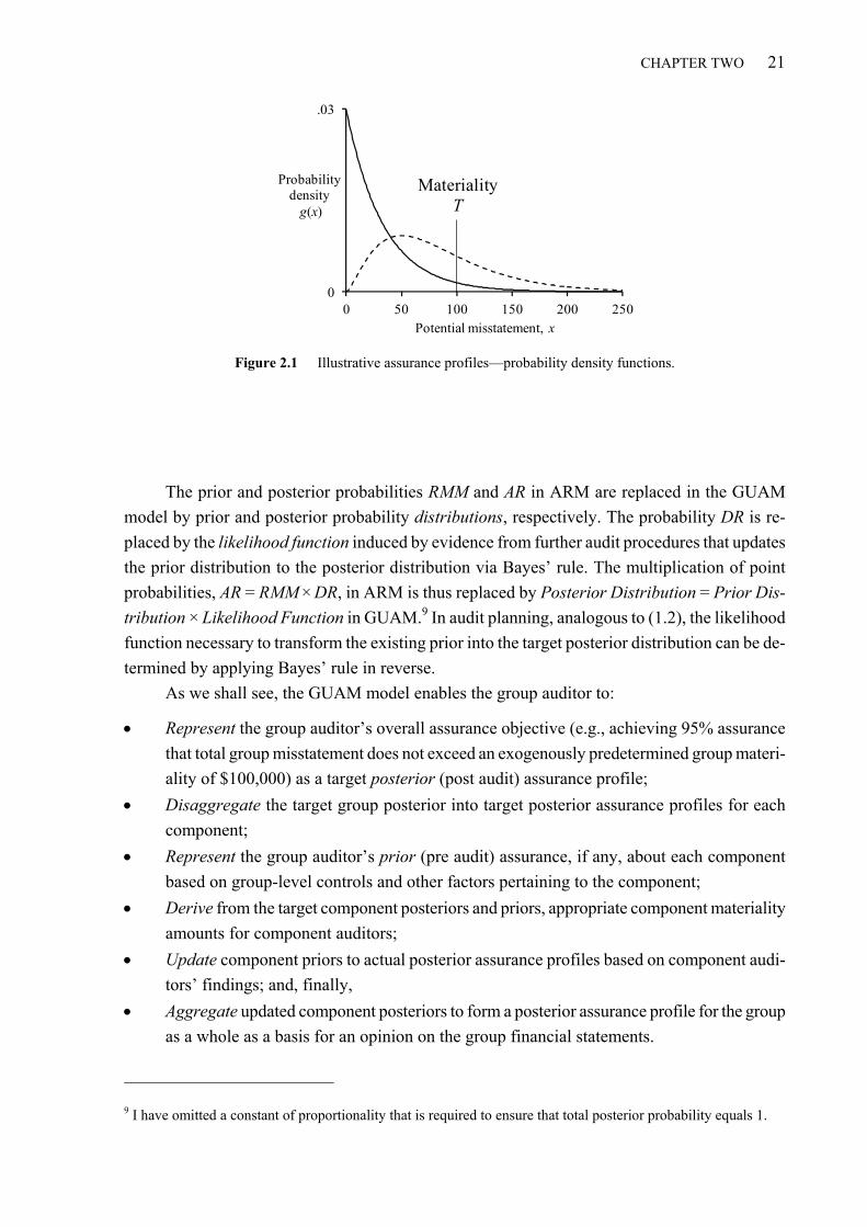
CHAPTER TWO 21
Figure 2.1 Illustrative assurance profiles—probability density functions.
The prior and posterior probabilities RMM and AR in ARM are replaced in the GUAM
model by prior and posterior probability distributions, respectively. The probability DR is re-
placed by the likelihood function induced by evidence from further audit procedures that updates
the prior distribution to the posterior distribution via Bayes’ rule. The multiplication of point
probabilities, AR = RMM × DR, in ARM is thus replaced by Posterior Distribution = Prior Dis-
tribution × Likelihood Function in GUAM.9 In audit planning, analogous to (1.2), the likelihood
function necessary to transform the existing prior into the target posterior distribution can be de-
termined by applying Bayes’ rule in reverse.
As we shall see, the GUAM model enables the group auditor to:
Represent the group auditor’s overall assurance objective (e.g., achieving 95% assurance
that total group misstatement does not exceed an exogenously predetermined group materi-
ality of $100,000) as a target posterior (post audit) assurance profile;
Disaggregate the target group posterior into target posterior assurance profiles for each
component;
Represent the group auditor’s prior (pre audit) assurance, if any, about each component
based on group-level controls and other factors pertaining to the component;
Derive from the target component posteriors and priors, appropriate component materiality
amounts for component auditors;
Update component priors to actual posterior assurance profiles based on component audi-
tors’ findings; and, finally,
Aggregate updated component posteriors to form a posterior assurance profile for the group
as a whole as a basis for an opinion on the group financial statements.
9 I have omitted a constant of proportionality that is required to ensure that total posterior probability equals 1.
0
.03
0 50 100 150 200 250
Probability density
g(x)
Potential misstatement, x
MaterialityT

22 REPRESENTING, ACCUMULATING, AND AGGREGATING ASSURANCE
2.1.2 Most probable (modal) misstatement
The total area under a probability density function (assurance profile) is always 1, representing
total probability. The area between any two amounts on the x axis represents the probability (the
auditor’s degree of belief) that total misstatement will fall between those amounts. The x value at
which the assurance profile peaks (the point of maximum probability density) is the mode of the
distribution: it is the most probable misstatement.10 In the ISAs, this amount is known as project-
ed misstatement or the auditor’s best estimate of misstatement. The context in which those terms
are used in the ISAs relates to projections and estimates based on the results of audit samples. The
language used in the ISAs is derived from classical statistics where it is meaningless to say that a
value for total misstatement is the “most probable”: total misstatement is regarded as a fixed
(though unknown) amount that the auditor can estimate but cannot legitimately make probability
statements about. In Bayesian statistics, however, total misstatement is regarded as a random var-
iable and it makes perfect sense to describe a value of potential total misstatement as most proba-
ble. We will tend to use that term, which is more evocative than its blander synonym modal mis-
statement. As we shall see, in cases where prior assurance is ignored and substantive assurance is
derived from the results of audit samples, most probable misstatement is numerically equal to
projected misstatement.
2.2 Auditors as Bayesians
Leslie (1984, 104) describes the audit process conceptually as follows:
The audit can be described as a continuous process. In theory, the auditor commences this process with a con-tinuous distribution representing the prior probability of error based on his assessment of inherent risk and preventive controls. As each piece of evidence is obtained the auditor revises this distribution. If the evidence is favorable, the peak of the curve will move away from materiality, and the area of the curve beyond materi-ality will diminish. Conversely, if a piece of evidence is unfavorable, the peak will move toward materiality, and more of the area will be beyond that point. When all procedures have been completed, the final (posteri-or) distribution is the basis for the opinion given on the financial statements… If the distribution peaks to the left of materiality but the area to the right of materiality is too large, the risk would be too high to warrant an unqualified opinion even though a material error would not be likely. The auditor would not have obtained “reasonable assurance” that a material error did not exist.
In discussing Leslie’s paper, Kinney (1984, 131) says, “While there is little disagreement that au-
ditors tend to behave as if they are Bayesians, there is much disagreement as to how this should
be expressed in professional standards. There is a valid question of how much ‘theory’ should be
in professional standards. I do not believe that much more structure is likely to be forthcoming
from the ASB [the AICPA’s Auditing Standards Board].” He was right, and today’s recently
“clarified” statements are even less theoretically informative than those they replaced.
Many other scholars and practitioners agree that the audit process is essentially Bayesian
and that assurance should be represented by Bayesian models, for example, Felix (1974), Leslie 10 While some probability distributions have multiple modes, those that occur in auditing are invariably unimodal like those in Figure 2.1.

CHAPTER TWO 23
et al. (1979), Steele (1992), van Batenburg et al. (1994), Wille (2003), and Broeze (2006). Such
models can accommodate subjective inherent and control risk assessments (Kinney 1975; Bailey
1981), and are fully consistent with widely-used audit sampling techniques and analytical proce-
dures (Kinney 1979; Stringer and Stewart 1996; Stewart 2012). Auditing standards also suggest
that the audit process is essentially Bayesian. For example, ISA 330, paragraph A60 explains,
“An audit of financial statements is a cumulative and iterative process. As the auditor performs
planned audit procedures, the audit evidence obtained may cause the auditor to modify the nature,
timing or extent of other planned audit procedures.”
Strangely, while auditing is an almost ideal field for the application of Bayesian methods,
the fact is that very little progress has been made. Writing from the perspective of 1984, Leslie
added the following optimistic comment to those quoted above: “In the past, the theoretically cor-
rect model has been virtually impossible to use in practice. Now with the increasing use of com-
puterized audit decision aids, it is becoming increasingly more feasible. It is not too difficult to
predict that within the foreseeable future such complex models will be an integral part of the au-
dit.” To which Kinney added, “Increasing competition and the micro computer are making opera-
tional many of the models that we have discussed at this conference for the last ten years… Field
workers now have the computing power necessary to do sophisticated audit planning and evi-
dence integration. We scholars can no longer avoid these issues by using the excuse of computa-
tional impracticality.” Alas, nearly three decades later, the integration of such models has not
happened despite the ready availability of computational power unimaginable three decades earli-
er and despite an enormous surge of interest in Bayesian methods in other application areas since
the early 1990s (The Economist 2000; O’Hagan et al. 2006).
In my opinion, one reason for this lack of progress is a general decline in interest in the ap-
plication of quantitative, probabilistic and statistical methods in auditing that began in the 1980s.
Accounting firms reduced basic audit research in this area as they focused on the development of
new services. Academic research into and teaching of such methods declined as a consequence,
leading to a further decline in practitioner awareness and proficiency. The methods were also per-
ceived as difficult to apply and meld with professional judgment, and the cost-benefit of training
auditors to be proficient in them was questioned. Interest, proficiency, and academic engagement
declined. In the aftermath of accounting scandals and audit failures in the early 2000s and the im-
position of new regulatory regimes, there has been a glimmer of reawakening interest in auditing
methodology; and, of course, the technological environment is rich with opportunities for im-
provement.
A reason for the general lack of enthusiasm for statistical methods can be found in what I
believe to be misplaced emphasis on classical rather than Bayesian statistics in auditing literature
and teaching. In the preface to his book, Lee (2012) explains the intuitive appeal of Bayesian sta-
tistics:
When I first learned a little statistics, I felt confused, and others I spoke to confessed that they had similar feelings… because I found it difficult to follow the logic by which inferences were arrived at from data. It sounded as if the statement that a null hypothesis was rejected at the 5% level meant that there was only a 5% chance of that hypothesis being true, and yet the books warned me that this was not a permissible interpreta-
24 REPRESENTING, ACCUMULATING, AND AGGREGATING ASSURANCE
tion. Similarly, the statement that a 95% confidence interval for an unknown parameter ran from -2 to +2 sounded as if the parameter lay in that interval with 95% probability and yet I was warned that all I could say was that if I carried out similar procedures time after time then the unknown parameters would lie in the con-fidence intervals I constructed 95% of the time. It appeared that the books I looked at were not answering the questions that would naturally occur to a beginner, and that instead they answered some rather recondite ques-tions which no-one was likely to want to ask. …I was told that there was another theory of statistical inference, based ultimately on the work of the Rev. Thomas Bayes, a Presbyterian minister who lived from 1702 to 1761… However, I was warned that there was something not quite proper about this theory, because it depended on your personal beliefs and so was not ob-jective. More precisely, it depended on taking some expression of your beliefs about an unknown quantity be-fore the data was available (your “prior probabilities”) and modifying them in the light of the data (via the so-called “likelihood function”) to arrive at your “posterior probabilities” using the formulation that “posterior is proportional to prior times likelihood”. The standard, or “classical”, theory of statistical inference, on the oth-er hand, was said to be objective, because it does not refer to anything corresponding to the Bayesian notion of “prior beliefs”. Of course, the fact that in this theory you sometimes looked for a 5% significance test and sometimes for a 0.1% significance test, depending on what you thought about the different situations in-volved, was said to be quite a different matter. I went on to discover that this theory could lead to the sorts of conclusions that I had naïvely expected to get from statistics when I first learned about it. Indeed, [books on Bayesian statistics] showed that if the statis-tician had “personal probabilities” that were of a certain conventional type then conclusions very like those in the elementary books I had first looked at could be arrived at, with the difference that a 95% confidence inter-val really did mean an interval in which the statistician was justified in thinking that there was a 95% proba-bility of finding the unknown parameter…
Lee’s commentary casts light on why statistical techniques are not well understood or popu-
lar in the auditing profession. As discussed in Section 1.3, auditing standards require auditors to
achieve a reasonable level of assurance (95%), that total misstatement does not exceed materiali-
ty, and to reduce audit risk to an appropriately low level (5%). These probabilities are clearly
meant to represent degrees of professional belief—which is entirely appropriate in auditing,
where professional judgment is paramount. While achieving such Bayesian-probabilistic conclu-
sions is beyond the reach of classical statistics, it is classical statistics that is nevertheless the ba-
sis of most audit sampling texts (e.g., AICPA 2012) and it is what auditors are taught. There is a
disconnect. Auditors want to conclude that there is a 5% risk that total misstatement exceeds ma-
teriality. Instead, they are taught to conclude that there is a 5% risk of incorrect acceptance of the
hypothesis that total misstatement does not exceed materiality—a conclusion that is rather less
satisfying and does not appear to be what auditing standards are really asking for.
Matters get more confusing when (prior) risk of material misstatement enters the picture
because that is essentially a subjective probability in the spirit of Bayes. However, instead of
Bayes’ rule, which explains how prior probabilities are revised for sample evidence, we have the
ARM which multiplies subjectively determined RMM by the risk of incorrect acceptance of an
hypothesis, DR, to arrive at an incoherent hybrid overall audit risk, AR.
2.3 A brief primer on gamma distributions
The GUAM model represents priors, posteriors and likelihoods with gamma probability distribu-
tions. The gamma family provides a rich variety of distribution shapes that tend to be intuitively
appealing as models of judgmental assurance—shapes ranging from exponential to almost bell-

CHAPTER TWO 25
shaped. For example, if there is no indication of misstatement, then it is reasonable to represent
that state with an assurance profile that peaks at zero and where the probability associated with
increasingly large amounts of misstatement declines exponentially—in other words with an ex-
ponential distribution such as that depicted in Figure 2.1. As we shall see, it is precisely an expo-
nential distribution that is induced if the only audit assurance is derived from a misstatement-free
monetary unit sample (MUS). Where there is evidence of misstatement, it is reasonable to repre-
sent that state with an assurance profile that peaks at most probable misstatement. Again, MUS
samples containing misstatements induce gamma distributions that peak at most probable mis-
statement.
Gamma distributions have two parameters: a shape parameter > 0 that determines the
basic shape of the distribution, and a scale parameter > 0 that for any given shape determines
the diffusion or spread of X. Gamma distributions with = 1, 2, and 3 and the same scale param-
eter are depicted in Figure 2.2. The figure depicts the probability density function (PDF), which
best displays the overall shape and diffusion of the distribution, as well as the cumulative distri-
bution function (CDF), which is more useful for reading probabilities. If were smaller, the PDFs
would be less diffuse (more concentrated and peaked), and if were larger, the PDFs would be
more diffuse (more spread out and flatter). For any given value x, the CDF gives the probability
that random variable X will be less than or equal to x, that is, Pr(X x). This is equal to the rela-
tive area under the PDF to the left of x. Conversely, for any given probability P on the vertical
axis, the CDF can be used to find the x value that represents the P-th percentile (50% is depicted
in the figure).
Exponential ( = 1) distributions arise in auditing when there is no evidence of misstate-
ment and therefore most probable misstatement is zero. Distributions with > 1 arise when there
PDF = 1, exponential = 2 = 3
Den
sity
, g (x
)
CDF = 1, exponential = 2 = 3
Pro
babi
lity,
G (x
)
Potential misstatement, x Potential misstatement, x Potential misstatement, x
Figure 2.2 Gamma probability density functions g (x) (top) and cumulative distribution functions G (x) (bot-tom), various shapes () and scale parameter = 1.
0
.5
1.0
0
.5
1.0

26 REPRESENTING, ACCUMULATING, AND AGGREGATING ASSURANCE
is evidence of misstatement and the distribution peaks at the most probable total misstatement.
They also arise in group audits where multiple component distributions are aggregated to form
the distribution for a group—even if there is no evidence of misstatement in any component. Dis-
tributions with < 1 (not illustrated in Figure 2.2) are more skewed and peaked at zero than the
exponential distribution. They arise in certain special circumstances such as the presence of
strong group-wide controls as discussed and illustrated in Chapter 7.
2.3.1 The gamma distribution
Random variable X has a gamma distribution with parameters and , denoted by X ~ g (, ), if
its PDF is
1 /( / )
( ; , ) for 0 and , 0( )
xx eg x x
, (2.1)
where 1
0( ) a ta t e dt
(Johnson et al. 1994, 337). The gamma function Γ has the recursive
property Γ() = ( − 1) Γ( − 1), and Γ(1) = 1. Therefore, for positive integer values of
( ) ( 1)( 2) 2 1 ( 1)! (2.2)
Values of the PDF can be calculated in Excel as
( ; , ) GammaDist( , , , FALSE)g x x cumulative ,
which was used to plot the PDFs in Figure 2.2.
Important properties of gamma-distributed X include its mode,
( 1) , 1
Mode( )0, 1,
X
(2.3)
its expected value (or mean),
( )E X , (2.4)
its variance,
2Var( )X , (2.5)
and its standard deviation,
( )X .
From (2.4) and (2.5) it follows that the parameters of the gamma distribution can be expressed in
terms of the expected value and variance,
2[ ( )] Var( )
and Var( ) ( )
E X X
X E X . (2.6)

CHAPTER TWO 27
As suggested by Figure 2.2, the gamma distribution becomes more bell-shaped as the pa-
rameter increases. In fact it tends to the normal distribution as increases (Johnson et al. 1994,
340), so that for large ,
( , ) ( , )g Normal . (2.7)
2.3.2 Cumulative distribution
The gamma CDF
0
( ; , ) ( ; , )x
G x g t dt
gives the probability that the value of X does not exceed x, that is, G(x; , ) = Pr(X x). Graph-
ically, it is the area under the PDF g(x; , ) between 0 and x. There is no general closed-form
formula for the gamma CDF but its values can be calculated in Excel as
( ; , ) GammaDist( , , , TRUE)G x x cumulative ,
which was used to plot the CDFs in Figure 2.2. Because is a scale parameter,
( ; , ) ( / ; ,1)G x G x . (2.8)
In words, the probability that a random variable distributed as gamma with scale will not ex-
ceed x is equal to the probability that a random variable distributed as gamma with scale 1 will
not exceed x / .
2.3.3 Percentile function
The percentile function Q(P; , ) is the inverse of G(x; , ). If G(x; , ) = P < 1, then x =
Q(P; , ) is the 100P-th percentile of X. Visually, percentile functions are simply CDF functions
(such as those in Figure 2.2) in reverse so that for each probability P on the vertical axis the func-
tion finds the corresponding x value on the horizontal axis—which is the value of x such that the
relative area to the left of it under the PDF is P. Because is a scale parameter,
( ; , ) ( ; ,1)Q P Q P ,
which for conciseness we write as QP(). In words, the 100P-th percentile of a gamma distribu-
tion with scale is equal to times the 100P-th percentile of a gamma distribution with scale 1.
For example, Q.95() is the 95th percentile of a random variable X distributed as g(, ).
There is no general closed-form formula for gamma percentiles but they can be calculated
in Excel as
( ) GammaInv( , , )pQ P . (2.9)

28 REPRESENTING, ACCUMULATING, AND AGGREGATING ASSURANCE
Because a bug in Excel (at least in Excel 2007 and earlier versions) causes (2.9) to give incorrect
results for large , it is safer to use the function as
( ) GammaInv( , ,1)pQ P .11 (2.10)
For some analytical and computational purposes it is useful to have an explicit functional
approximation to the percentile function. For ≥ 1 and P ≥ 50% a good approximation is
221 1
( ) 4 1 14 12P P PQ a u a u , (2.11)
where uP is the 100P-th percentile of the standard normal distribution (Johnson et al. 1994, equa-
tion 18.25).12 The standard normal percentile can be calculated in Excel as
NormSInv( )Pu P .
From (2.7), for large enough we can also use the normal percentile as an approximation
( )P PQ u . (2.12)
If the value Q of the 100P-th percentile is known and Q ≥ −ln(1 − P), then (2.11) can be used to
solve explicitly for as
2
21 1( 1)
12 2 4P
P
uQ u
. (2.13)
2.3.4 The exponential distribution
Peaking at zero and declining monotonically as X increases, exponential ( = 1) distributions
have the right overall shape for representing assurance where there is no indication of misstate-
ment. Section 3.3 shows that they are even implicit in the ARM in the sense that ARM works cor-
rectly if and only if RMM and DR are probabilities from exponential distributions. Further, as ex-
plained in Section 3.5, the exponential distribution is generally the best representation of assur-
ance when there is no indication of misstatement—a consequence of its status as a maximum en-
tropy distribution.
11 The function GammaInv(P, , ), which should increase for increasing , gets stuck at 10,000,000 once the function reaches that value. This is a problem in auditing applications where values of 10,000,000 and greater are common. The problem occurs with Excel 2007 and earlier and I have not tested it with later versions. Fortu-nately, the formulation in (2.10) is an easy workaround for any . 12 I compared this approximation with the GammaInv function in Excel 2007 for ≥ 1 and P = .95. The greatest relative error is at = 1 where it is 1/1000. The error decreases very rapidly to 1/10000 at about = 2 and tends asymptotically to zero after that. The approximation is particularly good for P .95, but is in any case acceptable for any P ≥ .5 for the purposes for which it is used in this thesis. Due to a bug in Excel (at least in Excel 2003 and 2007), (2.10) can result in #NUM! errors for very large values of , starting at about = 380. Other soft-ware or an approximation such as (2.11) should be used for such large values.

CHAPTER TWO 29
For exponential distributions,
2Mode( ) 0, ( ) , and Var( )X E X X ,
and the probability functions have simple closed forms. The PDF is
/1( ;1, ) xg x e
, (2.14)
the CDF is
/ /
0
1( ;1, ) 1
x
t xG x e dt e
,
and the percentile function is
(1) ln(1 )Px Q P . (2.15)
The factor QP(1) in (2.15) occurs frequently in this thesis and also in the sampling literature
where it is known as a reliability factor or R factor and denoted RP. Thus, R factor RP is defined
as
(1) ln(1 )P PR Q P . (2.16)
Some commonly encountered levels of assurance and associated R factors are listed in Table 2.1.
From (2.15) and (2.16), the 100P-th percentile of an exponential distribution g(x; 1, ) is
RP. Conversely, if the 100P-th percentile is known to be some amount QP and it is known that
the probability distribution is exponential, then RP = QP and the specific distribution is uniquely
identified as g(x; , ), where = QP / RP. In audit planning, the percentile is typically materiality,
T, in which case the assurance level P is associated with an exponential distribution
( ;1, ), whereP
Tg x
R . (2.17)
For example, if the auditor has 95% assurance that total misstatement does not exceed T, then T =
R.95 = 3.0 and the exponential assurance profile is g(x; 1, T / 3.0).
Where RMM is quantified as a single point probability it is a straightforward matter to con-
vert that representation to an assurance profile. Table 2.2 illustrates how that might be done in
practice. It starts with verbal descriptions of audit assurance ranging from “Negligible” through
Table 2.1 Assurance levels and reliability factors
Assurance, P R factor
95% 3.0 90% 2.3 86% 2.0 70% 1.2 63% 1.0 50% 0.7

30 REPRESENTING, ACCUMULATING, AND AGGREGATING ASSURANCE
“Very High” and to these are assigned quantitative levels of assurance ranging from 0% to 90%.
Accordingly, RMM ranges from 100% to 10%. These quantifications are based on RMM percent-
ages given as examples in AU 350 (AICPA 2006b). The verbal descriptions are mine, though
quite typical of those used in practice (Martinov and Roebuck 1998).13 If the auditor’s prior as-
surance is P that total misstatement does not exceed T, it can be equivalently stated that the risk
of material misstatement is RMM = 1 – P or that T is the 100P-th percentile of the appropriate pri-
or assurance profile. From (2.17) it follows that the prior assurance profile is g(x; 1, T / RP). For
example, “moderate” assurance is represented by g(x; 1, T / 0.7).
We can represent the target posterior assurance similarly. If AR = 5% then P = 1 − AR =
95%; from Table 2.1, R.95 = 3.0; and the appropriate posterior assurance profile is g(x; 1, T / 3.0).
Finally, DR = AR / RMM = 5% / 50% = 10% and P = 1 − DR = 90%. Therefore, from Table 2.1,
R.90 = 2.3 and the appropriate likelihood function is g(x; 1, T / 2.3). The exponential prior, likeli-
hood, and posterior just described are depicted in Figure 2.3.
Table 2.2 Examples of prior assurance
Description of prior assurance
Assurance, P RMM =
1 − P RP =
−ln(RMM) Implied prior
Negligible 0% 100% 0.0 Negligible Very Low 10% 90% 0.1 g(x; 1, T / 0.1)
Low 30% 70% 0.4 g(x; 1, T / 0.4) Moderate 50% 50% 0.7 g(x; 1, T / 0.7)
High 70% 30% 1.2 g(x; 1, T / 1.2) Very High 90% 10% 2.3 g(x; 1, T / 2.3)
Figure 2.3 Exponential prior, likelihood and posterior distributions g(x; 1, 100 / RP).
13 Although it is often easier for auditors to assign verbal descriptors rather than precise probabilities to risks, if a risk is used in subsequent calculations it is necessary to assign a quantitative value to it “behind the scenes”.
0
.03
0 50 100 150 200 250
g(x)
Potential misstatement, x
Prior: R.50 = 0.7Likelihood: R.90 = 2.3
Posterior: R.95 = 3.0
T = 100 is:50th percentile for Prior90th percentile for Likelihood95th percentile for Posterior

CHAPTER TWO 31
2.4 Using Bayes’ rule to evaluate and plan posterior assurance
In the Bayesian paradigm, further audit procedures (that is, those performed after prior assurance
has been assessed) induce a likelihood function, which is essentially the probability distribution of
X given only the new evidence and ignoring prior assurance.
Bayes’ rule governs how likelihood functions update prior assurance profiles into posteri-
ors. In a fairly general Bayesian setting, one has evidence κ and wishes to infer about a parameter
x. If the necessary functions of x exist and are continuous then Bayes’ rule can be written as
( ) ( | )
( | )( ) ( | )
f x f xf x
f x f x dx
(2.18)
(O’Hagan and Forster 2004, 1.9). Here f (x) is the prior distribution of X, and f (κ | x) is the likeli-
hood function. The likelihood function is formally the same as the distribution of κ given fixed x,
except that it is interpreted as a function of x given fixed observed κ. The product of the prior dis-
tribution and the likelihood function is divided by a normalizing constant to ensure that its total
integral is 1 and the result is the posterior distribution of X given evidence κ. O’Hagan and For-
ster (2004, 1.10) provide a nicely intuitive interpretation of Bayes’ rule:
The prior density f (x) represents the prior information about x. We then observe the data κ and Bayes’ theo-rem constructs the posterior density f (x | κ) as proportional to the product of the prior density and the likeli-hood f (κ | x), thereby combining the two sources of information. Posterior density for particular values of x will be low if they have low prior density or low likelihood, so they are essentially discounted by one or other source of information. Appreciable posterior density will exist at values of x for which neither prior density or likelihood is very low. If there are values that are well sup-ported by both information sources, i.e. having high prior density and high likelihood, then these values will also have high posterior density. [Notation modified for consistency.]
Note that the likelihood function, a function of x, is not a probability distribution unless its
total integral equals 1. However, in Bayesian theory two likelihood functions are equivalent if one
is a scalar multiple of the other (Wille 2003, 48; O’Hagan and Forster 2004, 3.2). We can there-
fore standardize the likelihood function f (κ | x) by dividing it by ( | )f x dx
(assuming the inte-
gral exists) so that the quotient has total probability 1 and can be regarded as the probability dis-
tribution of X given only evidence κ.14 This is allowable because the scalar multiplier appears in
both the numerator and denominator in (2.18) and has no effect on the posterior probability. We
will use the term likelihood distribution for such a standardized likelihood function.
2.4.1 Bayes’ rule applied to gamma distributions
Assuming that further audit procedures induce a gamma likelihood distribution with shape ≥ 1, it
will be convenient to denote it g(x; 1 + κ, B) so that the mode (most probable misstatement) is
14 While in general it cannot be taken for granted that the integral converges (Raiffa and Schlaifer 2000, 48), it does for the likelihoods we will consider.

32 REPRESENTING, ACCUMULATING, AND AGGREGATING ASSURANCE
[(1+ κ) − 1] B = κB.15 Applying such a likelihood to a prior g(x; , ) via Bayes’ rule gives the pos-
terior gamma distribution
0
( ; , ) ( ;1 , )( ; , )
( ; , ) ( ;1 , )
g x g x Bg x
g x g x B dx
, (2.19)
where
1
and1/ 1/ B
. (2.20)
This result may be derived by substituting the appropriate gamma density functions per equation
(2.1) into the right-hand side of Bayes’ rule (2.19) and performing some algebraic manipulation.
Taking the numerator on the right-hand side of (2.19) we have
1 / /
( ) 1 (1/ 1/ )1
1 /
1
( / ) ( / )( ; , ) ( ;1 , )
( ) (1 )
1
( ) (1 )
( ) ( ) ( / ),
( ) (1 ) ( )
x x B
x B
x
x e x B eg x g x B
B
x eB
x e
B
(2.21)
where ʹ and ʹ are as defined in (2.20). That is,
( ; , ) ( ;1 , ) ( ; , )g x g x B Kg x ,
where K is the bracketed constant in the last line of (2.21). In equation (2.19), therefore,
0 0
( ; , ) ( ;1 , ) ( ; , ) ( ; , )( ; , )
1( ; , ) ( ;1 , ) ( ; , )
g x g x B Kg x Kg xg x
Kg x g x B dx K g x dx
.
In cases like this, where the posterior distribution belongs to the same family as the prior,
the prior and posterior are called conjugate distributions, and the prior is called a conjugate prior
for the likelihood (Raiffa and Schlaifer 2000). A conjugate prior is an algebraic convenience, giv-
ing a closed-form expression for the posterior (and avoiding what might otherwise entail a diffi-
cult numerical integration). Further, conjugate priors aid intuition, by more transparently showing
how a likelihood function updates a distribution.16
15 As we shall see in Section 3.2, a MUS sample with k misstatements induces the likelihood distribution g(x;1 + k, B), where B is the average sampling interval. The mode k B is most probable misstatement. If the sam-ple is misstatement free (k = 0), then the induced likelihood is the exponential distribution g(x;1, B) with mode zero. The results of non-MUS procedures can ordinarily be evaluated as evidentially equivalent MUS samples (Teitlebaum 1973; Smith 1976; Leslie et al. 1979; Steele 1992), though not necessarily with the same rigor, and can be deemed to induce standardized likelihood distributions of the form g(x;1 + κ, B). 16 The description of conjugate distributions in this paragraph has been adapted from the entry for “conjugate prior” in Wikipedia.

CHAPTER TWO 33
Note that when the prior and likelihood are exponentials, = 1, κ = 0 and, from (2.20), ʹ =
1 + 0 = 1, so the posterior is also an exponential distribution. In auditing terms, if there is no prior
indication of misstatement and further audit procedures reveal no misstatement, then a posteriori
there is also no indication of misstatement. The mathematical outcome, per (2.20), is an exponen-
tial posterior with a scale parameter smaller than that of the prior. That is, the posterior is simply
a “tighter”, less diffuse exponential assurance profile with greater density in the neighborhood of
the zero mode.
Analogous to ARM equation (1.2), Bayes’ rule can be applied in reverse for audit planning
purposes. If the auditor desires a posterior assurance profile g(x; ʹ, ʹ) and starts with a prior
g(x; , ), where ʹ < and ʹ ≥ , then from (2.20) the required likelihood distribution is
g(x; 1 + κ, B), where
1
and1/ 1/
B
. (2.22)
For example, for the prior and posterior distributions illustrated in Figure 2.3, we can use
Bayes’ rule to directly determine the target likelihood distribution. The prior is g(x; 1, T / 0.7) and
the target posterior is g(x; 1, T / 3.0), so from (2.22)
1
1 1 0 and1/ ( / 3.0) 1/ ( / 0.7) 3.0 0.7 2.3
T TB
T T
and the target likelihood is g(x; 1, T / 2.3).17 Note that as long as we stick with exponential distri-
butions, the ARM and GUAM representations of assurance are essentially interchangeable. In
ARM we have 5% = 50% × 10%, while in GUAM, Bayes’ rule leads to R.95 = R.5 + R.9, or 3.0 =
0.7 + 2.3. Both cases lead to AR = 5%. The relationship between exponential distributions and
ARM is explored in Section 3.3. In Section 3.4 we will see that when priors or likelihoods are not
exponential distributions the ARM tends to understate the true audit risk, which requires Bayes’
rule for its correct calculation.
2.4.2 Negligible priors
When auditors assess RMM they take into account inherent risks and the quality of internal con-
trols. If they believe that there is significant inherent risk or they find that internal controls are
poor they commonly (and conservatively) assume that the risk of material misstatement is 100%,
with the result that all the auditor’s assurance must come from further audit procedures and audit
risk equals detection risk (AR = 100% × DR = DR). In the Bayesian paradigm, having absolutely
no prior assurance (RMM = 100%) is a conservative, theoretical limit and it is necessary for tech-
nical reasons to instead think of the auditor as having negligible prior assurance.
17 As we shall see in Section 3.2 this likelihood function can be achieved with a misstatement-free monetary unit sample (MUS) selected using an average sampling interval of B = T / 2.3.

34 REPRESENTING, ACCUMULATING, AND AGGREGATING ASSURANCE
Operationally, we will treat a negligible prior as an exponential distribution g(x; 1, ) with a
scale parameter so large relative to T that 1 / can be regarded as effectively zero in (2.20) and
(2.22), and, consequently, B = ʹ and g(x; 1, ʹ) = g(x; 1, B). The net effect is that essentially all the
auditor’s assurance comes from further audit procedures and thus a negligible prior achieves the
same as setting RMM = 100%.
2.5 Aggregating assurance across components
We have seen how assurance for a single entity can be represented by the probability distribution
g(x; , ) of a random variable X representing total misstatement. For group audits there are mul-
tiple components by definition and the problem is to determine the overall assurance profile for
the group as a whole based on the component assurance profiles. This section describes how
component gamma distributions aggregate to an overall group distribution that is approximately a
gamma distribution. (As indicated in Section 1.3.2, ARM is strictly a single entity model and has
no construct for aggregating assurance across multiple entities.)
2.5.1 Approximating the group assurance profile
If there are N components with random variables Xi ~ g(i, i), i = 1, 2, …, N, the group auditor is
interested in the group assurance profile—the probability distribution of the aggregate random
variable1
N
iiX
. If the Xi are stochastically independent (something we will assume), the proba-
bility distribution of that aggregate random variable is the convolution of the N component proba-
bility distributions (DeGroot and Schervish 2002, 172).
In general, the convolution of a set of gamma distributions g(xi; i, i) is complicated, and
difficult to compute and work with analytically. However, the convolution can be approximated
by another gamma distribution with the correct expected value and variance (Stewart et al. 2007).
From (2.4), (2.5) and well known properties of the sum of independent random variables, the ex-
pected value and variance of the true convolution are
( ) andi i i iE X E X (2.23)
2Var Var( )i i i iX X . (2.24)
The approximating gamma distribution is therefore ( ; , )ig x , where, from (2.6),
2 2
2and
Var
i i i
i ii
E X
X
(2.25)
2Var i i i i i
i ii
X
E X
. (2.26)

CHAPTER TWO 35
The approximation is discussed further in Section 6.1. In the special case where the i’s are all
equal to , the convolution is exactly ( ; , )ig x with i (DeGroot and Schervish 2002,
298).
If we limit ourselves to N exponential distributions g(xi; 1, i) then i = 1 and
2
2
i
i
, (2.27)
2i i
i
. (2.28)
If the i’s all equal , then = N and the convolution further reduces to
~ ( , )iX g N . (2.29)
Note that, regardless of the i’s, N, with equality if and only if the i’s are equal.18
2.5.2 Determining overall group assurance: illustrative examples
Figure 2.4 depicts two identical exponential component assurance profiles g(xi; 1, 100 / 3.0), i = 1,
2, whose convolution per (2.29) results in the group assurance profile g(x1+x2; 2, 100 / 3.0). The
two component posterior profiles could be the result of instructing each component auditor to ap-
ply Ti = 100. The components’ 95th percentiles are Q.95(1) = (100 / 3.0) × 3.0 = 100 and the group
95th percentile is Q.95(2) = (100 / 3.0) × 4.74 = 158. Because the latter exceeds T = 100, the com-
ponent assurance profiles depicted in Figure 2.4 do not meet the group auditor’s assurance objec-
tive—there is only 80% assurance that total misstatement does not exceed T = 100, that is,
Pr(X1 + X2 100) = G(100; 2, 100 / 3.0) = .8.
In contrast, Figure 2.5 shows that the group objective is achieved if target component scale
parameters are set to = 100 / 4.74. This target could be met by directing the component auditors
to achieve assurance profiles with 95th percentiles T1 = T2 = (100 / 4.74) × 3.0 = 63. This illustra-
tion is a simple example of the GUAM method for determining component materiality, which is
described more fully in Chapter 4.
It may appear counter-intuitive that component assurance profiles with modal (most proba-
ble) misstatement of zero should aggregate to a group profile with mode > 0. The analogy of a
portfolio of insurance policies may help build intuition: while the modal claim for each individual
policy in a particular year might be zero, the modal claim for a portfolio comprised of many such
policies would be greater than zero. 18 From the Cauchy-Schwarz inequality, 2 2 2
i i i i . Because i = 1, therefore 2i N ,
2 2i iN , and from (2.27),
2
2
i
i
N
. Also from Cauchy-Schwarz, = N if and only if the
i’s are all equal.

36 REPRESENTING, ACCUMULATING, AND AGGREGATING ASSURANCE
Component 1 g(x1; 1, 100 / 3.0)
Component 2 g(x2; 1, 100 / 3.0)
Group
g(x1 + x2; 2, 100 / 3.0)
Aggregateto
Conclude
Figure 2.4 Only 80% group assurance achieved on aggregation.
Component 1 g(x1; 1, 100 / 4.74) = g(x1; 1, 63 / 3.0)
Component 2 g(x2; 1, 100 / 4.74) = g(x2; 1, 63 / 3.0)
Group
g(x1 + x2; 2, 100 / 4.74) = g(x1 + x2; 2, 63 / 3.0)
Aggregateto
Conclude
Figure 2.5 Target 95% group assurance achieved on aggregation.
2.5.3 Aggregation in a multilevel group
Groups often have a multilevel inverted-tree structure with ultimate components as the leaves.
This is illustrated in Figure 2.6 where there are seven ultimate components (shown as shaded
boxes) organized hierarchically in three levels.
Mathematically, it makes no difference whether the group assurance profile is formed by
directly aggregating the ultimate end components or by aggregating stepwise from the bottom up,
first into subgroups and then ultimately into the top level group; and the order of aggregation is
also irrelevant. This is because convolutions are commutative and associative, properties that fol-
low directly from the fact that sums of random variables are also commutative and associative
0
.05
0 50 100 150 200
g(x1)
x1
Q.95 = 100
0
.05
0 50 100 150 200
g(x2)
x2
Q.95 = 100
0
.05
0 50 100 150 200
g(x)
x = x1 + x2
Q.95 = 158
Q.80 = 100
0
.05
0 50 100 150 200
g(x1)
x1
T1 = Q.95 = 63
0
.05
0 50 100 150 200
g(x2)
x2
T2 = Q.95 = 63
0
.05
0 50 100 150 200
g(x)
x = x1 + x2
T = Q.95 = 100

CHAPTER TWO 37
(Feller 1971, 7). That is, if f1 and f2 are density functions and their convolution is denoted by
1 2f f , then
1 2 2 1f f f f
(commutativity), and if f3 is a third density function then
1 2 3 1 2 3( ) ( )f f f f f f
(associativity). These commutative and associative properties of convolutions apply also to the
approximate convolution of gamma distributions explained in Section 2.5.1.
Figure 2.6 Multilevel group with ultimate components shaded (3 levels, 7 components).


39
CHAPTER 3 Gamma Distributions in Auditing
This chapter expands on the relevance of gamma distributions to auditing. It describes how audi-
tors’ subjective assurance can be represented by gamma distributions as well as how monetary
unit sampling (MUS) induces a gamma distribution model of assurance. It demonstrates how
gamma distributions ensure that the GUAM model is a true generalization of ARM, providing
correct results where ARM does not but agreeing with ARM where it does. Specifically, it shows
that ARM works correctly if and only if its probabilities come from exponential distributions. A
widely used table from the AICPA is used to illustrate how ARM understates audit risk. In a more
theoretical vein, the exponential distribution’s status as a maximum entropy distribution is used to
argue that, in the absence of indications of misstatement, exponential distributions ordinarily pro-
vide the best representation of audit assurance. After summarizing the reasons why gamma distri-
butions are the basis of the GUAM model, the chapter closes by outlining an alternative approach
using beta distributions.
This chapter may be skipped on a first reading although the MUS sample size formula de-
rived in Section 3.2 is used in later chapters.
3.1 Establishing prior and target posterior assurance profiles
Auditors get assurance from many sources. These include what they know about the inherent na-
ture of the business; their understanding of and tests of the operating effectiveness of internal
controls; informal gut-feel coherence checks in which they consider whether numbers and disclo-
sures “make sense”; formal substantive analytical procedures of various kinds, including statisti-
cal regression tests; recalculations or proofs-in-total; exploratory data analysis, which may in-
volve exhaustive computerized tests of data files and the examination of summaries and graphical
depictions together with tests of outliers; and detailed tests of transactions or balances selected
statistically, subjectively, or according to calculated risk profiles.
Assurance profiles should represent the auditor’s professional judgment based on all
sources of evidence. While a prior can be specified directly by subjective but informed introspec-
tive professional judgment (O’Hagan and Forster 2004, 5.33), tables and decision-support soft-
ware can help the auditor form such judgments within guidelines endorsed by the auditor’s firm.
Tables such as Table 2.2 are commonly used directly in the field or indirectly as the foundation of

40 GAMMA DISTRIBUTIONS IN AUDITING
a firms’ own expression of audit assurance policy or guidelines. McCrae (1974, 202) describes
such a table-driven approach implemented by Haskins & Sells (now Deloitte) as far back as the
early 1960s.
Finding an assurance profile that approximately fits the auditor’s state of mind is a way to
express professional judgment in explicit tractable terms so that it can be combined with other
professional judgments in a logical fashion. Jeffrey (2004, 76) writes, “The most important ques-
tions in the theory of probability concern ways and means of constructing reasonably satisfactory
probability assignments to fit [the expert’s]… state of mind.” He compares it to “trying on
shoes”, and notes that, “For this, there is no overarching algorithm.” There is an extensive litera-
ture on the elicitation of experts’ probability judgments—see, for example, O’Hagan et al. (2006)
and Broeze (2006). However, this thesis takes as its starting point the presumption, implicit in
auditing standards, that the auditor can articulate prior assurance or, equivalently, RMM (ISA
200, paragraph A42), and we focus on the mechanics of representing it with a gamma-based as-
surance profile.
The gamma family of probability distributions provides shapes that are intuitively appealing
to auditors as models of their prior assurance. Leslie (1985, 158-159) provides a good discussion
of the audit process and illustrates it with curves that are clearly gamma-like, though they are not
specifically identified as such.
The beta family of probability distributions is an alternative to the gamma family that also
provides intuitive and appealing shapes for representing audit assurance. Just as the gamma is
conjugate to the Poisson distribution, which is generally used in monetary unit sampling for sub-
stantive testing (AICPA 2012), the beta is conjugate to the binomial distribution, which is gener-
ally used for attributes sampling in tests of internal control compliance (AICPA 2012). The be-
ta/binomial combination is preferred by some authors (e.g., Steele 1992; Wille 2003) who focus
on error rates rather than absolute amounts of misstatement. The beta distribution can also be
used to describe monetary misstatement. However, just as the Poisson is simpler to use than the
binomial when it comes to monetary unit sampling, the gamma distribution provides a simpler
description of monetary misstatement than the beta. Both provide intuitive representations of the
auditor’s judgmental assessment of potential misstatement that are ordinarily quite similar.19 The
beta distribution is described and compared with the gamma in Section 3.7.
In the context of prior elicitation, Wille stresses the necessity of the prior distribution in
Bayesian analysis and says, “The question that remains is how to make a proper assessment of
this prior. For most people, it is extremely difficult to express their knowledge into a number of
parameters of a probability distribution function. One solution to this prior elicitation problem is
to determine the value of parameters out of other characteristics of the distribution, like the mean,
variance or upper or lower bounds concerning the parameter of interest.” For examples of this
kind see Kadane and Wolfson (1998). Steele (1992, 64) says that since the formulation of a prior
19 Ordinarily, materiality and contemplated potential misstatement are small relative to the size of the population (e.g., less than 10 percent). As these amounts increase relative to the size of the population the beta distribution provides a better representation relative to the gamma.

CHAPTER THREE 41
can only be done approximately, “a practical approach is to have a selection of standard or tem-
plate priors available, and to pick the one which most nearly matches the actual situation.” He
adds, that such template priors, “should ideally be analytically tractable, being easy to program,
easy to interpret, easily described and rich in shapes so that there is a good chance of expressing
prior information”, and that “it would be convenient if they were a closed family, that is if the
prior is a member of a conjugate family then so is the posterior.” Raiffa and Schlaifer (2000, 44)
list similar desiderata.
3.1.1 Finding a gamma distribution to represent assurance
The approach illustrated here follows the advice of Steele, Raiffa and Schlaifer, and Wille cited
above using the gamma family of distributions. Since shape and scale parameters are not intui-
tively easy to specify directly, establishing an assurance profile is best done by articulating cer-
tain characteristics from which parameters can be derived. Perhaps the most intuitive method is
for the auditor to specify the mode and an upper percentile, say the 95th. The mode represents the
auditor’s judgment as to the most probable misstatement and the 95th percentile represents a
common upper limit, though any percentile will do. In MUS applications the mode is projected
misstatement and the 95th percentile is the 95% upper error limit. The following discussion shows
how to fit a gamma distribution with ≥ 1 where the auditor specifies the mode and a percentile.
If the auditor specifies that X is exponentially distributed (i.e., Mode(X) = 0) and that the
100P-th percentile is Q, then we know from (2.17) that the distribution is g(x; 1, ) with =
Q / RP. For example, if the auditor specifies that the 95th percentile is 100, then = 100 / R.95 =
100 / 3.0 and the distribution is g(x; 1, 100 / 3.0). Typically, the specified upper percentile will be
materiality T, however we denote it Q for generality.
If the auditor specifies that X is gamma distributed with Mode(X) = m > 0 and 100P-th per-
centile Q, then per (2.3) the assurance profile g(x; , ) being described has a mode of
( 1)m (3.1)
and a 100P-th percentile of
( )PQ Q .
From this we get
( 1)
( )P
m
Q Q
and therefore
1
( )P
m
Q Q
, (3.2)

42 GAMMA DISTRIBUTIONS IN AUDITING
which can be solved for .20 Since > 1, it follows from (3.1) that
1
m
. (3.3)
For example, suppose that the auditor believes that the most probable total misstatement is
m = 30 and is 95% confident that total misstatement does not exceed Q = 100. The appropriate
assurance profile is the gamma distribution g(x; 2.8, 16.7) as depicted in Figure 3.1. Its parameters
can be determined as follows. The ratio of the mode to the 95th percentile is
30
0.3100
mr
Q .
From (3.2), therefore, the shape of the gamma distribution is the solution to the equation
.95
10.3
( )Q
,
which is = 2.8. This may be found using the Excel Goal Seek tool to solve
1
0.3GammaInv(95%, ,1)
.
The scale parameter comes from (3.3)
30
16.71 2.8 1
m
.
Figure 3.1 Gamma distribution with mode = 30 and 95th percentile = 100 is g(x; 2.8, 16.7).
20 A solution will only exist if the relationship between m, Q, and P is consistent with the gamma distribution. Because the gamma distribution it right skew, the 50th percentile (the median) is always greater than m. There-fore, solutions exist when Q > m and P ≥ 50%.
0
.02
0 20 40 60 80 100 120 140 160 180
g(x)
Potential misstatement, x
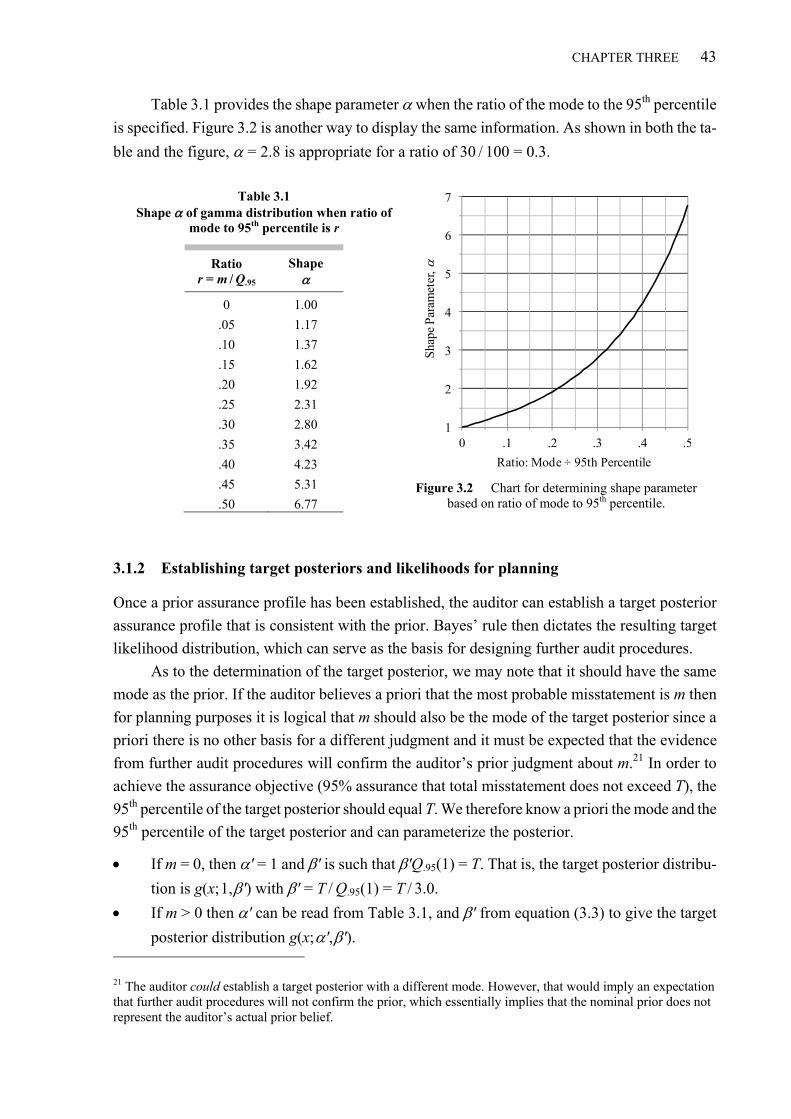
CHAPTER THREE 43
Table 3.1 provides the shape parameter when the ratio of the mode to the 95th percentile
is specified. Figure 3.2 is another way to display the same information. As shown in both the ta-
ble and the figure, = 2.8 is appropriate for a ratio of 30 / 100 = 0.3.
Table 3.1
Shape of gamma distribution when ratio of mode to 95th percentile is r
Ratio r = m / Q.95
Shape
0 1.00
.05 1.17
.10 1.37
.15 1.62
.20 1.92
.25 2.31
.30 2.80
.35 3.42
.40 4.23
.45 5.31
.50 6.77
Figure 3.2 Chart for determining shape parameter based on ratio of mode to 95th percentile.
3.1.2 Establishing target posteriors and likelihoods for planning
Once a prior assurance profile has been established, the auditor can establish a target posterior
assurance profile that is consistent with the prior. Bayes’ rule then dictates the resulting target
likelihood distribution, which can serve as the basis for designing further audit procedures.
As to the determination of the target posterior, we may note that it should have the same
mode as the prior. If the auditor believes a priori that the most probable misstatement is m then
for planning purposes it is logical that m should also be the mode of the target posterior since a
priori there is no other basis for a different judgment and it must be expected that the evidence
from further audit procedures will confirm the auditor’s prior judgment about m.21 In order to
achieve the assurance objective (95% assurance that total misstatement does not exceed T), the
95th percentile of the target posterior should equal T. We therefore know a priori the mode and the
95th percentile of the target posterior and can parameterize the posterior.
If m = 0, then ʹ = 1 and ʹ is such that ʹQ.95(1) = T. That is, the target posterior distribu-
tion is g(x; 1, ʹ) with ʹ = T / Q.95(1) = T / 3.0.
If m > 0 then ʹ can be read from Table 3.1, and ʹ from equation (3.3) to give the target
posterior distribution g(x; ʹ, ʹ). 21 The auditor could establish a target posterior with a different mode. However, that would imply an expectation that further audit procedures will not confirm the prior, which essentially implies that the nominal prior does not represent the auditor’s actual prior belief.
1
2
3
4
5
6
7
0 .1 .2 .3 .4 .5S
hape
Par
amet
er,
Ratio: Mode ÷ 95th Percentile

44 GAMMA DISTRIBUTIONS IN AUDITING
Given the prior and target posterior, the parameters of the target likelihood distribution are de-
rived from (2.22). These can be used to design the further audit procedures necessary to update
the prior to the target posterior. How this works in the case of MUS is explained in Section 3.2.
It may be noted that if the mode of the prior and target posterior distributions is m, then the
mode of the target likelihood distribution is also m. Because the prior and target posterior have
the same mode,
( 1) ( 1)m ;
and from (2.22),
1
and1/ 1/
B
.
If m = 0 then ʹ = = 1, κ = 0, and the mode of the likelihood is κB = 0. If m > 0 then the mode
of the likelihood distribution is
( )1/ 1/ ( 1) / ( 1) /
B B mm m
.
Therefore, in all cases the mode of the likelihood equals the mode of the prior and target posteri-
or. This is as it should be: the anticipated most probable misstatement based on further audit pro-
cedures alone should be the same as that anticipated a priori.
3.1.3 Approximation formula
Rather than solving for using an iterative method such as Excel Goal Seek or reading its value
from a table or chart, it is often more convenient to obtain the value of explicitly. Approxima-
tion formula (2.11) can be used for this provided P ≥ 50% (closer to 95% is better) and Q > m.
Setting
m
rQ
in (3.2), we have from (2.11),
221 1 1
( ) 4 1 ( 1)4 12P P PQ u u
r
.
Therefore, an approximate value of can be obtained by solving
224 1 ( 1) 1
4 12P P
r ru u . (3.4)
Let
4 1z .

CHAPTER THREE 45
Because we are seeking a gamma distribution with ≥ 1, therefore z ≥ 3 . We have
2 1
4 4
z , (3.5)
and from (3.4),
2
2 21( 1) 1
4 4 4 12P P
z r ru z u ,
which reduces to the quadratic equation in z
2 24 1(1 ) (2 ) 0, where 3
3 3P P P Pr z ru z C C ru r .
Solving for z gives the roots22
2 2
1 2
( ) (1 ) ( ) (1 )and
(1 ) (1 )P P P P P Pu r u r r C u r u r r C
z zr r
.
Noting that uP ≥ 0 for P ≥ 50% and that r < 1, we have CP > 0 and
2 2( ) ( ) (1 )P P P Pu r u r u r r C .
Therefore, z1 > 0 and z2 < 0. As noted earlier, we are only concerned with 3z , and so we may
ignore z2. Plugging z1 into equation (3.5) and simplifying, we get
22
2 23 (4 10) ( 1)13 3
2(1 ) 4
P P P
r ru r u u
r
. (3.6)
For example, for the distribution in Figure 3.1 we have r = 0.3 and u.95 = 1.645 giving
22
2 20.3 0.31.645 0.3 3 (4 1.645 10) (1.645 1)
13 3 2.82(1 0.3) 4
.
22 When they exist, the real roots of 2y az bz c are2
1
4
2
b b acz
a
and
2
2
4
2
b b acz
a
.

46 GAMMA DISTRIBUTIONS IN AUDITING
3.2 Monetary unit sampling
While the GUAM assurance model and GUAM method for determining component materiality
are independent of auditing methodology, monetary unit sampling (MUS) is useful for analytical
and illustrative purposes being not only commonly used but also mathematically well defined.
Furthermore, the results of non-MUS procedures can ordinarily be evaluated as evidentially
equivalent MUS samples (Teitlebaum 1973; Smith 1976; Leslie et al. 1979; Steele 1992). There
is a close mathematical relationship between Poisson distribution-based MUS and the gamma dis-
tribution. Projected misstatement (best estimate) and the upper error limit familiar from MUS
sampling theory can be interpreted as the mode and upper percentile, respectively, of a gamma
distribution, which are easily pictured in an intuitively appealing manner.
3.2.1 Likelihood function induced by MUS
Consider an idealized population of one dollar items (we will assume dollars, but it could be cents
or any other small monetary unit) with total monetary value Y and materiality T, where Y is large
relative to T and where the only errors are errors of overstatement, 1 or 0. The objective of the
sample is to determine with a certain degree of assurance whether total overstatement x of Y ex-
ceeds T. A sample of size n is selected such that each monetary unit has an equal probability of
selection. The sampling rate is n / Y and the average sampling interval is
Y
Bn
. (3.7)
(If a fixed-interval selection method is used then B is the sampling interval.) If the total over-
statement in the population is x, then the expected number of errors in the sample is x / B and the
probability of obtaining k errors is given approximately by the Poisson probability distribution
/( / )
( | ; ) , where 0 and 0,1, 2,!
k x Bx B ePoisson k x B x k
k
. (3.8)
If k errors are detected in the sample then the likelihood function induced by the result is the
Poisson function (3.8) interpreted as a continuous function of x for given parameter k rather than
as a discrete function of k for given parameter x. We may write the likelihood function as
/( / )
( | , )!
k x Bx B ex k B
k
. (3.9)
From (2.1) and noting from (2.2) that k ! = Γ(1 + k), the likelihood function can be written in terms
of a gamma distribution times a constant, that is,
/ /( / ) ( / )
( | , ) ( ;1 , )! (1 )
k x B k x Bx B e x B ex k B B Bg x k B
k B k
.
This is not a probability distribution because the total integral is B not 1. However, as discussed

CHAPTER THREE 47
in Section 2.4, two likelihood functions are equivalent if one is a scalar multiple of the other. We
can therefore standardize (3.9) by dividing it by B to derive as an equivalent likelihood function
the gamma probability distribution
( | , )
( ;1 , )x k B
g x k BB
. (3.10)
Focusing only on the results of the sample and ignoring any prior assurance, the projected mis-
statement is the mode of this distribution, namely Mode(X) = kB.23
The parameter k in (3.10) implies that n − k sample items (notionally one dollar each) have
zero overstatement and k sample items are 100 percent overstated. In practice, sample items may
be partially overstated, in which case the notional one-dollar item that is selected within the logi-
cal unit actually selected is said to be “tainted” by its proportional share. For example, if logical
sampling unit i is a $100 item and it is overstated by $20, then the notional one-dollar item i is
overstated by 20 cents and the taint associated with it is ti = 0.2. Instead of a discrete k, we thus
have the sum of the taints
1
for 0 1k
i ii
t t
,
projected misstatement is κB, and the likelihood distribution induced by the sample is
Likelihood ( ;1 , )g x B . (3.11)
3.2.2 Bayesian sample size determination
Let us assume that the auditor’s prior assurance is represented by a gamma distribution g(x; , )
established as described in Section 3.1. Its mode is
Mode( ) ( 1)m X ,
and, as indicated in Section 3.1.2, this same m must, a priori, also be the mode of the target poste-
rior distribution. To meet the audit assurance objective, the 95th percentile of the target posterior
must equal T. With this known mode and 95th percentile we use the technique explained in Sec-
tion 3.1 to parameterize the target posterior assurance profile g(x; ʹ, ʹ). We use Bayes’ rule via
(2.22) to derive the required likelihood distribution g(x; 1 + κ, B) from the prior and target posteri-
or and, per equation (3.7), set sample size as n = Y / B. It is sometimes convenient to write sample
size in a form that involves the ratio of T to Y but not the absolute magnitude of Y, thus
/
/
Y T Bn
B T Y . (3.12)
23 See Section 2.1.2 for a discussion of “projected” versus “most probable” misstatement.

48 GAMMA DISTRIBUTIONS IN AUDITING
Exponential prior
If the prior is an exponential g(x; 1, ), then from (2.17)
, where 1P
TP RMM
R ,
and the target posterior is also an exponential distribution g(x; 1, ʹ) with
.95
T
R .
Therefore, from (2.22),
.95 .95
1 1
1/ 1/ / /P P
TB
R T R T R R
.
From (3.12), the sample size is therefore
.95/
/ /PR RT B
nT Y T Y
.
If the prior is negligible, RP 0 and this simplifies to
.95
/
Rn
T Y . (3.13)
For example, if RMM = 50% then P =1 − RMM = 50% and RP = R.5 = 0.7. If materiality is
one percent of the population size, that is, T / Y = 0.01, then
3.0 0.7 2.3
2300.01 0.01
n
.
Non exponential prior
Suppose that, a priori, most probable misstatement is assessed to be m > 0 and the 100P-th per-
centile is assessed to be QP. Then the appropriate sample size to achieve a posterior 95th percen-
tile equal to materiality T can be determined by parameterizing the prior g(x; , ) and the posteri-
or g(x; ʹ, ʹ), deriving the target likelihood distribution g(x; 1 + κ, B) via Bayes’ rule, and deter-
mining the sample size per equation (3.12). The process is as follows:
1. Parameterize the prior g(x; , ). With r = m / QP use equation (3.6) to determine and use
equation (3.3) to determine . If P = 95% then Table 3.1 or Figure 3.2 can be used instead
of equation (3.6).
2. Parameterize the posterior g(x; ʹ, ʹ). With rʹ = m / T and target 95% assurance, use equa-
tion (3.6), Table 3.1, or Figure 3.2 to determine ʹ and use equation (3.3) to determine ʹ. 3. Derive the likelihood g(x; 1 + κ, B) using equations (2.22).
4. Calculate the sample size n using equation (3.12).
CHAPTER THREE 49
For example, suppose that the auditor’s prior judgment is that most probable misstatement
is Mode(X) = m = 20 and that the 95th percentile is Q.95 = 400. With materiality T = 100, desired
posterior assurance 95%, and assuming T / Y = 0.01, the calculation proceeds as follows:
1. The prior ratio of most probable misstatement to the 95th percentile is
20
0.05400
r .
From Table 3.1 and equation (3.3),
20
1.17 and 117.61 1.17 1
m
.
2. For the target posterior the ratio is
20
0.2100
r .
From Table 3.1 and equation (3.3),
20
1.92 and 21.71 1.92 1
m
.
3. From (2.22), the target likelihood distribution is g(x; 1, B), where
1 1
26.61/ 1/ 1/ 21.7 1/117.6
B
.
4. Finally, from equation (3.12), the indicated sample size is
/ 100 / 26.6
376/ 0.01
T Bn
T Y .24
Current practice
The Bayesian approach to MUS design as described in this subsection does not reflect general
current practice—as described, for example, in the AICPA Sampling Guide (AICPA 2012, 91-
99). Current practice is to assess RMM and then derive acceptable detection risk (DR) via the
ARM. This implicitly assumes an exponential prior. Provision is made for anticipated errors in
the sample (non-zero projected misstatement) by setting sample sizes that will achieve a sampling
risk equal to DR if the anticipated error rate is actually encountered. As we will see in Section
3.4, this approach tends to understate the true posterior audit risk.
24 If this sample size seems large relative to what is ordinarily found in practice, that may be because sample sizes are not always rigorously established (nor are they required to be by auditing standards). In any case, the point of the example is merely to illustrate the calculation.

50 GAMMA DISTRIBUTIONS IN AUDITING
3.2.3 Sample Evaluation
To facilitate the evaluation of MUS samples, the AICPA Audit Sampling guide provides a table
of confidence factors based on the Poisson distribution (AICPA 2012, 144). The table for k = 0 to
5 errors is reproduced as Table 3.2. The evaluation depends on the risk of incorrect acceptance
(essentially, DR in ARM). If the errors are all 100 percent overstatements then the sample is eval-
uated by multiplying the appropriate factor by the average sampling interval B. With P = 1 − DR,
this gives the 100P-th percent upper error limit (UELP). For example, if k = 1, B = 100,000, and
DR = 5%, then UEL.95 = 4.75B = 475,000.
In the Bayesian (GUAM) interpretation of Poisson-based MUS, a sample containing k items
that are 100 percent overstated induces a likelihood distribution g(x; 1 + k, B) and UELP can be
evaluated as the 100P-th percentile of the distribution. That is,
(1 )P PUEL BQ k . (3.14)
For example, for k = 1 the 95th percentile factor is Q.95(1 + 1) = 4.743865…, which is rounded up
to 4.75 in Table 3.2.25 As before, UEL.95 = BQ.95(2) = 4.75B = 475,000 (rounded up).
In the general case of partial rather than 100 percent taints, the AICPA Sampling Guide
recommends that the UEL be calculated as the Stringer bound. The Stringer method is to:
1. Rank the taints in descending order so that 1 ≥ t1 ≥ t2 ≥ ⋯ ≥ tk ≥ 0.
2. Multiply the taints by the corresponding successive confidence factor increments.
3. Sum the products and add in the evaluation factor appropriate for k = 0 errors.
4. Multiply the final sum by the average sampling interval B.
The Stringer bound can be expressed in terms of gamma distribution percentiles as
1
1 2
(Stringer) (1) (1 ) ( ) ,
where 1 0.
k
P P P P ii
k
UEL B Q Q i Q i t
t t t
(3.15)
The calculation of the 95% Stringer bound is illustrated in Table 3.3 for four partial taints, t1 =
0.8, t2 = 0.6, t3 = 0.6, and t4 = 0.5, and B = 100,000.
If the taints are all 100 percent then the ti’s all equal 1 and (3.15) reduces to (3.14). The
Stringer bound (3.15) is known to be conservative, but for P > 55% it is less conservative than
(3.14), that is,
(Stringer) (1 )P PUEL BQ .26
For example, using the illustration in Table 3.3, UEL.95(Stringer) = 690,004, whereas equation
25 MUS tables usually round up for the sake of conservatism. In this thesis, however, QP() is used to its full (Excel) precision and rounded only for display purposes. For example, Q.95(2) = 4.743865… is displayed here as 4.74 but as 4.75 in sampling tables. 26 This follows from the fact that for P > 55%, the increments QP(1 + i) − QP(i) in (3.15) decline for increasing i. This covers all the columns in Table 3.2 except for the 50% column, where the Stringer bound is very slightly more conservative than (3.14).
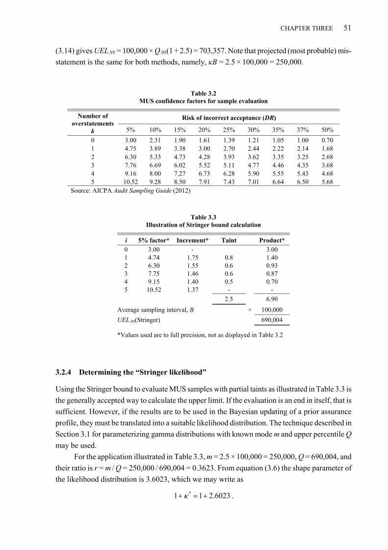
CHAPTER THREE 51
(3.14) gives UEL.95 = 100,000 × Q.95(1 + 2.5) = 703,357. Note that projected (most probable) mis-
statement is the same for both methods, namely, κB = 2.5 × 100,000 = 250,000.
Table 3.2 MUS confidence factors for sample evaluation
Number of overstatements
k
Risk of incorrect acceptance (DR)
5% 10% 15% 20% 25% 30% 35% 37% 50%
0 3.00 2.31 1.90 1.61 1.39 1.21 1.05 1.00 0.70 1 4.75 3.89 3.38 3.00 2.70 2.44 2.22 2.14 1.68 2 6.30 5.33 4.73 4.28 3.93 3.62 3.35 3.25 2.68 3 7.76 6.69 6.02 5.52 5.11 4.77 4.46 4.35 3.68 4 9.16 8.00 7.27 6.73 6.28 5.90 5.55 5.43 4.68 5 10.52 9.28 8.50 7.91 7.43 7.01 6.64 6.50 5.68
Source: AICPA Audit Sampling Guide (2012)
Table 3.3 Illustration of Stringer bound calculation
i 5% factor* Increment* Taint Product*
0 3.00 - 3.00 1 4.74 1.75 0.8 1.40 2 6.30 1.55 0.6 0.93 3 7.75 1.46 0.6 0.87 4 9.15 1.40 0.5 0.70 5 10.52 1.37 - -
2.5 6.90
Average sampling interval, B × 100,000
UEL.95(Stringer) 690,004
*Values used are to full precision, not as displayed in Table 3.2
3.2.4 Determining the “Stringer likelihood”
Using the Stringer bound to evaluate MUS samples with partial taints as illustrated in Table 3.3 is
the generally accepted way to calculate the upper limit. If the evaluation is an end in itself, that is
sufficient. However, if the results are to be used in the Bayesian updating of a prior assurance
profile, they must be translated into a suitable likelihood distribution. The technique described in
Section 3.1 for parameterizing gamma distributions with known mode m and upper percentile Q
may be used.
For the application illustrated in Table 3.3, m = 2.5 × 100,000 = 250,000, Q = 690,004, and
their ratio is r = m / Q = 250,000 / 690,004 = 0.3623. From equation (3.6) the shape parameter of
the likelihood distribution is 3.6023, which we may write as
*1 1 2.6023 .

52 GAMMA DISTRIBUTIONS IN AUDITING
From (3.3), the scale parameter is
**
250,00096,068
2.6023
mB
.
The Stringer likelihood distribution is therefore
* *( ;1 , ) ( ;1 2.6023, 96,068)g x B g x ,
which can be used to update the prior via Bayes rule. If the prior is negligible, then the posterior
distribution equals the Stringer likelihood distribution and its 95th percentile is 690,004, the same
as UEL.95(Stringer) in Table 3.3.
In classical MUS evaluations, the confidence factors applied are those in the appropriate
DR column in Table 3.2. In a Bayesian evaluation, where the purpose is to parameterize the
gamma likelihood distribution, the 5% column should be used (assuming 95% is the desired pos-
terior level of assurance).27
3.3 GUAM as a generalization of ARM
As noted in Section 1.3.2, ARM is a simplistic multiplicative model that does not always yield
the correct probabilities provided by Bayes’ rule. Nevertheless ARM equation (1.2) is widely cit-
ed in the auditing literature and used in audit planning—sometimes directly by auditors in the
field and sometimes indirectly through the use of tables that are developed by the auditor’s firm
with ARM as the basis.28 It is therefore a matter of some practical and theoretical interest to know
under what circumstances ARM “works” in the sense of delivering the same probabilities as
Bayes’ rule.
We will see that ARM works if and only if its probabilities RMM, DR, and AR come from
exponential distributions. Because these are gamma distributions (with = 1), it follows as a cor-
ollary that the GUAM model is a true generalization of ARM and that ARM is a special case of
GUAM. To demonstrate this proposition requires a more precise formulation of audit risk in gen-
eral and ARM in particular.
3.3.1 Formulating audit risk and ARM
There are two basic interpretations of audit risk: the discrete and the continuous, both depicted in
Figure 3.3. The discrete interpretation is that total misstatement is either equal to materiality or
zero and the auditor must “stack” the probabilities on the points 0 and T. For example, AR = 5% 27 While in principle it makes no difference which column is used as each just yields a different percentile of the same likelihood distribution, in practice, (a) approximation (3.6) is more accurate at the 95% level than at lower levels, and (b) where there are partial taints, it makes a small difference which column is used because of the nature of the Stringer bound. For consistency across applications it is best to simply use the 5% column. 28 For example, the Haskins & Sells (Deloitte) table described by McCrae (1974) and mentioned in Section 3.1 is based on ARM.
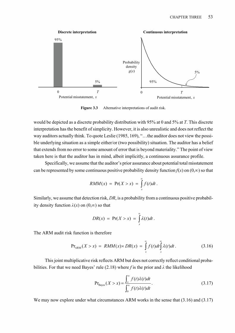
CHAPTER THREE 53
Discrete interpretation Continuous interpretation
Figure 3.3 Alternative interpretations of audit risk.
would be depicted as a discrete probability distribution with 95% at 0 and 5% at T. This discrete
interpretation has the benefit of simplicity. However, it is also unrealistic and does not reflect the
way auditors actually think. To quote Leslie (1985, 169), “…the auditor does not view the possi-
ble underlying situation as a simple either/or (two possibility) situation. The auditor has a belief
that extends from no error to some amount of error that is beyond materiality.” The point of view
taken here is that the auditor has in mind, albeit implicitly, a continuous assurance profile.
Specifically, we assume that the auditor’s prior assurance about potential total misstatement
can be represented by some continuous positive probability density function f (x) on (0,) so that
( ) Pr( ) ( )x
RMM x X x f t dt
.
Similarly, we assume that detection risk, DR, is a probability from a continuous positive probabil-
ity density function λ (x) on (0,) so that
( ) Pr( ) ( )x
DR x X x t dt
.
The ARM audit risk function is therefore
ARMPr ( ) ( ) ( ) ( ) ( )x x
X x RMM x DR x f t dt t dt
. (3.16)
This joint multiplicative risk reflects ARM but does not correctly reflect conditional proba-
bilities. For that we need Bayes’ rule (2.18) where f is the prior and λ the likelihood
Bayes
0
( ) ( )Pr ( )
( ) ( )
xf t t dt
X xf t t dt
. (3.17)
We may now explore under what circumstances ARM works in the sense that (3.16) and (3.17)
95%
5%
0 TPotential misstatement, x
T 0
Probability density
g(x)
Potential misstatement, xT
95%
5%

54 GAMMA DISTRIBUTIONS IN AUDITING
are equal. This is equivalent to determining for what distributions f and λ
0
( ) ( )( ) ( ) for all 0
( ) ( )
x
x x
f t t dtf t dt t dt x
f t t dt
. (3.18)
As an example of where ARM works consider Figure 2.3. Here we have an exponential pri-
or g(x; 1, 100 / 0.7) and an exponential likelihood g(x; 1, 100 / 2.3), which combine via Bayes’ rule
to yield an exponential posterior g(x; 1, 100 / 3.0). To prove the point, we have on the left-hand
side of equation (3.18)
100 100
0.7 2.3
(100) (100) ( ;1,100 / 0.7) ( ;1,100 / 2.3)
.5 .1 .05,
RMM DR g t dt g t dt
e e
and on the right and side, per equation (2.19),
3.0
1000
( ) ( )( ;1,100 / 3.0) .05
( ) ( )
xf t t dt
g t dt ef t t dt
.
Thus ARM and GUAM give the same numerical result.
As an example of where ARM fails, assume that in the previous example the substantive
test is a MUS sample with one error, so k = 1. Per (3.10) the standardized likelihood function is
g(x; 2, 100 / 2.3) and per (2.19) the posterior distribution is g(x; 2, 100 / 3.0). Therefore, the correct,
Bayesian audit risk is
100
( ;2,100 / 3.0) .2g x dx
.
However, ARM yields
100 100
(100) (100) ( ;1,100 / 0.7) ( ;2,100 / 2.3)
.5 .33 .165.
RMM DR g x dx g x dx
Therefore, audit risk that is actually 20% per Bayes’ rule is 16.5% per ARM. Kinney (1983) has
also commented on the understatement of risk when ARM is used. This tendency to understate
audit risk is further illustrated in Section 3.4.
3.3.2 ARM works if and only if its probabilities are from exponential distributions
We now prove the more general proposition that ARM works if and only if its probabilities RMM
and DR are from exponential distributions. More formally, if f and λ are continuous positive
probability distributions on (0,) then equation (3.18) is satisfied (i.e., ARM works) if and only if
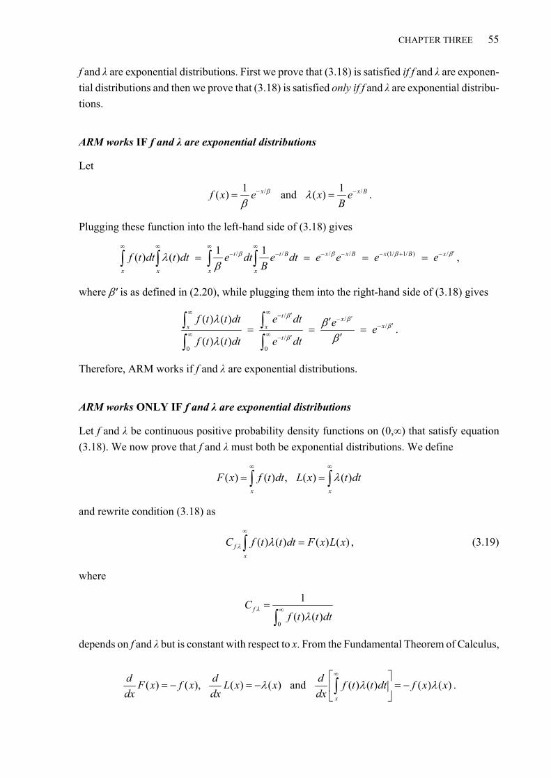
CHAPTER THREE 55
f and λ are exponential distributions. First we prove that (3.18) is satisfied if f and λ are exponen-
tial distributions and then we prove that (3.18) is satisfied only if f and λ are exponential distribu-
tions.
ARM works IF f and λ are exponential distributions
Let
/ /1 1( ) and ( )x x Bf x e x e
B
.
Plugging these function into the left-hand side of (3.18) gives
/ / / / (1/ 1/ ) /1 1( ) ( ) t t B x x B x B x
x x x x
f t dt t dt e dt e dt e e e eB
,
where ʹ is as defined in (2.20), while plugging them into the right-hand side of (3.18) gives
/ /
/
/
0 0
( ) ( )
( ) ( )
t xxx x
t
f t t dt e dt ee
f t t dt e dt
.
Therefore, ARM works if f and λ are exponential distributions.
ARM works ONLY IF f and λ are exponential distributions
Let f and λ be continuous positive probability density functions on (0,∞) that satisfy equation
(3.18). We now prove that f and λ must both be exponential distributions. We define
( ) ( ) , ( ) ( )x x
F x f t dt L x t dt
and rewrite condition (3.18) as
( ) ( ) ( ) ( )f
x
C f t t dt F x L x
, (3.19)
where
0
1
( ) ( )fC
f t t dt
depends on f and λ but is constant with respect to x. From the Fundamental Theorem of Calculus,
( ) ( ), ( ) ( ) and ( ) ( ) ( ) ( )x
d d dF x f x L x x f t t dt f x x
dx dx dx
.
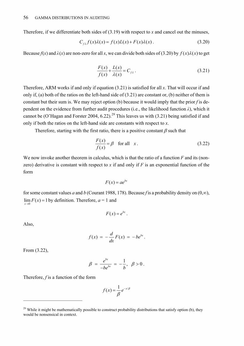
56 GAMMA DISTRIBUTIONS IN AUDITING
Therefore, if we differentiate both sides of (3.19) with respect to x and cancel out the minuses,
( ) ( ) ( ) ( ) ( ) ( )fC f x x f x L x F x x . (3.20)
Because f (x) and λ (x) are non-zero for all x, we can divide both sides of (3.20) by ( ) ( )f x x to get
( ) ( )
( ) ( ) f
F x L xC
f x x . (3.21)
Therefore, ARM works if and only if equation (3.21) is satisfied for all x. That will occur if and
only if, (a) both of the ratios on the left-hand side of (3.21) are constant or, (b) neither of them is
constant but their sum is. We may reject option (b) because it would imply that the prior f is de-
pendent on the evidence from further audit procedures (i.e., the likelihood function λ), which it
cannot be (O’Hagan and Forster 2004, 6.22).29 This leaves us with (3.21) being satisfied if and
only if both the ratios on the left-hand side are constants with respect to x.
Therefore, starting with the first ratio, there is a positive constant such that
( )
for all( )
F xx
f x . (3.22)
We now invoke another theorem in calculus, which is that the ratio of a function F and its (non-
zero) derivative is constant with respect to x if and only if F is an exponential function of the
form
( ) bxF x ae
for some constant values a and b (Courant 1988, 178). Because f is a probability density on (0,∞),
0lim ( ) 1x
F x
by definition. Therefore, a = 1 and
( ) bxF x e .
Also,
( ) ( ) bxdf x F x be
dx .
From (3.22),
1
, 0bx
bx
e
be b
.
Therefore, f is a function of the form
/1( ) xf x e
29 While it might be mathematically possible to construct probability distributions that satisfy option (b), they would be nonsensical in context.

CHAPTER THREE 57
for some > 0, in other words an exponential probability distribution. Similarly, λ is an exponen-
tial probability distribution of the form
/1( ) x Bx e
B
for some B > 0.
3.3.3 Conclusion
We may conclude, therefore, that ARM works if and only if the probabilities RMM and DR are
both from exponential probability distributions. Consequently, when practitioners use ARM to
plan an audit they are implicitly assuming a model that involves exponential distributions, in oth-
er words a special case of the GUAM model. In that strong sense, therefore, the GUAM model is
a generalization of the profession’s generally accepted audit risk model.
3.4 Comparison of GUAM and ARM in audit planning practice
In Section 3.3 we saw an example of how ARM can understate the true audit risk if misstatements
are detected when the audit plan is designed assuming none will be detected. In this section we
see how use of ARM can result in an understatement of true audit risk even if the audit plan con-
templates that misstatements will be detected. The design parameters for MUS tabulated in the
AICPA Audit Sampling Guide (AICPA 2012, 143) are used to illustrate.
The table, reproduced in the top panel of Table 3.4, contains confidence factors, denoted F,
which are used to derive sample sizes, denoted n, based on T / Y (the ratio of materiality to popu-
lation size). The columns represent various values of RMM and DR such that RMM × DR = 5%
(AR). RMM ranges from 100% to 10% and DR from 5% to 50%.30 The rows represent r = m / T,
the ratio of anticipated projected misstatement to T ranging from 0 to 0.60. The workings of the
table are explained in the sampling guide and the computation of the F factors is explained in the
technical notes (Stewart 2012) that accompany the sampling guide. Sample size is determined by
locating the F factor in the cell defined by column value DR and row value r and dividing F by
T / Y to get
/
Fn
T Y . (3.23)
For example, if RMM = 50% (DR = 10%), T / Y = 0.01, and r = 0.4 (i.e., it is anticipated that pro-
jected misstatement will be 40% of T and thus 0.4% of Y), then F = 5.72 and the required sample 30 Only the DR row is included in the original AICPA table, where it is labeled as Risk of Incorrect Acceptance. The DR risks range from 5% to 50% in increments of 5%, except that 37% is used in place of 40%. This is be-cause sampling plans frequently use an associated RP factor of exactly 1.0, which corresponds to approximately DR = 37% as shown in the r = 0 row. The RMM row in Table 3.4 has been computed from DR and an assumed acceptable AR of 5%. A different AR would result in a different lower panel in the table.

58 GAMMA DISTRIBUTIONS IN AUDITING
Table 3.4 True audit risk in audit planning: an example based on the AICPA MUS table
Confidence factors source: AICPA Audit Sampling Guide (AICPA 2012)
size is n = 5.72 / 0.01 = 572.31 If the sample goes according to plan then the overall audit risk
should be 5% according to ARM, on which the table is based. A comparison of the true audit risk
per Bayes’ rule with the nominal 5% illustrates the divergence of ARM and GUAM in a practical
setting.
The bottom panel of Table 3.4 shows for each corresponding cell in the top panel the true
(Bayesian) audit risk associated with the sample design. It can be seen that the true audit risk
equals the nominal 5% when r = 0. This is because both RMM and DR are represented by expo-
nential distributions in the Bayesian model and therefore, as shown in Section 3.3, ARM and
GUAM give the same results. The true audit risk also equals the nominal 5% when RMM =
100%. This is because the GUAM representation of RMM = 100% is a negligible prior in which
all the assurance (and risk) is represented by the sample results. In all other cells it can be seen 31 Note that if r = 0 then equation (3.23) reduces to equation (3.13).
Confidence factors (F ) for MUS design, based on ARM to achieve AR = 5%
RMM 100.0% 50.0% 33.3% 25.0% 20.0% 16.7% 14.3% 13.5% 10.0%
DR 5.0% 10.0% 15.0% 20.0% 25.0% 30.0% 35.0% 37.0% 50.0%
0.00 3.00 2.31 1.90 1.61 1.39 1.21 1.05 1.00 0.70 0.05 3.31 2.52 2.06 1.74 1.49 1.29 1.12 1.06 0.73 0.10 3.68 2.77 2.25 1.89 1.61 1.39 1.20 1.13 0.77 0.15 4.11 3.07 2.47 2.06 1.74 1.49 1.28 1.21 0.82 0.20 4.63 3.41 2.73 2.26 1.90 1.62 1.38 1.30 0.87 0.25 5.24 3.83 3.04 2.49 2.09 1.76 1.50 1.41 0.92 0.30 6.00 4.33 3.41 2.77 2.30 1.93 1.63 1.53 0.99 0.35 6.92 4.95 3.86 3.12 2.57 2.14 1.79 1.67 1.06 0.40 8.09 5.72 4.42 3.54 2.89 2.39 1.99 1.85 1.14 0.45 9.59 6.71 5.13 4.07 3.29 2.70 2.22 2.06 1.25 0.50 11.54 7.99 6.04 4.75 3.80 3.08 2.51 2.32 1.37 0.55 14.18 9.70 7.26 5.64 4.47 3.58 2.89 2.65 1.52 0.60 17.85 12.07 8.93 6.86 5.37 4.25 3.38 3.09 1.70
True audit risk compared with nominal AR = 5% (heat map)0.00 5.0% 5.0% 5.0% 5.0% 5.0% 5.0% 5.0% 5.0% 5.0%0.05 5.0% 5.1% 5.2% 5.2% 5.2% 5.2% 5.2% 5.2% 5.2%0.10 5.0% 5.2% 5.3% 5.4% 5.4% 5.4% 5.4% 5.4% 5.4%0.15 5.0% 5.4% 5.5% 5.6% 5.7% 5.7% 5.7% 5.6% 5.5%0.20 5.0% 5.5% 5.8% 5.9% 5.9% 5.9% 5.9% 5.9% 5.8%0.25 5.0% 5.7% 6.0% 6.2% 6.2% 6.3% 6.2% 6.2% 6.1%0.30 5.0% 5.8% 6.2% 6.5% 6.6% 6.6% 6.6% 6.6% 6.3%0.35 5.0% 6.0% 6.5% 6.8% 7.0% 7.0% 7.0% 7.0% 6.7%0.40 5.0% 6.2% 6.9% 7.2% 7.4% 7.5% 7.5% 7.4% 7.1%
0.45 5.0% 6.4% 7.2% 7.7% 7.9% 8.0% 8.0% 8.0% 7.5%0.50 5.0% 6.6% 7.6% 8.2% 8.5% 8.7% 8.6% 8.6% 8.0%0.55 5.0% 6.9% 8.0% 8.8% 9.2% 9.4% 9.4% 9.3% 8.6%0.60 5.0% 7.1% 8.5% 9.4% 10.0% 10.2% 10.2% 10.2% 9.4%
r =
Exp
ecte
d M
isst
atem
ent /
Tr
= E
xpec
ted
Mis
stat
emen
t / T

CHAPTER THREE 59
that true audit risk exceeds and in some cases is more than double the nominal 5% risk. The table
is shaded as a heat map to highlight differences between true and nominal risk.
A note on the Bayesian calculation of audit risk
The calculation of true risk is performed by determining the prior, likelihood, and posterior distri-
butions for the sample designs implied by each cell in the table and then using the posteriors to
calculate the true risk as Pr(X > T). We start with RMM, which, from (2.17), can be represented
by a prior exponential distribution
Prior ;1,P
Tg x
R
, (3.24)
where, from (2.16), RP = −ln(RMM). As to the likelihood function to be induced by the planned
MUS, we have from (3.7) and (3.23) that it is a gamma distribution with scale parameter
( / )Y Y T Y T
Bn F F
. (3.25)
From (3.11) its shape parameter is 1 + κ, where κB is the mode (most probable misstatement).
Given that r is the expected ratio of projected misstatement to T, we have κB = rT. Therefore,
from (3.25),
rT
rFB
. (3.26)
Therefore, from (3.25), and (3.26), the planned likelihood function is
Likelihood ;1 ,T
g x rFF
. (3.27)
From (2.20), (3.24), and (3.27) the planned posterior distribution is
Posterior ;1 ,P
Tg x rF
R F
.
Finally, keeping in mind from (2.8) that G(x; , ) = G(x / ; , 1), true audit risk is
Pr( ) 1 ;1 , 1 ( ;1 ,1)PP
TX T G T rF G R F rF
R F
.
For example, using the previous illustration where RMM = 50%, r = 0.40, and F = 5.72 we have
RP = −ln(.5) = 0.7 and
Pr( ) 1 (0.7 5.72;1 0.40 5.72,1) 6.2%X T G ,
which is greater than the nominal AR = 5%.32
32 We can check that DR = 10% as planned. From (3.27), DR = 1 − G(T,1 + r F, T / F) = 1 − G( F,1 + r F, 1) = 1 − G( 5.72,1 + 0.40 × 5.72, 1) = 10%.

60 GAMMA DISTRIBUTIONS IN AUDITING
3.5 The exponential as a maximum entropy prior
In physics, thermodynamic entropy is a measure of the amount of disorder and unpredictability in
a system. In probability theory, information entropy is a measure of how uninformative a proba-
bility distribution is about the random variable whose behavior it describes: the less informative
the distribution the higher its entropy. For a discrete probability distribution p on the set
{x1, x2, …, xN} with pi = p(xi), the entropy of p is defined to be
( ) log( )i iH p p p .33
This definition of entropy, introduced by Shannon (Shannon 1948), resembles Boltzmann’s for-
mula for the thermodynamic notion of entropy.34 Physical systems are expected to evolve into
states of increasing disorder (higher entropy) as they approach equilibrium. In probability and in-
formation theory, H(p) is a measure of the information carried by p, with higher entropy corre-
sponding to less information (more uncertainty). Moreover, Shannon proved that H (p) is essen-
tially the only satisfactory measure of information entropy (Shannon 1948; Jaynes 2003). The en-
tropy of a continuous probability distribution with density function f is defined analogously as
( ) ( ) log( ( ))H f f x f x dx
(O’Hagan and Forster 2004, 5.40).
When we have limited knowledge about a prior probability distribution we may apply the
principle of maximum entropy to select a probability density function whose entropy is as large as
possible subject what is known (Jaynes 1957, 1957a, 1963). This principle leads to the selection
of a probability density function that is consistent with our knowledge and introduces no unwar-
ranted information. Any probability density function that satisfies the constraints but has smaller
entropy contains more information (less uncertainty), and thus says something stronger than what
we know or assume (Conrad 2005). The maximum entropy distribution is “maximally noncom-
mittal with regard to missing information” (Jaynes 1957).
Consider the exponential distribution with mean given by equation (2.14). Its entropy is
/ /
0
1 1( (1, )) ln 1 ln( )x xH g e e dx
.
It can be shown that for any continuous probability distribution f on (0,∞) with mean ,
( ) 1 ln( )H f , (3.28)
with equality if and only if f is exponential (O’Hagan and Forster 2004, 5.42; Conrad 2005). In 33 The base of the logarithm is arbitrary. In information theory, where pi is the probability of a binary digit, base 2 is usually the most convenient. In probability theory base e is usually used. Also, it is defined that 0 log(0) = 0. 34 In thermodynamics, pi is the probability that particle i will be in a given microstate and all of the pi are evalu-ated for the same macrostate of the system.

CHAPTER THREE 61
other words, when a mean value is known, assumed or implied, the exponential distribution has
greater entropy than any other continuous distribution on (0,∞). Various continuous distributions
on (0,∞) with the same mean are depicted in Figure 3.4. The maximum entropy distribution is the
exponential thick grey curve. If the mean is = = 1 then from (3.28) the entropy of the expo-
nential distribution is 1 + ln(1) = 1 + 0 = 1 and the entropy is less than 1 for any other continuous
distribution on (0,∞) with mean 1.35
We saw in Sections 2.1.1 and 2.3.4 that specifying a priori that the risk of material mis-
statement is RMM is equivalent to specifying a priori that T is the 100P-th percentile of some
probability distribution where P = 1 − RMM. Absent any additional information, that prior proba-
bility can be represented by an exponential distribution g(x; 1, ), where = T / RP is the scale pa-
rameter and also the mean. Because g(x; 1, ) has greater entropy than any other continuous prob-
ability distribution on (0,∞) with mean , it is the natural “default” representation of what is
known in the sense that it is maximally noncommittal with regard to missing information. As was
proved in Section 3.3, if the auditor is using ARM then g(x; 1, ) is also the only distribution for
which ARM yields correct probabilities.
Figure 3.4 Various continuous distributions on (0,∞) with mean . = 1.
3.6 Why gamma distributions? A summary
This and the previous chapter have explained how and why the GUAM model represents audit
assurance with probability distributions from the gamma family. Here we summarize the reasons.
35 From bottom to top in Figure 3.4 according to where the curve intersects with the vertical from the mean, the distributions are gamma with shape ½, exponential, lognormal, folded normal, and gamma with shape 3. There are infinitely many other continuous distributions with the same mean and they all have lower entropy than the exponential.
0
1.5
0 1 2 3 4
f (x)
Potential misstatement, x
= 1

62 GAMMA DISTRIBUTIONS IN AUDITING
Gammas generalize the standard ARM. The ARM gives correct results if and only if its
probabilities come from exponential distributions. Since these are the most basic gamma distribu-
tions (shape = 1) it means that the GUAM model is a true generalization of ARM. Put differently,
ARM is a special case of GUAM. This means that current auditing theory and practice based on
ARM work identically under GUAM. GUAM generalizes a model that auditors are familiar with
and which has been used for audit planning since the 1970s (Section 3.3).
Intuitive fit for prior assurance. The gamma family provides a rich variety of shapes that
are intuitively appealing as models of judgmental prior audit assurance (Sections 2.3 and 3.1).
Furthermore, RMM as conceptualized in ARM directly translates into an appropriate exponential
distribution (Section 2.3.4).
Good likelihood model. When MUS is used for substantive testing, its results induce a
likelihood function that can be naturally interpreted as a gamma distribution. Results from other
types of audit procedures can usually be modeled, at least approximately, by gamma distributions.
The gamma distribution is a conjugate prior for the Poisson distribution and other gamma distri-
butions, meaning that the posterior distribution following transformation via Bayes’ rule is anoth-
er gamma distribution (Section 2.4.1).
Minimal assumptions. If there is no indication of misstatement the exponential is the max-
imum entropy distribution (Section 3.5). Using any other distribution to model the auditor’s prior
requires additional assumptions. In the absence of additional information, Occam’s razor suggests
that the exponential be used. Exponential distributions as zero-misstatement “base case” priors
naturally transform into other exponential or higher-order gamma posteriors via Bayes’ rule and
thus into approximate gammas as those posteriors are aggregated to the group level.
Good aggregation model. In group audits, and potentially in other applications, it is neces-
sary to aggregate assurance over multiple components. This involves the convolution of the com-
ponent assurance profiles. As explained in Chapter 6, the GUAM model provides a gamma ap-
proximation to the convolution that is good enough for any group likely to be encountered in
practice.
3.7 The beta distribution as an alternative to the gamma
Of course gammas are not the only probability distributions that could possibly be used to repre-
sent audit assurance, though they have appealing attributes as summarized in the previous subsec-
tion. The beta family of distributions provides an alternative. It has been explored by a number of
authors (e.g., Teitlebaum 1973; Steele 1992; Wille 2003) usually in its role as a conjugate prior to
the binomial distribution, which is widely used in audit sampling applications—attributes sam-
pling in particular, but also MUS. This section gives a brief exposition of the beta distribution that
parallels the development of the gamma-based GUAM model.

CHAPTER THREE 63
3.7.1 The beta distribution
For a continuous random variable X such that 0 < X < Y, the beta distribution is defined by the
probability density function
1 1
( ) 1( ; , , ) 1 for 0 and , 0
( ) ( )
p qp q x x
b x p q Y x Y p qp q Y Y Y
(3.29)
(Johnson et al. 1995, 210).36 Both p and q are shape parameters and Y is the scale parameter. In
auditing, the beta distribution usually arises as a conjugate prior for the binomial distribution.
This discrete distribution is used to describe the probability of obtaining k errors in a sample of n
items (AICPA 2012) from a population with error rate x / Y, where x is the amount of error and Y
is the size of the population. That is,
( ; , / ) 1 for 0,1, 2, ,k n kn x x
Binomial k n x Y k nk Y Y
. (3.30)
If X has a beta distribution b (x; p, q, Y), its mode is
1
Mode( ) , , 12
pX Y p q
p q
, (3.31)
its expected value is
( )p
E X Yp q
, (3.32)
and its variance is
22
Var( )( ) ( 1)
pqX Y
p q p q
(3.33)
(Johnson et al. 1995, 222).
As with the gamma distribution, the parameters of the beta distribution can be expressed in
terms of the expected value and variance. From (3.32) we have
( )E X p
Y p q
,
and from (3.33),
2
Var( ) 1 11
1 1
X p q p p
Y p q p q p q p q p q p q
.
36 Some authors (including Johnson et al.) define the range of x as 0 x Y. Because the function is undefined for x = 0 if p < 1 and for x = 1 if q < 1, I use the open interval, which is consistent with my treatment of the gamma. It makes no practical difference, especially in auditing applications, where, invariably, p ≥ 1 and q ≥ 1.

64 GAMMA DISTRIBUTIONS IN AUDITING
Therefore,
2
( ) ( )1
1Var( )
E X E XY Y
p qX
Y
, (3.34)
2
2
( ) ( )1
( )Var( )
E X E XE XY Y
pX Y
Y
, (3.35)
and
( )q p q p .
In general, there is no closed form expression for the cumulative beta probability distribu-
tion or the percentile function. However, values can be obtained using the Excel BetaDist and
BetaInv functions, respectively. For the CDF,
0
( ; , , ) ( ; , , ) BetaDist( / , , )x
B x p q Y B t p q Y dt x Y p q . (3.36)
For the percentile function,
( , , ) BetaInv( , , )Px Q p q Y Y P p q . (3.37)
The beta distribution (3.29) with Y = 1 is known as the standard beta distribution and the
random variable X, which varies between 0 and 1, can be interpreted as the error rate. It is in this
form that the beta distribution usually appears in Bayesian treatments of attributes sampling
(Steele 1992). The parameter Y = 1 is usually omitted. Several b (x; p, q) distributions are depicted
in Figure 3.5.
The beta family of distributions includes an incredibly rich variety of density functions. Be-
sides everyday distributions such as those in Figure 3.5, they include left-skew distributions (i.e.,
distributions that peak to the right of the half-way mark), U-shaped distributions with modes at
both ends, and symmetrical bell-shaped and umbrella-shaped distributions. Specimens from the
beta distribution zoo are depicted in Figure 3.6. Johnson et al. (1995, 220-221) show these and
more shapes. Many are unlikely to be useful in audit applications, which are ordinarily limited to
right-skew distributions with most of the probability distributed over the low end of the range,
such as those depicted in Figure 3.5.
The beta distribution b (x; 1, 1), depicted in Figure 3.5 and Figure 3.6 as a flat line at height 1
(i.e., 1 / Y) above the x axis, is the uniform distribution on the interval (0, 1). In audit assurance
terms it represents a non-informative prior, where in the auditor’s judgment every value of X is
equally likely. It plays a similar role to the negligible exponential prior discussed in Section 2.4.2.

CHAPTER THREE 65
It is also the maximum entropy distribution on (0, 1), just as the exponential distribution g(x; 1, )
has maximum entropy among continuous distributions on (0, ∞) with mean (Conrad 2005).
Figure 3.5 Various beta distributions b (x; p, q).
Figure 3.6 Further specimens from the beta distribution zoo.
3.7.2 Bayesian analysis
Suppose a prior b (x; p, q, Y) has been established.37 If a sample of n items containing k errors is
selected from the population of size Y, then a likelihood function is induced that is essentially the
binomial distribution interpreted as a function of x for fixed k rather than as the probability of k
37 The parameters can be calculated in a manner similar to that explained in Section 3.1 making use of the mode (3.31), and the percentile function (3.37) as implemented in Excel or an approximation formula.
0
10
0 .1 .2 .3 .4 .5
b(x)
Potential error rate, x
p = 1, q = 10
p = 2, q = 20
p = 1, q = 1
p = 6, q = 30
0
1
2
3
4
0 .1 .2 .3 .4 .5 .6 .7 .8 .9 1.0
b(x)
Potential error rate, x

66 GAMMA DISTRIBUTIONS IN AUDITING
errors for fixed x. From (3.30), the likelihood function is
( | ; , ) 1 , 0k n kn x x
x k n Y x Yk Y Y
.
Following an argument similar to that in Section 3.2.1, and recalling from (2.2) that k! = Γ(k + 1)
and (n − k)! = Γ(n − k + 1),
(1 ) 1
(1 ) 1
! 1 ( 1)!1 1 1
!( )! 1 !( )!
(1 ) ( 1) 11
1 (1 ) ( 1)
1
k n k k n k k n k
k n k
n x x n x x n x x
k Y Y k n k Y Y n k n k Y Y
k n kY x x
n k n k Y Y Y
Y
n
( ;1 , 1, ).b x k n k Y
Because it is a probability distribution that is a scalar multiple of the likelihood function, we may
describe b (x;1 + k, n − k + 1, Y) as the likelihood distribution induced by the sample. Plugging this
likelihood and the prior b (x; p, q, Y) into Bayes’ rule and following an argument similar to that in
Section 2.4.1, we find that the posterior is
0
( ; , , ) ( ;1 , 1, )( ; , , ) ( ; , , )
( ; , , ) ( ;1 , 1, )Y
b x p q Y b x k n k Yb x p q Y b x p k n k q Y
b t p q Y b t k n k Y dt
.
Note that if the prior is the non-informative, uniform b (x; 1, 1, Y) then the posterior is the
same as the likelihood distribution, namely
( ;1 , 1, )b x k n k Y . (3.38)
Figure 3.7 Beta likelihood and posterior induced by an attribute sample and a uniform prior.
0
25
0 .01 .02 .03 .04 .05 .06 .07 .08 .09 .10 .11 .12
b(x)
Potential error rate, x
Uniform Priorb(x;1,1)
Likelihood = Posteriorb(x;4,98)
95th Percentile .075Mode .03
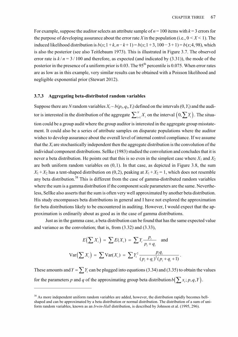
CHAPTER THREE 67
For example, suppose the auditor selects an attribute sample of n = 100 items with k = 3 errors for
the purpose of developing assurance about the error rate X in the population (i.e., 0 < X < 1). The
induced likelihood distribution is b (x; 1 + k, n − k + 1) = b (x; 1 + 3, 100 − 3 + 1) = b (x; 4, 98), which
is also the posterior (see also Teitlebaum 1973). This is illustrated in Figure 3.7. The observed
error rate is k / n = 3 / 100 and therefore, as expected (and indicated by (3.31)), the mode of the
posterior in the presence of a uniform prior is 0.03. The 95th percentile is 0.075. When error rates
are as low as in this example, very similar results can be obtained with a Poisson likelihood and
negligible exponential prior (Stewart 2012).
3.7.3 Aggregating beta-distributed random variables
Suppose there are N random variables Xi ~ b (pi, qi, Yi) defined on the intervals (0, Yi) and the audi-
tor is interested in the distribution of the aggregate 1
N
iiX
on the interval 0, iY . The situa-
tion could be a group audit where the group auditor is interested in the aggregate group misstate-
ment. It could also be a series of attribute samples on disparate populations where the auditor
wishes to develop assurance about the overall level of internal control compliance. If we assume
that the Xi are stochastically independent then the aggregate distribution is the convolution of the
individual component distributions. Sellke (1983) studied the convolution and concludes that it is
never a beta distribution. He points out that this is so even in the simplest case where X1 and X2
are both uniform random variables on (0, 1). In that case, as depicted in Figure 3.8, the sum
X1 + X2 has a tent-shaped distribution on (0, 2), peaking at X1 + X2 = 1, which does not resemble
any beta distribution.38 This is different from the case of gamma-distributed random variables
where the sum is a gamma distribution if the component scale parameters are the same. Neverthe-
less, Sellke also asserts that the sum is often very well approximated by another beta distribution.
His study encompasses beta distributions in general and I have not explored the approximation
for beta distributions likely to be encountered in auditing. However, I would expect that the ap-
proximation is ordinarily about as good as in the case of gamma distributions.
Just as in the gamma case, a beta distribution can be found that has the same expected value
and variance as the convolution; that is, from (3.32) and (3.33),
( ) ii i i
i i
pE X E X Y
p q
and
22
Var Var( )( ) ( 1)
i ii i i
i i i i
p qX X Y
p q p q
.
These amounts and iY Y can be plugged into equations (3.34) and (3.35) to obtain the values
for the parameters p and q of the approximating group beta distribution ; , ,ib x p q Y .
38 As more independent uniform random variables are added, however, the distribution rapidly becomes bell-shaped and can be approximated by a beta distribution or normal distribution. The distribution of a sum of uni-form random variables, known as an Irwin-Hall distribution, is described by Johnson et al. (1995, 296).
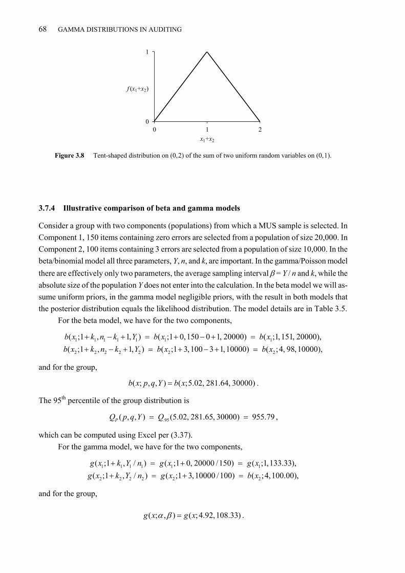
68 GAMMA DISTRIBUTIONS IN AUDITING
Figure 3.8 Tent-shaped distribution on (0, 2) of the sum of two uniform random variables on (0, 1).
3.7.4 Illustrative comparison of beta and gamma models
Consider a group with two components (populations) from which a MUS sample is selected. In
Component 1, 150 items containing zero errors are selected from a population of size 20,000. In
Component 2, 100 items containing 3 errors are selected from a population of size 10,000. In the
beta/binomial model all three parameters, Y, n, and k, are important. In the gamma/Poisson model
there are effectively only two parameters, the average sampling interval = Y / n and k, while the
absolute size of the population Y does not enter into the calculation. In the beta model we will as-
sume uniform priors, in the gamma model negligible priors, with the result in both models that
the posterior distribution equals the likelihood distribution. The model details are in Table 3.5.
For the beta model, we have for the two components,
1 1 1 1 1 1 1
2 2 2 2 2 2 2
( ;1 , 1, ) ( ;1 0,150 0 1, 20000) ( ;1,151, 20000),
( ;1 , 1, ) ( ;1 3,100 3 1,10000) ( ;4, 98,10000),
b x k n k Y b x b x
b x k n k Y b x b x
and for the group,
( ; , , ) ( ;5.02, 281.64, 30000)b x p q Y b x .
The 95th percentile of the group distribution is
.95( , , ) (5.02, 281.65, 30000) 955.79PQ p q Y Q ,
which can be computed using Excel per (3.37).
For the gamma model, we have for the two components,
1 1 1 1 1 1
2 2 2 2 2 2
( ;1 , / ) ( ;1 0, 20000 /150) ( ;1,133.33),
( ;1 , / ) ( ;1 3,10000 /100) ( ;4,100.00),
g x k Y n g x g x
g x k Y n g x b x
and for the group,
( ; , ) ( ;4.92,108.33)g x g x .
0
1
0 1 2
f (x1+x2)
x1+x2

CHAPTER THREE 69
The 95th percentile of the group distribution is
.95 .95( ) 108.33 (4.92) 980.14Q Q ,
which can be computed using Excel per (2.10).
The gamma distribution is slightly more conservative than the beta distribution—in this
case increasing the 95th percentile from 955.79 to 980.14, or by about 2.5%. Conversely, if T =
900 (for example) then, under the beta model, assurance that aggregate misstatement does not ex-
ceed T is, per (3.36),
( , , , ) ( / , , ,1) (900 / 30000, 5.02, 281.65) 93.04%B T p q Y B T Y p q B ,
while under the gamma model it is, per (2.8),
( , , ) (900, 4.92,108.33) 92.15%G T G ,
or about a percentage point less than under the beta model.
Table 3.5 Beta and gamma models compared
Factor Ref. Component 1 Component 2 Group
Y 20,000 10,000 30,000
n 150 100
k 0 3
Beta model
p = 1 + k (3.38) 1 4
q = n − k + 1 (3.38) 151 98
Mode(X) (3.31) 0 300.00 423.87
E(X) (3.32) 131.58 392.16 523.74
Var(X) (3.33) 17,086.71 36,580.40 53,667.11
Group p + q (3.34) 286.66
Group p (3.35) 5.02
Group q = (p + q) − p 281.64
Group 95th Percentile (3.37) 955.79
Gamma model
= 1 + k (2.20) 1 4
= Y / n (3.7) 133.33 100.00
Mode(X) (2.3) 0 300.00 425.00
E(X) (2.4) 133.33 400.00 533.33
Var(X) (2.5) 17,777.78 40,000.00 57,777.78
Group (2.25) 4.92
Group (2.26) 108.33
Group 95th Percentile (2.10) 980.14

70 GAMMA DISTRIBUTIONS IN AUDITING
The various component and group beta and gamma distributions are depicted in Figure 3.9.
The betas are depicted with solid lines and the gammas with dotted lines. They are obviously
close—with the gammas slightly flatter and more extended than the betas, which is to be expected
because the range of X is infinite for the gammas but 20,000, 10,000, and 30,000, respectively for
the three betas. For larger samples relative to the populations, the differences between betas and
gammas would be more marked.
Figure 3.9 Beta (solid line) and gamma (dotted line) density functions compared.
3.7.5 Potential further developments
In the chapters that follow, the GUAM gamma-based model is used to derive a method for deter-
mining component materiality. While I have not attempted a parallel development using beta dis-
tributions, I have no reason to doubt that it can be done. However, I believe that the resulting
method will be more complex for the end user as there are more parameters involved. Also, I
doubt that it would produce significantly better results in most cases, as the beta and gamma dis-
tributions are quite close provided that contemplated misstatement and component materiality are
small relative to component size—as they ordinarily will be. Nevertheless, there may be circum-
stances in which a beta-based method is preferable and I think it is worth researching.
0
.003
0 500 1000 1500
b(x)g(x)
Potential misstatement, x1, x2, x = x1+x2
Component 1: b(x1; 1, 151, 20000)g(x1; 1, 133.33)
Component 2: b(x2; 4, 98, 10000)g(x2; 4, 100)
Group: b(x; 5.02, 281.64, 30000),g(x; 4.92, 108.33)

71
CHAPTER 4 The GUAM Method for Determining Com-ponent Materiality
The GUAM method for determining component materiality applies the Bayesian model described
in Chapter 2. The method works backwards from the target group posterior assurance profile to
determine optimal component posteriors, and from those determines an appropriate set of compo-
nent materiality amounts. This chapter describes the GUAM method in the case of groups with
relatively simple structures and controls. Further practical issues, complexities, and opportunities
for optimization are discussed in Chapter 7.
4.1 Model assumptions
This section explains the assumptions made in the development of the GUAM method for deter-
mining component materiality.
Component audits. It is assumed that each of the N components in the group will be audit-
ed using component materiality. As indicated in Section 1.5.2, ISA 600 requires audits only for
components that are individually financially significant and permits various alternatives for other
components. However, audits are the assurance “gold standard” and are always permitted if not
required. Also, as previously indicated, the number of components for which component materi-
ality is required to be determined is typically fairly small, and although the GUAM method scales
to arbitrarily large groups we will assume relatively small groups for illustrative purposes.
Consistent measure of component size. It is assumed that there is a consistent measure of
relative component size across the group, denoted Yi (e.g., total revenues or total assets). Size is
used by the GUAM algorithm to determine component materiality amounts that minimize the to-
tal variable cost of the group audit. What matters therefore is that, all other things being equal, the
variable cost of auditing the component should ideally be directly proportional to size. For exam-
ple, for a given component materiality amount the variable cost of performing the component au-
dit should double if the component size doubles and halve if the component size halves.
Component misstatement and materiality. It is assumed that total undetected misstate-
ment in each Component i is a positive-valued random variable Xi and that group total undetected

72 THE GUAM METHOD FOR DETERMINING COMPONENT MATERIALITY
misstatement is the random variable iX .39 The group auditor determines component materiali-
ty, denoted Ti for Component i, and we refer to the N-tuple (T1, T2, …, TN) as a component materi-
ality combination. In planning the audit, the group auditor aims to achieve the overall audit objec-
tive expressed as Pr iX T = .95 for the group. Similarly, the component auditor’s objective
for Component i is expressed as PR(Xi Ti) = .95. Note that instead of keeping assurance constant
at 95% and determining component materiality, the group auditor could achieve the same objec-
tive by setting component materiality at some amount and determining the appropriate assurance
level (Kinney 1989).
Misstatements corrected. It is assumed that all detected misstatements are corrected by the
client to the satisfaction of the component and group auditors and that such corrections are to the
misstatements actually found and do not include blanket adjustments to cover best estimates of
total misstatement. This means that Xi represents the potential magnitude of undetected compo-
nent misstatement, something that can only be known probabilistically.
Stochastic independence. The subjective notion of probability induces a very simple con-
cept of independence: two random variables are independent if learning the value of one does not
change one’s belief about the other (O’Hagan and Forster 2004, 4.5). It is assumed that the Xi are
stochastically independent random variables. For separately managed components and absent any
ex ante belief that systemic management fraud or other misstatement is present, independence is a
reasonable planning assumption. Indeed, all other relevant prior audit research of which I am
aware makes a similar assumption about stochastic independence, though the assumption is not
always explicitly stated (Zuber et al. 1983; Boritz et al. 1993; Dutta and Graham 1998; Glover et
al. 2008a and 2008b).
Group auditor’s prior component assurance. It is assumed that the group auditor evalu-
ates prior component risk/assurance based on group-level controls and inherent factors, as de-
scribed in Section 1.6, and that the assurance can be expressed as an exponential distribution
g(xi; 1, i). If the group auditor cannot rely or chooses not to rely on group-level controls because
the component is high risk or for other reasons, the group auditor’s prior component assurance is
treated as “negligible prior assurance” as defined in Section 2.4.2.
4.2 Determining component materiality
As indicated in Chapter 1, ISA 600 states that the purpose of establishing component materiality
is to “reduce to an appropriately low level the probability that the aggregate of uncorrected and
undetected misstatements in the group financial statements exceeds materiality for the group fi-
nancial statements as a whole.” We define achieved group assurance (AGA) to be the comple-
39 In practice, certain audit procedures are performed directly on the consolidated financial statements using group materiality, and it is therefore a simplification to equate the sum of component total misstatement with total group misstatement.

CHAPTER FOUR 73
ment of that probability and assume that the group auditor’s assurance objective is to achieve
AGA = 95%. To achieve this objective, the group auditor must achieve component posterior as-
surance profiles ( ;1, )i ig x that aggregate to a posterior group assurance profile ( ; , )ig x that
has a 95th percentile equal to group materiality T. That is,
.95 ( )Q T . (4.1)
The group parameters ʹ and ʹ are derived from the parameters of the component distributions
via equations (2.25) and (2.26). The key to the GUAM method is determining target component
posteriors ( ;1, )i ig x that aggregate to a group posterior ( ; , )ig x that satisfies equation (4.1).
4.2.1 Constructing target component posteriors
We start with the simplest case and then generalize it. If the group consists of N identical compo-
nents, their target posterior distributions are of the form ( ;1, )ig x . From (2.29) the group poste-
rior assurance profile is ( ; , )ig x N , and its 95th percentile is ʹ Q.95(N). To satisfy equation
(4.1) this percentile must equal T and we must therefore achieve
.95 ( )i
T
Q N (4.2)
as the scale parameter of each component assurance profile. In other words, if the group auditor
achieves a posterior assurance profile ( ;1, )i ig x for each Component i, where i is determined
by (4.2), then, when those posteriors are aggregated, the achieved group posterior assurance pro-
file is ( ; , )ig x N . By construction, therefore, ʹQ.95(N) = T and group assurance objective
(4.1) is achieved. For example, for a two-component group, N = 2, Q.95(2) = 4.74, ʹ = T / 4.74,
and the target assurance profile for each component is g(xi; 1, T / 4.74). By construction, these two
posteriors aggregate to g(x1 + x2; 2, T / 4.74) for the group, and the group 95th percentile is
.95 .95( ) (2) 4.744.74 4.74
T TQ Q T
as required. Assuming the audit goes as planned, AGA = 95% and the group assurance objective
will be accomplished. This is the example depicted in Figure 2.5 with T = 100.
We now generalize to nonidentical components. A clue about how this is done comes from
rewriting equation (4.2) as
.95
11/
i
T
QN
, (4.3)
and interpreting the factor 1 / N as a relative weight that is assigned to each of the N identical
components. The weights obviously sum to 1. We generalize (4.3) to nonidentical components by

74 THE GUAM METHOD FOR DETERMINING COMPONENT MATERIALITY
replacing 1 / N with positive weights wi that sum to 1. In the general case, therefore, we construct
target component posteriors ( ;1, )i ig x , where
.95
for 1,2, ,(1/ )i
i
Ti N
Q w . (4.4)
The group posterior, the distribution of iX , is the convolution of these component posteriors
and is approximated by ( ; , )ig x where ʹ and ʹ are defined by equations (2.25) and (2.26).
In the case of equal weights, wi = 1 / N and equation (4.1) is satisfied exactly. In the case of
unequal weights, equation (4.1) is satisfied approximately rather than exactly, so that (4.1) should
be rewritten as
.95 ( )Q T (4.5)
and AGA 95%. As we will see in Chapter 6, the approximation is very good for any group like-
ly to be encountered in practice—regardless of how the components are weighted. In considering
the appropriateness of approximations, it is healthy to keep in mind that the subject is auditing,
where professional judgment is paramount but usually imprecise.
4.2.2 Weighting components
While any combination of positive weights summing to one will result in a set of component pos-
teriors that achieves the group assurance objective (AGA 95%), they are not all equally efficient
and some will result in much more work (and cost) than is necessary to meet the group assurance
objective. An important feature of the GUAM method is the ability to choose weights that also
achieve secondary objectives—usually minimizing group audit costs. Section 6.3 shows that, ab-
sent any other constraints, group audit costs are minimized if components are weighted approxi-
mately in proportion to the square root of size, that is,
ii
j
Yw
Y
, (4.6)
where Yi is Revenues or some other appropriate financial benchmark. This result is derived as the
solution to a classic constrained optimization problem. Chapter 7 will show how weights can be
adjusted to deal with practical issues such as components that require a specific materiality
amount due to statutory audit requirements, or significant differences in the costs of auditing dif-
ferent components.40 If the components are identical and there are no other constraints then (4.6)
simplifies to wi = 1 / N.
40 If the variable cost per unit audited varies from component to component, then Yi can be replaced by Yi times the variable cost per unit for Component i (shown in Section 5.2).

CHAPTER FOUR 75
4.2.3 Relationship between group and component auditor perspectives
How much assurance the group auditor needs from the auditor of Component i depends on
The component assurance the group auditor has to start with, represented by the prior as-
surance profile for the component, g(xi; 1, i) and
The component assurance the group auditor ultimately requires from all sources, represent-
ed by the target posterior assurance profile for the component, ( ;1, )i ig x , where i i .
The component auditor must do enough work to transform g(xi; 1, i) into ( ;1, )i ig x . From Bayes’
rule and equation (2.22), this means that the evidence from the component audit must induce a
likelihood distribution g(xi; 1, Bi) with
1
, where1/ 1/i i i
i i
B
. (4.7)
We assume here that i i , otherwise the prior assurance would exceed the target posterior as-
surance and no further work would be necessary. If the likelihood distribution g(xi; 1, Bi) is
achieved for Component i, then the component prior g(xi; 1, i) is updated to the target component
posterior ( ;1, )i ig x as required. If this is achieved for each Component i, for i = 1, 2, …, N, then
the group assurance objective expressed in equation (4.5) is achieved by construction.
The group auditor’s Bayesian perspective is that the component auditor must deliver the
target likelihood distribution, g(xi; 1, Bi). The component auditor’s Bayesian perspective is that
g(xi; 1, Bi) is the target posterior assurance profile for the component audit. To achieve this poste-
rior, the component auditor will evaluate risks and controls to develop a prior and will perform
further audit procedures to achieve the target posterior (the group auditor’s target likelihood).
These different perspectives are illustrated in Figure 4.1. It is important that the group auditor’s
component prior and the component auditor’s component prior do not overlap: the group auditor
and component auditor cannot take credit for the same controls. “Double-dipping” is not allowed.
This is discussed in more detail in Section 4.3.1.
Figure 4.1 Group auditor and component auditor perspectives on the component audit.
Prior Likelihood Posterior
Prior Likelihood Posterior
×
× =
=Group auditor’s view of component
Component auditor’s view of component

76 THE GUAM METHOD FOR DETERMINING COMPONENT MATERIALITY
4.2.4 Computing component materiality
In Bayesian terms the group auditor instructs the auditor of Component i to do enough audit work
to achieve the assurance profile g(xi; 1, Bi)—the group auditor’s required likelihood distribution.
In the language of auditing standards, the group auditor instructs the component auditor to use
component materiality Ti in performing the component audit and to achieve reasonable assurance
that total component misstatement does not exceed Ti. Assuming that both the group and compo-
nent auditor understand that reasonable assurance means 95%, the group auditor can express the
Bayesian requirement as a Ti value by equating Ti to the 95th percentile of g(xi; 1, Bi), namely,
.95 .95(1)i i iT B Q B R . (4.8)
Computationally, the formula for Ti follows from (4.4), (4.7), and (4.8),
.95.95
.95
, where (1/ )(1/ ) /i i
i i i
TR TT Q w
Q w T
. (4.9)
If the group auditor’s component prior is negligible then, by definition, 1 / i 0 and (4.9)
simplifies to
.95
.95 (1/ )ii
TRT
Q w . (4.10)
If, additionally, the N components are equally weighted then wi = 1 / N and (4.10) reduces to
.95
.95 ( )i
TRT
Q N . (4.11)
In this simplest form, Ti is T times the ratio of the target component 95th percentile to the target
group 95th percentile. Broadly speaking, component materiality depends on group materiality and
the relationship between the target component posterior and the target group posterior. For exam-
ple, in the case of the two identical components illustrated in Figure 2.5, N = 2, Q.95(2) = 4.74,
and
3.0
0.63 , 1,24.74iT T T i . (4.12)
As an example of unequal components, consider the case of three components of size
(Y1, Y2, Y3) = (9000, 4000, 1000) where prior assurance is negligible. The optimal component mate-
riality combination using square-root weighting formula (4.6) and component materiality formula
(4.10) is (T1, T2, T3) = (63.15, 47.58, 28.50). The calculation is shown in Table 4.1. If prior assur-
ance is not negligible then equation (4.9) applies instead of (4.10). But before looking at an ex-
ample it will be helpful to explore further the effect of prior assurance on component materiality.

CHAPTER FOUR 77
Table 4.1 Illustrative calculation of Ti
Yi √Yi wi Q.95(1 / wi) Ti
Component 1 9,000 94.87 0.5000 4.7439 63.15 Component 2 4,000 63.25 0.3333 6.2958 47.58 Component 3 1,000 31.62 0.1667 10.5130 28.50
14,000 189.74 1.0000 21.5527 139.23
4.3 The effect of prior assurance on component materiality
This section shows that adjusting component materiality for prior assurance amounts to inflating
it by a factor that depends only on that assurance.
In equation (4.8) we defined component materiality as Ti = BiR.95. Let iT denote component
materiality assuming a negligible prior (i.e., 1 / i 0). Then, from (4.7) and (4.8)
.95i iT R . (4.13)
Dividing (4.8) by (4.13) we get
ˆi i
ii
T B
T
.
Moving iT to the right-hand side of the equation and applying (2.20) per Bayes’ rule, we get
1 1ˆ ˆ ˆ 1i i
i i i i ii i i i
B BT T T B T
B
. (4.14)
We saw in Section 2.4.1 that we can write
i
ii
P
T
R , (4.15)
where Pi = 1 − RMMi. In this context “material” in RMMi means component materiality Ti (ISA
600, paragraph A46).41 From (4.8),
.95
ii
TB
R . (4.16)
41 For RMMi < 100%, the level of prior assurance is Pi = 1 − RMMi, which from (2.16) can be expressed as the R factor
iPR = −ln(1 − Pi).
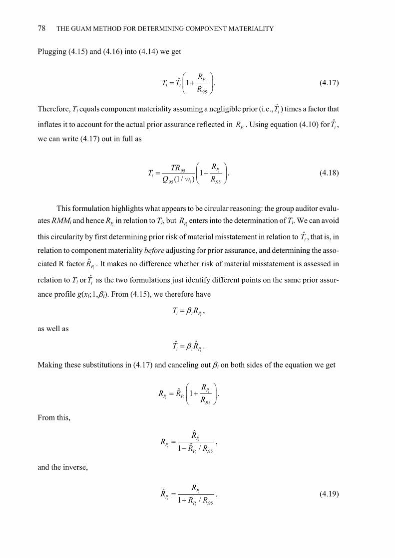
78 THE GUAM METHOD FOR DETERMINING COMPONENT MATERIALITY
Plugging (4.15) and (4.16) into (4.14) we get
.95
ˆ 1 iPi i
RT T
R
. (4.17)
Therefore, Ti equals component materiality assuming a negligible prior (i.e., iT ) times a factor that
inflates it to account for the actual prior assurance reflected in iPR . Using equation (4.10) for iT ,
we can write (4.17) out in full as
.95
.95 .95
1(1/ )
iPi
i
RTRT
Q w R
. (4.18)
This formulation highlights what appears to be circular reasoning: the group auditor evalu-
ates RMMi and henceiPR in relation to Ti, but
iPR enters into the determination of Ti. We can avoid
this circularity by first determining prior risk of material misstatement in relation to iT , that is, in
relation to component materiality before adjusting for prior assurance, and determining the asso-
ciated R factor ˆiPR . It makes no difference whether risk of material misstatement is assessed in
relation to Ti or iT as the two formulations just identify different points on the same prior assur-
ance profile g(xi; 1, i). From (4.15), we therefore have
ii i PT R ,
as well as
ˆ ˆii i PT R .
Making these substitutions in (4.17) and canceling out i on both sides of the equation we get
.95
ˆ 1 i
i i
PP P
RR R
R
.
From this,
.95
ˆ
ˆ1 /i
i
i
PP
P
RR
R R
,
and the inverse,
.95
ˆ1 /
i
i
i
PP
P
RR
R R
. (4.19)
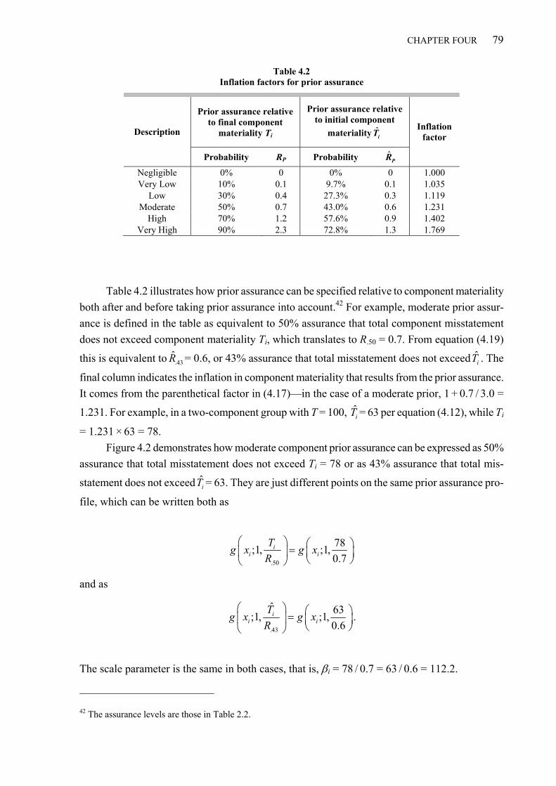
CHAPTER FOUR 79
Table 4.2 Inflation factors for prior assurance
Description
Prior assurance relative to final component
materiality Ti
Prior assurance relative to initial component
materiality iT Inflation
factor
Probability RP Probability ˆPR
Negligible 0% 0 0% 0 1.000 Very Low 10% 0.1 9.7% 0.1 1.035
Low 30% 0.4 27.3% 0.3 1.119 Moderate 50% 0.7 43.0% 0.6 1.231
High 70% 1.2 57.6% 0.9 1.402 Very High 90% 2.3 72.8% 1.3 1.769
Table 4.2 illustrates how prior assurance can be specified relative to component materiality
both after and before taking prior assurance into account.42 For example, moderate prior assur-
ance is defined in the table as equivalent to 50% assurance that total component misstatement
does not exceed component materiality Ti, which translates to R.50 = 0.7. From equation (4.19)
this is equivalent to .43R = 0.6, or 43% assurance that total misstatement does not exceed iT . The
final column indicates the inflation in component materiality that results from the prior assurance.
It comes from the parenthetical factor in (4.17)—in the case of a moderate prior, 1 + 0.7 / 3.0 =
1.231. For example, in a two-component group with T = 100, iT = 63 per equation (4.12), while Ti
= 1.231 × 63 = 78.
Figure 4.2 demonstrates how moderate component prior assurance can be expressed as 50%
assurance that total misstatement does not exceed Ti = 78 or as 43% assurance that total mis-
statement does not exceed iT = 63. They are just different points on the same prior assurance pro-
file, which can be written both as
.50
78;1, ;1,
0.7i
i i
Tg x g x
R
and as
.43
ˆ 63;1, ;1,
0.6i
i i
Tg x g x
R
.
The scale parameter is the same in both cases, that is, i = 78 / 0.7 = 63 / 0.6 = 112.2.
42 The assurance levels are those in Table 2.2.

80 THE GUAM METHOD FOR DETERMINING COMPONENT MATERIALITY
Figure 4.2 Moderate prior assurance in relation to iT and Ti, g(xi; 1, 78 / 0.7).
Figure 4.3 illustrates the determination of Ti for a group with two identical components
where the group auditor has negligible prior assurance for both components. In this case (T1, T2) =
(63, 63). Figure 4.4 illustrates the effect of introducing moderate prior assurance for Component
1. In this case (T1, T2) = (78, 63). In both Figure 4.3 and Figure 4.4, the component posterior as-
surance profiles are g(xi; 1, 63 / 3.0), while the group posterior is g(x1 + x2; ʹ, ʹ) =
g(x1 + x2; 2, 63 / 3.0) with 95th percentile
.95
63( ) 4.74 100
3.0Q
,
which equals T as required. Therefore, a group auditor with a moderate component prior can ap-
ply equation (4.18) to inflate Ti and reduce the required component auditor effort and cost while
achieving the same end result.
Component 1 Component 2 Group
Prior Negligible Negligible
L’hood g(x1; 1, 63 / 3.0) g(x2; 1, 63 / 3.0)
Post g(x1; 1, 100 / 4.74) =
g(x1; 1, 63 / 3.0) g(x2; 1, 100 / 4.74) =
g(x2; 1, 63 / 3.0) g(x1 + x2; 2, 100 / 4.74) =
g(x1 + x2; 2, 63 / 3.0)
Figure 4.3 Determining component materiality with negligible prior assurance.
0
.009
0 100 200 300 400 500
g(xi)
Potential misstatement, xi
50%
43%
ˆ 63i ix T
78i ix T
0
.05
0 50 100 150
g(x1)
x1
T1 = Q.95 = 63
0
.05
0 50 100 150
g(x2)
x2
T2 = Q.95 = 63
0
.05
0 50 100 150
g(x)
x = x1 + x2
T = Q.95 = 100

CHAPTER FOUR 81
Component 1 Component 2 Group
Prior g(x1; 1, 78 / 0.7) Negligible
L’hood g(x1; 1, 78 / 3.0) g(x2; 1, 63 / 3.0)
Post g(x1; 1, 78 / 3.7) = g(x1; 1, 63 / 3.0)
g(x2; 1, 100 / 4.74) = g(x2; 1, 63 / 3.0)
g(x1 + x2; 2, 100 / 4.74) = g(x1 + x2; 2, 63 / 3.0)
Figure 4.4 Determining component materiality with prior assurance for Component 1.
As a further illustration of prior assurance we extend the three-component example in Table
4.1. Instead of assuming negligible priors for all three components, we assume a high level of
prior assurance for Component 1 and a moderate level of prior assurance for Component 2. The
results are depicted in Table 4.3 where the original Ti values from Table 4.1, now designated iT ,
are multiplied by the applicable factors from Table 4.2. The effect is a significant increase in
component materiality for Components 1 and 2, with no change for Component 3.
The group auditor needs to compare reductions in component auditor cost with the cost of
establishing prior assurance in the first place. While little is known about current practices in
evaluating and relying on group-level controls there is potential for a tradeoff to be made in the
interests of minimizing total cost. How this might be done is discussed and illustrated further in
Section 6.4.
Table 4.3 Illustrative calculation of Ti with prior component assurance
Yi iT Prior
assurance Factor Ti
Component 1 9,000 63.15 High 1.402 88.53 Component 2 4,000 47.58 Moderate 1.231 58.59 Component 3 1,000 28.50 28.50
14,000 139.23 175.62
4.3.1 Group vs. component auditor assurance
Defining the group auditor’s component prior in terms of Ti provides a common term of reference
for the group auditor and the component auditor. The universe of internal controls over financial
0
.05
0 50 100 150
g(x1)
x1
T1 = Q.95 = 78
0
.05
0 50 100 150
g(x2)
x2
T2 = Q.95 = 63
0
.05
0 50 100 150
g(x)
x = x1 + x2
T = Q.95 = 100

82 THE GUAM METHOD FOR DETERMINING COMPONENT MATERIALITY
reporting that affect the component includes group-level controls, as described in Section 1.6, and
what we may call “local” controls, that is, controls that are internal and specific to the compo-
nent.43 Group-level controls are visible to the group auditor and may or may not be visible to the
component auditor. Local controls, on the other hand, are visible to the component auditor and
may or may not be visible to the group auditor. Some controls, group-level or local, may be visi-
ble to both the group and component auditors. If controls are visible to both it does not matter
mathematically whether they are recognized by the group auditor or the component auditor, as
long as they are only recognized once.
Three combinations of group-level and local component prior assurance are illustrated in
Figure 4.5. For consistency with Figure 4.3 and Figure 4.4, we assume that the group auditor’s
target component posterior assurance profile is g(xi; 1, 63 / 3.0) in all cases. What varies in each
scenario is the way it is achieved as between the group auditor (GA) and the component auditor
(CA).
1. Moderate (R = 0.7) group-level prior assurance, negligible (R = 0) local prior assurance
Group78 78 63Pr ior Likelihood Posterior
Auditor0.7 3.0 3.0
Component78 78Pr ior N/A Likelihood Posterior
Auditor3.0 3.0
i i iB
B
2. Negligible (R = 0) group-level prior assurance, moderate (R = 0.7) local prior assurance
Group63 63Pr ior N/A Likelihood Posterior
Auditor3.0 3.0
Component63 63 63Pr ior Likelihood Posterior
Auditor0.7 2.3 3.0
i i iB
B
3. Moderate (R = 0.7) group-level prior assurance, high (R = 1.2) prior local assurance
Group78 78 63Pr ior Likelihood Posterior
Auditor0.7 3.0 3.0
Component78 78 78Pr ior Likelihood Posterior
Auditor1.2 1.8 3.0
i i iB
B
Figure 4.5 Examples of relationships between group and component auditor assurance.
43 Inherent risks are also taken into account in the determination of prior assurance (and RMM), and these too may be group-level or local.

CHAPTER FOUR 83
Scenario 1 (GA moderate, CA negligible). Here the moderate prior group-level assurance
increases Ti from 63 to 78 and the group auditor’s component prior is g(xi; 1, 78 / 0.7). At the
component level, there is negligible local prior assurance and so all the assurance is achieved by
further audit procedures. This induces g(xi; 1, 78 / 3.0) as the component auditor likelihood and
posterior. This same g(xi; 1, 78 / 3.0) is the group auditor likelihood. Combining this group auditor
likelihood with the group auditor component prior using Bayes’ Rule gives the posterior
( ;1, )i ig x , where
1 78 63
1/ (78 / 0.7) 1/ (78 / 3.0) 3.7 3.0i
.
Scenario 2 (GA negligible, CA moderate). Here there is negligible group-level prior
assurance and so Ti is limited to its base value of 63. The component auditor, however, derives
moderate (R = 0.7) assurance from local controls and other factors, leaving R = 2.3 to be derived
from further audit procedures.
Scenario 3 (GA moderate, CA high). Here the group situation is similar to Scenario 1.
However, in addition to the moderate (R = 0.7) group-level controls visible to the group auditor
there are also strong (R = 1.2) local controls visible to the component auditor leaving R = 1.8 to
be derived from further audit procedures at the component level. The component auditor’s
posterior, which is also the group auditor’s likelihood, is g(xi; 1, Bi), where
1 78
1/ (78 /1.2) 1/ (78 /1.8) 3.0iB
,
and the group auditor’s posterior is ( ;1, )i ig x , where
1 78 63
1/ (78 / 0.7) 1/ (78 / 3.0) 3.7 3.0i
.
Because component materiality for RMMi purposes is the same at both the group and the
component levels, that is, Ti = 78, we could equivalently argue that the total prior assurance at the
group and component levels is R = 0.7 + 1.2 = 1.9 leaving R = 1.8 to be derived from further audit
procedures at the component level. The prior and likelihood combine via Bayes’s rule to give the
group auditor posterior ( ;1, )i ig x , where
1 78 63
1/ (78 /1.9) 1/ (78 /1.8) 3.7 3.0i
.
This alternative but equivalent derivation further illustrates that if the same controls are visible at
both the group and component level, it does not matter mathematically whether they are factored
in at the group or the component level—it’s a matter of what is most practical—as long as they
are not factored in twice.

84 THE GUAM METHOD FOR DETERMINING COMPONENT MATERIALITY
4.3.2 Can component materiality exceed group materiality?
We can see from equation (4.9) that if the group auditor’s component prior is sufficiently strong
(i.e., i is small enough), the Ti values communicated to the component auditor could equal or
exceed T in apparent violation of ISA 600, which requires that component materiality be less than
group materiality. Using equation (4.4) we can rewrite equation (4.9) as
.95 .95
.95
3.0
(1/ ) / / / / /ii i i i i i
TR TRT T
Q w T T T T T
.
Focusing on the denominator / /i i iD T T , we can distinguish the following three cases:
1. If Di > 3.0 then Ti < T, which is the “normal” situation.
2. If 0 < Di 3.0 then the prior is strong enough that Ti ≥ T.
3. If Di 0 then Ti is mathematically undefined in equation (4.9), which corresponds to the
audit situation that the prior assurance already exceeds the required target posterior assur-
ance, no further component audit work is required and Ti is therefore “not applicable”.
The paradox of Ti ≥ T in Case 2 is resolved when we consider the 95th percentile of the
group auditor’s posterior component assurance profile, namely .95 (1)iQ . Because 1 / wi > 1,
.95 .95(1) (1/ )iQ Q w ,
and therefore, from (4.4),
.95.95
.95
(1)(1)
(1/ )ii
QQ T T
Q w .
The group auditor and component auditor in combination achieve a component 95th percentile
(i.e., a component materiality amount) less than T thus complying with ISA 600.
In practice, group auditors may communicate to component auditors Ti values less than T
and reduce the required 95% assurance to a lower level. If the component is not individually fi-
nancially significant then, to the extent permitted by ISA 600, the group auditor might direct the
component auditor to conduct a “review”, which by definition yields lower assurance than an au-
dit, or to perform other work outlined in ISA 600, paragraphs 26-29 and A47 (see Section 1.5.2).
4.4 Post audit aggregation of results
At the conclusion of the audit the GUAM model provides means for the group auditor to aggre-
gate the results of the component audits to determine the achieved group assurance profile. Eval-
uating the results of the group audit involves determining the actual posterior assurance profiles
achieved for each component and then aggregating them as described in Section 2.5. If the audits
are performed as planned and their outcome is as anticipated then the group auditor will achieve
the desired group assurance. If not, then the desired group assurance may not be achieved. In this

CHAPTER FOUR 85
section we look at two examples. In the first, everything goes according to plan; in the second, it
does not.
4.4.1 Component audits go according to plan
We use the three-component example in Table 4.1 to illustrate the post-audit aggregation of re-
sults. Table 4.4 shows the calculation. We start with the posterior component assurance profiles,
( ;1, )i ig x , i = 1, 2, 3, where, per equation (4.4),
.95 (1/ )i
i
T
Q w .
The aggregation calculation ends with an achieved 95th percentile of 100.0913. This is approxi-
mately equal to target group materiality of T = 100, just as (4.5) indicates it should. In this case
the approximation error is less than 1 / 1000, which is clearly inconsequential. In general, as will
be shown in Section 6.2, the approximation error is insignificant for any group likely to be en-
countered in practice.
Table 4.4 Illustrative post-audit aggregation where the audit goes as planned
Yi √Yi wi Q.95(1 / wi) Ti iʹ
Component 1 9,000 94.87 0.5000 4.7439 63.15 21.0799 Component 2 4,000 63.25 0.3333 6.2958 47.58 15.8836 Component 3 1,000 31.62 0.1667 10.5130 28.50 9.5120
14,000 189.74 1.0000 21.5527 139.23 46.4755
Group assurance profile
Expected value, i iE X , (2.23) 46.4755
Variance, 2Var i iX , (2.24) 787.1281
Shape,
2
Var
i
i
E X
X
, (2.25) 2.7441
Scale,
Var i
i
X
E X
, (2.26) 16.9364
95th Percentile, .95 ( )Q , (4.5) 100.0913
4.4.2 Component audits do not go according to plan
Where component audits are not performed as initially planned or where their outcomes are not
as anticipated, it is necessary for the group auditor to consider the actual likelihood distribution
achieved by the component auditor in determining the resulting group posterior. This is illustrated
in Table 4.5 by reference to the example introduced in Table 4.3, which included component pri-

86 THE GUAM METHOD FOR DETERMINING COMPONENT MATERIALITY
ors. Some additional twists have been added for illustrative purposes as described in the follow-
ing scenarios. The posterior assurance profiles for each component and the aggregate group pos-
terior assurance profile are depicted in Figure 4.6.
Component 1. Target T1 = 88.53 as before but the component auditor decided to reduce it
to performance materiality of T1 = 80 (see Section 1.5.3). There is no indication of misstatement
and so the component auditor’s achieved posterior distribution (that is, the group auditor’s likeli-
hood distribution) has a 95th percentile equal to 80. This is the same as achieving the likelihood
distribution g(x1; 1 + κ1, B1), where κ1 = 0 and B1 = 80 / 3.0 = 26.70. Because prior assurance was
high, the prior assurance profile per Table 4.2 is g(x1; 1, 1), where 1 = 88.53 / 1.2 = 73.53. Per
Bayes’ rule, therefore, the achieved posterior assurance profile for Component 1 is 1 1 1( ; , ),g x
where
1 11 1
1 11 0 1 and 19.59
1/ 1/ 1/ 73.53 1/ 26.70B
.
The posterior assurance profile g(x1; 1, 19.59) is the exponential distribution (mode = 0) depicted
in Figure 4.6.
Component 2. Target T2 = 58.59, but performance materiality of T2 = 50 is actually used,
so that the target likelihood is g(x2; 1 + κ2, B2), where κ2 = 0, B2 = 50 / 3.0 = 16.69. Substantive
tests indicate that κ2 = 0.2 (which could arise, for example, from a MUS sample in which one
item is overstated by 20 percent). The achieved likelihood is g(x2; 1 + 0.2, 16.69). Because prior
assurance was moderate, the prior assurance profile per Table 4.2 is g(x2; 1, 2), where 2 =
58.59 / 0.7 = 84.53. Per Bayes rule, therefore, the achieved posterior assurance profile for Com-
ponent 2 is 2 2 2( ; , )g x , where
2 22 2
1 11 0.2 1.2 and 13.94
1/ 1/ 1/ 84.53 1/16.69B
.
The posterior assurance profile g(x2; 1.2, 13.94) is the distribution with mode (1.2 − 1) × 13.94 =
2.79 depicted in Figure 4.6.
Component 3. Target T3 = 28.50 is actually used. Most probable misstatement is the result
of a MUS sample in which one 100 percent overstatement is detected, that is κ3 = 1, inducing a
likelihood distribution g(x3; 1 + 1, 28.50 / 3.0). Because the prior component assurance is negligi-
ble, the achieved posterior is 3 3 3( ; , )g x , where
3 3
28.501 1 2 and 9.51
3.0 .
The posterior assurance profile g(x3; 2, 9.51) is the distribution with mode (2 − 1) × 9.51 = 9.51
depicted in Figure 4.6.
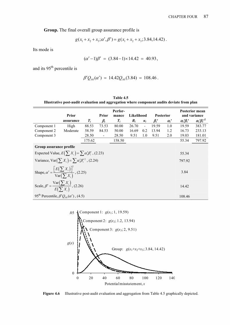
CHAPTER FOUR 87
Group. The final overall group assurance profile is
1 2 3 1 2 3( ; , ) ( ;3.84,14.42)g x x x g x x x .
Its mode is
( 1) (3.84 1) 14.42 40.93 ,
and its 95th percentile is
.95 .95( ) 14.42 (3.84) 108.46Q Q .
Table 4.5 Illustrative post-audit evaluation and aggregation where component audits deviate from plan
Prior PriorPerfor-mance Likelihood Posterior
Posterior mean and variance
assurance Ti i Ti Bi κi iʹ iʹ iʹiʹ iʹiʹ 2
Component 1 High 88.53 73.53 80.00 26.70 - 19.59 1.0 19.59 383.77 Component 2 Moderate 58.59 84.53 50.00 16.69 0.2 13.94 1.2 16.73 233.13 Component 3 28.50 - 28.50 9.51 1.0 9.51 2.0 19.03 181.01
175.62 158.50 55.34 797.92
Group assurance profile
Expected Value, i i iE X , (2.23) 55.34
Variance, 2Var i i iX , (2.24) 797.92
Shape,
2
Var
i
i
E X
X
, (2.25) 3.84
Scale,
Var i
i
X
E X
, (2.26) 14.42
95th Percentile, .95 ( )Q , (4.5) 108.46
Figure 4.6 Illustrative post-audit evaluation and aggregation from Table 4.5 graphically depicted.
0
.05
0 20 40 60 80 100 120 140
g(x)
Potential misstatement, x
Component 1: g(x1; 1, 19.59)
Component 2: g(x2; 1.2, 13.94)
Component 3: g(x3; 2, 9.51)
Group: g(x1+x2+x3; 3.84, 14.42)

88 THE GUAM METHOD FOR DETERMINING COMPONENT MATERIALITY
Group and component summary. The group and component distributions are depicted in
Figure 4.6. The group 95th percentile (108.46) exceeds group materiality of T = 100 and the group
auditor will need to consider whether this is acceptable or whether additional audit procedures are
required. It might be acceptable, for example, if “true” group materiality had been discounted in
anticipation of just such a result so that T = 100 actually represents group performance materiality
as discussed in Section 1.5.3.
4.5 Component materiality for a multilevel group
In the case of a multilevel group such as that depicted in Figure 2.6, it is first necessary to “flat-
ten” the group as depicted in Figure 4.7.so that the ultimate components can be correctly
weighted before component materiality is determined.
Although it may seem appealing at first, it is not valid to determine component materiality
in a stepwise manner. In Figure 4.7, for example, this would result in component materiality be-
ing determined for the three top level components, and then those component materialities being
used to determine component materiality at the next level, and so on. It can be readily seen, that
this approach will not result in the correct component materiality amounts. For example, if the
ultimate components are all identical, then this approach would result in greater component mate-
riality for higher level components than for lower level components, whereas component materi-
ality should be identical for identical components.44 The situation is different if a subgroup re-
quires a statutory audit. In that case, the subgroup materiality would be used in the determination
of component materiality for the subgroup’s components. As we saw in Section 2.5.3, the post
Structured seven-component group
Flattened seven-component group
Figure 4.7 “Flattening” a multilevel group before determining component materiality.
44 The requirement to “flatten” the group applies not only to GUAM but to other component materiality methods discussed in Chapter 5.
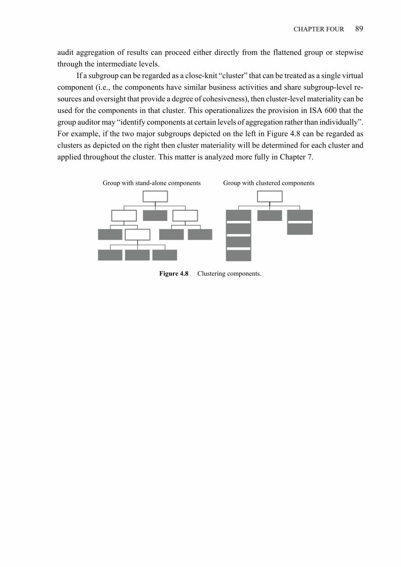
CHAPTER FOUR 89
audit aggregation of results can proceed either directly from the flattened group or stepwise
through the intermediate levels.
If a subgroup can be regarded as a close-knit “cluster” that can be treated as a single virtual
component (i.e., the components have similar business activities and share subgroup-level re-
sources and oversight that provide a degree of cohesiveness), then cluster-level materiality can be
used for the components in that cluster. This operationalizes the provision in ISA 600 that the
group auditor may “identify components at certain levels of aggregation rather than individually”.
For example, if the two major subgroups depicted on the left in Figure 4.8 can be regarded as
clusters as depicted on the right then cluster materiality will be determined for each cluster and
applied throughout the cluster. This matter is analyzed more fully in Chapter 7.
Group with stand-alone components Group with clustered components
Figure 4.8 Clustering components.


91
CHAPTER 5 Comparison of Component Materiality Methods
The choice of component materiality combination (T1, T2, …, TN) has a significant effect on overall
audit cost and achieved group assurance. This chapter develops measures of cost and achieved
group assurance; describes various alternatives to the GUAM method of materiality determina-
tion; and compares component materiality, cost, and achieved group assurance for GUAM and
the alternatives. Finally, the statistical bases of two alternatives to GUAM are analyzed and cri-
tiqued.
5.1 Alternative component materiality methods
This chapter compares the GUAM method with methods that represent the end points for compo-
nent materiality indicated by ISA 600, and with three other methods described in the literature
and used to some extent in global network firm practice. The five methods are:
MACM: Allocates maximum aggregate component materiality (a tabulated multiple of T)
to the components in proportion to the square root of size (Glover et al. 2008a).
SQRT: Sets Ti equal to T times the square root of the relative size of the component (Zuber
et al. 1983; Kinney 1993).
PROP: Allocates T to components in proportion to their size, the lower limit suggested by
ISA 600.
HALF: Sets Ti = T / 2 regardless of the number of components or component size (Kinney
1993).
FULL: Sets Ti = T for all components, the upper limit allowed by ISA 600.
Kinney (1993) also cites an audit manual used by some firms that recommends Ti = 0.75T. This
method is not included this in the study as it lies halfway between FULL and HALF. Formulas
for Ti under each of the methods are summarized in Table 5.1, both for the general case in which
the Yi are of variable size and for the special case in which they are identical. The formulas as-
sume negligible priors (adjusting for priors is described in Section 5.4.4). The table also summa-
rizes the formulas for relative total variable cost (RTVC), which is described in the next section.

92 COMPARISON OF COMPONENT MATERIALITY METHODS
Table 5.1 Summary of Ti and RTVC formulas for component materiality methods:
N components, negligible priors
Method Component materiality, Ti Relative total variable cost, RTVC*
General Yi Y1 =···= YN General Yi Y1 =···= YN
GUAM .95
.95
, 1(1/ ) i
i
TRw
Q w .95
.95 ( )
TR
Q N .95
.95
(1/ )i i
i
Y Q w
Y R
.95
.95
( )Q N
R
MACM† i
j
YmT
Y mT
N 2
i
i
Y
m Y
N
m
SQRT i
j
YT
Y
T
N
i
i
Y
Y
N
PROP i
j
YT
Y T
N N N
HALF 2
T
2
T 2 2
FULL T T 1 1
* Per equation (5.3). † From Glover et al. (2008a), a tabulated multiple m is applied to T giving maximum aggregate component materiality (MACM), which is allocated in proportion to the square root of size.The MACM multiples are as follows:
N 2 3-4 5-6 7-9 10-14 15-19 20-25 26-30
m 1.5 2.0 2.5 3.0 3.5 4.0 4.5 5.0
N 31-40 41-50 51-64 65-80 81-94 95-110 111-130 131+
m 5.5 6.0 6.5 7.0 7.5 8.0 8.5 9.0
5.2 Relative total variable cost of the group audit
To measure audit cost on a comparable basis, we assume that component audits entail a single
substantive test that is equivalent in information and cost to a misstatement-free MUS sample.
That is, we assume that component audit variable cost is proportional to the appropriate MUS
sample size. From (3.13), with Yi a proxy for relative total population size, sample size for Com-
ponent i is proportional to
.95
for 1,2, ,/
ii
i
Yn i N
T R .
While auditing standards do not require that statistical sampling be used, they do state that non-
statistical sample sizes will be similar or comparable to those derived statistically (ISA 530, para-

CHAPTER FIVE 93
graph A11). Thus MUS sample sizes are a convenient proxy for relative work effort and hence
for computing relative variable cost.45
If the variable cost per unit of auditing items in Component i is designated VCUi, then the
total variable cost for Component i is proportional to
.95 .95/ /
i i ii i i i
i i
Y VCU YTVC VCU n VCU
T R T R
. (5.1)
It follows from (5.1) that allowing VCUi to vary from component to component simply involves
replacing Yi with VCUi × Yi. Without loss of generality, therefore, we can eliminate the VCUi term
in (5.1) as long as we remember to bring it back when VCUi varies from component to compo-
nent. With this simplifying convention the total variable cost of auditing all N components is
.95/
ii
i
YTVC TVC
T R . (5.2)
By comparison, if the entire group (of size iY ) were treated as a “virtual single entity” and each
component audited using group materiality T (i.e., setting Ti = T for all i), then total variable cost
for the group would be minimized and would be proportional to .95/ /iY T R . Using this no-
tional minimum cost for a virtual single entity as the divisor, TVC is converted to a relative total
variable cost index (RTVC)
.95
.95
/ ( / ) /.
/ ( / ) /i i i i
i i
Y T R Y TRTVC
Y T R Y T
(5.3)
If Ti is constant across components, then
i
TRTVC
T . (5.4)
For example, for the case illustrated in Figure 4.3, (T1, T2) = (63, 63) and therefore RTVC =
100 / 63 = 1.58, or 58 percent more than if T were used throughout. For the case illustrated in Fig-
ure 4.4, (T1, T2) = (78, 63) and so
1/ 78 1/ 63
1.432 /100
RTVC
,
or 43 percent more than if T were used throughout. Thus, incorporating even a moderate group-
level prior for one component allows about a ten percent reduction in this group’s RTVC (from
1.58 to 1.43).
Because RTVC does not depend on the method used to determine (T1, T2, …, TN), equation
(5.3) provides a way to compare the cost implications of different component materiality meth-
45 Using the MUS sample size as a proxy for cost is equivalent to making the rough assumption that variable component audit cost is proportional to component size divided by component materiality.

94 COMPARISON OF COMPONENT MATERIALITY METHODS
ods. The formulas for RTVC under each of the alternative methods we consider are summarized
in Table 5.1.
5.3 Achieved group assurance
While GUAM-based component materiality combinations (T1, T2, …, TN) are constructed to ensure
AGA 95%, alternative component materiality methods may yield greater or lesser AGA. To
compare methods we assume that, regardless of how the group auditor determines component
materiality, the group auditor’s posterior component assurance profile for each component is
some exponential distribution ( ;1, )i ig x .46 Aggregating these posteriors via equations (2.27) and
(2.28) gives a group posterior of ( ; , )ig x , from which achieved group assurance is
( ; , )AGA G T .
If component priors are negligible then .95i iT R , therefore .95/i iT R , and from (2.27) and
(2.28),
2
2
2.95
( ; , ), where andi i
i i
T TAGA G T
T R T
. (5.5)
Equation (5.5) requires only (T1, T2, …, TN), and thus provides a way to calculate and compare
AGA for different methods assuming component priors are negligible. If the Ti’s are all equal then
(5.5) reduces to
1 .95 2 .95 .95( ; , ), where / / /NAGA G T N T R T R T R . (5.6)
For example, if T = 100 is allocated equally to two components so that (T1, T2) = (50, 50), then ʹ = N = 2, ʹ = 50 / 3.0, and AGA = G(100; 2, 50 / 3.0) = 98%.
5.4 Comparative analysis of component materiality, cost, and as-surance
In this section the alternative component materiality methods listed above are compared as to
Component materiality amount, Ti
Relative Total Variable Cost, RTVC, for the group
Achieved group assurance, AGA
While the comparison is limited to the alternatives considered in this thesis, it could be extended
to other methods that a firm or practitioner might consider. 46 An assumption that is implicit under ARM (see Section 3.3.2).

CHAPTER FIVE 95
5.4.1 Comparison for N identical components
Table 5.2 compares Ti, RTVC, and AGA for the component materiality methods listed in Section
5.1 for groups with two to ten components. Table 5.3 details the calculations for N = 3. Figure 5.1
charts Table 5.2.
Table 5.2 Comparisons of Ti, RTVC and AGA for 2 to 10 identical components
Component materiality
Ti Relative total variable cost
RTVC Achieved group assurance
AGA
N
GU
AM
MA
CM
SQ
RT
PR
OP
HA
LF
FU
LL
GU
AM
MA
CM
SQ
RT
PR
OP
HA
LF
FU
LL
GU
AM
MA
CM
SQ
RT
PR
OP
HA
LF
FU
LL
2 63 75 71 50 50 100 1.58 1.33 1.41 2.00 2.00 1.00 95% 91% 92% 98% 98% 80%
3 48 67 58 33 50 100 2.10 1.50 1.73 3.00 2.00 1.00 95% 83% 89% 99% 94% 58%
4 39 50 50 25 50 100 2.59 2.00 2.00 4.00 2.00 1.00 95% 85% 85% >99% 85% 35%
5 33 50 45 20 50 100 3.06 2.00 2.24 5.00 2.00 1.00 95% 71% 80% >99% 71% 18%
6 28 42 41 17 50 100 3.51 2.40 2.45 6.00 2.00 1.00 95% 72% 74% >99% 55% 8%
7 25 43 38 14 50 100 3.95 2.33 2.65 7.00 2.00 1.00 95% 55% 68% >99% 39% 3%
8 23 38 35 13 50 100 4.39 2.67 2.83 8.00 2.00 1.00 95% 55% 61% >99% 25% 1%
9 21 33 33 11 50 100 4.82 3.00 3.00 9.00 2.00 1.00 95% 54% 54% >99% 15% <1%
10 19 35 32 10 50 100 5.24 2.86 3.16 10.00 2.00 1.00 95% 35% 47% >99% 8% <1%
Table 5.3 Illustrative calculations: N = 3
Method Ti RTVC AGA
Table 5.1 Table 5.1 .95( , , / )iG T N T R , (5.6)
GUAM .95
.95 .95
100 3.0 30048
( ) (3) 6.3
TR
Q N Q
.95 .95
.95
( ) (3) 6.32.10
3.0 3.0
Q N Q
R (100,3,48 / 3.0) 95%G
MACM 2.0 100
673
mT
N
31.50
2.0
N
m (100,3,67 / 3.0) 83%G
SQRT 100
583
T
N 3 1.73N (100,3,58 / 3.0) 89%G
PROP 100
333
T
N N = 3 (100,3,33 / 3.0) 99%G
HALF 100
502 2
T 2 (100,3,50 / 3.0) 94%G
FULL T = 100 1 (100,3,100 / 3.0) 58%G

96 COMPARISON OF COMPONENT MATERIALITY METHODS
Componentmateriality
Ti
Relative totalvariable cost
RTVC
Achievedgroup
assurance
AGA
Number of components, N
Figure 5.1 Graphical depiction of comparisons in Table 5.2.
Overall, GUAM is consistently effective at lower relative cost than other effective methods
under these stylized conditions. It is the only method for which AGA = 95% is consistently
achieved. PROP is consistently more effective than GUAM (i.e., achieves AGA > 95%) and
HALF is more effective for N = 2. However, these are less efficient, incurring higher RTVC than
GUAM. The other alternatives are not effective in achieving AGA = 95%. Not surprisingly, their
RTVC is lower than for GUAM.
For reasons explained in Sections 1.5.2 and 4.1, the comparison is limited to ten and fewer
components, though it can easily be extended using the formulas, and there is no mathematical
limit. Figure 5.2 extends the Ti comparison to 256 components by powers of 2.
0
20
40
60
80
100
GUAM
MACMSQRT
HALF
FULL
PROP
1
2
3
4
5
MACM
PROP GUAM
SQRT
FULL
HALF
20%
40%
60%
80%
100%
2 3 4 5 6 7 8 9 10
FULL
PROP
SQRT
MACM
HALF
GUAM

CHAPTER FIVE 97
Figure 5.2 Ti Comparison for N = 2 to 256 equal-sized, identical components.
5.4.2 Asymptotic component materiality
Although the number of components in a group is seldom large, it is instructive to nevertheless
understand how component materiality behaves under the various methods in the theoretical cir-
cumstance that we have N identical components and N becomes large. The most conservative
method we have considered is PROP, where component materiality is inversely proportional to
the number of components, TPROP = T / N, which is a good proxy for the materiality amount that
would be appropriate if the component were a standalone entity being audited. In order to focus
just on differences between methods, we divide component materiality by TPROP, nominal stand-
alone materiality. In the case of GUAM, we have from (4.11) that component materiality is
.95
.95 ( )GUAM
TRT
Q N .
As a multiple of standalone component materiality it is
.95 .95 .95
.95
/ ( )
/ ( )GUAM
PROP
T TR Q N R N
T T N Q N .
For large N, we can replace Q.95(N) with the normal approximation (2.12)
.95 .95( )Q N N u N ,
to obtain
.95 .95
.95.95 1
GUAM
PROP
T R N RuT N u N
N
. (5.7)
0
10
20
30
40
50
60
70
80
90
100
2 4 8 16 32 64 128 256
Ti
N (Log2 scale)
HALF
FULL
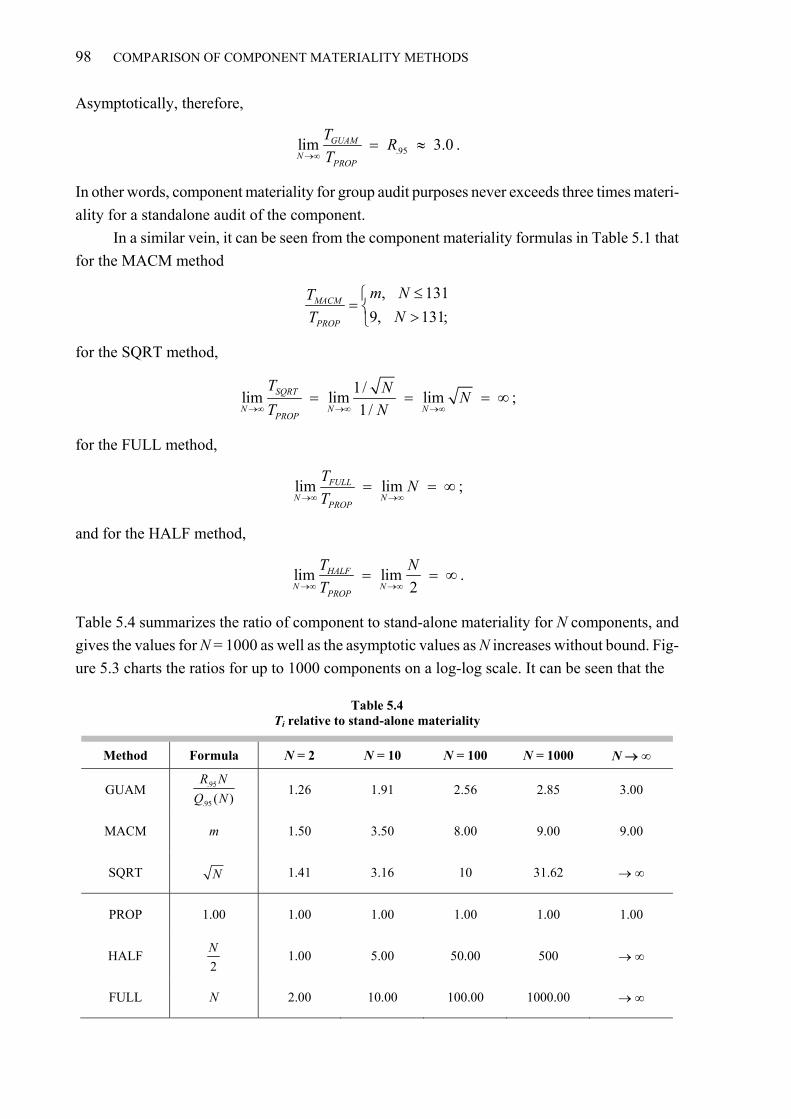
98 COMPARISON OF COMPONENT MATERIALITY METHODS
Asymptotically, therefore,
.95lim 3.0GUAM
NPROP
TR
T .
In other words, component materiality for group audit purposes never exceeds three times materi-
ality for a standalone audit of the component.
In a similar vein, it can be seen from the component materiality formulas in Table 5.1 that
for the MACM method
, 131
9, 131;MACM
PROP
m NT
NT
for the SQRT method,
1/
lim lim lim1/
SQRT
N N NPROP
T NN
T N ;
for the FULL method,
lim limFULL
N NPROP
TN
T ;
and for the HALF method,
lim lim2
HALF
N NPROP
T N
T .
Table 5.4 summarizes the ratio of component to stand-alone materiality for N components, and
gives the values for N = 1000 as well as the asymptotic values as N increases without bound. Fig-
ure 5.3 charts the ratios for up to 1000 components on a log-log scale. It can be seen that the
Table 5.4 Ti relative to stand-alone materiality
Method Formula N = 2 N = 10 N = 100 N = 1000 N ∞
GUAM .95
.95 ( )
R N
Q N 1.26 1.91 2.56 2.85 3.00
MACM m 1.50 3.50 8.00 9.00 9.00
SQRT N 1.41 3.16 10 31.62 ∞
PROP 1.00 1.00 1.00 1.00 1.00 1.00
HALF 2
N 1.00 5.00 50.00 500 ∞
FULL N 2.00 10.00 100.00 1000.00 ∞

CHAPTER FIVE 99
Figure 5.3 Ratio of Ti to TPROP,i.
GUAM ratio approaches 3, though rather slowly because the denominator in (5.7) involves the
square root of N; the MACM ratio ends at 9; the SQRT ratio is unbounded, though the increase is
much slower than HALF or FULL; and the PROP ratio is 1 by definition.
5.4.3 Illustrative comparison for unequal components
Table 5.5 compares methods for the illustrative three-component group, introduced in Table 4.1.
For comparability, assumptions include negligible priors, constant variable costs per unit across
components, and no externally imposed constraints on Ti, such as statutory audit requirements.
The GUAM calculations of Ti are detailed in Table 4.1. In this example, GUAM achieves AGA =
95% and RTVC = 1.87, while PROP achieves AGA > 95% at higher RTVC, and the other methods
achieve AGA < 95% at lower RTVC. HALF has higher RTVC and lower AGA than GUAM.
A comparison of RTVC in Table 5.5 with the N = 3 row in Table 5.3 illustrates a general
point, which is that costs are greatest when components are identical; for example, 2.10 in Table
5.2 versus 1.87 in Table 5.5. Identical components (an idealized extreme) therefore represents the
most conservative scenario.
Table 5.5 Illustrative Ti, RTVC, and AGA for nonidentical components, T = 100
Size(Yi) GUAM MACM SQRT PROP HALF FULL
Component materiality(Ti) Component 1 9,000 63 100 80 64 50 100 Component 2 4,000 48 67 53 29 50 100 Component 3 1,000 28 33 27 7 50 100
14,000 139 200 160 100 150 300
RTVC 1.87 1.29 1.60 3.00 2.00 1.00 AGA 95% 82% 91% 98% 94% 58%
1
10
100
1000
1 10 100 1000
Ratio (Log Scale)
N (Log Scale)
FULL
HALF
SQRT
MACM
GUAM
PROP

100 COMPARISON OF COMPONENT MATERIALITY METHODS
5.4.4 Inflating for priors—all methods
Although GUAM is the only method with an explicit formal process for incorporating prior as-
surance into the determination of component materiality, we can analyze the comparable effect of
prior assurance on alternative methods using the approach described in Section 4.3 for the
GUAM method.
Regardless of the method used to determine Ti, we can assume that components have asso-
ciated with them exponential priors, likelihoods and posteriors of the form g(xi; 1, i), g(xi; 1, Bi),
and g(xi; 1, iʹ) and that Ti is set at the 95th percentile of the target likelihood distribution, namely,
Ti = BiR.95. This is all that is required for the derivation of equation (4.17), which inflates compo-
nent materiality to account for prior assurance. It must be stated that there is nothing in the litera-
ture and no indication in practice that such adjustments are made, at least not on a formal basis.
Nevertheless, given the preceding assumptions, the inflation factors in Table 4.2 could be applied
regardless of the method. Table 5.6 illustrates the application of Table 4.2 across the different
methods for a two-component group. The first row shows Ti assuming negligible priors (i.e., iT )
and succeeding rows show Ti adjusted for prior assurance using the inflation factors in Table 4.2.
For example, for a moderate (50%) level of prior assurance, the inflation factor is 1.231 and the
MACM value of Ti is 1.231 × 75 = 92.
Table 5.6 Effect of priors on Ti
Prior Example: Ti for two-component group, Y1 = Y2, T = 100
Assur-ance
R Inflation
factor GUAM MACM SQRT PROP HALF FULL
0% 0.0 1.000 63 75 71 50 50 100 10% 0.1 1.035 65 78 73 52 52 104 30% 0.4 1.119 71 84 79 56 56 112 50% 0.7 1.231 78 92 87 62 62 123 70% 1.2 1.402 89 105 99 70 70 140 90% 2.3 1.769 112 133 125 88 88 177
5.5 Analysis of probabilistic alternatives
Since its publication in 2008, the MACM method has become quite widely used in practice. It is
analyzed in this section, as is the SQRT method proposed 25 years earlier.
5.5.1 The MACM method of Glover et al.
The MACM method for determining component materiality was proposed in an article in the De-
cember 2008 issue of Journal of Accountancy (Glover et al. 2008a) and some additional technical
details were published at the same time in an online supplement (Glover et al. 2008b). In the
MACM method a tabulated multiple m of group materiality called maximum aggregate compo-

CHAPTER FIVE 101
nent materiality (MACM) is allocated to significant components. The components are regarded as
N independent pass/fail Bernoulli trials in which each outcome is dichotomously either zero mis-
statement or misstatement exactly equal to some constant material amount, and m follows from
the binomial distribution. The multiple m (see Table 5.1) is a function of N, the number of signifi-
cant components to which MACM is allocated. Therefore,
MACM mT .
Certain fixed assumptions are built into the table regarding desired audit assurance at the compo-
nent and group levels. MACM is allocated to components in proportion to the square root of com-
ponent size,
ii
j
YT MACM
Y
,
and there are some rules of thumb to deal with conditions not well handled by the formula. In
email correspondence the authors indicated that the square root weighting allocation is styled af-
ter the formula used for the optimal allocation of total sample size to strata in stratified sampling,
so-called “Neyman allocation” (Cochran 1977, 98). It is formally the same as equation (4.6), the
formula for optimal weighting under the GUAM model.
The desired overall group assurance is P and 1−P is the acceptable audit risk at the group
level. The desired level of assurance at the component level is π and 1 − π is the acceptable audit
risk at the component level. For purposes of tabulating m, the authors assumed that P = 98%. The
article does not indicate what π is used for each entry, except that π = 95% for N = 5 and that π
ranges from 96% for small N (large components) to 90% for large N (small components).47
For the purpose of calculating m and hence MACM, it is assumed that the components are
identical and that component materiality is a constant TC = mT / N. It is also assumed that a com-
ponent either “fails”, in which case total misstatement for the component equals TC, or does not
fail, in which case component misstatement equals zero. The number of failed components is des-
ignated k, and kcrit is the critical number of failed components, that is kcritTC = T.
The model assumes that a component fails with probability 1−π and does not fail with prob-
ability π. The N components are regarded as N independent Bernoulli trials each with probability
of failure 1 − π. The probability of obtaining no more than k failures is given by the cumulative
binomial probability distribution,
0
Pr( ) (1 )k
i N i
i
Ni k
i
.
47 Note that in the GUAM method, there is not much point in specifying a different component assurance level. What matters is the form of the group auditor’s target likelihood function g(xi;1,Bi) and it is Bi that determines the extent of work. For given Bi, assurance and component materiality increase or decrease in tandem and the choice of what combination is specified is somewhat arbitrary.

102 COMPARISON OF COMPONENT MATERIALITY METHODS
In Excel this is
Pr( ) BinomDist( , ,1 , TRUE)i k k N cumulative .
More pertinent, however, is the number of failed components that can be tolerated con-
sistent with a group audit risk of 1 − P, or, more precisely, the smallest number of failed compo-
nents, such that the probability of having no more than that number amongst the N components is
at least P. This is the critical number of failed components kcrit. It can be found using the Excel
function
CritBinom( ,1 , )critk N P .
Given the assumptions in the model, group audit risk will be limited to no more than 1 − P if T =
TC × kcrit. Therefore, component materiality is set at TC = T / kcrit,
Ccrit crit
T NMACM NT N T
k k ,
and the multiple for N components is
crit
Nm
k . (5.8)
The example in the article assumes N = 5, 1 − π = 5%, and P = 98%. From these factors, the
critical number of failed components is
CritBinom(5,5%,98%) 2critk .
From (5.8),
5
2.52crit
Nm
k ,
which is the tabulated factor for N = 2 (see Table 5.1).
My criticism of the MACM model is that it is based on an unrealistic probabilistic represen-
tation of the actual auditing problem. It assumes that a component dichotomously fails or does not
fail and therefore Xi = TC or Xi = 0, and the factor m is based on identical components. It is more
realistic to represent component misstatement with a continuous random variable Xi to recognize
that there is a continuum of potential misstatement for each component and that component sizes
may vary, and to represent total group misstatement by iX . This is how the GUAM model rep-
resents the audit problem. In their technical description of the model, Glover et al. (2008b) recog-
nize these and other limitations of the MACM method noting that it, “…does not explicitly con-
sider the… risk that multiple components might contain undetected misstatements that are imma-
terial at the component level but aggregate to an amount that is material at the group level, or the
need for redistribution of materiality between components due to statutory audits or substantial
variability in the size of components.” The result of this simplification of the model is that nomi-
nal overall group assurance tends to be overstated as can be seen in Table 5.2 and Table 5.5.

CHAPTER FIVE 103
5.5.2 The SQRT method
The SQRT method (Zuber et al. 1983) is based on the Xi being independent normally distributed
random variables with mean zero and variance proportional to Yi. This leads to Ti equal to T times
the square root of the relative component size
ii
j
YT T
Y
(5.9)
(see Table 5.1). Although the authors do not explain their reasoning, a supporting argument
would likely go along the lines described in the following discussion.
Each component of size Yi dollars can be conceptualized as a population of Yi one-dollar
items on which are defined independent and identically distributed random variables xj (−∞, ∞),
j = 1, 2, …, Yi representing misstatement of item j (positive or negative) such that E(xj) = 0 and
Var(xj) = 2. Total component misstatement for Component i is therefore
1
iY
i jj
X x
with
2
1 1
( ) ( ) 0 and Var( ) Var( )i iY Y
i j i j ij j
E X E x X x Y
.
For the group as a whole, if1
N
iiX X
, then, because the Xi are independent,
2
1 1 1
( ) ( ) 0 and Var( ) Var( )N N N
i i ii i i
E X E X X X Y
.
By the Central Limit Theorem, the Xi and X are approximately normally distributed. As with
GUAM, Ti and T are 95th percentiles. For normal distributions centered on zero,
.95i iT u Y ,
where u.95 is the 95th percentile of the standard normal deviate. Similarly,
.95 iT u Y .
Therefore,
.95
.95
ii
j
u YT
T u Y
,
from which
ii
j
YT T
Y
,
which is SQRT formula (5.9).
104 COMPARISON OF COMPONENT MATERIALITY METHODS
The problem with this method is that it uses the normal distribution centered on zero to rep-
resent the auditor’s belief about total misstatement. As indicated in Section 2.1.1, because total
misstatement at the financial statement level is to be compared with a positive amount T, it too
must be a positive amount. In other words, the Xi’s should be positive valued random variables.
Blokdijk et al. (1995, 108) also criticize the SQRT method for its normal distribution basis
though their criticism is based more on sampling theory than on a Bayesian interpretation of the
underlying random variables.
5.6 Summary of comparative analysis
The comparative analysis in this section compares the Ti values delivered by each method and the
resulting RTVC and AGA. The RTVC calculation does not assume any underlying probabilistic
model, whereas the AGA calculation assumes component posterior assurance profiles are appro-
priately represented by exponential distributions, which, as noted earlier, is the implicit assump-
tion in ARM. GUAM delivers AGA = 95% by design, whereas the other methods deliver AGA <
95%, except for PROP which delivers AGA > 95%. In the sense of achieving the group audit as-
surance objective, therefore, GUAM and PROP are the only consistently effective methods.
PROP, however, is inefficient. The methods MACM, SQRT, FULL, and HALF have lower costs
than GUAM, but are ineffective.
The GUAM, MACM, and SQRT methods have probabilistic bases. All three assume sepa-
rate stand-alone components and stochastically independent Xi’s. The MACM and SQRT meth-
ods have probabilistic bases that are not well suited to the problem.
105
CHAPTER 6 Approximations and Optimizations
This chapter provides technical support for approximations and optimizations that were men-
tioned but glossed over in previous chapters. It can be skipped on a first reading.
Section 2.5 dealt with the convolution of gamma distribution, a function that is required for
the critical task of aggregating assurance across components. In general, the convolution of gam-
ma distributions with varying scale parameters is complex and in the GUAM model we approxi-
mate it with another gamma distribution. This chapter discusses the accuracy of the approxima-
tion.
Section 4.2.1 explained that the GUAM component materiality algorithm involves assign-
ing weights summing to 1 to components and plugging those weights into a formula to derive tar-
get component posteriors and hence component materiality amounts. This chapter shows that tar-
get component posteriors derived in this manner will aggregate to a group assurance profile that
meets group assurance objectives regardless of the weights that are assigned.
Section 4.2.2 stated that total group audit costs will be minimized when component are
weighted approximately in proportion to the square root of component size. This chapter derives
the square root formula.
Section 4.3 noted that while group auditor prior assurance about a component reduces com-
ponent audit cost, there is a cost to the group auditor who must expend effort in establishing and
supporting that prior assurance. A hypothetical example is used to illustrate how an optimal prior
might be established.
6.1 Approximating the convolution of gamma distributions
We consider the random variable X = X1 + X2 + ⋯ + XN where the Xi are independently distributed
as g(i, i). The distribution of X is the convolution of the N distributions g(xi; i, i). When the
i’s are equal the convolution is simply the gamma distribution ; ,ig x . The general case
of unequal i’s is quite complicated and has received special attention in the recent literature,
fueled in part by a surge in Bayesian applications and the availability of necessary computer
power. Just how complicated can be seen from the expression that Sim (1992) gives for the prob-

106 APPROXIMATIONS AND OPTIMIZATIONS
ability density function of the convolution:
11 1
1
( )1 1 1
1( )0
1( ; , , , , , ) exp
( )
( )( ) ,
!
i
N
N N ii N
rrN N
N Nrr N
xf x x
b rx
r
(6.1)
where
1
N
ii
,
and, for r = 0, 1, 2, …,
( ) ( )
( )r k
kk
r
and
( )1 2
( )0 1
1, 2,
( ) ( ) ( ), 3, 4, , ,
!
j jri i i j
ijj i
i
b r b j rc i N
j
and, finally,
1 12 11 1
1
i ii
i i
c
(Johnson et al. 1994; Stewart et al. 2007).
Because the convolution is expressed as an infinite sum and only a finite number of terms
can be calculated, some rounding error is unavoidable. More recently, Akkouchi (2005) ex-
pressed the cumulative distribution function as a multiple integral but the numerical solution also
leads to small rounding errors. Simulation is another method to find the nearly-exact convolution,
and great precision can be achieved very fast. If the convolution is an end in itself, these semi-
exact methods are quite satisfactory. If the convolution is just a step in a continuing argument,
however, a simple closed expression to approximate the convolution is more useful than a numer-
ical method, even at the cost of a slightly greater approximation error. Keeping the argument
within the family of gamma distributions also brings many analytical advantages to a model.
As we saw in Section 2.5.1, the GUAM model approximates the convolution with a gamma
distribution with the correct expected value and variance. Figure 6.1 shows an example based on
the three components in Table 4.4 where we have three independent gamma distributed random
variables, X1 ~ g(1, 21.08), X2 ~ g(1, 15.88), and X3 ~ g(1, 9.51). Because they do not have the
same scale parameter, their sum X = X1 + X2 + X3 has the non-gamma distribution described by
equation (6.1). That true distribution is approximated by the gamma distribution g(x; 2.74, 16.94)

CHAPTER SIX 107
computed in Table 4.4. In Figure 6.1 the true convolution is depicted as a solid curve, the approx-
imate convolution as a dotted curve. The two are practically identical.48
In our study (Stewart et al. 2007) my colleagues and I investigated the quality of the ap-
proximation, benchmarking it against the actual convolution. For computational efficiency we
used (6.1) as the actual probability density function, programming it in MATLAB and testing our
program against the Mathematica implementation of the convolution. We obtained cumulative
probabilities using numerical integration. We studied shape parameters ranging from 0.1 to 50
and scale parameters that differ by factors of up to ×10.
Our study shows that the approximation is highly accurate within the studied range; that it
is particularly good around the upper percentiles (e.g., the 95th), which is the region of most inter-
est to auditors; and that it tends to improve as N (the number of components) increases. When all
the component distributions are exponentials, as we assume for audit planning purposes, the true
confidence level at the nominal 95th percentile is no less than 94.9%. Therefore, the approxima-
tion overstates the level of confidence by no more than 1 / 1000 at the 95th percentile. Expressed
in terms of iX , the approximation understates the true 95th percentile by no more than 1 / 200.
That is, if the approximation indicates that 100 is the 95th percentile, the true percentile will be
between 100 and 100.5.49 In summary, using the gamma approximation instead of the true convo-
lution makes no appreciable difference to the final result while being much easier to implement
for practical field usage for any group likely to be encountered in practice.
Figure 6.1 Convolution of three gamma distributions F(x) (solid line) approximated by a gamma distribution G(x) (dotted line) with same mean and variance (CDFs).
48 In this example, I simulated the actual distribution of X = X1 + X2 + X3 by generating 20,000 random observa-tions (x1, x2, x3) for Xi ~ g(i,i) and x1 + x2 + x3. The simulation was performed in Excel and the percentiles were computed using the Percentile function. 49 This discrepancy can reasonably be regarded as insignificant, but an auditor who is concerned about it could reduce T to T / 1.005—using 99.5 instead of 100, for example.
0
1
0 20 40 60 80 100 120 140
G(x)F(x)
x = x1 + x2 + x3

108 APPROXIMATIONS AND OPTIMIZATIONS
Note on the scale parameter range in the Stewart et al. study
The Stewart et al. study includes scale parameters that differ in size by up to ten times. As shown
below this translates into component size differentials of at least 100. For the reasons given in
Section 1.5.2, it is unlikely that the group auditor would need to determine separate component
materialities or assurance profiles for components comprising less than 1% of the group.
Suppose, that there are N exponential posterior distributions with scale parameters i and
that k is K times the size of and l, that is, k = Kl, where K > 1. From (4.4) we have
.95 .95
and(1/ ) (1/ )k l
k l
T T
Q w Q w ,
and therefore
.95
.95
(1/ )
(1/ )k l
l k
Q wK
Q w
(6.2)
and
.95 .95(1/ ) (1/ )l kk
TQ w KQ w K
.
We show that if k / l equals K then the component weight ratio wk / wl exceeds K and approaches
K as k becomes smaller relative to T. Using approximation formula (2.13) and evaluating the
constant terms given P = 95% (which gives u.95 1.645), we have
2
2
10.142 0.822
41/
1/ 10.142 0.822
4
kk l
l k
k
TK
w w
w w T
. (6.3)
The relationship (6.3) between wk / wl and T / k is depicted in Figure 6.2 for K = 10 and T = 100.
It can be seen that the weight ratio wk / wl exceeds 10 (= K) and approaches K asymptotically and
rather slowly, which means that the weight ratio is significantly greater than K for most values of
interest.
The asymptotic approach can be confirmed analytically from (6.3). Expanding the terms in
(6.3) we have
1.645 0.142 0.784
1.645 0.142 0.784
k kk
l
k k
T TK K
w
w T T
.

CHAPTER SIX 109
Figure 6.2 Weight ratio wk / wl approaches 10 as k decreases while maintaining k = 10l.
As k approaches zero the numerator and denominator become very large and we may discard the
additive constants. Finally we divide top and bottom by T / k to get
0 0 0
1.645 1.645lim lim lim
1.645 1 1.645k k k
k
k kk
l k
k k
T TK K K K
w T Kw T T
T
.
Therefore, a scale differential of exactly ×K implies a weight differential of at least ×K.
with asymptotic equality. Translating weights into component size terms assuming that square
root weighting is used, we have
kk
l l
Yw
w Y ,
and therefore a weight differential of ×K implies a size differential of at least ×K 2. We have there-
fore shown that it takes a size differential of at least ×100 for the scale parameter differential to be
as large as ×10. For a two-component group, the size differential would have to be ×463.50
6.2 Achieving the group assurance objective
Section 4.2.1 stated without proof that under the GUAM method AGA 95% and ʹ Q.95(ʹ) T
(equation (4.5)) regardless of how components are weighted, provided they sum to 1. This section
analyzes the accuracy of the approximation.
50 This may be seen by substituting w2 = 1 − w1 in (6.2), which solves for (w1, w2) = (0.956, 0.044) giving Y1 / Y2 = (0.956 / 0.044)2 = 463.
10
15
20
1 10 100 1000
wk / wl
100 / k (log scale)

110 APPROXIMATIONS AND OPTIMIZATIONS
6.2.1 Approach and summary of results
Equation (4.5) can be rewritten as
.95 ( ) (1 )Q Err T . (6.4)
From equation (4.2), in the special case where components are equally weighted, wi = 1 / N, i = 1,
2, …, N, we have ʹ Q.95(N) = T and, accordingly, Err = 0. Up to a point, Err increases as the
weighting becomes more skew, and then decreases. Err also increases with N but at a decreasing
rate.
The behavior of Err was studied by simulating groups with 2 to 200 components of varying
size distributions. For each selected value of N between 2 and 200, 10,000 N-component groups
were simulated with components randomly selected from a suitably skew theoretical population.
The distribution approximates that which is known to characterize the distribution of firms within
the U.S. and other national economies. The simulation shows that even for N = 200 there is less
than one chance in a hundred that Err will exceed five percent of T.
Table 6.1 Detailed GUAM Ti calculations for Table 4.4 example but adjusting for Err
Component
1 2 3 4 5 6 7
Size √Size Weight Target
posterior
Component materiality (approx.)
Target posterior (error-
adjusted)
Component materiality
(error-adjusted)
iw i iT *
i *iT
iY iY i
j
Y
Y
.95 (1 / )i
T
Q w .95 (1)iQ
1i
Err
*.95 (1)i Q
Component 1 9,000 94.87 0.5000 21.0799 63.1496 21.0606 63.0920
Component 2 4,000 63.25 0.3333 15.8836 47.5831 15.8691 47.5397
Component 3 1,000 31.62 0.1667 9.5120 28.4954 9.5033 28.4694
14,000 189.74 1.0000 46.4755 139.2281 46.4331 139.1011
Group
Expected value, i iE X , (2.23) 46.4755 46.4331
Variance, 2Var i iX , (2.24) 787.1281 785.6924
Shape,
2
Var
i
i
E X
X
, (2.25) 2.7441 2.7441
Scale,
Var i
i
X
E X
, (2.26) 16.9364 16.9210
95th Percentile, .95 ( )Q , (4.1) 100.0913 100.0000
Error, .95 ( )Q TErr
T
, (6.4) 0.000913 −
Error correction factor,1 Err 1.000913 1.000000

CHAPTER SIX 111
In the simulation, the largest value of Err was 0.0566 and it was observed in one of the
10,000 simulated 200-component groups. Because Err tends to increase with group size and
groups with as many as 200 components for which component materiality is established are high-
ly unusual, we may conclude that Err will virtually never be greater than 6 percent of T. In prac-
tice, Err is small enough to be ignored. However, because Err depends only on the wi, it can be
computed ex ante and the error caused by the use of unequal weights can be eliminated by substi-
tuting T / (1 + Err) for T in equation (4.1). Therefore, using T / 1.06 instead of T would more than
compensate for Err in virtually all cases. Table 6.1 shows the GUAM calculation for the example
in Table 4.1 showing both the initial computation of Ti and error-adjusted *iT . Columns 1-3 con-
tain the optimal weight calculations per equation (4.6), Column 4 is the i calculation per equa-
tion (4.4), and Column 5 is Ti computed per equation (4.10). The aggregate group calculations
(lower panel) show that for this first iteration the group 95th percentile exceeds target group mate-
riality by 0.000913T. Columns 6 and 7 show the error-adjusted values of Columns 4 and 5, re-
spectively. The error-adjusted group calculations show that in this second iteration the group 95th
percentile = T and Err = 0. The miniscule value of Err observed in this example is consistent with
the overall results of the simulation study summarized above and described below.
6.2.2 Group simulation
It is well established that power laws describe the distribution of firm sizes within economies
(Gibrat 1931; Axtell 2001; Growiec et al. 2007; Pérez-Mesa and Galdeano-Gómez 2009) as well
as many other socioeconomic and naturally occurring quantities including city population sizes,
occurrence of natural resources, stock price fluctuations and personal incomes (Johnson et al.
1994, 607). Axtell (2001) analyzed U.S. Census Bureau data on the entire population of tax-
paying firms in the United States (some 5.5 million firms in 1997) and found that a simple power
law, the Zipf distribution, a discrete form of the long-tailed continuous Pareto distribution, char-
acterizes firm sizes. Zipf’s simple power law is one of the most striking empirical laws in eco-
nomics, describing a remarkably stable regularity in the spatial structure of market economies ap-
plying not only to the size of firms but also that of cities (Krugman 1996). It is reasonable to sim-
ulate N-component groups with samples of N from the Zipf distribution. If anything, randomly
selecting components from a simulated population of all firms in the economy will tend to result
in simulated groups with greater skewness in component sizes than one would expect in reality.
A Pareto probability distribution was used to construct a stylized universe of possible
groups. It is a “fat-tailed extended exponential” distribution that approximates the Zipf distribu-
tion and is often used to describe the distribution of economic data (Johnson et al. 1994, 607).
The original form of the Pareto distribution is
minmin min( ) Pr( ) , where 0, 0,
ay
F y Y y y a y yy
, (6.5)

112 APPROXIMATIONS AND OPTIMIZATIONS
where ( )F y is the probability that the random variable Y representing size (revenues, say) is great-
er than or equal to y, and ymin represents some minimum size (Johnson et al. 1994, 574). The
power a is a shape parameter. From (6.5) it follows that the cumulative distribution function may
be written as
min( ) 1a
yF y
y
. (6.6)
For a large universe the discrete Zipf distribution is well approximated by the (continuous)
Pareto distribution (6.6) with a = 1 and this approximation was used to model the distribution of
components. Since we are interested in relative rather than absolute sizes of components within
groups ymin was set to 1, reducing (6.6) to
1
( ) 1 , 1F y yy
. (6.7)
A stylized universe of N-component groups was thus created in which the sizes of each group’s N
components are the values of N random variables distributed as (6.7). The inverse transform sam-
pling method was applied to generate Pareto-distributed component sizes (Law 2007, 424), using
the inverse of (6.7),
1
1 ( )y
F y
.
If u is uniformly distributed on [0,1) then the random variable
1
1y
u
is distributed on [0,) as (6.7). Selecting an N-component group at random from the stylized uni-
verse of groups is simulated by generating N such Pareto-distributed random numbers.
Simulation results for groups with ten components
For illustrative purposes, Figure 6.3 shows the first ten of 10,000 groups randomly selected from
the universe of 10-component groups. Each group was synthesized by evaluating ten random var-
iables from equation (6.7). For each group relative component sizes are charted in descending or-
der. Reflecting reality, the sample of 10,000 includes a wide range of size distributions including
some very skew groups. Including highly-skewed groups in the study (which is what the Pareto
distribution ensures) is important because Err tends to increase with skewness. (For a totally flat
group with equal component sizes, Err = 0.) Table 6.2 shows in detail the calculation of Err for
one of the 10,000 selected 10-component groups.

CHAPTER SIX 113
Relative
component
size
For each group chart, Components 1 to 10 in decreasing order of size
Figure 6.3 Random selection of ten 10-component groups from a stylized universe.
Table 6.2 Illustrative calculation of Err for a 10-component group
Figure 6.4 depicts the cumulative frequency distribution of Err across all 10,000 groups
sampled from the stylized universe of 10-component groups. The median value of Err is 0.24%,
the 99th percentile is 1.26%, and the maximum value obtained is 1.37%. There is a 1% risk that
Err will exceed 1.26% for a group chosen at random. Taking this cumulative frequency curve as
an approximation of the cumulative probability distribution of Err across the stylized universe of
all 10-component groups leads to the conclusion that the risk that Err would exceed 5% is vanish-
ingly small.51 51 The distribution of Err for 10-component groups is quite closely approximated by the lognormal distribution. The fit is not as good for large groups however.
0.0
0.5
1.0
0.0
0.5
1.0
0.0
0.5
1.0
0.0
0.5
1.0
0.0
0.5
1.0
0.0
0.5
1.0
0.0
0.5
1.0
0.0
0.5
1.0
0.0
0.5
1.0
0.0
0.5
1.0
.5
.5
0
0
Y √Y w β' β' 2
1 0.4311 0.6566 0.2451 12.7121 161.5966 T 100.0000 2 0.2416 0.4916 0.1835 10.2379 104.8137 α' 8.0718 3 0.1000 0.3163 0.1181 7.2711 52.8686 β' 7.5806
4 0.0670 0.2588 0.0966 6.1939 38.3650 β'Q .95(α' ) 100.3744
5 0.0447 0.2114 0.0789 5.2530 27.5942 Err 0.3744%
6 0.0408 0.2020 0.0754 5.0605 25.6087 7 0.0282 0.1680 0.0627 4.3434 18.8652 8 0.0166 0.1289 0.0481 3.4716 12.0519 9 0.0152 0.1235 0.0461 3.3472 11.2041
10 0.0147 0.1213 0.0453 3.2977 10.8749 1.0000 2.6783 1.0000 61.1884 463.8429
Group
0
.5

114 APPROXIMATIONS AND OPTIMIZATIONS
Figure 6.4 Approximate cumulative distribution of Err for 10-component groups.
Simulation results for groups with 2 to 200 components
Table 6.3 summarizes the results of the simulation for groups with up to 200 components show-
ing the median, 99th percentile and maximum obtained values of Err. Results for each N are based
on a random sample of 10,000 N-component groups from a stylized universe of groups using rela-
tive square root weighting
ii
j
Yw
Y
.
The results demonstrate that the risk is less than 1% that Err will exceed 5% for N up to 200 for a
group chosen at random from the stylized universe. The results are depicted graphically in Figure
6.5.
To further test the possible distribution of Err the simulation described above was rerun us-
ing the simplistic direct weighting formula
ii
j
Yw
Y
,
which leads to weight distributions more skewed than in the first simulation (which is flattened
by the square root formula). The results are tabulated in Table 6.4 and depicted in Figure 6.6.
While the median values of Err were greater than those indicated in Table 6.3, the 99th percentiles
were not much greater and none (up through N = 200) exceeded 5%. The results demonstrate that
the risk is less than 1% that Err will exceed 5% for N up to 200.
0
0.5
1
0.0 0.2 0.4 0.6 0.8 1.0 1.2 1.4
Frequency
Err Percent
99th Percentile = 1.26
Median = 0.24

CHAPTER SIX 115
Table 6.3 Err percent, relative square-root weights
Figure 6.5 Summary of simulations graphically de-picted—square-root weights.
Table 6.4 Err percent, proportional weights
Figure 6.6 Summary of simulations graphically de-picted—proportional weights.
6.3 Minimizing group audit costs
This section shows that square-root weighting formula (4.6) introduced in Section 4.2.2 yields
weights and hence component materiality amounts that minimize total cost.
6.3.1 Derivation of formula
From equation (5.2) and equation (4.9) total variable cost is
.95 .95
.95.95
(1/ ) / 1(1/ )i i i i
i i ii
R Y Q w T YTVC TVC YQ w
TR T
, (6.8)
where Yi is revenues, total assets, or some other appropriate financial benchmark. For the reason
noted in Section 5.2, allowing VCUi to vary from component to component simply involves re-
placing Yi in (6.8) with VCUi × Yi.
Minimizing TVC with respect to (w1, w2, …, wN) is a classic constrained optimization prob-
lem in which the goal is to find the weights that minimize the objective function
1 2 .95( , , , ) (1/ )N j jf w w w Y Q w
0
1
2
3
4
5
6
0 50 100 150 200
Err
Per
cent
N
Median
99th Percentile
Maximum
N Median99th
Percentile Maximum
2 0.02 0.28 0.295 0.10 0.73 0.7910 0.24 1.26 1.3720 0.43 2.01 2.1850 0.66 3.13 3.46
100 0.79 3.97 4.59200 0.82 4.43 5.66
0
1
2
3
4
5
6
0 50 100 150 200
Err
Perc
ent
N
Median
99th Percentile
Maximum
N Median99th
Percentile Maximum
2 0.06 0.29 0.295 0.29 0.77 0.7910 0.69 1.30 1.3620 1.20 2.02 2.1750 1.93 3.09 3.40
100 2.46 3.88 4.22200 2.97 4.62 5.20

116 APPROXIMATIONS AND OPTIMIZATIONS
subject to the constraint 1jw .52 Following the Lagrange method (Cooper and Steinberg 1970,
120), we construct
1 2 .95( , , , , ) (1/ ) 1N j j jF w w w Y Q w w ,
differentiate it with respect to the wi and λ, and set the partial derivatives equal to zero, thus ob-
taining the equations
.95
1 2 2
1 2
(1/ )( , , , , ) 0 for 1, 2, , , and
( , , , , ) 1 0,
i
i iw N
i
N j
YQ wF w w w i N
w
F w w w w
where Q′.95 is the derivative of Q.95 with respect to 1 / wi and F′ is the partial derivative of F with
respect to the subscripted variable. Solving for wi gives
.95
.95
(1/ )
(1/ )i i
i
j j
YQ ww
Y Q w
. (6.9)
Solution (6.9) is easily shown to minimize not maximize the objective function.
Because (6.9) involves the derivative of the percentile function, which involves wi, it cannot
be solved explicitly for wi but requires an iterative solution. Fortunately, the derivatives make no
appreciable difference and can be ignored, thus leading to
ii
j
Yw
Y
, (6.10)
justification for which now follows.
6.3.2 Justification for ignoring derivative terms
First, it should be noted that both (6.9) and (6.10) result in weights that sum to 1 and therefore
both result in component materiality amounts that meet group assurance objectives. The worst
that can happen if the simpler formula is used is that the weighting is somewhat sub-optimal from
a cost perspective. Here we justify regarding the degree of sub-optimization as insignificant.
Because there is no closed form expression for the percentile function, we differentiate the
approximating function (2.11) with respect to to get
22 .95
.95 .95 .95
1 1( ) 4 1 1 1
4 12 4 1
udQ a u a u
d a
,
52 The objective function is equation (6.8) with the constant terms eliminated.

CHAPTER SIX 117
and therefore
.95.95 (1/ ) 1
4 / 1i
i
uQ w
w
is the derivative of Q.95 with respect to 1 / wi. From this we see that
.950lim (1/ ) 1
ii
wQ w
and
.951
1.6448...lim (1/ ) 1 1.95
3.0ii
wQ w
.
Because Q′.95 is a monotonically increasing function of wi on (0,1), it varies between a minimum
value of 1 and a maximum value of 1.95. Therefore, .95 (1/ )iQ w , the term that enters (6.9), varies
between 1 and √1.95 = 1.4. Because of its narrow range, because it increases monotonically with
iY , and because the product .95 (1/ )i iYQ w appears in both the numerator and the denominator,
including .95 (1/ )iQ w in (6.9) does not make a significant difference and, accordingly, (6.10) is a
good approximation to (6.9).
Consider the example in Table 4.1. The weights based on simplified formula (6.10) are
(w1, w2, w3) = (0.5000, 0.3333, 0.1667) and the resulting component materiality combination is
(T1, T2, T3) = (63.15, 47.58, 28.50). If derivatives are included, then, after four iterations of (6.9),
the weights converge to (w1, w2, w3) = (0.5159, 0.3288, 0.1552) and the corresponding component
materiality combination is (T1, T2, T3) = (64.52, 47.12, 26.98).
The iterative calculation is shown in Table 6.5. The initial weights in Iteration 1, are those
calculated per simplified equation (6.10). In Iteration 2 those weights are used as input to the
right-hand side of (6.9) and new weights are calculated. After Iteration 4 the weights have con-
verged to four decimal places.
Translated into cost terms, weighting (6.10), which ignores derivatives, gives
9000 / 63.15 4000 / 47.58 1000 / 28.50
1.869114000 /100
RTVC
,
whereas weighting (6.9), which includes derivatives, gives
9000 / 64.52 4000 / 47.12 1000 / 26.98
1.867514000 /100
RTVC .
From this we deduce that the “relative inefficiency” of the simplified weighting is
1.8691
1 1 0.000871.8675
RTVC
RTVC
,
or less than 1 / 1000.

118 APPROXIMATIONS AND OPTIMIZATIONS
Table 6.5 Illustrative iterative calculation of component weights
Process Component 1 Component 2 Component 3 Total
Y 9,000 4,000 1,000 14,000 √Y 94.8683 63.2456 31.6228 189.7367 w 0.5000 0.3333 0.1667 1.0000
Equation (4.10)/(6.10) Ti 63.15 47.58 28.50 139.23 Iteration 1 w 0.5000 0.3333 0.1667 1.0000
√Q' 1.2735 1.2231 1.1589 3.6554 √YQ' 120.8109 77.3548 36.6466 234.8123
Iteration 2 w 0.5145 0.3294 0.1561 1.0000 √Q' 1.2775 1.2218 1.1539 3.6531 √YQ' 121.1924 77.2728 36.4888 234.9540
Iteration 3 w 0.5158 0.3289 0.1553 1.0000 √Q' 1.2778 1.2216 1.1535 3.6530 √YQ' 121.2268 77.2612 36.4772 234.9652
Iteration 4 w 0.5159 0.3288 0.1552 1.0000 √Q' 1.2779 1.2216 1.1535 3.6529 √YQ' 121.2300 77.2598 36.4763 234.9662
Iteration 5 w 0.5159 0.3288 0.1552 1.0000
Equation (4.10)/(6.9) Ti 64.52 47.12 26.98 138.62
Figure 6.7 shows the relative inefficiency of the simplified square-root weighting formula
for two-component groups. The horizontal axis is the relative size of Component 1 (the relative
size of Component 2 is its complement). The chart confirms that relative inefficiency is mini-
mal—less than 2.5 / 1000—regardless of how skew the group is, and approaches that maximum
only for highly skew groups where one component is in the region of 3% (or 97%) of the group.
For equal size components the weights are (0.5,0.5) under both formulas and so there is no ineffi-
ciency. Inefficiency also disappears asymptotically for extremely skewed groups.
Figure 6.7 Relative inefficiency of simplified square-root weighting for two-component groups.
0
.0005
.0010
.0015
.0020
.0025
0 .1 .2 .3 .4 .5 .6 .7 .8 .9 1.0
Inefficiency of simplified weighting
Relative size of Component 1

CHAPTER SIX 119
6.4 Optimizing priors: a hypothetical illustration
As noted in Section 4.3, there is potential for a tradeoff between the cost of the group auditor es-
tablishing or strengthening prior component assurance to increase component materiality and the
resulting reduction in component auditor cost. An economically optimal component prior is one
that minimizes total cost. I am not aware of any cost function for computing the cost of establish-
ing a component prior so this discussion is hypothetical and its purpose is simply to illustrate the
kind of relationship that might plausibly exist.
Let us assume that the size of Component i is Yi and that the target exponential posterior
assurance profile g(xi; 1, iʹ) has been established for the component, where, per equation (4.4),
.95 (1/ )i
i
T
Q w .
The group auditor needs to decide how much to spend on establishing an exponential prior assur-
ance profile g(xi; 1, i) for the component in order to increase component materiality and thus re-
duce component auditor cost. Component auditor variable cost is a function of the required likeli-
hood distribution g(xi; 1, Bi) where, per (4.7),
1
, where 01/ 1/i i i
i i
B
.
As discussed in Section 5.2, we may assume as a rough rule of thumb that component auditor cost
(CAC) is proportional to the sample size that would result from applying MUS to the component.
Per (3.12), that is, proportional to
ii
i
YCAC K
B
for some constant Ki. Writing this as a function of i gives
1 1
( ) , where 0i i i i ii i
CAC K Y
.
Let us assume for the purposes of this discussion that the group auditor cost (GAC) of es-
tablishing the component prior g(xi; 1, i) is a power function of i,
( ) , where , 0 and 1idi i i i i iGAC c c d .
In this power function the negative exponent reflects that the cost of establishing a very tight prior
(small i) would be high, tending asymptotically to infinity (at least in theory) as i tends to zero
and that cost decreases but at a declining rate as i increases.
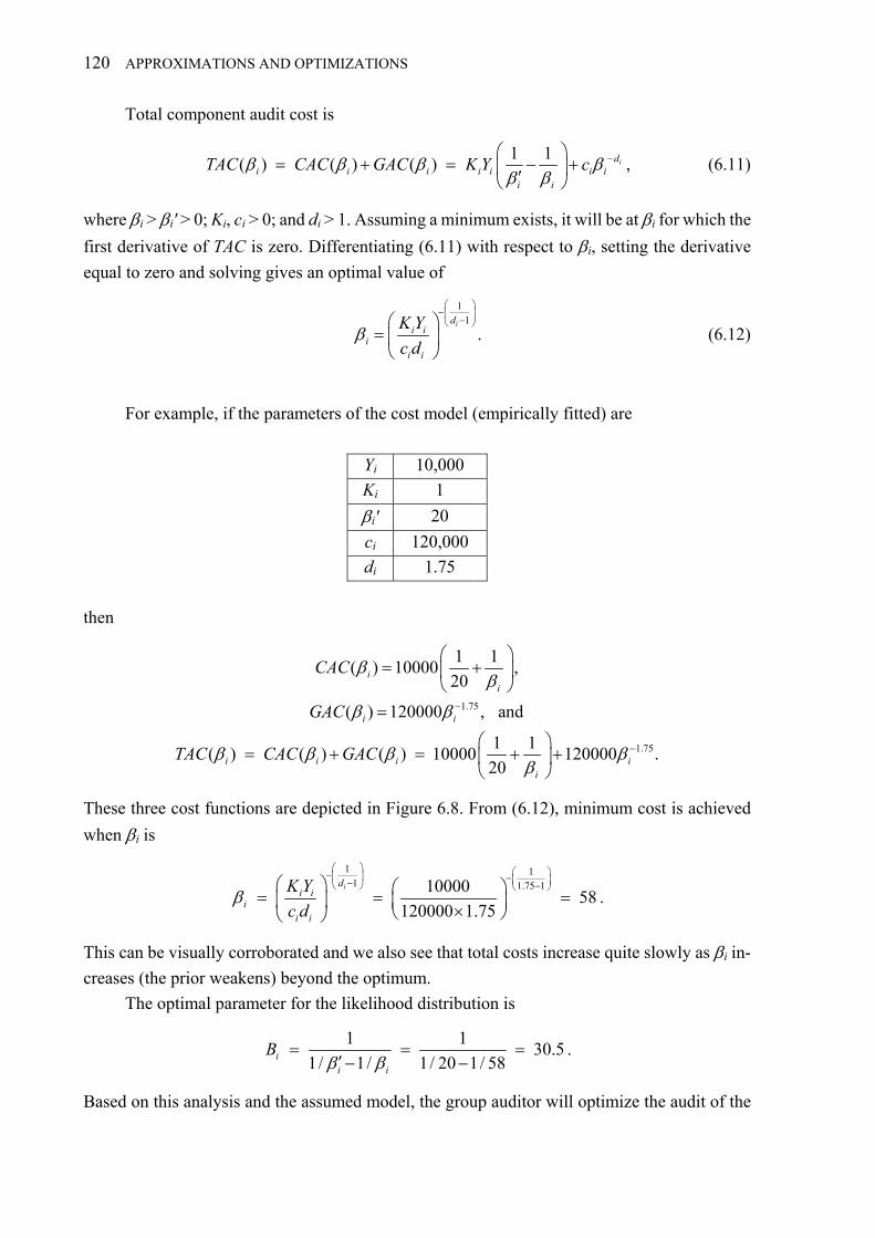
120 APPROXIMATIONS AND OPTIMIZATIONS
Total component audit cost is
1 1
( ) ( ) ( ) idi i i i i i i
i i
TAC CAC GAC K Y c
, (6.11)
where i > iʹ > 0; Ki, ci > 0; and di > 1. Assuming a minimum exists, it will be at i for which the
first derivative of TAC is zero. Differentiating (6.11) with respect to i, setting the derivative
equal to zero and solving gives an optimal value of
1
1idi i
ii i
K Y
c d
. (6.12)
For example, if the parameters of the cost model (empirically fitted) are
Yi 10,000
Ki 1
iʹ 20
ci 120,000
di 1.75
then
1.75
1.75
1 1( ) 10000 ,
20
( ) 120000 , and
1 1( ) ( ) ( ) 10000 120000 .
20
ii
i i
i i i ii
CAC
GAC
TAC CAC GAC
These three cost functions are depicted in Figure 6.8. From (6.12), minimum cost is achieved
when i is
1 11 1.75 110000
58120000 1.75
idi i
ii i
K Y
c d
.
This can be visually corroborated and we also see that total costs increase quite slowly as i in-
creases (the prior weakens) beyond the optimum.
The optimal parameter for the likelihood distribution is
1 1
30.51/ 1/ 1/ 20 1/ 58i
i i
B
.
Based on this analysis and the assumed model, the group auditor will optimize the audit of the

CHAPTER SIX 121
component by establishing prior assurance represented by g(xi; 1, i) with i = 58 and a likelihood
distribution g(xi; 1, Bi) with Bi = 30.5. The posterior will be g(xi; 1, iʹ) with iʹ = 20.
Because .95/i iT R and /ii i PT R , we have
.95
20
58iPi
i
R
R
,
from which
.95
20 203.0 1.03
58 58iPR R .
From (2.16), 1.03 = −ln(1 − Pi), and therefore
1.031 .64iP e .
This indicates that, from a cost perspective, the component auditor should ideally achieve prior
assurance of Pi = 64% (i.e., RMMi = 36%). In other words, based on this model and the scale in
Table 2.2, the group auditor ideally should aim at achieving moderate to high assurance.
Figure 6.8 Illustrative component auditor and group auditor component costs as a function of i.
0
100
200
300
400
500
600
0 20 40 60 80 100 120 140 160 180 200
Cost
Prior βi
Group Auditor GAC(βi)
Component Auditor CAC(βi)
Total TAC(βi)


123
CHAPTER 7 Optimizing for Group Context, Constraints, and Structure
This chapter shows how the GUAM component materiality algorithm adjusts for practical factors
encountered in group audits by locating optimal component materiality combinations that lie
along an efficient materiality frontier. It also shows how the auditor can leverage group structure
including group-wide controls to substantially reduce component audit cost.
7.1 Optimizing along the “Efficient Materiality Frontier”
We have seen that, in the absence of additional constraints, square-root weighting formula (4.6)
assigns optimal weights in the GUAM component materiality algorithm (see Sections 4.2.2 and
6.3). In practice, additional constraints on component materiality often lead to different optimal
weights. For example:
Component materiality may be constrained by statutory audit requirements, by specific user
expectations, or by the requirements of a jurisdiction-specific financial reporting frame-
work.
Audit costs may vary significantly between components.
A component may be easy to audit “one-hundred percent” thus effectively reducing com-
ponent audit risk to zero. 53
We have seen that the GUAM method delivers component materiality combinations that
meet the group audit assurance objective (AGA = 95%) regardless of how the components are
weighted, just as long as the weights sum to 1. Because there is a continuum of weight combina-
tions (w1, w2, …, wN) that sum to 1, there is a corresponding continuum of component materiality
combinations (T1, T2, …, TN) for which AGA = 95%. In the case of just two components this con-
tinuum can be depicted as a curve in the positive quadrant of the real plane. The EMF for N = 2, T
= 100, and negligible priors is depicted in Figure 7.1 (the curve labeled GUAM).
53 For example, a component may hold a small number of fixed investments that together with their income streams will be audited 100 percent.

124 OPTIMIZING FOR GROUP CONTEXT, CONSTRAINTS, AND STRUCTURE
Figure 7.1 Efficient materiality frontier: two components, negligible priors, T = 100.
The EMF partitions all possible component materiality combinations into two regions.
Those above the curve comprise the “region of ineffectiveness” as they do not meet the group as-
surance objective, that is AGA < 95%. It is a region characterized by underauditing. Those on or
below the curve comprise the “region of effectiveness” as they meet or exceed the group assur-
ance objective, that is, AGA ≥ 95%. While combinations strictly below the curve are effective,
they are also inefficient because they result in more audit work than is necessary to achieve 95%
assurance—and the inefficiency increases the closer the combination is to the origin. It is a region
characterized by overauditing. On the other hand, combinations exactly on the curve exactly
achieve the group assurance objective. We call this curve the efficient materiality frontier (EMF).
All GUAM-based combinations (T1, T2, …, TN) are constructed to lie on the EMF because they are
based on weight combinations (w1, w2, …, wN) assigned to components such that iw = 1. Deter-
mining optimal weighting subject to given constraints therefore consists of locating the compo-
nent materiality combination on the EMF determined by the constraints.
In addition to the EMF, Figure 7.1 also depicts the curves plotting (T1, T2) combinations for
MACM, SQRT and PROP and the fixed points corresponding to HALF and FULL. Note that the
FULL combination and all combinations using SQRT and MACM are above the EMF and thus
ineffective relative to GUAM, while all combinations using PROP are below the EMF and thus
effective, but inefficient relative to GUAM. Finally, for N = 2, HALF, like PROP, is effective but
inefficient. It needs to be emphasized that the EMF curve in Figure 7.1 assumes negligible priors.
As we will see, a different curve results if priors are non-negligible for either or both components.
Underauditing
Overauditing
EMF (GUAM)
0
10
20
30
40
50
60
70
80
90
100
0 10 20 30 40 50 60 70 80 90 100
T2
T1
FULL
(63,63)
(50,75)(48,77)
HALF
(0,100)
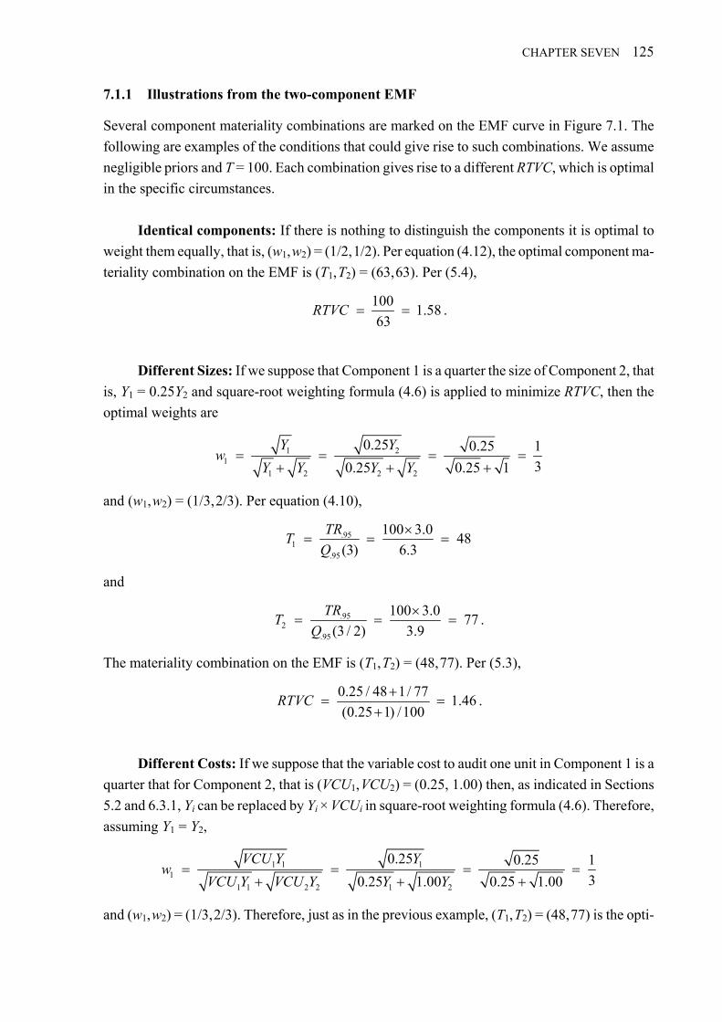
CHAPTER SEVEN 125
7.1.1 Illustrations from the two-component EMF
Several component materiality combinations are marked on the EMF curve in Figure 7.1. The
following are examples of the conditions that could give rise to such combinations. We assume
negligible priors and T = 100. Each combination gives rise to a different RTVC, which is optimal
in the specific circumstances.
Identical components: If there is nothing to distinguish the components it is optimal to
weight them equally, that is, (w1, w2) = (1/2, 1/2). Per equation (4.12), the optimal component ma-
teriality combination on the EMF is (T1, T2) = (63, 63). Per (5.4),
100
1.5863
RTVC .
Different Sizes: If we suppose that Component 1 is a quarter the size of Component 2, that
is, Y1 = 0.25Y2 and square-root weighting formula (4.6) is applied to minimize RTVC, then the
optimal weights are
1 21
1 2 2 2
0.25 0.25 1
30.25 0.25 1
Y Yw
Y Y Y Y
and (w1, w2) = (1/3, 2/3). Per equation (4.10),
.951
.95
100 3.048
(3) 6.3
TRT
Q
and
.952
.95
100 3.077
(3 / 2) 3.9
TRT
Q
.
The materiality combination on the EMF is (T1, T2) = (48, 77). Per (5.3),
0.25 / 48 1/ 77
1.46(0.25 1) /100
RTVC
.
Different Costs: If we suppose that the variable cost to audit one unit in Component 1 is a
quarter that for Component 2, that is (VCU1, VCU2) = (0.25, 1.00) then, as indicated in Sections
5.2 and 6.3.1, Yi can be replaced by Yi × VCUi in square-root weighting formula (4.6). Therefore,
assuming Y1 = Y2,
1 1 11
1 1 2 2 1 2
0.25 0.25 1
30.25 1.00 0.25 1.00
VCU Y Yw
VCU Y VCU Y Y Y
and (w1, w2) = (1/3, 2/3). Therefore, just as in the previous example, (T1, T2) = (48, 77) is the opti-

126 OPTIMIZING FOR GROUP CONTEXT, CONSTRAINTS, AND STRUCTURE
mal component materiality combination on the EMF, and RTVC = 1.46. This and the previous
example illustrate that each point on the EMF can be optimal for various scenarios.
Constrained component materiality: There are many reasons why component materiality
may be constrained to some amount less than that required for group audit purposes, the most
common being statutory audit requirements. The effect of constraining component materiality is
that more assurance is obtained than is required to satisfy the group auditor’s assurance objective.
Loosely speaking, the “excess” assurance obtained for constrained components may be offset by
relaxing the assurance objectives for the other components by increasing their component materi-
ality amounts. Under the GUAM method this is technically accomplished by computing the com-
ponent weights that are implied by each constrained component materiality amount and rebalanc-
ing the remaining component weights so that weights sum to 1 across the entire group.
Suppose that in our two-component group, Component 1 will be audited using T1 = 50, an
amount that is less than that required for group purposes. From (4.10), mandating T1 = 50 implies
an effective weight w1 that is the solution to
.95.95 1
1
100 3.0(1/ ) 6.0
50
TRQ w
T
. (7.1)
Solving for w1 (for example, by using the Excel Goal Seek tool) yields w1 = 0.36, and setting w2 =
1 − w1 gives (w1, w2) = (0.36, 0.64). Applying (4.10) again gives
1 2.95 .95
3.0 3.0100 50 and 100 75
(1/ 0.36) (1/ 0.64)T T
Q Q .
Therefore, (T1, T2) = (50, 75) is the optimal component materiality combination on the EMF. As-
suming the components are otherwise identical, (5.3) gives,
1/ 50 1/ 75
1.67(1 1) /100
RTVC
.
This approach to accommodating constrained component materiality can be generalized to multi-
ple components as explained in Section 7.2.2 below.
Zero risk component: Suppose that Component 1 is audited so thoroughly that audit risk is
effectively reduced to zero for that component. For example, if the component has a small num-
ber of readily verifiable assets with fixed and computable income streams, the component auditor
may be able to audit the component “100 percent”. Since we assume that any misstatements de-
tected in the audit of Component 1 are corrected to the satisfaction of the auditor, any remaining
misstatements are limited to Component 2. It is mathematically sufficient, therefore, to set T2 = T
for group audit purposes. Therefore, at the extreme, the optimal EMF component materiality pair
is (T1, T2) = (0, 100). Because it is assumed that Component 1 is audited 100 percent, the notion of
VCU does not apply to that component and RTVC is not computed. The extreme optimum, (T1, T2)
= (0, 100), is also approached as Y1 or VCU1 approach zero.

CHAPTER SEVEN 127
7.1.2 Adjusting the EMF for prior assurance
Figure 7.2 shows three two-component EMF curves to demonstrate the effect of introducing prior
component assurance. The negligible prior case is shown for reference purposes as EMF 0. This is
the same as the EMF curve in Figure 7.1. For example, the component materiality combination
for two otherwise identical components is (63, 63). The EMF 1 curve is for moderate prior assur-
ance for Component 1 and negligible prior assurance for Component 2. This is the situation re-
flected in Figure 4.4 where the component materiality combination for two otherwise identical
components is (78, 63), a combination that lies on EMF 1. In this case, per Table 4.2, T1 =
63 × 1.231 = 78. Where there is moderate prior assurance for both identical components, the ma-
teriality combination is (78, 78), which lies on EMF 2. In this case, per Table 4.2, T1, T2 =
63 × 1.231 = 78.The curves for MACM, SQRT and PROP are also shown in the background.
The shift in the EMF curve away from EMF 0 reflects the increase in component materiality
when priors are introduced and is governed by equation (4.18). As can be seen in Figure 7.2 it is
possible for component materiality to exceed group materiality. This condition is explained in
Section 4.3.2.
Figure 7.2 Two-component EMF with 0, 1, and 2 non-negligible priors.
7.2 Extending to N components
For N = 2 the EMF is represented by a convex curve in the positive quadrant exemplified by those
in Figure 7.1 and Figure 7.2. For N = 3 the EMF can be represented by an analogous two-
dimensional convex curved surface in the positive octant. For N > 3 the EMF is an N − 1-
dimensional convex hyper-curve in the positive hyper-quadrant and easy visualization is not fea-
sible. Nevertheless, the curve can be described mathematically and we can prove that the N − 1-
0
20
40
60
80
100
120
140
0 20 40 60 80 100 120 140
T2
T1
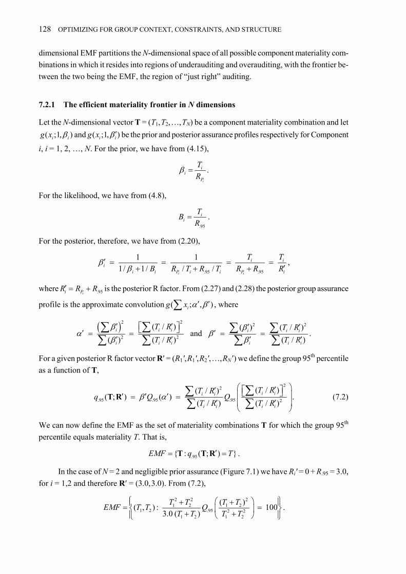
128 OPTIMIZING FOR GROUP CONTEXT, CONSTRAINTS, AND STRUCTURE
dimensional EMF partitions the N-dimensional space of all possible component materiality com-
binations in which it resides into regions of underauditing and overauditing, with the frontier be-
tween the two being the EMF, the region of “just right” auditing.
7.2.1 The efficient materiality frontier in N dimensions
Let the N-dimensional vector T = (T1, T2, …, TN) be a component materiality combination and let
( ;1, )i ig x and ( ;1, )i ig x be the prior and posterior assurance profiles respectively for Component
i, i = 1, 2, …, N. For the prior, we have from (4.15),
i
ii
P
T
R .
For the likelihood, we have from (4.8),
.95
ii
TB
R .
For the posterior, therefore, we have from (2.20),
.95 .95
1 1
1/ 1/ / /i i
i ii
i i P i i P i
T T
B R T R T R R R
,
where .95ii PR R R is the posterior R factor. From (2.27) and (2.28) the posterior group assurance
profile is the approximate convolution ( ; , )ig x , where
22
2 2
2 2
( / ) ( ) ( / )and
( ) ( / ) ( / )i ii i i i
i i i i i i
T R T R
T R T R
.
For a given posterior R factor vector Rʹ = (R1ʹ, R1ʹ, R2ʹ, …, RNʹ ) we define the group 95th percentile
as a function of T,
22
.95 .95 .95 2
( / )( / )( ; ) ( )
( / ) ( / )i ii i
i i i i
T RT Rq Q Q
T R T R
T R . (7.2)
We can now define the EMF as the set of materiality combinations T for which the group 95th
percentile equals materiality T. That is,
.95{ : ( ; ) }EMF q T T T R .
In the case of N = 2 and negligible prior assurance (Figure 7.1) we have Riʹ = 0 + R.95 = 3.0,
for i = 1,2 and therefore Rʹ = (3.0, 3.0). From (7.2),
2 2 2
1 2 1 21 2 .95 2 2
1 2 1 2
( )( , ) : 100
3.0 ( )
T T T TEMF T T Q
T T T T
.
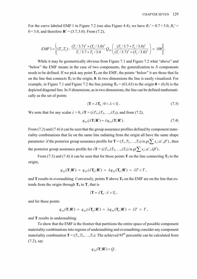
CHAPTER SEVEN 129
For the curve labeled EMF 1 in Figure 7.2 (see also Figure 4.4), we have R1ʹ = 0.7 + 3.0, R2ʹ =
0 + 3.0, and therefore Rʹ = (3.7, 3.0). From (7.2),
2 2 2
1 2 1 21 2 .95 2 2
1 2 1 2
( / 3.7) ( / 3.0) ( / 3.7 / 3.0)1 ( , ) : 100
/ 3.7 / 3.0 ( / 3.7) ( / 3.0)
T T T TEMF T T Q
T T T T
.
While it may be geometrically obvious from Figure 7.1 and Figure 7.2 what “above” and
“below” the EMF means in the case of two components, the generalization to N components
needs to be defined. If we pick any point T0 on the EMF, the points “below” it are those that lie
on the line that connects T0 to the origin, 0. In two dimensions the line is easily visualized. For
example, in Figure 7.1 and Figure 7.2 the line joining T0 = (63, 63) to the origin 0 = (0, 0) is the
depicted diagonal line. In N dimensions, as in two dimensions, the line can be defined mathemati-
cally as the set of points
0{ : 0 1} T T . (7.3)
We note that for any scalar λ > 0, λT = (λT1, λT2, …, λTN), and from (7.2),
.95 .95( ; ) ( ; )q q T R T R . (7.4)
From (7.2) and (7.4) it can be seen that the group assurance profiles defined by component mate-
riality combinations that lie on the same line radiating from the origin all have the same shape
parameter: if the posterior group assurance profile for T = (T1, T2, …, TN) is ( ; , )ig x , then
the posterior group assurance profile for λT = (λT1, λT2, …, λTN) is ( ; , )ig x .
From (7.3) and (7.4) it can be seen that for those points T on the line connecting T0 to the
origin,
.95 .95 0 .95 0( ; ) ( ; ) ( ; )q q q T T T R T R T R ,
and T results in overauditing. Conversely, points T above T0 on the EMF are on the line that ex-
tends from the origin through T0 to T, that is
0{ : 1} T T ,
and for these points
.95 .95 0 .95 0( ; ) ( ; ) ( ; )q q q T T T R T R T R ,
and T results in underauditing.
To show that the EMF is the frontier that partitions the entire space of possible component
materiality combinations into regions of underauditing and overauditing consider any component
materiality combination T = (T1, T2, …, TN). The achieved 95th percentile can be calculated from
(7.2), say
.95 ( ; )q Q T R .

130 OPTIMIZING FOR GROUP CONTEXT, CONSTRAINTS, AND STRUCTURE
Let
T
Q .
From (7.4),
.95 ( ; )q Q T T R
and therefore the component materiality combination λT = (λT1, λT2, …, λTN) lies exactly on the
EMF. If λ > 1 then Q < T and T is in the region of overauditing. If λ < 1 then Q > T and T is in the
region of underauditing.
7.2.2 Constrained component materiality in general
In Section 7.1.1 we saw how to adjust component materiality in a two-component group when it
is constrained for one of the components. In an N-component group component materiality may
be constrained for multiple components, in which case “excess” assurance obtained for the con-
strained components can be offset by relaxing the assurance objectives for the other components
by increasing their component materiality amounts. We do this by computing the component
weight that is implied by each imposed component materiality and then rebalancing the remain-
ing component weights so that weights sum to 1 across the entire group.
If component materiality is constrained to an amount no greater than that otherwise required
for group purposes the first step in rebalancing weights is to determine what component weight is
implied by the constrained component materiality. Suppose for Component i that component ma-
teriality for group audit purposes is Ti and that it is constrained to Ti*, where Ti
* Ti. From (4.18)
the implied component weight wi is the solution to
* .95
.95 .95
1(1/ )
iPi
i
RTRT
Q w R
.
We can write
.95.95 *
.95
(1/ ) 1 iPi i
i
RTRQ w Q
T R
. (7.5)
From (2.10), the solution can be found by applying the Goal Seek tool in Excel to the formula
GammaInv(95%,1/ ,1)i iw Q .
For example, taking the illustration in Section 7.1.1, we have, from (7.1), Q1 = 6.0. Solving
1GammaInv(95%,1/ ,1) 6.0w
gives w1 = 0.36. It is computationally more convenient, however, to have an explicit solution. For

CHAPTER SEVEN 131
this we turn to approximation (2.13), from which
12
2 .95.95
1 1( 1)
12 2 4i i
uw Q u
. (7.6)
For example (noting that u.95 1.645) with Q1 = 6.0 as above,
12
21
1 1.645 16.0 (1.645 1) 0.36
12 2 4w
.
Suppose now that there are multiple components with constrained materiality. We may as-
sume without loss of generality that component materiality is unconstrained for the first k ≥ 1
components and constrained to Ti* Ti for Components k + 1, k + 2, …, N. First we use (7.6) to
compute the implied weights of materiality-constrained components k + 1, k + 2, …, N. The sum
of these implied weights is1
1N
ii kw
.54 If the group consisted only of the k unconstrained
components the weights would be
1
ii k
jj
Yw
Y
for i = 1, 2, …, k and the weights would sum to 1. Because these weights are larger than they
would be were all N of the components unconstrained, we reduce them proportionately for the
implied weights of the constrained components. Therefore, the new weights for the unconstrained
components are
1
1
1Ni
i jk j kjj
Yw w
Y
(7.7)
for i = 1, 2, …, k.
The sum of all N weights is therefore
1 1 11
1
1 1k
N N Nii i iki i k i k
i jj
Yw w w
Y
as required. In summary, component materiality for Components 1, 2, …, N is
.95
.95 .95
*
1 for 1,..., , and(1/ )
for 1,..., .
iP
ii
i
RTRi k
Q w RT
T i k N
(7.8)
where wi is given by equation (7.7).
54 The sum is < 1 because Ti
* Ti.

132 OPTIMIZING FOR GROUP CONTEXT, CONSTRAINTS, AND STRUCTURE
7.3 Leveraging group structure, management style, and scope of controls
To this point we have assumed that groups are comprised of separately managed stand-alone
components so that the group auditor cannot form a conclusion on the group financial statements
by means other than aggregating individual component audit conclusions. In practice, however,
many groups assemble subgroups of components that have similar business activities and these
components share subgroup-level resources and oversight that provide a degree of cohesiveness.
Such a subgroup is referred to here as a cluster.55
Where a cluster exists, the group auditor may be able to treat it as a “virtual single compo-
nent” for group audit planning purposes by forming a prior assurance profile for the cluster as a
whole. Such a cluster prior might be justified by the group auditor’s evaluation of cluster-wide
risks, by tests of the design and operating effectiveness of cluster-wide controls, and/or by the
results of cluster-level analytical procedures. With such a prior, the group auditor can establish a
target cluster posterior by applying equation (4.4) as if for a single component, and then applying
equation (4.9) to determine cluster materiality for the cluster as a whole.
Here it is shown that it is unnecessary to determine separate component materiality amounts
for each component in the cluster. Instead cluster materiality can be used for all the cluster com-
ponents. This essentially provides theoretical support for recognizing the provision in ISA 600
(widely followed in practice) that the group auditor may “identify components at certain levels of
aggregation rather than individually” (see discussion in Section 1.4.2). For the purposes of this
thesis, “cluster” is regarded as synonymous with such an aggregation of components.
7.3.1 Component materiality within clusters
To derive component materiality for cluster members suppose ( ;1, )jLg x is the prior assurance
profile for a cluster of L components as a whole, that is jLX ~ (1, )g . Assuming as before that
the Xj are stochastically independent, ( ;1, )jLg x is the convolution of the prior distributions of
X1, X2, …, XL.56 As will be shown in Section 7.3.3, individual gamma component priors are thus
g(x j; j, ), where the fractional j values equal the component’s relative size, that is,
1
and 1jj jL L
kk
Y
Y
.
55 This term is borrowed from the regulations governing audits of states, local governments and non-profit organ-izations in the United States (OMB 2003). These regulations refer to “a grouping of closely related programs that share common compliance requirements” as a “cluster”. 56 If cluster components operate under commonalities such as cluster-level incentives and performance pressures, the independence assumption may not apply.

CHAPTER SEVEN 133
For a cluster of two equally-sized components,
Component Priors
Cluster Prior1Deconvolute
1 22
( ;0.5, )( ;1, )
( ;0.5, )
g xg x x
g x
.
As to the cluster posterior and likelihood function, if the target posterior is ( ;1, )jLg x , then
target component posteriors are g(x j; j, ʹ) with 1jL . The likelihood distribution required to
update the cluster prior into the cluster posterior is ( ;1, )jLg x B , where B is defined by equation
(2.22). Similarly, an exponential likelihood distribution with parameter B is also required to up-
date the component prior g(x j; j, ) to the component posterior g(x j; j, ʹ). Because cluster and
component materiality are the 95th percentile of the relevant likelihood distribution and because
cluster and component likelihoods are equal, component materiality equals cluster materiality for
each component in the cluster. Figure 7.3 illustrates this.
Figure 7.4, which is somewhat comparable to Figure 4.4 for stand-alone components, illus-
trates the process for a cluster of two equally-sized components. The group auditor establishes an
exponential prior g(x1 + x2; 1, 100 / 0.7) on the cluster and a target cluster posterior
g(x1 + x2; 1, 100 / 3.0), so the cluster likelihood distribution is g(x1 + x2; 1, 100 / 2.3). The cluster
prior deconvolutes into fractional component priors, schematically,
Component Priors
Cluster Prior1Deconvolute
1 22
( ;0.5,100 / 0.7)( ;1,100 / 0.7)
( ;0.5,100 / 0.7)
g xg x x
g x
.
The likelihood distributions are the same at the cluster and component levels so cluster and com-
ponent materialities are the same. Assuming that the audit goes as planned, the component poste-
riors convolute to achieve the desired cluster posterior, schematically,
Component Posteriors
Cluster Posterior1 Convolute
1 22
( ;0.5,100 / 3.0)( ;1,100 / 3.0)
( ;0.5,100 / 3.0)
g xg x x
g x
.
Figure 7.3 Deconvolution and convolution within a cluster.
Deconvolute: components
inherit fractions of cluster prior
Convolute:components aggregate to form cluster
posterior
1
1/ 1/ B
1 2
Cluster prior
( ;1, )g x x
1 1
2 2
1 2
Component priors
( ; , )
( ; , )
1
g x
g x
1 1
2 2
1 2
Component posteriors
( ; , )
( ; , )
1
g x
g x
1 2
Cluster posterior
( ;1, )g x x 1 2
Cluster likelihood
( ;1, )g x x B
1
2
Component likelihoods
( ;1, )
( ;1, )
g x B
g x B

134 OPTIMIZING FOR GROUP CONTEXT, CONSTRAINTS, AND STRUCTURE
Cluster Components 1 & 2 Cluster
Priors = g(xj; 0.5, 100 / 0.7) Prior = g(x1 + x2; 1, 100 / 0.7)
Likelihoods = g(xj; 1, 100 / 2.3) Posteriors = g(xj; 0.5, 100 / 3.0)
Likelihood = g(x1 + x2; 1, 100 / 2.3)Posterior = g(x1 + x2; 1, 100 / 3.0)
Figure 7.4 Example of cluster with two identical components.
7.3.2 Illustration of the effects of cluster-level prior assurance
We close with an extended example that illustrates the dramatic reduction of component audit
cost possible when the group auditor can form prior cluster-level assurance.
Figure 7.5, Figure 7.6, and Figure 7.7 present various scenarios for a group comprised of
ten equally-sized units across three business groupings: six Retail components, three Manufactur-
ing components, and one Real Estate component.
In Figure 7.5, the components are all stand-alone and there is negligible prior assurance for
each component. Each component materiality is Ti = 19 (see the N = 10 row in Table 5.2) and
RTVC = 5.24 with the Retail components comprising 3.14 of the total.
In Figure 7.6, the group auditor has evaluated group-level controls for each Retail compo-
nent individually and determined that there is moderate (RMM1j = 50%) prior assurance for each.
Component materiality for each Retail component is 23 (= 19 × 1.231 per Table 4.2), which re-
duces RTVC across the six Retail components to 2.55, while the other four components remain
the same and group RTVC drops to 4.65.
In Figure 7.7, the group auditor is able to form a cluster prior for the Retail components.
We thus have one virtual component of size 6 (comprising the six Retail components) and four
components of size 1. The auditor assesses a moderate profile (RMM1 = 50%) for the Retail clus-
ter. Cluster materiality is 64 and, because there is a basis for treating the six units as a virtual sin-
gle component, each of the six Retail components is audited using T1j = 64 and RTVC drops to
0
.04
0 50 100 150
g(x1)
x1
0
.04
0 50 100 150
g(x2)
x2
0
.04
0 50 100 150
g(x)
x = x1 + x2
0
.04
0 50 100 150
g(x1)
x1
0
.04
0 50 100 150
g(x2)
x2
0
.04
0 50 100 150
g(x)
x = x1 + x2

CHAPTER SEVEN 135
0.94 or 33% of Retail units in Figure 7.5.57 Also, even though nothing has changed for the three
Manufacturing and one Real Estate units, component materialities are now 27 and RTVC drops
from 1.57 to 1.11, and from 0.52 to 0.37, respectively. For the group as a whole, the presence of
the Retail cluster and its moderate prior allows a reduction in aggregate RTVC of more than 50%
with reductions in every component while maintaining the AGA at 95%. This significant change
occurs because the group in Figure 7.7 effectively consists of five stand-alone components: one
large virtual single component (the cluster) plus four individual standalone components compared
with the ten stand-alone components in Figure 7.5 and Figure 7.6.
This illustration shows the sizeable reduction in component audit cost that is possible from
the group auditor’s reliance on cluster-level prior assurance. The example does not address the
development of reliable prior assurance for a cluster as a whole, which is likely to be costly. Such
a prior would require the existence, identification, and analysis of a group’s business activities
that have substantial cohesiveness, exploitable similarities, and common controls as well as tests
of the design and operating effectiveness of cluster-level controls. However, the potential for
component audit cost savings via clusters highlights the importance of conceptual models, ar-
chival analyses of extant audit practices, and behavioral studies to support reliable auditing pro-
cedures for assessing cluster and other group-level controls and risks.
Figure 7.5 Group with ten equally-sized components in three industry segments, negligible priors.
57 Cluster weight is 1
60.38
6 4 1w
, and per equation (4.18), 1
.95
100 3.0 0.71 64
(1/ 0.38) 3.0T
Q
.
T = 100
T11 = 19
T13 = 19
T12 = 19
T21 = 19
T23 = 19
T22 = 19
1. Retailnegligible priors
2. Manufacturingnegligible priors
3. Real Estatenegligible priors
T14 = 19
T16 = 19
T15 = 19
T3 = 19
RTVC1 = 3.14(60%)
RTVC2 = 1.57(30%)
RTVC3 = 0.52(10%)
RTVC = 5.24(100%)

136 OPTIMIZING FOR GROUP CONTEXT, CONSTRAINTS, AND STRUCTURE
Figure 7.6 As Figure 7.5 but with group-level controls for each Retail component individually.
Figure 7.7 As Figure 7.5 but with a Retail cluster prior.
T = 100
T11 = 23
T13 = 23
T12 = 23
T21 = 19
T23 = 19
T22 = 19
1. Retailcomponent priors
2. Manufacturingnegligible priors
3. Real Estatenegligible priors
T14 = 23
T16 = 23
T15 = 23
T3 = 19
RTVC1 = 2.55(55%)
RTVC2 = 1.57(34%)
RTVC3 = 0.52(11%)
RTVC = 4.65(100%)
T = 100
T1 = 64
T11 = 64
T13 = 64
T12 = 64
1. Retailcluster prior
2. Manufacturingnegligible priors
3. Real Estatenegligible priors
T14 = 64
T16 = 64
T15 = 64
T21 = 27
T23 = 27
T22 = 27
T3 = 27
RTVC1 = 0.94(39%)
RTVC2 = 1.11(46%)
RTVC3 = 0.37(15%)
RTVC = 2.42(100%)
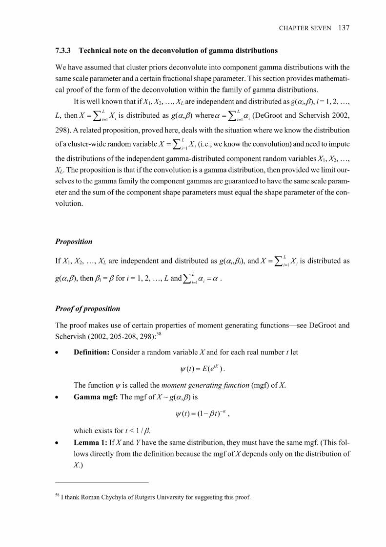
CHAPTER SEVEN 137
7.3.3 Technical note on the deconvolution of gamma distributions
We have assumed that cluster priors deconvolute into component gamma distributions with the
same scale parameter and a certain fractional shape parameter. This section provides mathemati-
cal proof of the form of the deconvolution within the family of gamma distributions.
It is well known that if X1, X2, …, XL are independent and distributed as g(i, ), i = 1, 2, …,
L, then1
L
iiX X
is distributed as g(, ) where
1
L
ii
(DeGroot and Schervish 2002,
298). A related proposition, proved here, deals with the situation where we know the distribution
of a cluster-wide random variable1
L
iiX X
(i.e., we know the convolution) and need to impute
the distributions of the independent gamma-distributed component random variables X1, X2, …,
XL. The proposition is that if the convolution is a gamma distribution, then provided we limit our-
selves to the gamma family the component gammas are guaranteed to have the same scale param-
eter and the sum of the component shape parameters must equal the shape parameter of the con-
volution.
Proposition
If X1, X2, …, XL are independent and distributed as g(i, i), and1
L
iiX X
is distributed as
g(, ), then i = for i = 1, 2, …, L and1
L
ii
.
Proof of proposition
The proof makes use of certain properties of moment generating functions—see DeGroot and
Schervish (2002, 205-208, 298):58
Definition: Consider a random variable X and for each real number t let
( ) ( )tXt E e .
The function ψ is called the moment generating function (mgf) of X.
Gamma mgf: The mgf of X ~ g(, ) is
( ) (1 )t t ,
which exists for t < 1 / .
Lemma 1: If X and Y have the same distribution, they must have the same mgf. (This fol-
lows directly from the definition because the mgf of X depends only on the distribution of
X.)
58 I thank Roman Chychyla of Rutgers University for suggesting this proof.
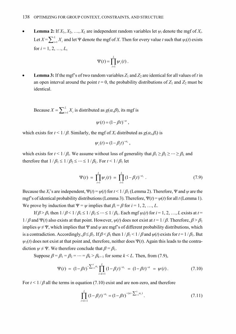
138 OPTIMIZING FOR GROUP CONTEXT, CONSTRAINTS, AND STRUCTURE
Lemma 2: If X1, X2, …, XL are independent random variables let ψi denote the mgf of Xi.
Let X =1
L
iiX
and let Ψ denote the mgf of X. Then for every value t such that ψi(t) exists
for i = 1, 2, …, L,
1
( ) ( )L
ii
t t
.
Lemma 3: If the mgf’s of two random variables Z1 and Z2 are identical for all values of t in
an open interval around the point t = 0, the probability distributions of Z1 and Z2 must be
identical.
Because
1
L
iiX X
is distributed as g(, ), its mgf is
( ) (1 )t t ,
which exists for t < 1 / . Similarly, the mgf of Xi distributed as g(i, i) is
( ) (1 ) ii it t ,
which exists for t < 1 / i. We assume without loss of generality that 1 ≥ 2 ≥ ⋯≥ L and
therefore that 1 / 1 1 / 2 ⋯ 1 / L. For t < 1 / 1 let
1 1
( ) ( ) (1 ) i
L L
i ii i
t t t
. (7.9)
Because the Xi’s are independent, Ψ(t) = ψ(t) for t < 1 / 1 (Lemma 2). Therefore, Ψ and ψ are the
mgf’s of identical probability distributions (Lemma 3). Therefore, Ψ(t) = ψ(t) for all t (Lemma 1).
We prove by induction that Ψ = ψ implies that i = for i = 1, 2, …, L.
If > 1 then 1 / < 1 / 1 1 / 2 ⋯ 1 / L. Each mgf ψi(t) for i = 1, 2, …, L exists at t =
1 / and Ψ(t) also exists at that point. However, ψ(t) does not exist at t = 1 / . Therefore, > 1
implies ψ ≠ Ψ, which implies that Ψ and ψ are mgf’s of different probability distributions, which
is a contradiction. Accordingly, 1. If < 1 then 1 / 1 < 1 / and ψ(t) exists for t = 1 / 1. But
ψ1(t) does not exist at that point and, therefore, neither does Ψ(t). Again this leads to the contra-
diction ψ ≠ Ψ. We therefore conclude that = 1.
Suppose = 1 = 2 = ⋯= k > k + 1 for some k < L. Then, from (7.9),
1
1
( ) (1 ) (1 ) (1 ) ( )k
ii i
L
ii k
t t t t t
. (7.10)
For t < 1 / all the terms in equation (7.10) exist and are non-zero, and therefore
1( )
1
(1 ) (1 )k
ii i
L
ii k
t t
. (7.11)

CHAPTER SEVEN 139
We note that1
k
ii
is positive and therefore
1( )*( ) (1 )
kiit t
is the mgf of X distributed as1
( , )k
iig
.59 Similarly, we may write the left-hand side of
(7.11) as
*
1
( ) (1 ) i
L
ii k
t t
,
which is the mgf of1
L
ii kX
. Because Ψ*(t) = ψ*(t) in the open interval t < 1 / , it follows that
1
L
ii kX
is also distributed as1
( , )k
iig
(Lemma 3). We can now reprise the previous ar-
gument with ψ*(t) in place of ψ(t) and Ψ*(t) in place of Ψ(t). Because > k+1 therefore 1 / <
1 / k+1, which means that Ψ*(t) exists at t = 1 / but ψ*(t) does not, and therefore Ψ* ≠ ψ*, which
is a contradiction. Therefore, = k+1 and, by induction, i = for i = 1, 2, …, L. Finally, because
1( ) (1 )L
iit t
and
( ) (1 )t t ,
it follows that Ψ = ψ implies
1
L
ii
.
Fractional shape value
As regards the value of i, we note that it is reasonable to assume that Var(Xi) is proportional to
Yi, the size of Component i. From (2.5), Var(Xi) = i 2, from which it follows that i Var(Xi)
Yi and
ii
j
Y
Y
.
59 From (7.11), given that > k+1, 1 1 1
( ) log(1 ) log(1 ) log(1 )k L L
i i i ii i k i kt t t
. There-
fore,1 1
0k L
i ii i k
.

140 OPTIMIZING FOR GROUP CONTEXT, CONSTRAINTS, AND STRUCTURE
7.4 Significant opportunities for optimization
This chapter has presented two approaches to optimizing component materiality. The first makes
use of the fact that there is a continuum of component materiality combinations that result in the
group auditor’s assurance objective being achieved. That continuum is the efficient materiality
frontier, and determining which component materiality is optimal for given circumstances
amounts to computing the optimal point on EMF—typically the combination that minimizes cost
for the group as a whole.
The second approach to optimization is to leverage the clustering of components that is typ-
ical for groups found in practice. This essentially allows the group auditor to determine compo-
nent materiality at a level of aggregation rather than at the individual component level. This ap-
proach, which is followed in practice and recognized in ISA 600, can lead to significant efficien-
cy improvements. This chapter has provided a framework for the approach and shown how effi-
ciency gains can be measured.
It is important to keep in mind that the GUAM method produces an algorithmically optimal
solution based on an abstract model. To the extent that reality deviates from the model or there
are conditions external to the model, the GUAM solution may not be the best and further adjust-
ment may be necessary based on professional judgment. For example, the GUAM method adjusts
component materiality throughout the group to respond to constraints over one or more compo-
nent materiality amounts. This may not be an optimal strategy if, for example, it increases litiga-
tion risk, in which case the group auditor may choose to override GUAM.
141
CHAPTER 8 Software Implementation
This chapter describes software I have developed to implement the GUAM component materiali-
ty method. A detailed algorithm is presented in pseudocode to facilitate porting to any software
platform. Besides providing a practical solution to a specific problem, the software illustrates a
wider point, which is that quite complex, computationally-demanding Bayesian methods can be
implemented in forms that are easy for any auditor to access and use. This is a far cry from the
days not so long ago when scholars and practitioners could describe the possibilities of Bayesian
modeling with continuous probability distributions but lacked the tools to realize them—see
Leslie (1984) and Kinney (1984) quoted in Section 2.2. The software is available to scholars,
practitioners, and others in the hope is that this will encourage them to explore, apply, and extend
the GUAM model and method.
8.1 General description
The software described here, named “GUAMcalc”, is an Excel 2007 workbook that implements
the GUAM component materiality method. It contains four worksheets as can be seen from the
tabs depicted in Figure 8.1:
Calculator. This is the main worksheet, depicted in Figure 8.1.
Help. This provides a basic level of help for users who are generally familiar with the
GUAM method.
Policy Settings. Certain audit parameters that are usually a matter of firm policy are set
here.
About, Copyright (c). This describes the workbook in general terms and carries a copy-
right notice, usage terms (which are permissive), and a warranty disclaimer.
For ease of implementation and modification, the workbook is in plain vanilla Excel with
no macros or special functions. To reduce inadvertent user errors, worksheets are protected so
that only input cells may be selected, input data are validated using the Excel Data Validation fea-
ture, and the main algorithm in Calculator is performed in hidden columns. The workbook struc-
ture is protected, which means that worksheets cannot be added or deleted. Password protection is

142 SOFTWARE IMPLEMENTATION
Figure 8.1 The GUAMcalc workbook.
not used so that the workbook and individual worksheets can be unprotected if necessary. Firms
implementing GUAMcalc would probably modify the workbook to reflect firm policies and pref-
erences and to strengthen the level of protection.
8.2 Policy settings worksheet
Audit parameters that are usually a matter of firm policy are set in the Policy Settings tab depict-
ed in Figure 8.2. The workbook comes with “factory” settings that are also displayed on the
screen so that the user can revert to them if necessary.
Desired Group Assurance. This is the group auditor’s judgment as to what constitutes rea-
sonable assurance, the complement of an acceptably low level of risk. The factory setting is 95%.
This may be changed via a drop-down box that offers the choices shown in Table 8.1. The associ-
ated R factors per equation (2.16) are also tabulated.

CHAPTER EIGHT 143
Table 8.1 Levels of assurance available in GUAMcalc
Desired Group Assurance
R Factor
90% 2.30 95% 3.00 98% 3.91 99% 4.61
Prior Assurance Table. This table lists the levels of prior component assurance that the
group auditor can choose from in the Calculator worksheet. The table provides six descriptive
levels. The descriptions are mapped to quantified probabilities. The default setting is the same as
Table 2.2. R factors are also displayed in the table. The last column in the table shows the in-
crease in component materiality that results from the specified prior assurance.
Figure 8.2 The Policy Settings tab.
8.3 Calculator worksheet
The Calculator worksheet is depicted in Figure 8.3. Input fields have a white background and cal-
culated fields have a lightly shaded background. The Calculator worksheet is pre-configured to
Desired Group Assurance 95% R‐Factor 3.00
"Factory" Setting 95% 3.00
PRIOR ASSURANCE TABLE
Description Probabil ity R Probabil ity RComponent
Materiality Increase
Negligible 0% 0.0 0.0% 0.0 0.0%
Very Low 10% 0.1 9.7% 0.1 3.5%
Low 30% 0.4 27.3% 0.3 11.9%
Moderate 50% 0.7 43.0% 0.6 23.1%
High 70% 1.2 57.6% 0.9 40.2%
Very High 90% 2.3 72.8% 1.3 76.9%
"Factory" Settings*
Negligible 0% 0.0 0.0% 0.0 0.0%
Very Low 10% 0.1 9.7% 0.1 3.5%
Low 30% 0.4 27.3% 0.3 11.9%
Moderate 50% 0.7 43.0% 0.6 23.1%
High 70% 1.2 57.6% 0.9 40.2%
Very High 90% 2.3 72.8% 1.3 76.9%
* Probability Percentages Based on SAS 39, Table 2
Relative to Final
Component Materiality
Relative to Initial
Component Materiality

144 SOFTWARE IMPLEMENTATION
Figure 8.3 The Calculator worksheet.
handle up to 20 components and more can be added if necessary. Table 8.2 lists the input data
fields. Most fields have default values and can be left blank. Table 8.3 lists the computed fields.
Labels “a” through “m” identify the fields as depicted in Figure 8.3.
Table 8.2 Data input fields
Label Field Valid Data Explanation
a Group Materi-ality, T
Whole number > 0, or blank
Group auditor’s professional judgment about materiality for the group financial statements as a whole: $100,000 in Figure 8.3. If the field is blank (or 100), Component Materiality is displayed as a percentage of Group Materiality.
b Desired Group Assurance, C
Percentage The audit firm’s policy about what constitutes reasonable assur-ance: 95% in Figure 8.3. This is a policy setting and can only be changed in the Policy Settings tab.
c Component Name
Any name, or none
The name or description of the component: Component 1, …, Component 3 in Figure 8.3. If the name it is too long it will not display correctly in the chart (Figure 8.4).
d Component Size, Yi
Whole number > 0
Typically Revenues, Total Assets, or some other financial bench-mark. For example, in Figure 8.3, Y1 = $9,000,000. Only relative size matters, so the amounts need not be in the same units as Group Materiality.
f Variable Cost per Unit, VCUi
Blank or dec-imal number
The relative variable cost per unit to audit. For example, in Figure 8.3, VCU3 = 0.6, while, implicitly, because the fields have been left blank, VCU1 = VCU2 = 1.
g Prior Compo-nent Assurance
From drop-down list, or blank
The group auditor’s prior component assurance. For example, in Figure 8.3, it is moderate for Component 1 and high for Compo-nent 2. For Component 3 it is negligible, effectively zero, as signi-fied by a blank field.
h Constrained Component Materiality, Ti
*
Whole number > 0 (zero or blank = uncon-strained)
The amount, if any, to which Component Materiality is con-strained, expressed in the same units as Group Materiality. For example, in Figure 8.3, Component 2 materiality is limited to T2
* = $35,000, while it is unconstrained for Components 1 and 3. If the specified constrained value exceeds Component Materiality required for group audit purposes the tick mark “>” is displayed and the constraint is ignored.
a Group Materiality 100,000 k Achieved Group 95‐th Percentile 100,272 b Desired Group Assurance 95% l Achieved Group Assurance (AGA) 94.94%
m Relative Total Variable Cost (RTVC) 1.76
Component Name
Variable
Cost per
Unit
Group
Auditor's
Prior
Assurance
c d e f g h i j
Total 15,000,000 1.00 35,000 160,712 1.00
1 Component 1 9,000,000 0.60 Moderate 95,954 0.60
2 Component 2 5,000,000 0.33 High 35,000 35,000 0.22
3 Component 3 1,000,000 0.07 0.60 29,757 0.19
4 ‐ ‐ ‐
5 ‐ ‐ ‐
Component Size
Constrained
Component
Materiality
Component Materiality

CHAPTER EIGHT 145
Table 8.3 Computed fields
Label Field Explanation
e Relative Component Size i
j
Y
Y. For example, in Figure 8.3, the relative size of Component 1 is
9,000,000 / 15,000,000 = 0.60.
i Component Materiality, Ti As computed per the GUAM method
j Relative Component Ma-teriality
i
j
T
T. For example, in Figure 8.3, the relative size of T1 is
95,954 / 160,712 = 0.60.
k Achieved Group Percen-tile
This is the 100 C-th percentile of the group assurance profile. It should approximately equal T, the specified Group Materiality [a], the differ-ence being the result of certain mathematical approximations in the GUAM algorithm. For example, in Figure 8.3, the Achieved Group 95th Percentile is $100,272 compared with Group Materiality of $100,000—an “error” of less than 3 / 1000. See Sections 4.4 and 6.2.
l Achieved Group Assur-ance (AGA)
This is the actual group assurance that total group misstatement does not exceed Group Materiality based on the group assurance profile. It should approximately equal C, the specified Desired Group Assurance [b], the difference being the result of certain mathematical approximations in the GUAM algorithm. For example, in Figure 8.3, AGA = 94.94% compared with C = 95%. See Sections 5.3 and 6.2.
m Relative Total Variable Cost (RTVC)
This is the ratio of Total Variable Cost using indicated Component Materialities and using Group Materiality throughout. For example, in Figure 8.3, RTVC = 1.76. See Section 5.2.
Relative Component Size and Relative Component Materiality are charted in descending
order of Component Size as depicted in Figure 8.4. The chart is designed to help users visualize
the shape of the group and the relationship between component materiality and size.
Figure 8.4 Relative component materiality compared with relative component size.
.0
.1
.2
.3
.4
.5
.6
.7
Component 1
Component 2
Component 3
Relative Component Size and Materiality in Descending Order of SizeSize
Materiality

146 SOFTWARE IMPLEMENTATION
8.4 GUAM algorithm
The mathematical basis for the GUAM algorithm is set forth in Chapter 4 through Chapter 7.
Here we focus on programming it. The algorithm is presented in a simple pseudocode loosely
based on Excel Visual Basic for Applications (VBA). This simplifies the task of re-implementing
the algorithm in other software.
8.4.1 Notation
Table 8.4 shows the overall application parameters and constants and Table 8.5 shows the com-
ponent-level variables used in the GUAM algorithm as implemented in the Calculator worksheet.
The “Steps” identified in the last columns refer forward to Table 8.6. Elsewhere in this thesis the
parameters of prior assurance profiles are designated and , while those of posterior assurance
profiles are designated ʹ and ʹ. Because in the actual GUAM algorithm documented here it is
not necessary to directly use the prior parameters, the notation is simplified by eliminating the
primes and designating the posterior parameters and .
Table 8.4 Group-level/global variables and constant initialization
Notation Description First Use
, Shape and scale parameters of the group assurance profile Step 22, 23
AGA Achieved Group Assurance Step 25
C Desired Group Assurance [b] and desired component assurance. The “factory setting” is C = 95% but it can be changed in Policy Settings.
Input
MAX = 20 Maximum number of components. Initialization
MAX_ALPHA = 380 Maximum value of for which GammaInv is reliable—based on tests performed with Excel 2003 (Excel 2007 can correctly handle somewhat larger values)
Initialization
RC = −ln(1−C) R factor corresponding to C; R.95 = 2.9957… (approx 3.0) Initialization
RTVC Relative Total Variable Cost Step 26
T Group Materiality [a]; default value is T = 100 Input
uc Standard normal 100 C-th percentile; u.95 = 1.6448… Initialization
Table 8.5 Component variables
Notation Description First Use
i, i* Scale parameter of assurance profile Step 6, 12
Descriptioni Description of group auditor’s prior assurance Input
Pi Prior probability Step 8
iPR R factor for probability Pi,iPR = −ln(1 − Pi) Step 9
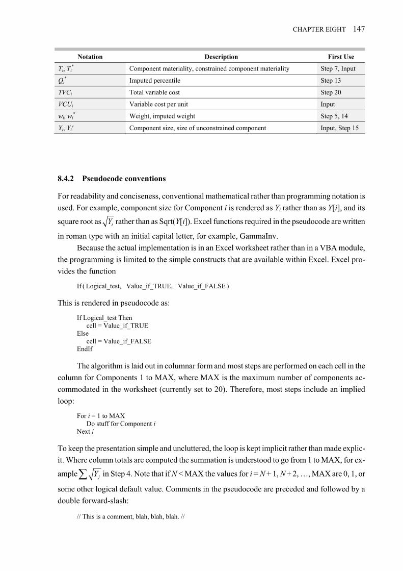
CHAPTER EIGHT 147
Notation Description First Use
Ti, Ti* Component materiality, constrained component materiality Step 7, Input
Qi* Imputed percentile Step 13
TVCi Total variable cost Step 20
VCUi Variable cost per unit Input
wi, wi* Weight, imputed weight Step 5, 14
Yi, Yiʹ Component size, size of unconstrained component Input, Step 15
8.4.2 Pseudocode conventions
For readability and conciseness, conventional mathematical rather than programming notation is
used. For example, component size for Component i is rendered as Yi rather than as Y[i], and its
square root as iY rather than as Sqrt(Y[i]). Excel functions required in the pseudocode are written
in roman type with an initial capital letter, for example, GammaInv.
Because the actual implementation is in an Excel worksheet rather than in a VBA module,
the programming is limited to the simple constructs that are available within Excel. Excel pro-
vides the function
If ( Logical_test, Value_if_TRUE, Value_if_FALSE )
This is rendered in pseudocode as:
If Logical_test Then cell = Value_if_TRUE Else cell = Value_if_FALSE EndIf
The algorithm is laid out in columnar form and most steps are performed on each cell in the
column for Components 1 to MAX, where MAX is the maximum number of components ac-
commodated in the worksheet (currently set to 20). Therefore, most steps include an implied
loop:
For i = 1 to MAX Do stuff for Component i Next i
To keep the presentation simple and uncluttered, the loop is kept implicit rather than made explic-
it. Where column totals are computed the summation is understood to go from 1 to MAX, for ex-
ample jY in Step 4. Note that if N < MAX the values for i = N + 1, N + 2, …, MAX are 0, 1, or
some other logical default value. Comments in the pseudocode are preceded and followed by a
double forward-slash:
// This is a comment, blah, blah, blah. //

148 SOFTWARE IMPLEMENTATION
8.4.3 The GUAMcalc component materiality algorithm step by step
The GUAMcalc component materiality algorithm is explained step by step in Table 8.6. Each
step corresponds to a column in the Calculator worksheet. The following section contains a
worked example.
Table 8.6 GUAM component materiality algorithm step by step
Step Description Method Ref
0 Initialization
C = Desired Group Assurance [b] RC = −ln(1−C) T = Group Materiality [a] uC = NormsInv(C) // Standard normal percentile // Prior Assurance table // From Policy Settings worksheet //
1 Get component size from Input
Yi = ComponentSize [d]
2 Get variable cost per unit from Input
If VCUi [f] > 0 Then VCUi = VCUi [f] Else VCUi = 1 EndIf
3 Calculate cost-adjusted component size
Yi = VCUi × Yi
Initial calculation of component materiality
4 Square roots for weighting
Compute iY
Compute jY
5 Component weights
If 0jY Then
ii
j
Yw
Y
Else wi = 0 EndIf
(4.6)

CHAPTER EIGHT 149
Step Description Method Ref
6 Component scale pa-rameter
If wi > 0 Then If 1 / wi MAX_ALPHA Then GammaInv( ,1/ ,1)i iT C w
Else
22 11 4
14 12
Ci C
i
uT u
w
EndIf Else 0i
EndIf
(4.4) (2.11)
7 Component materiali-ty (initial) i C iT R (4.10)
Inflating component materiality for group auditor’s prior component assurance
8 Prior probability
// Use description of Group Auditor’s Prior Assurance [g] to look up corresponding Probability in the Prior Assurance Table and Set Pi = Probability. // If Descriptioni does not match a table entry (i.e., it’s blank) Then Pi = 0 Else Pi = Probabilityi corresponding to matching Descriptioni EndIf
9 Prior R factor ln(1 )iP iR P (2.16)
10 Prior-adjusted com-ponent materiality
1 iP
i iC
RT T
R
(4.17)
Adjusting component materiality for constrained component materiality
11 Constrained compo-nent materiality
If ConstrainedComponentMateriality [h] Ti Then *
iT ConstrainedComponentMateriality [h]
Else * 0iT
EndIf
12 Imputed scale param-eter for constrained component
// By analogy with Steps 7-10, materiality (constrained) after ad-justing for the prior is * * (1 / )
ii C i P CT R R R . Therefore, // *
*
(1 / )i
ii
C P C
T
R R R

150 SOFTWARE IMPLEMENTATION
Step Description Method Ref
13 Imputed percentile for constrained compo-nent
If * 0i Then
**ii
TQ
Else * 0iQ
EndIf
(4.4)
14 Imputed weight of constrained compo-nent
If * 2( 1) /12i CQ u Then
22
* * 1 11
12 2 4C C
i i
u uw Q
Else * 0iw
EndIf
(7.6) (2.13)
Compute *jw
15 Eliminate constrained components
If * 0iw Then
0iY
Else i iY Y
EndIf
16 Recompute square roots for remaining components
Compute iY
Compute jY
17 Recompute weights, adjusting for con-strained components
If * 0iw Or 0jY
*i iw w
Else
*1 ii j
j
Yw w
Y
EndIf // Note that 1iw as required //
(7.7)

CHAPTER EIGHT 151
Step Description Method Ref
18 Revised component scale parameters
If * 0i Then
*i i
Else If wi > 0 Then If 1 / wi MAX_ALPHA Then GammaInv( ,1/ ,1)i iT C w
Else
22 11 4
14 12
Ci C
i
uT u
w
EndIf Else 0i
EndIf EndIf
(4.4) (2.11)
19
Recompute compo-nent materiality or set equal to constrained value
If * 0iT Then
*i iT T
Else
1 iP
i i CC
RT R
R
EndIf
(7.8)
Cost calculation
20 Total variable cost
If Ti > 0 Then
/
ii
i C
YTVC
T R
Else 0iTVC
EndIf
(5.1)
Compute iTVC
Final summary calculations for group assurance profile
21 Mean and variance i iE X ,
2Var i iX
(2.23) (2.24)

152 SOFTWARE IMPLEMENTATION
Step Description Method Ref
22 parameter
If Var 0iX Then
2
Var
i
i
E X
X
Else = 0 EndIf
(2.25)
23 parameter
If 0iE X Then
Var i
i
X
E X
Else = 0 EndIf
(2.26)
24 100 Cth percentile
If > 0 GammaInv( , ,1)Percentile C
Else Percentile = 0 EndIf
(2.10)
25 Achieved group as-surance (AGA)
If > 0 and > 0 Then ( , , ) GammaDist( / , ,1,TRUE)AGA G T T
Else AGA = 0 EndIf
(5.5)
26 Relative total variable cost (RTVC)
Denominator =/
i
C
Y
T R // Recall Yi = VCUi × Yi in Step 3 //
If Denominator > 0
iTVCRTVC
Denominator // Numerator from Step 20 //
Else RTVC = 0 EndIf
(5.3)
8.4.4 Worked step-by-step example of the algorithm
A worked numerical example of the algorithm detailed in Table 8.6 is shown in Table 8.7. It uses
the example depicted in Figure 8.3. While the orientation of this table is by row, the steps in the
actual worksheet are arranged by column.

CHAPTER EIGHT 153
Table 8.7 Calculation example
Step Description Component 1 Component 2 Component 3 Total
Initialization
0 C = Group assurance 95% - RC=−ln(1−C) 2.996 - T = Group materiality 100,000 - uc = NormsInv(C) 1.645
Input data
1 Yi 9,000,000 5,000,000 1,000,000 15,000,000 2 VCUi 1 1 0.6 3 Yi = VCUi × Yi 9,000,000 5,000,000 600,000 14,600,000 4 √Yi 3,000 2,236 775 6,011
Initial calculation
5 Initial wi 0.4991 0.3720 0.1289 1.0000 6 Initial βi 21,054 17,169 7,790 7 Initial Ti 63,073 51,434 23,338 137,845
Inflation for prior
8 Prior Pi 50% 70%
9 Prior R factoriPR 0.69 1.20
10 Prior-Adjusted Ti 77,667 72,106 23,338 173,110
Adjustment for constrained Ti
11 Constrained Ti* 35,000 35,000
12 Imputed βi* 8,334
13 Imputed Percentile Q* 12.00 14 Imputed wi
* 0.1405 0.1405 15 Remaining Yiʹ 9,000,000 600,000 9,600,000 16 √Yiʹ 3,000 775 3,775 17 wi 0.6832 0.1405 0.1764 1.0000 18 βi 26,012 8,334 9,933 44,279 19 Ti 95,954 35,000 29,757 160,712
Cost calculation
20 TVCi 280.98 427.96 60.40 769.35
Summary
21 E(X) = ∑βi 44,279 - Var(X) = ∑βi
2 844,733,111 22 2.32 23 19,078 24 Achieved percentile 100,272 25 AGA 94.94% 26 Den = (∑Yi) / (T / RC) 437.38 - Num = ∑TVCi 769.35 - RTVC = Num / Den 1.76


155
CHAPTER 9 Conclusions
This chapter concludes my thesis by summarizing its contributions to auditing and suggesting op-
portunities for further research and development.
9.1 Contributions to auditing
This thesis makes three contributions to auditing theory and practice:
A Bayesian generalization and extension of the profession’s standard audit risk model
A theoretically-grounded solution to the component materiality problem
An algorithm and specific software implementation for determining component materiality
These contributions are potentially of interest to various constituents including auditing standards
setters, partners in accounting firms responsible for determining audit policies and methodolo-
gies, individual practitioners, regulators and practice inspectors, scholars engaged in audit re-
search, and others concerned with effective and efficient group audits.
9.1.1 Generalization and extension of the audit risk model
The GUAM model is a Bayesian generalization and extension of the profession’s widely-used
standard audit risk model. It utilizes the gamma family of probability distributions. GUAM is a
true generalization in the strong sense that it delivers the same probabilities as ARM in simple
situations where ARM works correctly, but it also correctly models assurance in more complex
situations where ARM fails. The key generalization is representing assurance by probability dis-
tributions not just point probabilities. This generalization makes it possible to aggregate assurance
across components—a significant extension that makes GUAM suitable for modeling group au-
dits, which by definition involve multiple components. There is no construct for aggregation in
ARM, which is strictly a single-entity model.
9.1.2 The GUAM method for determining component materiality
The GUAM model is applied to solve a longstanding problem in auditing—the determination of
optimal component materiality combinations that in totality achieve the group assurance objective
within the framework of the ISAs.

156 CONCLUSIONS
The GUAM method determines component materiality combinations that are designed to
achieve the group auditor’s assurance objective while minimizing total audit cost. The method
incorporates the group auditor’s prior assurance on components, accommodating various configu-
rations of group-level controls and group structures. The GUAM method leads to an efficient ma-
teriality frontier—a continuum of materiality combinations that achieve the group assurance ob-
jective. Component sizes and other constraints are used to locate the optimal component material-
ity combination on the EMF (usually the combination that minimizes cost). The result is a model
for group audit assurance under stylized conditions and a conceptual basis for devising extensions
and solutions to deal with deviations from the stylized ideal. As with any model, there are often
facts and circumstances beyond its scope that must be taken into account. The model facilitates
but does not replace professional judgment.
Alternative methods to determine component materiality allowed by ISA 600 and used in
contemporary group audit practice result in component materiality combinations that vary widely
and imply substantially different levels of audit effort and, depending on circumstances, may be
ineffective in meeting professional standards, inefficient in the use of resources, or both ineffec-
tive and inefficient. This disparity suggests the need for more definitive authoritative guidance,
for which the GUAM method is a possible basis.
9.1.3 Practical implementation of the GUAM method
The GUAM method requires software support for it to be implemented in the field. Because of its
ubiquity and familiarity, Microsoft Excel is an appealing platform. This thesis describes a specific
implementation of the GUAM method in Excel including a detailed component materiality algo-
rithm. The algorithm is presented in pseudocode for portability.
Besides providing a specific solution to a specific problem, the software demonstrates that
the GUAM model is not just an analytical framework but can also lead to practical solutions ac-
cessible to any auditor. This is a far cry from the days not so long ago when scholars and practi-
tioners could describe the possibilities of Bayesian modeling but lacked the necessary tools.
The software itself is available to scholars, practitioners, and others in order to encourage
exploration, application, and extension of the GUAM model and method.
9.2 Opportunities for further research and development
The GUAM audit assurance model has the potential to contribute to the understanding and solu-
tion of other assurance-related problems in auditing where progress has been stymied for want of
a suitable analytical or computational framework; and this thesis highlights other potential ave-
nues for research.

CHAPTER NINE 157
9.2.1 Group audit practice and theory
Little is known about the effectiveness and efficiency of current group audit practices. Further-
more, since ISA 600 only went into effect starting with 2010 audits, practices, including the de-
termination of component materiality, have not settled and are still evolving. There is a need for
comparative archival and behavioral research to support best practices, and to facilitate standards
setting and the development of authoritative guidance for planning group audits under practical
conditions.
Group-wide controls is a new construct in ISA 600 and the model employed in this thesis
for how they affect the group auditor’s prior assurance is relatively simple. Little is known about
their design and operating effectiveness, suggesting a need for theoretical and behavioral re-
search. Further, this thesis simply assumes specific values for group-level component and cluster
priors. In practice, group auditors must form and be able to defend their particular priors for com-
ponents and clusters. Research is needed regarding the conceptual underpinnings, design, and op-
erating effectiveness of group-level controls and their impact on priors.
The GUAM method as presented in this thesis assumes that all N components are audited
using component materiality. This is a simplification that applies only if every component is indi-
vidually financially significant to the group financial statements. Real group audits are more
complex and there is usually a smorgasbord of options for conducting the group audit. Refining
and extending the GUAM method to reflect alternative permutations and combinations of ap-
proaches would be a valuable contribution.
9.2.2 Quantification of professional judgment
This thesis demonstrates the power and feasibility of a Bayesian audit assurance model. However,
it also highlights the need for better methods for eliciting priors based on subjective risk evalua-
tions. In simple cases, as we have seen, establishing an exponential prior is no more difficult than
assessing RMM as required by auditing standards. However, there is little guidance on assessing
RMM and even less on assessing more complex priors as described in Section 3.1. Broeze (2006)
and O’Hagan et al. (2006) provide a starting point.
Where MUS is used for substantive testing, the resulting likelihood distribution is easy to
determine. Where other testing procedures are used, a likelihood distribution may be established
based on an evidentially equivalent MUS sample as indicated in Section 3.2. More research is
required to determine just how that should be done.
9.2.3 Further enhancements to the assurance model
The GUAM model as presented assumes that the random variables representing the group audi-
tor’s assessments of potential component misstatement are stochastically independent. While I
believe that this is generally a reasonable assumption for audit planning purposes, in some practi-

158 CONCLUSIONS
cal group contexts it is unlikely to be satisfied. The validity of the independence assumption can-
not be settled in the abstract, which suggests a need for both empirical and analytical research in-
to the existence, extent, causes, consequences, and forms of non-independence and how correla-
tion patterns might be exploited to improve audit effectiveness and efficiency.
The GUAM component materiality method as presented assumes that priors are exponential
distributions and that no misstatements are anticipated. This is the most common assumption in
audit planning practice and, while not essential to the method, simplifies the mathematics. It is
also consistent with the ARM, which as demonstrated in Section 3.3, implicitly assumes that
RMM and DR are from exponential distributions. A more general algorithm relaxing these as-
sumptions would be a valuable extension.
As described in Section 3.7, the family of beta distributions provides an alternative basis for
an assurance model. Although the model lacks the desirable property of being a true generaliza-
tion of the ARM and is generally more complex than GUAM, there are circumstance in which it
might be more useful. The beta model could potentially be used to derive an alternative compo-
nent materiality method, though it is likely to be more complex than the GUAM method. Re-
search is warranted.
9.2.4 Other applications
In this thesis the GUAM assurance model has been applied to the problem of determining com-
ponent materiality in group audits. There are other potential applications worth exploring such as
those described in the following paragraphs.
Interpretation of audit sampling results. In the auditing literature MUS is typically pre-
sented in classical sampling terms, and the integration of prior assurance (or RMM) and substan-
tive testing is quite poor (see, for example, Section 3.4). GUAM casts the development of audit
assurance in Bayesian terms, which is more in line with how auditors actually think. Using the
GUAM model to integrate prior assurance with the likelihood distribution induced by MUS to
develop a posterior is a more complete and realistic way to understand overall assurance. Visual-
izing posterior assurance as a probability distribution that peaks at most probable misstatement
and has a 95th percentile as an upper limit is intuitively appealing and aids comprehension. At-
tributes sampling can be dealt with in a similar manner—more commonly using beta distribution
priors and binomial likelihoods rather than gamma priors and Poisson likelihoods.
Application to single-entity audits. The GUAM model can be used in planning a single-
entity audit and evaluating results. Here account balances and classes of transactions take the
place of group components described in this thesis.
Risk-based and other stratified MUS. The GUAM model can be used to design and eval-
uate stratified MUS applications. Classical sampling does not provide a good way to aggregate
the results of MUS over multiple independently sampled strata where the priors may vary. The
GUAM model can potentially be used for that through the convolution of the resulting stratum
posteriors.

CHAPTER NINE 159
Audit of shared-services entities. It is common for multiple, separately-audited entities to
share central accounting services—for example, a family of mutual funds or a government de-
partment that oversees multiple agencies. In such cases it is usually more efficient to form prior
assurance and even perform some audit procedures at the service center level rather than at the
level of the individual entity. The auditor must decide how much assurance to impute to the indi-
vidual entities based on the overall assurance achieved and then determine how much additional
assurance is required at each entity so the total entity-level assurance is sufficient to support an
independent audit opinion on that entity. Early work including field tests have shown that tech-
niques similar to those discussed in Section 7.3 can be used; but more research is required.
9.3 Closing comments
As their value has become increasingly apparent, Bayesian methods have blossomed in fields as
diverse as search algorithms, pattern recognition, clinical trials, data mining, and risk analysis of
all kinds. Theoretical developments, advances in information and communications technology,
the availability of vast online information resources, and the “big data” phenomenon are fueling
this proliferation. Auditing, which involves inherently Bayesian processes, is an anomalous ex-
ception and Bayesian methods are seldom explicitly evident in practice.
My hope is that the GUAM model and its application to the component materiality problem
in group audits will serve as an example of how Bayesian methods provide a framework for logi-
cal reasoning and solving practical problems in auditing.


161
References
Ahrens, A., R. Elder, and M. Beasley. 2010. Auditing and Assurance Services, 13th ed. Upper Saddle River: Prentice Hall.
Akkouchi, M. 2005. On the convolution of gamma distributions. Soochow Journal of Mathe-matics, vol. 31, No. 2, pp. 205-211, April. Available at: http://mathlab.math.scu.edu.tw/mp/pdf/S31N27.pdf.
Akresh, A. 2010. A risk model to opine on internal control. Accounting Horizons, vol. 24, 1, 56-78
———, J. Loebbecke, and W. Scott. 1988. Audit approaches and techniques. In Research Opportunities in Auditing: The Second Decade, ed. K. Abdel-Khalik, and I. Solomon. Sarasota, Florida: American Accounting Association.
American Institute of Certified Public Accountants (AICPA). 2006a. AU Section 312, Audit Risk and Materiality in Conducting an Audit. New York: AICPA.
———2006b. AU Section 350, Audit Sampling. New York: AICPA. ———.2012. Audit Guide, Audit Sampling. New York: AICPA. Axtell, R. 2001. Zipf distribution of U.S. firm sizes. Science, vol. 293. Bailey, A. 1981. Statistical Auditing: Review, Concepts, and Problems. New York: Harcourt
Brace Jovanovich, Inc. Blokdijk, H., F. Drieënhuizen, and P. Wallage. 1995. Reflections on Auditing Theory: A Con-
tribution from the Netherlands. Deventer: Kluwer Bedrijfswetenschappen; Amster-dam: Limperg Instituut (Kluwer/Limperg Instituut-reeks, 4).
Boritz, E., P. Zhang, and S. Aldersley. 1993. On combining evidence from subpopulations into a composite conclusion. Contemporary Accounting Research, vol. 10, 1, 227-245.
Broeze, E. 2006. Validation of Risk Assessment in Auditing. Ph.D. dissertation, VU University Amsterdam. Amsterdam: Limperg Instituut.
Burns, J., and J. Fogarty. 2010. Approaches to auditing standards and their possible impact on auditor behavior. International Journal of Disclosure and Governance, Special Issue: The State and Future of Auditing, vol. 7, 4, 298-309. Available at http://www.palgrave-journals.com/jdg/journal/v7/n4/full/jdg201021a.html.
Cochran, W. 1977. Sampling Techniques, 3rd ed. New York: Wiley. Conrad, K. 2005. Probability distributions and maximum entropy. Unpublished expository
paper. Available at: www.math.uconn.edu/~kconrad/blurbs/analysis/entropypost.pdf. Cooper, L., and D. Steinberg. 1970. Introduction to Methods of Optimization. Philadelphia:
W. B. Saunders Company. Courant, R. 1988. Differential and Integral Calculus, 2nd ed., Vol. 1. New York: Wiley Clas-
sics Library. Daniel, S. 1988. Some empirical evidence about the assessment of audit risk in practice. Au-
diting: A Journal of Practice and Theory, vol. 9, 55-71. DeGroot, M., and M. Schervish. 2002. Probability and Statistics, 3rd ed. Boston: Addison-
Wesley. Deloitte. 2010. Performing a Group Audit: A Guide for Auditors in the U.S. Member Firm.
Internal guidance publication. New York: Deloitte Development LLC.

162 REFERENCES
Dutta S., and L. Graham. 1998. Considering multiple materialities for account combinations in audit planning and evaluation: A cost efficient approach. Journal of Accounting, Auditing and Finance (Spring), 151-171.
Economist. 2000. In praise of Bayes. The Economist, September 28. European Commission (EU). 2008. Guidance note on sampling methods for Audit Authorities
(under Article 62 of Regulation (EC) No. 1083/2006 and Article 16 of Commission Regulation (EC) No. 1028/2006). Brussels: European Commission Directorate-General, Regional Policy. Available at http://www.interact-eu.net.
Felix, W. 1974. A decision theory view of auditing. Contemporary Accounting Problems: Proceedings of the 1974 Arthur Andersen/University of Kansas Symposium on Audit-ing Problems. Lawrence: University of Kansas Printing Service: 63-71.
Feller, W. 1971. An Introduction to Probability Theory and Its Applications, Vol. II, 2nd ed. New York: Wiley.
Forrester, J. 1968. Principles of Systems. Cambridge, MA: Wright-Allen Press. Forum of Firms. 2007. Constitution. International Federation of Accountants (IFAC). Availa-
ble at http://www.ifac.org/Forum_of_Firms/. Fraser, P. 2010. A single set of worldwide auditing standards: The road is long…. Interna-
tional Journal of Disclosure and Governance, Special Issue: The State and Future of Auditing, vol. 7, 4, 310-319. Available at http://www.palgrave-journals.com/jdg/journal/v7/n4/full/jdg201020a.html.
Gibrat, R. 1931. Les inégalités économiques; applications: aux inégalités des richesses, à la concentration des entreprises, aux populations des villes, aux statistiques des familles, etc., d’une loi nouvelle, la loi de l’effect proportionnel. Paris: Librairie du Recueil Sirey.
Glover, S., D. Prawitt, J. Liljegren, and W. Messier. 2008a. Component materiality for group audits. Journal of Accountancy. (December). Available at: http://www.journalofaccountancy.com/Issues/2008/Dec/ComponentMaterialityforGroupAudits.htm.
______. 2008b. Component materiality for group audits: Probabilistic model. Journal of Ac-countancy. Available at: http://www.journalofaccountancy.com/Web/ProbabilisticModel.htm.
Growiec, J., F. Pammolli, M. Riccaboni, and E. Stanley. 2008. On the size distribution of business firms. Economics Letters, vol. 98, 207-212.
International Auditing and Assurance Standards Board (IAASB). 2003. Exposure Draft: ISA 600 (Revised), The Work of Related Auditors and Other Auditors in the Audit of Group Financial Statements. IAPS, The Audit of Group Financial Statements. (De-cember). New York: International Federation of Accountants.
______. 2007. Basis for Conclusions: ISA 600 (Revised and Redrafted), Special Considera-tions—Audits of Group Financial Statements (Including the Work of Component Audi-tors. (October). New York: International Federation of Accountants.
______. 2012. Handbook of International Quality Control, Auditing, Review, Other Assur-ance, and Related Services Pronouncements, Part I. New York: International Federa-tion of Accountants. Available at: http://www.ifac.org/.
Jaynes, E. 1957. Information theory and statistical mechanics. The Physical Review, vol. 106, No. 4, 620-630. Available at: http://bayes.wustl.edu/etj/articles/theory.1.pdf.
———. 1957a. Information theory and statistical mechanics, II. The Physical Review, vol. 108, No. 2, 171-190. Available at: http://bayes.wustl.edu/etj/articles/theory.2.pdf.

REFERENCES 163
———. 1963. Information theory and statistical mechanics. In Statistical Physics, Brandeis Summer Institute 1962, 181-218. New York: W. A. Benjamin. Available at: http://bayes.wustl.edu/etj/articles/brandeis.pdf.
———. 2003. Probability Theory, the Logic of Science. Cambridge: Cambridge University Press.
Jeffrey, R. 2004. Subjective Probability: The Real Thing. Cambridge: Cambridge University Press.
Johnson, N., S. Kotz, and N. Balakrishnan. 1994. Continuous Univariate Distributions, Vol. 1, 2nd ed. New York: John Wiley & Sons.
———. 1995. Continuous Univariate Distributions, Vol. 2, 2nd ed. New York: John Wiley & Sons.
Kadane, J., and L. Wolfson. 1998. Experiences in elicitation. The Statistician, 47, 3-19.
Kinney, W. 1975. Decision theory aspects of internal control system design/compliance and substantive tests. Journal of Accounting Research (Supplement), vol. 13, 14-29.
———. 1979. Integrating audit tests: regression analysis and partitioned dollar-unit sampling. Journal of Accounting Research, vol. 17 (Fall), 456-475.
———. 1983. A note on compounding probabilities in auditing. Auditing: A Journal of Prac-tice and Theory, vol. 2, 13-22.
———. 1984. Discussant’s response to Leslie (1984), “An analysis of the audit framework focusing on inherent risk and the role of statistical sampling in compliance testing”. In Proceedings of the 1984 Touche Ross University of Kansas Symposium on Auditing Problems, eds. H. Stettler, and N. Ford, 126-132. Lawrence, KA: School of Business, University of Kansas.
———. 1989. Achieved audit risk and the audit outcome space. Auditing: A Journal of Prac-tice and Theory, vol. 8 (Supplement), 67-84.
———. 1993. Audit risk at the financial statement level: the joint misstatement problem. Working paper (revised 2003). University of Texas at Austin.
Krugman, P. 1996. Confronting the mystery of urban hierarchy. Journal of the Japanese and International Economies, vol. 10, 399-418.
Law, A. 2007. Simulation Modeling & Analysis, 4th ed. New York: McGraw-Hill. Lee, P. 2012. Bayesian Statistics: An Introduction, 4th ed. New York: Wiley.
Leslie, D. 1984. An analysis of the audit framework focusing on inherent risk and the role of statistical sampling in compliance testing. In Proceedings of the 1984 Touche Ross University of Kansas Symposium on Auditing Problems, eds. H. Stettler, and N. Ford, 89-125. Lawrence, KA: School of Business, University of Kansas.
———. 1985. Materiality: The Concept and Its Application to Auditing, CICA Research Study. Toronto: The Canadian Institute of Chartered Accountants.
———, A. Teitlebaum, and R. Anderson. 1979. Dollar-Unit Sampling. Toronto: Copp Clark Pitman.
Libby, R. 1981. Accounting and Human Information Processing: Theory and Applications. Englewood Cliffs, NJ: Prentice-Hall.
Martinov, N., and P. Roebuck. 1998. The assessment and integration of materiality and inher-ent risk: An analysis of major firms’ audit practices. International Journal of Auditing, vol. 2: 103-126.
McCrae, T. 1974. Statistical Sampling for Audit and Control. New York: Wiley.
Messier, W., N. Martinov-Bennie, and A. Eilifsen. 2005. A review and integration of empiri-cal research on materiality: Two decades later. Auditing: A Journal of Practice and Theory, vol. 24, no. 2, 153-187.

164 REFERENCES
———, S. Glover, D. Prawitt. 2010. Auditing & Assurance Services: A Systematic Approach, 7th ed. New York: McGraw-Hill Irwin.
Office of Management and Budget (OMB). 2003. Circular A-133, Audits of States, Local Governments, and Non-Profit Organizations.
O’Hagan, A., and J. Forster. 2004. Kendall’s Advanced Theory of Statistics, Vol. 2B, Bayesi-an Inference, 2nd ed. London: Arnold.
———, C. Buck, A. Daneshkhah, J. Eiser, P. Garthwaite, D. Jenkinson, J. Oakley, and T. Rakow. 2006. Uncertain Judgments: Eliciting Experts’ Probabilities. Chichester: Wiley.
Pérez-Mesa, C., and E. Galdeano-Gómez. 2009. Company size distributions as economy ag-gregated indicators. Research in Applied Economics, vol. 1, no.1.
Public Company Accounting Oversight Board (PCAOB). 2005. Reasonable assurance. Stand-ing Advisory Group discussion paper. Washington, DC: PCAOB. Available at: http://pcaobus.org/news/events/documents/10052005_SAGMeeting/Reasonable_Assurance.pdf.
Raiffa, H., and R. Schlaifer. 2000. Applied Statistical Decision Theory. New York: Wiley Classics Library.
Schilder, A. 1995. Reduction of uncertainty: The core function of auditors. In Chance and Uncertainty, ed. H. Capel, J. Cramer, O. Estévez-Uscanga, C. Klaassen, and G. Mellenberg, 195-213. Amsterdam: Vossiuspers AUP.
Sellke, T. 1983. On the fitting of Pearson curves to sums of independent random variables. Technical Report SOL ONR 333, Department of Statistics, Stanford University. Avail-able at: http://statistics.stanford.edu/~ckirby/reports/1980_1989/reports1983.html.
Shannon, C. 1948. A mathematical theory of communication. Bell System Technical Journal, vol. 27, 379-423, 623-656. Available at: http://cm.bell-labs.com/cm/ms/what/shannonday/shannon1948.pdf.
Sim, C. 1992. Point process with correlated gamma interarrival times. Statistics & Probability Letters, vol. 15, 135-141.
Smith, T. 1976. Statistical Sampling for Accountants. London: Haymarket. Srivastava, R., and G. Shafer. 1992. Belief-function formulas for audit risk. The Accounting
Review, vol. 67, No. 2 (April): 249-283. Steele, A. 1992. Audit Risk and Audit Evidence: The Bayesian Approach to Statistical Audit-
ing. San Diego, CA: Academic Press. Stewart, T. 2012. Technical notes on the AICPA audit guide, Audit Sampling. New York:
AICPA. Available at: http://www.aicpa.org/Publications/AccountingAuditing/KeyTopics/Pages/AuditSampling.aspx.
———, and W. Kinney. 2013. Group Audits, Group-Level Controls, and Component Materi-ality: How Much Auditing is Enough? The Accounting Review, March. Available at: http://dx.doi.org/10.2308/accr-50314.
———, L. Strijbosch, H. Moors, and P. van Batenburg. 2007. A simple approximation to the convolution of gamma distributions. Discussion Paper, No. 2007-70. Tilburg Univer-sity. Available at: http://arno.uvt.nl/show.cgi?fid=63976.
Stringer, K., and T. Stewart. 1996. Statistical Techniques for Analytical Review in Auditing, 2nd ed. New York: John Wiley & Sons, Inc.

REFERENCES 165
Teitlebaum, A. 1973. Dollar-unit sampling in auditing. Working Paper, Faculty of Manage-ment, McGill University. Paper presented at the National Meeting of The American Statistical Association.
Touw, P., and L. Hoogduin. 2002. Statistiek voor Accountancy. Schoonhoven: Academic Ser-vice.
Turner, J. 1997. The impact of materiality decisions on financial ratios: A computer simula-tion. Journal of Accounting, Auditing & Finance, vol. 12, No. 2 (Spring): 125-147.
Van Batenburg, P., A. O’Hagan, and R. Veenstra. 1994. Bayesian discovery sampling in fi-nancial auditing: A hierarchical prior model for substantive test sample sizes. The Stat-istician, vol. 43, no. 1, 99-110.
———, and F. van Schaik. 2004. Allocatie van materialiteit. Maandblad voor Accountancy en Bedrijfseconomie. September, 376-383. Available at: http://www.mab-online.nl/pdf/344/376_383.PDF.
Wille, J. 2003. Auditing Using Bayesian Decision Analysis. Ph.D. dissertation, VU University Amsterdam. Amsterdam: Tinbergen Institute.
Zuber, G., R. Elliott, W. Kinney, and J. Leisenring. 1983. Using materiality in audit planning. Journal of Accountancy (March).


167
Summary
A Bayesian Audit Assurance Model with Application to the Com-ponent Materiality Problem in Group Audits
This thesis proposes a theoretically grounded yet practical method for determining optimal com-
ponent materiality in group audits. The method is based on a Bayesian audit assurance model that
generalizes and extends the auditing profession’s standard audit risk model. The following is a
non-technical summary by chapter.
Chapter 1, The Auditing Context, explains the auditing context of component materiality and
assurance in group audits within the framework of International Standards on Auditing (ISAs).
ISA 600, “Special Considerations—Audits of Group Financial Statements (Including the Work of
Component Auditors)”, is especially relevant.
ISA 600 requires the group auditor to determine component materiality, a factor that direct-
ly affects the amount of work performed by component auditors and hence the assurance that can
be derived from their work. ISA 600 provides little guidance on how to set component materiali-
ty, merely indicating that component materiality must be lower than materiality for the group fi-
nancial statements as a whole but need not be as low as an arithmetical portion of group materi-
ality.
Not only is there a lack of authoritative guidance, there is no generally accepted theory or
method for how component materiality should be determined, and prior academic research is lim-
ited. The ad hoc methods used in practice vary widely and can lead to substantial underauditing
as well as overauditing and may expose investors to unnecessary information risk or excessive
audit cost. This is a matter for concern because groups are dominant in global capital markets and
their audited financial statements are an important source of information for investment, corpo-
rate governance, and regulation.
Auditing standards and related literature define audit assurance and its complement audit
risk as well as the widely accepted and used audit risk model (ARM) in which audit risk (AR) is
expressed as the product of the pre-audit risk of material misstatement (RMM) and detection risk
(DR). ARM is a simplistic single-entity model that works correctly only in the presence of no an-
ticipated or detected misstatement. Additionally, and critically for group audits, ARM has no con-
struct for aggregating risk or assurance across components. An important aspect of this thesis is
the development of a more complete audit assurance model—named GUAM, for general unified
assurance and materiality. The GUAM model provides the framework for the GUAM component
materiality method.

168 SUMMARY
ISA 600 introduces the concept of group-wide and other group-level controls. These are
central to well run groups and have an important effect on the economics of group audits. They
play an important role in the GUAM model and component materiality method.
Chapter 2, Representing, Accumulating, and Aggregating Assurance, describes the GUAM
audit assurance model and provides a brief primer on gamma distributions and Bayes’ rule.
The key generalization in GUAM is to replace point probabilities AR, RMM and DR in
ARM with probability distributions. Because probability distributions provide a complete sum-
mary of the auditor’s assurance across the entire range of potential misstatement they are also re-
ferred to as assurance profiles. The prior and posterior probabilities RMM and AR become prior
and posterior probability distributions, respectively; the probability DR becomes a likelihood dis-
tribution (a likelihood function standardized so that total probability equals 1); and the simplistic
multiplication of probabilities in the ARM is supplanted by Bayes’ rule, which is essentially Pos-
terior Distribution = Prior Distribution × Likelihood Distribution.
The GUAM model is based on the family of gamma probability distributions. The gamma
family provides a rich variety of shapes that tend to be intuitively appealing as models of audit
assurance—shapes ranging from exponential to almost bell-shaped. Auditors who assess RMM
under ARM can immediately translate that assessment into an appropriate exponential prior dis-
tribution (the simplest gamma distribution) via a straightforward formula.
An important feature of GUAM is that it automatically provides a construct for aggregating
assurance across group components. The aggregate group assurance profile is formed by the con-
volution of the component assurance profiles. The group assurance profile can be closely approx-
imated by another gamma distribution thus keeping the model within the gamma family. ARM
has no construct for aggregation thus severely limiting its usefulness in group and other
multilocation audits.
Chapter 3, Gamma Distributions in Auditing, expands on the relevance of gamma distribu-
tions to auditing.
If the auditor is able to make a judgment (subjectively if necessary) about most probable
total misstatement and some upper limit, such as the 95th percentile, then that judgment can often
be expressed as a gamma distribution.
There is a close relationship between the Poisson distribution, which is used in monetary
unit sampling (MUS), and the gamma distribution. The results of MUS can be nicely interpreted
in terms of a gamma distribution that peaks at most probable misstatement and has a 95th percen-
tile (say) equal to the Poisson-based 95% upper error limit. In classical applications of MUS, the
upper error limit is usually computed as a Stringer bound. In Bayesian applications an analogous
process can be used to determine a Stringer likelihood distribution.
The exponential distribution (the simplest member of the gamma family) links the GUAM
and ARM audit assurance models. In fact, ARM works correctly if and only if the probabilities
RMM and DR are derived from exponential distributions, which occurs when no misstatement is

SUMMARY 169
anticipated or indicated. This makes ARM a special case of GUAM. Thus GUAM generalizes a
model that auditors are familiar with and which has been used for audit planning since the 1970s.
Importantly, GUAM works correctly in more complex situations where ARM does not. Where
ARM is used in the presence of anticipated or indicated misstatement, it tends to result in an un-
derstatement of the true audit risk.
The exponential distribution is important where there is no anticipation or indication of
misstatement as it provides the most conservative representation of the auditor’s assurance in the
sense of making the least assumptions. This characteristic arises from the exponential distribu-
tion’s status as a maximum entropy distribution.
While GUAM is based on gamma distributions, an alternative is possible based on the beta
distribution. Such a model could potentially be used as the basis for an alternative component ma-
teriality method, but it would likely be more complex than GUAM.
Chapter 4, The GUAM Method for Determining Component Materiality, derives the GUAM
component materiality method and algorithm.
The process starts with the group auditor using professional judgment to establish the over-
all group assurance objective—for example, achieving 95% assurance that total group misstate-
ment does not exceed group materiality of $100,000. This defines the target to be achieved by the
posterior group assurance profile.
Because most of the group audit is conducted at the component level, the trick is to dis-
aggregate the target group posterior into appropriate target component posteriors. This is accom-
plished by assigning weights to the components, such that the weights sum to 1, and then plug-
ging those weights and the group target into an algorithm that finds appropriate component poste-
riors. The algorithm sets component materiality at an amount that will drive just enough audit
work at the component level to achieve the target group posterior (assuming the audits go as
planned). The algorithm uses Bayes’ rule to inflate component materiality to account for the
group auditor’s prior component assurance, if any. This reduces the assurance required from the
component auditor and the extent of the component audit. If component audits go as planned, the
target component posteriors are achieved and they aggregate to achieve the target group posterior.
The GUAM algorithm works correctly for any set of initial component weights that are as-
signed provided they sum to 1. This leaves the group auditor free to choose weights that also
achieve secondary objectives. If that objective is to minimize group audit costs and there are no
other constraints, then it is optimal to weight components in proportion to the square root of their
size.
Chapter 5, Comparison of Component Materiality Methods, describes the following alterna-
tive component materiality methods used in practice today and compares them with the GUAM
method (my labels):
MACM: Allocates maximum aggregate component materiality (a tabulated multiple of
group materiality) to the components in proportion to the square root of size.

170 SUMMARY
SQRT: Sets component materiality equal to group materiality times the square root of the
relative size of the component.
PROP: Allocates group materiality to components in proportion to their size, the lower lim-
it suggested by ISA 600.
HALF: Sets component materiality equal to half group materiality regardless of the number
of components or their size.
FULL: Sets component materiality equal to group materiality for all components, the upper
limit allowed by ISA 600.
Different methods produce different component materiality amounts, have different effects
on total variable audit cost, and achieve different levels of group audit assurance. Measures of
cost and achieved group assurance provide a way to compare the alternative methods with
GUAM. In order to eliminate extraneous factors the main numerical comparison is done for
groups consisting of two to ten equally-sized components for which it is assumed that the group
auditor has no prior assurance. Methods are also compared for an illustrative example in which
component sizes vary significantly.
The comparison shows that GUAM produces smaller component materiality amounts than
the other methods except for PROP. This is also reflected in greater relative total cost for GUAM,
with only PROP being greater. On the other hand GUAM consistently achieves the desired level
of group assurance (assumed to be 95%), having been specifically designed to do just that, while
PROP achieves more than is required and the other methods less.
The MACM and SQRT methods, which, like GUAM, have probabilistic rationales, are ana-
lyzed in detail.
Chapter 6, Approximations and Optimizations, elaborates key technical results that are used
but glossed over in previous chapters.
An important feature of the GUAM model is its ability to represent the group assurance
profile as the aggregate (the convolution) of the component gamma distributions. In general, the
convolution of gamma distributions is a complicated non-gamma probability distribution. Never-
theless, we approximate it with a gamma distribution and the approximation is good enough for
any group that might be encountered in auditing practice.
The GUAM component materiality algorithm involves assigning weights to components
and plugging those weights into a formula to derive target component posteriors and hence com-
ponent materiality amounts. This method results in achieving the group assurance objectives re-
gardless of the weights that are assigned. This chapter analyses the simulations that support the
approach.
When weights are assigned to components in the GUAM component materiality algorithm,
total group audit costs will be minimized when those weights are proportional to the square root
of component size. The square root formula is derived as the solution to a classic constrained op-
timization problem.

SUMMARY 171
While group auditor prior assurance about a component reduces component audit cost, there
is a cost to the group auditor who must expend effort in establishing and supporting that prior as-
surance. There is a tradeoff between group audit and component auditor cost, which is illustrated
in an example.
Chapter 7, Optimizing for Group Context, Constraints, and Structure, derives further opti-
mizations for practical group contexts, constraints, and structure.
Factors other than component size often arise in group audit practice and lead to different
optimal component materiality combinations. For example, component materiality may be con-
strained by statutory audit requirements, audit costs may vary significantly between components,
or a component may be easy to audit “one-hundred percent” thus effectively reducing component
audit risk to zero.
The GUAM method delivers component materiality combinations that meet the group audit
assurance objective regardless of how the component are weighted, just as long as the weights
sum to 1. Because there is a continuum of such weight combinations there is a corresponding
continuum of component materiality combinations that meet the group audit assurance objective.
That continuum is defined to be the efficient materiality frontier. Adjusting component materiali-
ty for practical constraints amounts to locating the point on the efficient materiality frontier that is
optimal given those constraints.
To this point it has been assumed that groups are comprised of stand-alone components that
are separately managed. However, some groups assemble subgroups of components that have
similar business activities, processes, controls, and risks, and that, while separately managed,
share subgroup-level resources and oversight that provide a degree of cohesiveness. Such a sub-
group is referred to as a cluster.
In some circumstances the group auditor can treat a cluster as a virtual single “component”
for group audit planning and implementation. It is shown that when that is the case the group au-
ditor can use cluster materiality for each component in the cluster, which can reduce audit cost
significantly. This essentially provides theoretical support for current practice, recognized in ISA
600, that the group auditor may work at a certain level of aggregation rather than at the level of
individual components.
Chapter 8, Software Implementation, presents an Excel-based software implementation of the
GUAM method including a detailed step-by-step algorithm. The algorithm is described in
pseudocode to facilitate porting to any software platform.
Besides providing a practical solution to a specific problem, the software illustrates a wider
point, which is that quite complex, computationally-demanding Bayesian methods can be imple-
mented in forms that are within reach of any auditor. This is a far cry from the days not so long
ago when scholars and practitioners could describe the possibilities of Bayesian modeling but
lacked the necessary tools.

172 SUMMARY
Chapter 9, Conclusions, summarizes the contributions made by the thesis and points to further
research and applications of the GUAM model.
Three contributions to the theory and practice of auditing are noted:
A generalization and extension of the profession’s standard audit risk model
A theoretically-grounded solution to the determination of component materiality
An algorithm and specific software implementation for determining component materiality.
These contributions are potentially of interest to various constituents including auditing standards
setters, partners in accounting firms responsible for determining audit policies and methodolo-
gies, individual practitioners, regulators and practice inspectors, scholars engaged in audit re-
search, and others concerned with effective and efficient group audits.
The thesis touches on several topics that deserve further research. In general, the GUAM
model has the potential to contribute to the understanding and solution of assurance-related prob-
lems in auditing where progress has been stymied for want of a suitable analytical or computa-
tional framework. Specific avenues for research include group audit practice and theory, the
quantification of professional judgment, and enhancements to the assurance model beyond
GUAM. There are also certain direct applications of the GUAM assurance model that are worth
exploring. These include sample design and interpretation; applying the component materiality
method to single-entity audits where the components are financial statement line items; designing
and evaluating stratified, risk-based MUS; and auditing shared-services entities.
My hope is that the GUAM model’s application to the component materiality problem in
group audits is not only valuable in itself but will be seen as an example of how Bayesian meth-
ods provide a framework for logical reasoning and solving practical problems in auditing.

173
Samenvatting
[Ik bedank Paul van Batenburg voor deze vertaling.]
Een Bayesiaans risicoanalysemodel toegepast op het toekennen van materialiteit voor groepsonderdelen
Dit proefschrift beschrijft een theoretisch onderbouwde en tegelijk praktisch toepasbare methode
om de optimale materialiteit te bepalen voor een groepsonderdeel in de accountantscontrole van
een groep. Deze methode is gebaseerd op een Bayesiaans risicoanalysemodel dat het in de
accountantscontrole bestaande model generaliseert en uitbreidt. Hieronder volgt een niet-
technische samenvatting per hoofdstuk.
Hoofdstuk 1, Accountantscontrole, schept het kader voor de begrippen groepscontrole, en
materialiteit en assurance voor een groepsonderdeel in relatie tot de International Standards on
Auditing (ISAs). ISA 600, “Special Considerations—Audits of Group Financial Statements
(Including the Work of Component Auditors)”, is met name van belang.
ISA 600 schrijft voor dat de accountant van een groep de materialiteit voor een onderdeel
van die groep bepaalt. Die materialiteit voor een groepsonderdeel heeft directe invloed op de
hoeveelheid werk die de accountant van het groepsonderdeel uitvoert en dus op de zekerheid die
daaruit kan worden afgeleid. ISA 600 geeft weinig sturing bij het bepalen van de materialiteit
voor een groepsonderdeel maar geeft slechts aan dat deze lager is dan de materialiteit voor de
groepsjaarrekening maar niet zo laag hoeft te zijn als een evenredig deel daarvan.
Niet alleen ontbreekt het dus aan sturing vanuit de standaarden, er ontbreekt ook een
algemeen aanvaarde theorie of methodiek om de materialiteit voor een groepsonderdeel te
berekenen. In de literatuur is weinig te vinden en vuistregels uit de praktijk geven grote
verschillen in uitkomsten en kunnen leiden tot een substantieel te grote of juist een substantieel te
kleine hoeveelheid werk. Hierdoor kunnen investeerders onbedoeld een te groot informatierisico
lopen dan wel te hoge controlekosten betalen. Dit is een reden van zorg omdat in de wereldwijde
economie veel bedrijven voorkomen die als groep zoals bedoeld in ISA 600 zijn georganiseerd en
hun jaarrekeningen een belangrijke bron vormen voor beleggingsbeslissingen, corporate
governance, en regelgeving.
Controlerichtlijnen en aanverwante literatuur definiëren audit assurance en het complement
daarvan, controlerisico, en beschrijven het alom gebruikte en geaccepteerde risicoanalysemodel
174 SAMENVATTING
(ARM). Het ARM drukt het controlerisico (AR) uit als het product van het risico op een materiële
fout voorafgaand aan de controle (RMM) en het detectierisico (DR). Het ARM is een simplistisch
model voor één entiteit dat alleen maar correct werkt als er geen controleverschillen worden
verwacht noch aangetroffen. Bovendien geeft het ARM niet aan hoe bij groepscontroles risico’s
(of assurance) kunnen worden geaggregeerd over groepsonderdelen. Een belangrijk onderdeel
van dit proefschrift is de ontwikkeling van een vollediger risicoanalysemodel, GUAM genoemd
als afkorting van general unified assurance and materiality. Het GUAM model geeft een
raamwerk voor de GUAM methode om materialiteit aan groepsonderdelen toe te kennen.
ISA 600 introduceert het begrip interne beheersingsmaatregelen geldend voor de groep als
geheel. Deze beheersingsmaatregelen zijn essentieel voor goed georganiseerde groepen en
hebben een belangrijk effect op de efficiëntie van de audit van de bedrijfsvoering. Zij spelen een
belangrijke rol in het GUAM model en de methode om materialiteit voor groepsonderdelen te
bepalen.
Hoofdstuk 2, Het weergeven, verzamelen en aggregeren van assurance, beschrijft het GUAM
model en geeft een korte introductie van gammaverdelingen en de regel van Bayes.
De belangrijkste generalisatie in GUAM ten opzichte van het ARM is het vervangen van
kansen (AR, RMM en DR) door kansverdelingen. Omdat kansverdelingen een weergave zijn van
de assurance die een accountant heeft over het gehele spectrum van mogelijke fouten worden ze
hier ook assuranceprofielen genoemd. De priorkans RMM en de posteriorkans AR worden in een
Bayesiaans model de priorverdeling respectievelijk de posteriorverdeling. De kans DR wordt een
likelihood-verdeling (een kansfunctie die is gestandaardiseerd tot totale kans 1) en de simpele
vermenigvuldiging van kansen wordt vervangen door de regel van Bayes, die neerkomt op:
posteriorverdeling = priorverdeling × likelihood-verdeling.
Het GUAM model is gebaseerd op de familie van gammaverdelingen. Deze biedt ruimte
aan een veelvoud aan mogelijke vormen (van exponentieel tot bijna belvormig) die intuïtief goed
lijken te passen bij het modelleren van controlezekerheid. Accountants die bij gebruikmaking van
het ARM het RMM inschatten kunnen dat direct met behulp van een eenvoudige formule vertalen
in een bijpassende exponentiële priorverdeling, de meest eenvoudige gammaverdeling.
Een belangrijke eigenschap van GUAM is dat het aangeeft hoe assurance over
groepsonderdelen geaggregeerd kan worden. Het geaggregeerde assuranceprofiel voor de groep
ontstaat door de convolutie van de assuranceprofielen van de groepsonderdelen. Dit groepsprofiel
kan nauwkeurig worden benaderd door een nieuwe gammaverdeling zodat het model binnen
dezelfde familie van verdelingen kan blijven werken. Het ARM kent geen manier om te
aggregeren waardoor het in groepscontroles of multi-location audits beperkt bruikbaar is.
Hoofdstuk 3, Gammaverdelingen in de accountantscontrole, wijdt uit over het belang van de
gammaverdeling voor de accountantscontrole.
Als een accountant in staat is een (zo nodig subjectief) oordeel te geven over de meest
waarschijnlijke fout in een populatie en een bijbehorende bovengrens kan specificeren

SAMENVATTING 175
(bijvoorbeeld een 95ste percentiel), kan dat oordeel vrijwel altijd worden weergegeven met
behulp van een gammaverdeling.
Er bestaat een sterke relatie tussen de formule voor de omvang van de geldsteekproef, die
kan worden benaderd door de Poissonverdeling, en de gammaverdeling. De evaluatieresultaten
van een geldsteekproef kan mooi worden weergegeven door een gammaverdeling met een piek
bij de meest waarschijnlijke fout en een 95ste percentiel van bijvoorbeeld de Poissonbovengrens
bij 95% betrouwbaarheid. In de klassieke statistiek wordt deze bovengrens uit een geldsteekproef
afgeleid met behulp van de Stringerbound. In een Bayesiaans model kan analoog een Stringer
likelihood-verdeling worden bepaald.
De exponentiele verdeling (zijnde de meest eenvoudige vorm van de gammaverdeling) legt
de relatie tussen de GUAM en ARM risicoanalysemodellen. Het ARM werkt correct als en
uitsluitend als de kansen RMM en DR afgeleid zijn van exponentiele verdelingen, wat
overeenkomt met de verwachting of het vermoeden dat controleverschillen afwezig zijn. Hierdoor
is het ARM een bijzonder geval van GUAM. En dus generaliseert GUAM het risicoanalysemodel
dat accountants sinds de jaren zeventig van de vorige eeuw kennen en gebruiken bij de planning
van de controlewerkzaamheden. Belangrijk is om te benadrukken dat in minder simpele situaties
GUAM wel en ARM niet correct werkt. Wanneer het ARM wordt gebruikt bij het vermoeden van
controleverschillen zal het de neiging hebben het controlerisico te onderschatten.
De exponentiële verdeling is belangrijk wanneer geen controleverschillen worden verwacht
of vermoed omdat het de meest conservatieve inschatting weergeeft van de controlezekerheid van
de accountant en het minst gebaseerd is op aannames. Deze plaatsing van de exponentiële
verdeling komt voort uit zijn status van maximum entropy verdeling.
Hoewel GUAM is gebaserd op gammaverdelingen, zou ook een model kunnen worden
ontwikkeld op basis van de betaverdeling. Zo een model zou een alternatieve wijze van
toekenning van materialteit aan groepsonderdelen kunnen leveren, maar dat model zal
waarschijnlijk complexer zijn dan GUAM.
Hoofdstuk 4, De GUAM methode om materialiteit voor een groepsonderdeel te bepalen,
beschrijft de afleiding van de GUAM methode en het algoritme.
Die afleiding begint met een groepsaccountant die op basis van professional judgment de
controledoelstellingen voor de groep bepaalt, bijvoorbeeld het bereiken van 95% assurance dat de
totale afwijking in de groepsjaarrekening de groepsmaterialiteit van $100.000 niet overschrijdt.
Dit is het doel waaraan het posterior assuranceprofiel voor de groep moet voldoen.
Omdat het meeste controlewerk voor de groep wordt uitgevoerd bij de groepsonderdelen,
moeten we per groep een doel bepalen voor het posterior assuranceprofiel van dat onderdeel. Dit
wordt bereikt door gewichten (die tot 1 optellen) aan de onderdelen toe te kennen en die samen
met het posterior assuranceprofiel voor de groep aan een algoritme aan te bieden. Dat algoritme
bepaalt de materialiteit per groepsonderdeel op bedragen die precies laag genoeg zijn om genoeg
controlewerk af te dwingen op onderdeelniveau om er voor te zorgen dat—als de controles zo
verlopen als gepland—het assuranceprofiel voor de groep aan het gestelde doel voldoet. Het

176 SAMENVATTING
algoritme gebruikt de regel van Bayes om daar waar mogelijk de materialiteit per
groepsonderdeel te verhogen als de groepsaccountant in staat is een prior assuranceprofiel voor
de het onderdeel te specificeren. Dit reduceert de zekerheid die te verstrekken is door de
component auditor en de scope en diepgang van de component audit. Als de
controlewerkzaamheden per groep verlopen zoals gepland worden de posterior
assuranceprofielen per groep bepaald en vervolgens geaggregeerd tot een posterior
assuranceprofiel voor de groep dat aan het gestelde doel voldoet.
Het GUAM algoritme werkt voor elke set gewichten voor de groepsonderdelen als die
gewichten maar optellen tot 1. Dit laat de groepsauditor de vrijheid om gewichten te kiezen
waarmee ook aan andere doelstellingen wordt voldaan. Als de enige doelstelling is om de totale
controlekosten te minimaliseren, dan is de optimale keuze voor de gewichten die voor de wortel
uit de omvang van de groepsonderdelen.
Hoofdstuk 5, Vergelijking van methoden om materialiteit voor groepsonderdelen te
bepalen, beschrijft de volgende methoden om materialiteit voor een groepsonderdeel te bepalen
en vergelijkt deze met de GUAM methode (met eigen afkortingen):
MACM: verdeelt de maximale geaggregeerde materialiteit voor de onderdelen (de
groepsmaterialiteit vermenigvuldigd met een tabelwaarde) over de onderdelen naar rato van
de wortel van hun omvang.
SQRT: bepaalt de materialiteit voor een onderdeel als groepsmaterialiteit maal de wortel uit
hun relatieve omvang.
PROP: verdeelt de groepsmaterialiteit over de onderdelen naar rato van hun relatieve
omvang, volgens ISA 600 de ondergrens voor de materialiteit per onderdeel.
HALF: bepaalt de materialiteit voor een onderdeel op de helft van de groepsmaterialiteit,
ongeacht het aantal onderdelen of hun omvang.
FULL: stelt de materialiteit voor een onderdeel gelijk aan de groepsmaterialiteit, volgens
ISA 600 de toegestane bovengrens voor de materialiteit per onderdeel.
De verschillende methoden leveren verschillende materialiteitsbedragen per onderdeel op,
verschillende gevolgen voor de variabele kosten van de controle, en bereiken verschillende
niveaus van controlezekerheid voor de groep. Kosten en controlezekerheid voor de groep helpen
bij het vergelijken van deze methoden met GUAM. Om externe factoren uit te schakelen wordt de
numerieke vergelijking uitgevoerd aan de hand van groepen van twee tot tien even grote
onderdelen waarvoor geen voorkennis bij de accountant is verondersteld. Daarnaast wordt een
vergelijking gemaakt voor een voorbeeld met onderdelen die significant van elkaar in omvang
verschillen.
Die vergelijking laat zien dat GUAM lagere materialiteitsbedragen per onderdeel bepaalt
dan alle andere methoden behalve PROP. Daardoor zijn de totale controlekosten bij GUAM
hoger dan bij alle andere methoden behalve PROP. GUAM bereikt echter als enige methode de

SAMENVATTING 177
gewenste controlezekerheid voor de groep (gesteld op 95%), terwijl PROP een hogere zekerheid
geeft dan noodzakelijk, en de andere methoden minder.
De MACM en SQRT methoden zijn net als GUAM gebaseerd op kansverdelingen en
worden daarom nader onderzocht.
Hoofdstuk 6, Benaderingen en optimalisatie, gaat dieper in op de belangrijkste technische
details die eerder in dit proefschrift minder aandacht kregen.
Een belangrijk aspect van GUAM is dat het assuranceprofiel voor de groep kan worden
afgeleid uit de aggregatie (convolutie) van gammaverdelingen voor de groepsonderdelen. In feite
is de convolutie van gammaverdelingen een complexe niet gamma verdeelde kansverdeling.
Echter, de benadering van die kansverdeling door een gammaverdeling blijkt goed genoeg te
passen voor groepen zoals die in de praktijk van de accountantscontrole zullen voorkomen.
Het GUAM algoritme om de materialiteit voor groepsonderdelen te bepalen maakt gebruik
van gewichten voor onderdelen die in een formule gaan waarmee de materialiteit per onderdeel
wordt bepaald; het doel waaraan de posterior assuranceprofielen van de groepen moeten voldoen.
Deze methode leidt er toe dat de controlezekerheid voor de groep wordt gehaald ongeacht de
keuze van de gewichten. In dit hoofdstuk worden de simulaties getoond die deze aanpak
ondersteunen.
Als de gewichten evenredig worden gekozen met de wortel uit de omvang van de
onderdelen zal dit in GUAM leiden tot minimalisatie van de controlekosten. Deze wortelformule
wordt afgeleid door optimalisatie onder restricties toe te passen.
Hoewel de accountant voorkennis over een onderdeel kan gebruiken om de controlekosten
voor dat onderdeel te reduceren, zijn er ook kosten gemoeid met de inspanningen die de
accountant op groepsniveau moet verrichten om die voorkennis vast te stellen en te onderbouwen.
Met een voorbeeld wordt de afweging tussen controlekosten op groepsniveau en controlekosten
op het niveau van de onderdelen geïllustreerd.
Hoofdstuk 7, Optimalisatie voor specifieke omstandigheden van de groep, restricties en
structuren, geeft verdere resultaten van de optimalisatie in praktische situaties wat betreft
groepsstructuur of in geval van restricties.
Andere factoren dan de omvang van een groepsonderdeel spelen vaak een rol in de praktijk
van een groepsaudit, en beïnvloeden de optimale combinatie van materialiteiten van onderdelen.
Statutaire audit regelgeving kan bijvoorbeeld een beperking op de keuze voor de materialiteit
voor een groepsonderdeel vormen, controlekosten kunnen aanzienlijk verschillen tussen
groepsonderdelen, of een onderdeel kan eenvoudig integraal te controleren zijn waardoor het
risico in dat onderdeel tot nul teruggebracht kan worden.
De GUAM methode bepaalt combinaties van materialiteitsbedragen voor groepsonderdelen
die leiden tot controlezekerheid voor de groep voor elke combinatie van gewichten die optellen
tot 1. Omdat combinaties van gewichten uit een continuüm gekozen kunnen worden, bestaat er
ook een continuüm van mogelijke combinaties van materialiteitsbedragen per onderdeel die

178 SAMENVATTING
allemaal voldoen aan de vereiste controlezekerheid voor de groep. Dat continuüm is de efficiënte
materialiteitsgrens. Het aanpassen van de materialiteit vanwege praktische randvoorwaarden
komt neer op het kiezen van een punt op de grens dat gegeven die restricties optimaal is.
Tot nu toe is aangenomen dat groepen bestaan uit losse onderdelen die afzonderlijk
bestuurd worden. Echter, er bestaan ook groepen die bestaan uit subgroepen van onderdelen met
overeenkomstige activiteiten, processen, risico’s en beheersingsmaatregelen die, hoewel
afzonderlijk bestuurd, toch bepaalde zaken delen waardoor een mate van samenhang ontstaat. Zo
een subgroep heet een cluster.
Er zijn omstandigheden waaronder de accountant een cluster als een enkel onderdeel
behandelt bij de planning en uitvoering van de controlewerkzaamheden. In dat geval kan de
accountant de materialiteit voor het cluster gebruiken voor elk onderdeel er van, en daarmee
aanzienlijk besparen op de controlekosten. In feite wordt hiermee een theoretische onderbouwing
geleverd voor de huidige praktijk, zoals erkend in ISA 600, waarin de groepsaccountant een zeker
niveau van aggregatie hanteert, in plaats van het uitvoeren van werkzaamheden op het niveau van
de afzonderlijke onderdelen.
Hoofdstuk 8, Softwaretoepassing, geeft een stap voor stap aanpak om een Exceltoepassing voor
de GUAM methode te maken. Het algoritme is in pseudocode beschreven zodat het in elke
softwaretoepassing geprogrammeerd kan worden.
Naast het bieden van een praktische oplossing voor dit specifieke probleem laat deze
softwaretoepassing ook zien dat complexe, rekencapaciteit vereisende Bayesiaanse methoden
kunnen worden geïmplementeerd op een manier die voor elke accountant toegankelijk is. Dat is
een hele stap vergeleken met de tijd, nog niet zo lang geleden, dat academici and gebruikers
konden omschrijven wat de mogelijkheden van Bayesiaanse methoden waren maar geen tools
hadden om ze in te zetten.
Hoofdstuk 9, Conclusies, vat de bijdragen van dit proefschrift samen en duidt de mogelijkheden
voor verder onderzoek naar en nieuwe toepassingen van het GUAM model.
Er zijn drie bijdragen aan de theorie en de praktijk van de accountantscontrole te melden:
Een generalisatie en uitbreiding van het standaard risicoanalysemodel
Een theoretisch onderbouwde oplossing voor het bepalen van materialiteit van een
groepsonderdeel
Een algoritme en bijbehorende softwaretoepassing om die materialiteit te berekenen.
Deze bijdragen zijn mogelijk van belang voor verscheidene betrokkenen waaronder
opstellers van controlerichtlijnen, partners van accountantsfirma’s die verantwoordelijk zijn voor
vaktechniek, individuele accountants in de praktijk, regelgevers en toezichthouders, academici
die met onderzoek bezig zijn in het vakgebied, en anderen die belang hebben bij effectieve en
efficiënte groepscontroles.

SAMENVATTING 179
Dit proefschrift raakt een aantal zaken dat nader onderzoek verdient. Algemeen gesproken
heeft het GUAM model de potentie om bij te dragen aan het begrip en de oplossing van assurance
gerelateerde problemen die in hun voortgang werden geremd door gebrek aan een analytisch en
rekenkundig raamwerk. Specifieke research richtingen zijn groepscontroles in theorie en praktijk,
het kwantificeren van professional judgment, en verdere verbeteringen aan het
risicoanalysemodel. Er zijn ook enkele direct praktische toepassingen van GUAM die de moeite
waard zijn om nader te verkennen. Zo zijn er steekproefopzet en –interpretatie, het toepassen van
de methode om materialiteit voor onderdelen in een groep te bepalen op jaarrekeningposten in
een enkele financiële verantwoording, het opzetten en evalueren van gestratificeerde
geldsteekproeven, risico-gewogen geldsteekproeven en de controle op shared services centers.
Ik hoop dat de toepassing van het GUAM model op het vraagstuk van materialiteit voor
groepsonderdelen niet alleen op zichzelf waardevol is maar zal worden gezien als een voorbeeld
hoe Bayesiaanse methoden een raamwerk leveren voor logisch redeneren en het oplossen van
praktische problemen in de accountancy.