NeuroImage 72 (2013) 193–206

Contents lists available at SciVerse ScienceDirect

NeuroImage

j ourna l homepage: www.e lsev ie r .com/ locate /yn img

A Bayesian framework for simultaneously modeling neural and behavioral data☆

Brandon M. Turner a,⁎, Birte U. Forstmann b, Eric-Jan Wagenmakers b, Scott D. Brown c,Per B. Sederberg d, Mark Steyvers e

a Stanford University, USAb University of Amsterdam, The Netherlandsc University of Newcastle, Australiad The Ohio State University, USAe University of California, Irvine, USA

☆ This workwas funded by NIH award number F32GM1to thank John Anderson andMichael Breakspear for insigan earlier version of this manuscript.⁎ Corresponding author.

E-mail address: turner.826@gmail.com (B.M. Turner

1053-8119/$ – see front matter © 2013 Elsevier Inc. Allhttp://dx.doi.org/10.1016/j.neuroimage.2013.01.048

a b s t r a c t

a r t i c l e i n f o

Article history:Accepted 23 January 2013Available online 28 January 2013

Keywords:Cognitive modelingNeural constraintsHierarchical Bayesian estimationLinear ballistic accumulator modelResponse time

Scientists who study cognition infer underlying processes either by observing behavior (e.g., response times,percentage correct) or by observing neural activity (e.g., the BOLD response). These two types of observationshave traditionally supported two separate lines of study. The first is led by cognitive modelers, who rely onbehavior alone to support their computational theories. The second is led by cognitive neuroimagers, whorely on statistical models to link patterns of neural activity to experimental manipulations, often withoutany attempt to make a direct connection to an explicit computational theory. Here we present a flexibleBayesian framework for combining neural and cognitive models. Joining neuroimaging and computationalmodeling in a single hierarchical framework allows the neural data to influence the parameters of the cogni-tive model and allows behavioral data, even in the absence of neural data, to constrain the neural model.Critically, our Bayesian approach can reveal interactions between behavioral and neural parameters, andhence between neural activity and cognitive mechanisms. We demonstrate the utility of our approach withapplications to simulated fMRI data with a recognition model and to diffusion-weighted imaging data witha response time model of perceptual choice.

© 2013 Elsevier Inc. All rights reserved.

Introduction

Currently, there are twomainmethods to study cognition. The firstand oldest method is known as cognitive modeling. Given a set of ex-perimental data, one assumes that observers use a particular process,known as a cognitive model, to produce the observed data. The pro-cesses used by the cognitive model are controlled by a set of unknownparameters. The parameters of the cognitivemodel are then estimatedand psychologicallymeaningful interpretations are based on these pa-rameter estimates. While cognitive models have been effective toolsfor identifying how cognition changes as a function of task demands,they suffer from being highly abstract representations of what isessentially a system of biological processes. The second method tostudy cognition is to make contact with the biological substratemore directly and measure brain activity using methods such as posi-tron emission tomography (PET), functional-magnetic resonance im-aging (fMRI), electroencephalography (EEG), or diffusion-weightedimaging (DWI), and we will refer to this broad class of data as “neural

03288. The authorswould likehtful comments that improved

).

rights reserved.

data”. While neural data provide valuable information about the bio-logical and physical aspects of cognition, traditional neural imaginganalyses (e.g., general linear models) are limited because they donot attempt to describe cognitive processes. Because both methodsfor studying cognition have clear advantages and disadvantages(Wilkinson and Halligan, 2004), there has been a recent surge ofinterest in combining both sources of information to provide a singleexplanation of the underlying process (e.g., Anderson et al., 2008;Borst et al., 2011; Dolan, 2008; Forstmann et al., 2008, 2010, 2011;Gläscher and O'Doherty, 2010; O'Doherty et al., 2007).

In this article, we propose a general framework for describing neu-ral and behavioral data with a single model. Our approach is to treatthe two sources of information as separate measurements of thesame cognitive construct. To fit the model, we make use of a hierar-chical Bayesian approach, which has become an important methodfor inference in both the neural (e.g., Friston et al., 2002; Gershmanet al., 2011; Guo et al., 2008; Wu et al., 2011), and cognitive modeling(e.g., Lee, 2011; Shiffrin et al., 2008) literatures.

Using the hierarchical Bayesian approach provides a number ofbenefits. First, the Bayesian framework provides meaningful, inter-pretable information at both the subject and group levels. Second,the Bayesian framework lends itself naturally to principled inclusionof missing data. We will show how our framework allows us to makepredictions for missing data, based solely on parameter relationships

194 B.M. Turner et al. / NeuroImage 72 (2013) 193–206

learned fromfitting themodel. In particular, we show that we canmakeinformed predictions of behavioral data given only neural data, andvice versa. Third, our framework allows us to infer relationships be-tween parameters, relationships that need not be hypothesized a priori.This feature affords us explorative opportunities in the form of theBayesian posterior distribution. Fourth, the framework we proposedoes not require a commitment to any particular model, as in otherjoint modeling approaches (e.g., Anderson et al., 2008; Borst et al.,2011; Mazurek et al., 2003). By using a hierarchical Bayesian approach,we can choose any particular cognitive model to explain the behavioraldata, and any neural model to explain the neural data. Subsequently,our framework links the twomodels together and simultaneously infersmeaningful relationships between the twomodels while also providinga unifying account of brain and behavioral data.

Using such a framework also provides a method for answeringmuch more general questions, which we do not attempt to answerhere. For example, linking brain and behavioral data allows us todirectly perform model selection on multiple theories of cognition.One could fit several different cognitive models combined with asingle neural model to data, and the joint model that fit the full dataset best would be the preferred model. In this way, the neural dataprovides deeper constraints on cognitive models, and in so doing,can be used to better test cognitive theories.

We first provide a brief introduction to the two different types ofmeasurements, and then describe our joint modeling approach. Wethen demonstrate the utility of our approach in a simulation study.Finally, we apply our model to data from an experiment containingboth neural data and behavioral data that can be fit with a computa-tional model. We show that meaningful relationships between modelparameters and neural data can be inferred directly from fitting themodel, and these relationships can be further exploited to make pre-dictions about the distribution of missing or unobserved data.

Prior research

Although both behavioral and neural data are central to the study ofcognition, few attempts have beenmade tomerge them. Perhaps one ofthe most successful approaches toward this goal is model-based fMRIanalysis (Gläscher and O'Doherty, 2010; O'Doherty et al., 2007). Inthis procedure, a cognitive model is first used to simulate neural data.To do this, often cognitive models are convolved with particular func-tions that resemble neural effects, such as the hemodynamic responsefunction that resembles the blood oxygen level dependent (BOLD) re-sponse (e.g., Anderson et al., 2008). The simulated neural data arethen comparedwith the observed neural data bymeans of a correlationanalysis. Because the approach is not limited exclusively to fMRI data,we will refer to the approach as “model-based neural analysis.” Themethod has been successful in identifying areas of the brain involvedin reinforcement learning (e.g., O'Doherty et al., 2003, 2007), abstractlearning (Hampton et al., 2006), and symbolic processing (Borst andAnderson, 2012; Borst et al., 2011). Despite the method's success,model-based neural analyses uncover meaningful relationships onlyafter individual analyses of both the neural and behavioral data havebeen performed. As a result, the information contained in the neuraldata does not constrain the parameters of the cognitive model — itonly serves to either support or refute the assumptions made by thecognitive model.

Other approaches aim to incorporate mechanisms that describe theproduction of neural data into the cognitivemodel (e.g., Anderson et al.,2007, 2008, 2010, 2012; Fincham et al., 2010; Mazurek et al., 2003). Asan example, Anderson et al. (2008) developed amodel of the process ofequation solving within the ACT-R architecture (Anderson, 2007). TheACT-R model assumed that observers manage a set of modules thatactivate and deactivate to perform certain operations. For example,the visual module is active initially to encode the stimulus and mayalso be active when a response is elicited (e.g., a saccade), but it is

inactive at certain times within the trial. The various modules are allmapped to different regions of the brain (see Anderson et al., 2007),and each region of the brain becomes active in tandem with the corre-sponding module. To produce the BOLD response, Anderson et al.(2008) convolved a binary module activation function (i.e., either inac-tive or active) with a hemodynamic response function. The model wasshown to provide a reasonable fit to both the neural and behavioraldata.

The problem with designing an architecture that connects specificbrain regions to the mechanisms used by a cognitive model istwo-fold. First, identifying which region(s) of the brain should beconnected to which mechanism(s) of the cognitive model (e.g., mod-ules in ACT-R) is a difficult task. Not only would it require a substantialamount of prior research, but the mechanisms assumed by the modelmay not be neurologically plausible, and so they will not map directlyto any particular brain region or brain regions. Second, while themodel can inform specific hypotheses of interest, it is unable to provideinformation that does not conform to a specific a priori hypothesis(O'Doherty et al., 2007).

The linear ballistic accumulator (LBA; Brown and Heathcote,2008) model is an example of a model whose mechanisms do notyet have clear mappings to brain regions. While we will delay a de-tailed discussion until later, the LBA is a model of choice responsetime (RT) that has recently been used to further our understandingof how biological properties of the brain affect behavioral data(Forstmann et al., 2008, 2010, 2011). For example, Forstmann et al.(2008) performed a speed–accuracy experiment with two conditionsof task demands. In the first condition, subjects were told to respondaccurately, and in the second condition, subjects were asked to re-spond quickly. In addition to obtaining choice and RT data, Forstmannet al. examined fMRI data during each condition. In a contrast analysison the neural data, Forstmann et al. determined that preparation forfast responses (i.e., the speed emphasis condition) involved the ante-rior striatum and the pre-SMA. Forstmann et al. (2008) then fit theLBA model to the behavioral data. The LBA model generally accountsfor faster, more error-prone decisions made by subjects in the speedemphasis condition by decreasing the model parameter that repre-sents the amount of evidence required to make a decision. The ideabehind this assertion is that an observer lowers a “threshold” param-eter so that they can make decisions faster, but in so doing, they com-promise their accuracy by limiting the amount of evidence on whichdecisions are based.

Once both the neural and behavioral data had been analyzed,Forstmann et al. (2008) examined the correlations between theinstruction-induced differences in response caution with instruction-induced differences in the activation of the anterior striatum and thepre-SMA. The relation between the two variables was negative, indi-cating that subjects who had a relatively large increase in activationin the right anterior striatum and the right pre-SMA also adjustedtheir response caution parameter more as the instruction-inducedpressure to respond quickly increased. Thus, the degree of activationin these two brain areas was linked to the adjustment of the responsecaution parameter. Other features of the brain have been connectedwith parameters of the LBA model. For example, Forstmann et al.(2010, 2011) have found evidence suggesting that the flexible adjust-ment of the response caution parameter under different time pres-sures is related to the strength of certain corticostriatal white matterconnections. Taken together, these results suggest that processmodels, in this case the LBA model, along with behavioral data canbe used to draw conclusions about biological properties of the brain.

While the work of Forstmann et al. (2008, 2010, 2011) has been in-strumental in furthering our understanding of how related the LBAmodel is to actual brain processing and brain structure, thesemodel-based neural analyses can be improved upon. Because the neu-ral and behavioral data are both measuring the same construct (i.e.,cognition), it would be ideal if one model could be used to explain

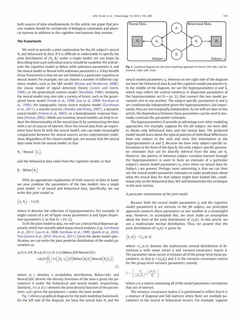
Fig. 1. Graphical diagram for the joint modeling approach of neural (left side) and be-havioral (right side) data.

195B.M. Turner et al. / NeuroImage 72 (2013) 193–206

both sources of data simultaneously. In this article, we argue that pro-cess models should be considerate of biological constraints and physi-cal systems in addition to the cognitive mechanisms they assume.

The framework

We wish to provide a joint explanation for the jth subject's neuralNj and behavioral Bj data. If it is difficult or undesirable to specify thejoint distribution of (Nj, Bj) under a single model, we can begin bydescribing how each individual source should bemodeled.Wewill de-note the cognitive model as Behav with unknown parameters θ, andthe neural model as Neural with unknown parameters δ. A key benefitof our framework is that we are not limited to a particular cognitive orneural model. For example, we can choose a number of different cog-nitive models, such as the LBA model (Brown and Heathcote, 2008),the classic model of signal detection theory (Green and Swets,1966), or the generalized context model (Nosofsky, 1986). Similarly,the neural model may also take a variety of forms, such as the gener-alized linear model (Frank et al., 1998; Guo et al., 2008; Kershaw etal., 1999), the topographic latent source analysis model (Gershmanet al., 2011), a wavelet process (Flandin and Penny, 2007), a dynamiccausal model (Friston et al., 2003), or a hemodynamic response func-tion (Friston, 2002). While not essential, neural models can help to re-duce the dimensionality of the neural dataNj by summarizing the datawith a set of sources of interest. Once the neural data from an experi-ment have been fit with the neural model, one can make meaningfulcomparisons between the neural sources across experimental condi-tions. Regardless of the chosen model pair, we assume that the neuraldata come from the neural model, so that

Nj eNeural δj� �

;

and the behavioral data come from the cognitive model, so that

Bj e Behav θj� �

:

With an appropriate explanation of both sources of data in hand,we now combine the parameters of the two models into a singlejoint model M of neural and behavioral data. Specifically, we canwrite this joint model as

δj; θj� � eM Ωð Þ:

where Ω denotes the collection of hyperparameters. For example, Ωmight consist of a set of hyper mean parameters ϕ and hyper disper-sion parameters Σ so that Ω={Φ, Σ}.

To fit the jointmodel to data, we will use a hierarchical Bayesian ap-proach, which has recently aidedmany neural analyses (e.g., Gershmanet al., 2011; Guo et al., 2008; Kershaw et al., 1999; Quirós et al., 2010;Van Gerven et al., 2010; Wu et al., 2011). Given the above model spec-ification, we can write the joint posterior distribution of the model pa-rameters as

pðΩ; θ; δ N;Bj Þ∝p Ωð ÞMð θ; δð Þ Ωj ÞBehavðB θj ÞNeuralðN δj Þ

∝p Ωð Þ∏J

j¼1M θj; δj

� ����� �Behav Bj

���θj� �Neural Nj

���δj� �h i;

ð1Þ

where p(·) denotes a probability distribution, Behav(a|b) andNeural(a|b) denote the density functions of the data a given the pa-rameters b under the behavioral and neural model, respectively.Similarly,M a; bð Þ cj Þð denotes the joint density function of the param-eters (a,b) given the parameters c under the joint model.

Fig. 1 shows a graphical diagram for the jointmodeling framework.On the left side of the diagram, we have the neural data Nj and the

neural model parameters δj, whereas on the right side of the diagramwe have the behavioral data Bj and the cognitive model parameters θj.In the middle of the diagram, we see the hyperparameters ϕ and Σ,which may reflect the central tendency or dispersion parameters ofthe hyperparameter set Ω={ϕ, Σ}, that connect the two model pa-rameter sets to one another. The subject-specific parameters θj and δjare conditionally independent given the hyperparameters, but impor-tantly, they are notmarginally independent. Aswewill see later in thisarticle, the dependency between these parameters can be used tomu-tually constrain the parameter estimates.

The hyperparametersΩ provide an advantage over othermodelingapproaches. For example, suppose for the jth subject, we were ableto obtain only behavioral data, and not neural data. The proposedmodel would learn about the typical patterns of individual differencesfrom one subject to the next and store this information in thehyperparameters ϕ and Σ. Because we have only subject-specific in-formation in the form of the data Bj, the only subject-specific parame-ter estimates that can be directly inferred from the data are θj.However, the pattern of between-subject variation learned throughthe hyperparameters is used to form an estimate of a particularsubject's neural model parameters δj, even when no neural data forSubject j are present. Perhaps more interesting is that we can thenuse the neural model parameter estimates to make predictions aboutwhat the neural data for that subject might have looked like, condi-tional only on the behavioral data.Wewill demonstrate this techniquein the next section.

A particular instantiation of the joint model

Because both the neural model parameters δj and the cognitivemodel parameters θj are intrinsic to the jth subject, our principledapproach connects these parameters to one another in a meaningfulway. However, to accomplish this, we must make an assumptionabout the form of the joint distribution of (δj,θj). In this article, weuse a multivariate normal distribution. Thus, we assume that thejoint distribution of (δj,θj) is given by

δj; θj� � eN p ϕ;Σð Þ;

where N p a; bð Þ denotes the multivariate normal distribution of di-mension p with mean vector a and variance-covariance matrix b.The parameter mean vector ϕ contains all of the group-level mean pa-rameters, so that ϕ={δμ,θμ} and Σ is the variance–covariance matrixfor the group-level variance parameters, namely

where ρ is a matrix containing all of the model parameter correlationsthat are of interest.

The variance–covariance matrix Σ is partitioned to reflect that it isa mixture of diagonal and full matrices when there are multiple pa-rameters in the neural or behavioral vectors. For example, suppose

"New" "Old"

d/2 + b

0 d/2 d

Familiarity

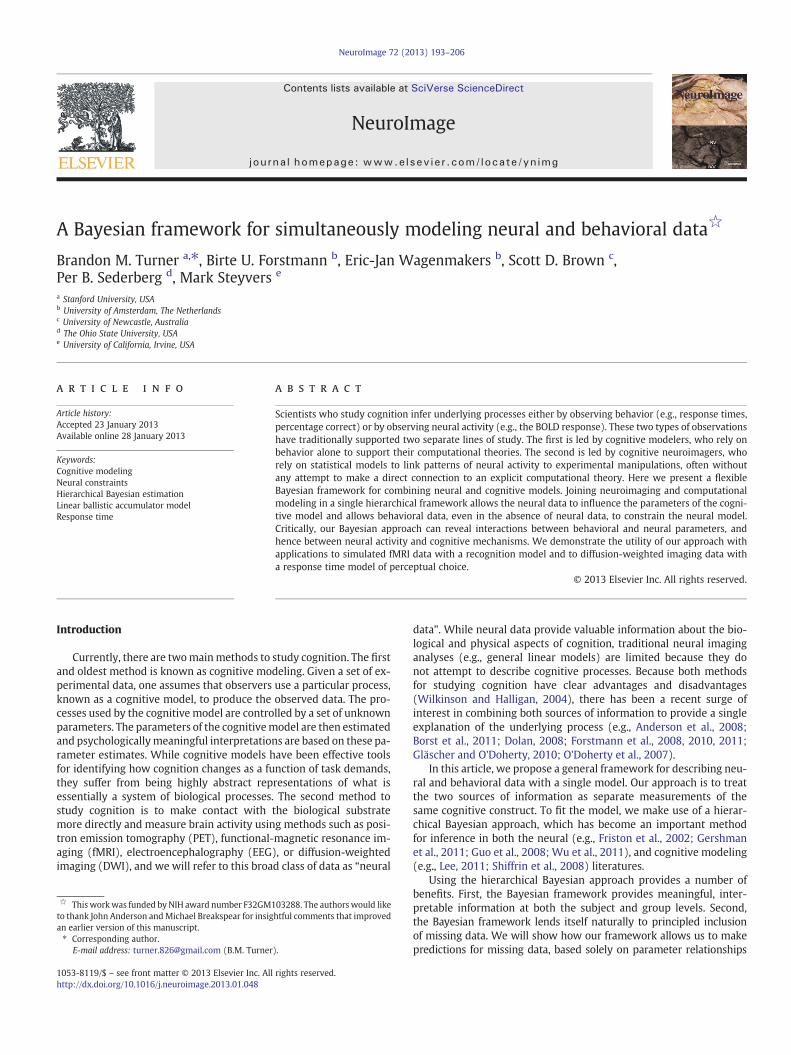
Fig. 2. The classic equal-variance model of signal detection theory. Representations fortargets and distractors are represented as equal-variance Gaussian distributions, sepa-rated by a distance d, known as the discriminability parameter. A criterion, shown asthe vertical dashed line, is used to determine the response. Deviation from the optimalcriterion placement at d/2 is a bias, and is measured by the parameter b.

196 B.M. Turner et al. / NeuroImage 72 (2013) 193–206

our neural and cognitive models contain three parameters per subject(i.e., δj and θj each have three elements). We can then write the par-tition as

δ2σ ¼δ2σ ;1 0 00 δ2σ ;2 00 0 δ2σ ;3

264375;

where δσ,1 denotes the hyper standard deviation for the first modelparameter set. We can constrain off-diagonal elements to be zero ifwe are not interested in quantifying the correlations between a setof model parameters. The relationships between the model parame-ters will still be inferred by the model because the dependenciesexist in the likelihood function. Thus, we can still detect trade-offsthat exist between model parameters by examining their joint poste-rior distribution once the model has been fit to the data. On the otherhand, we write the partition that combines the neural and cognitivemodel parameters as

ρδσθσ ¼ρ11δσ ;1θσ ;1 ρ12δσ ;1θσ ;2 ρ13δσ ;1θσ ;3

ρ21δσ ;2θσ ;1 ρ22δσ ;2θσ ;2 ρ23δσ ;2θσ ;3

ρ31δσ ;3θσ ;1 ρ32δσ ;3θσ ;2 ρ33δσ ;3θσ ;3

264375:

Specifying the model in this way allows us to infer directly the de-gree to which cognitive model parameters are related to which neuralmodel parameters. However, one can also choose to reduce the numberof model parameters by constraining some elements of this variance–covariance matrix to be equal to zero (e.g., ρ33=0).

Note that we are not restricted to a multivariate normal distributionin our specification ofM Ωð Þ. We chose themultivariate normal becauseit provides a convenient distributionwith infinite supportwith clear pa-rameter interpretations. For example, the correlation parameters ρ pro-vide a quantification of magnitude and direction of the relationshipbetween pairs ofmodel parameters. Despite this, the use ofmultivariatenormality may not be appropriate in some situations. For example,when the support of a parameter is bounded, it may not be appropriateto assume an infinite support via the normal distribution. However, themultivariate normal distribution can easily be truncated to accommo-date various parameter space supports and provides a convenient wayto assess the relationship between the neural model parameters andthe cognitive model parameters. As an alternative, transformationssuch as the log or logit produce infinite parameter supports.

Fitting the joint model to recognition and fMRI data

Simulation study

In order to highlight the advantages of our approachwe conducteda simulation study in which we generated data from the joint modelso that the neural side (i.e., the left side of Fig. 1) consisted of fMRIscans and the behavioral side (i.e., the right side of Fig. 1) consistedof data from a recognition memory task. The simulation was designedto mimic a typical recognition memory experiment in which, duringa study phase, a subject is provided with a single set of items(e.g., words or pictures) and is asked to commit the items to memory.Then, during a test phase, subjects are presented with items thateither were (a target) or were not (a distractor) on the previouslystudied list. The subjects are then asked to respond either “old”, indi-cating that the presented item was on the previously studied list, or“new”, indicating that the presented item was not on the previouslystudied list. Given the two types of words (i.e., targets or distractors)and the two types of responses (i.e., “old” or “new”), there are onlyfour possible outcomes for each trial. However, it is sufficient tofocus on only two of these possibilities. Specifically, we record thenumber of hits, which occur when an “old” response is given to

targets, and the number of false alarms, which occur when a “old” re-sponse is given to a distractor.

To obtain the neural data, we assume that single-trial regressioncoefficients (often called betas) have already been extracted from asequence of fMRI scans for each subject on each trial (Mumford etal., 2012). For simplicity and visualization purposes, we assume thatthe betas form a two dimensional map (i.e., a single slice), but onecould easily extend the model to account for slices covering thewhole brain. Subjects performed this recognition memory task for 100trials. The test list consisted of 50 targets and 50 distractors. Thus, foreach subject, we obtain 100 parametric maps (i.e., sets of single-trialbeta estimates) and 100 responses (i.e., one response and one scan foreach presented stimulus).

To explain the full model, we first describe how onemight accountfor both the behavioral and neural data and then explain how the fullmodel generates data for each subject.

The cognitive model

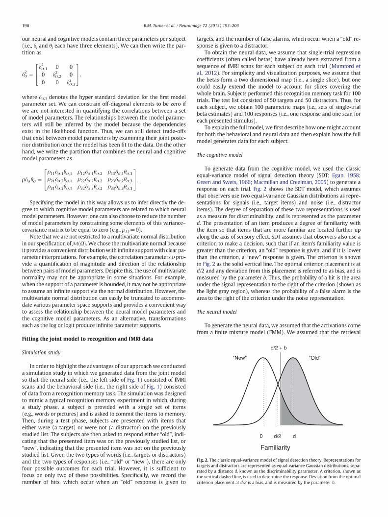
To generate data from the cognitive model, we used the classicequal-variance model of signal detection theory (SDT; Egan, 1958;Green and Swets, 1966; Macmillan and Creelman, 2005) to generate aresponse on each trial. Fig. 2 shows the SDT model, which assumesthat observers use two equal-variance Gaussian distributions as repre-sentations for signals (i.e., target items) and noise (i.e., distractoritems). The degree of separation of these two representations is usedas a measure for discriminability, and is represented as the parameterd. The presentation of an item produces a degree of familiarity withthe item so that items that are more familiar are located further upalong the axis of sensory effect. SDT assumes that observers also use acriterion to make a decision, such that if an item's familiarity value isgreater than the criterion, an “old” response is given, and if it is lowerthan the criterion, a “new” response is given. The criterion is shownin Fig. 2 as the solid vertical line. The optimal criterion placement is atd/2 and any deviation from this placement is referred to as bias, and ismeasured by the parameter b. Thus, the probability of a hit is the areaunder the signal representation to the right of the criterion (shown asthe light gray region), whereas the probability of a false alarm is thearea to the right of the criterion under the noise representation.

The neural model

To generate the neural data, we assumed that the activations comefrom a finite mixture model (FMM). We assumed that the retrieval

−2 −1 0 1 2

−2

−1

01

2

−2 −1 0 1 2

−2

−1

01

2

1

2

3

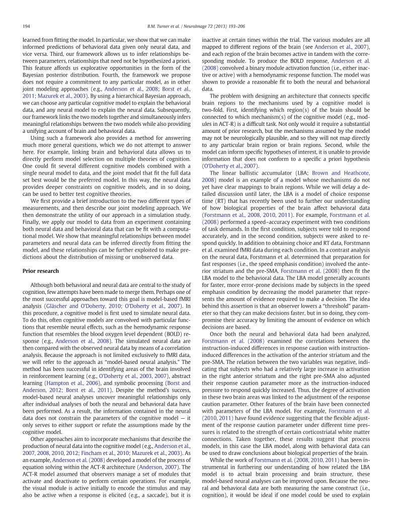
Fig. 3. An example of how the neural model explains the raw data (left panel) through a finite mixture of normal distributions (right panel). Voxels that have larger degrees ofactivity are translated to regions of larger activation in the corresponding source of the normal mixture model.

1 We set the variance of the proposal to 0.001, chose the optimal setting for the scal-ing parameter, and did not employ a migration step.

197B.M. Turner et al. / NeuroImage 72 (2013) 193–206

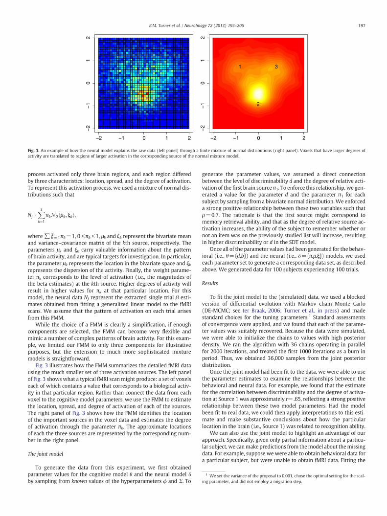
process activated only three brain regions, and each region differedby three characteristics: location, spread, and the degree of activation.To represent this activation process, we used a mixture of normal dis-tributions such that

Nj eX3k¼1

πkN 2 μk; ξkð Þ;

where∑k=13 πk=1, 0≤πk≤1, μk and ξk represent the bivariate mean

and variance–covariance matrix of the kth source, respectively. Theparameters μk and ξk carry valuable information about the patternof brain activity, and are typical targets for investigation. In particular,the parameter μk represents the location in the bivariate space and ξkrepresents the dispersion of the activity. Finally, the weight parame-ter πk corresponds to the level of activation (i.e., the magnitudes ofthe beta estimates) at the kth source. Higher degrees of activity willresult in higher values for πk at that particular location. For thismodel, the neural data Nj represent the extracted single trial β esti-mates obtained from fitting a generalized linear model to the fMRIscans. We assume that the pattern of activation on each trial arisesfrom this FMM.

While the choice of a FMM is clearly a simplification, if enoughcomponents are selected, the FMM can become very flexible andmimic a number of complex patterns of brain activity. For this exam-ple, we limited our FMM to only three components for illustrativepurposes, but the extension to much more sophisticated mixturemodels is straightforward.

Fig. 3 illustrates how the FMM summarizes the detailed fMRI datausing the much smaller set of three activation sources. The left panelof Fig. 3 shows what a typical fMRI scanmight produce: a set of voxelseach of which contains a value that corresponds to a biological activ-ity in that particular region. Rather than connect the data from eachvoxel to the cognitive model parameters, we use the FMM to estimatethe location, spread, and degree of activation of each of the sources.The right panel of Fig. 3 shows how the FMM identifies the locationof the important sources in the voxel data and estimates the degreeof activation through the parameter πk. The approximate locationsof each the three sources are represented by the corresponding num-ber in the right panel.

The joint model

To generate the data from this experiment, we first obtainedparameter values for the cognitive model θ and the neural model δby sampling from known values of the hyperparameters ϕ and Σ. To

generate the parameter values, we assumed a direct connectionbetween the level of discriminability d and the degree of relative acti-vation of the first brain source π1. To enforce this relationship, we gen-erated a value for the parameter d and the parameter π1 for eachsubject by sampling from a bivariate normal distribution.We enforceda strong positive relationship between these two variables such thatρ=0.7. The rationale is that the first source might correspond tomemory retrieval ability, and that as the degree of relative source ac-tivation increases, the ability of the subject to remember whether ornot an item was on the previously studied list will increase, resultingin higher discriminability or d in the SDT model.

Once all of the parameter values had been generated for the behav-ioral (i.e., θ={d,b}) and the neural (i.e., δ={π,μ,ξ}) models, we usedeach parameter set to generate a corresponding data set, as describedabove. We generated data for 100 subjects experiencing 100 trials.

Results

To fit the joint model to the (simulated) data, we used a blockedversion of differential evolution with Markov chain Monte Carlo(DE-MCMC; see ter Braak, 2006; Turner et al., in press) and madestandard choices for the tuning parameters.1 Standard assessmentsof convergence were applied, and we found that each of the parame-ter values was suitably recovered. Because the data were simulated,we were able to initialize the chains to values with high posteriordensity. We ran the algorithm with 36 chains operating in parallelfor 2000 iterations, and treated the first 1000 iterations as a burn inperiod. Thus, we obtained 36,000 samples from the joint posteriordistribution.

Once the joint model had been fit to the data, we were able to usethe parameter estimates to examine the relationships between thebehavioral and neural data. For example, we found that the estimatefor the correlation between discriminability and the degree of activa-tion at Source 1 was approximately r=.65, reflecting a strong positiverelationship between these two model parameters. Had the modelbeen fit to real data, we could then apply interpretations to this esti-mate and make substantive conclusions about how the particularlocation in the brain (i.e., Source 1) was related to recognition ability.

We can also use the joint model to highlight an advantage of ourapproach. Specifically, given only partial information about a particu-lar subject, we canmake predictions from themodel about themissingdata. For example, suppose we were able to obtain behavioral data fora particular subject, but were unable to obtain fMRI data. Fitting the

198 B.M. Turner et al. / NeuroImage 72 (2013) 193–206

joint model to the data would allow us to generate a predictive distri-bution for the pattern of source activation based on the relationshipsbetween the behavioral and neural models inferred from the groupdata. We can then take the predicted pattern of source activation fromthe neural model to produce a predicted pattern of activation at thevoxel level. This process can even be reversed so that if we were ableto obtain only neural data for a particular subject, we could makepredictions about what the hit and false alarm rates could have been,conditional on the pattern of brain activity observed in the fMRI scan.

To illustrate this feature of the model, we also fit the joint model tothe data of four subjects having only partial observations. Specifically,two of the subjects were simulated so that only neural data wereobtained in the form of a fMRI scan and the other two subjects weresimulated to have only behavioral data (i.e., the number of hit andfalse alarms). The goal was then to make predictions for the datathat were not obtained for each of these subjects.

Predicting behavioral data from neural dataFor the first two partially observed subjects, we obtained only

neural data. The neural data were assumed to have been gatheredin the same way as all of the other subjects (as described above).The model was fit to the full data set including the partially observedsubjects and we used this information to obtain predictions about thedistribution of behavioral data that we would have obtained, had wecollected the behavioral data.

Because we use a Bayesian approach to fitting our joint model to thedata, we can easilymake predictions about unobserved data. Themodelfirst obtains information from the neural data by estimating the

Fig. 4. Two examples of predictions made from the joint model given only neural data. Thelow Source 1 activation and the bottom row represents a subject with high Source 1 activahavioral data). The middle panel plots the joint distribution of the activation of Source 1red vertical dashed lines represent the estimated degree of Source 1 activation in the correhit (y-axis) and false alarm (x-axis) rates made by the model along with the mean predictiorow. Reference lines of d={0,1,2} are also show in the right panels.

parameters of the neural model. Then, themodel sends the informationcontained in the parameter estimates up to the hyperparameters ϕ andΣ. The hyperparameters have information about the structural relation-ships between the neural model parameters and the cognitive modelparameters, and this information is driven by the subjects who werefully observed. Using the information contained in ϕ and Σ, we canthen make predictions about the parameter estimates for the cognitivemodel, in this case the SDT model parameters θ={d,b}. Finally, usingthe parameter estimates for the cognitive model, we can make predic-tions about the hit and false alarm rates thatwould have been obtained,given the neural data.

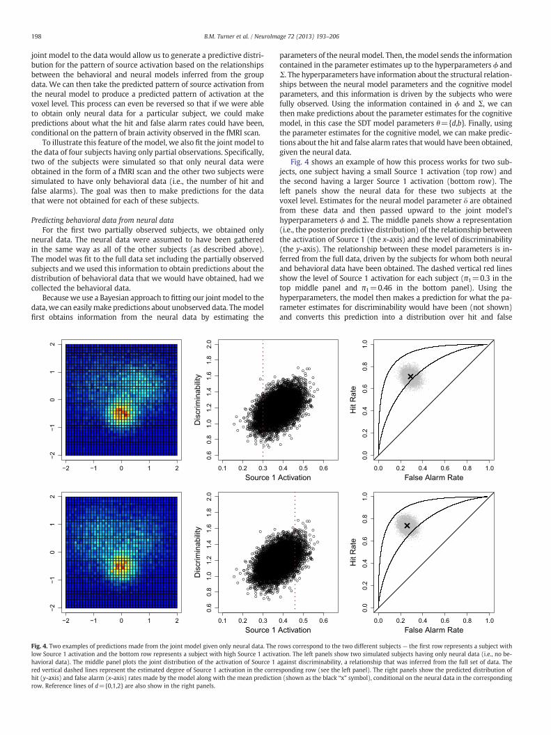
Fig. 4 shows an example of how this process works for two sub-jects, one subject having a small Source 1 activation (top row) andthe second having a larger Source 1 activation (bottom row). Theleft panels show the neural data for these two subjects at thevoxel level. Estimates for the neural model parameter δ are obtainedfrom these data and then passed upward to the joint model'shyperparameters ϕ and Σ. The middle panels show a representation(i.e., the posterior predictive distribution) of the relationship betweenthe activation of Source 1 (the x-axis) and the level of discriminability(the y-axis). The relationship between these model parameters is in-ferred from the full data, driven by the subjects for whom both neuraland behavioral data have been obtained. The dashed vertical red linesshow the level of Source 1 activation for each subject (π1=0.3 in thetop middle panel and π1=0.46 in the bottom panel). Using thehyperparameters, the model then makes a prediction for what the pa-rameter estimates for discriminability would have been (not shown)and converts this prediction into a distribution over hit and false

rows correspond to the two different subjects — the first row represents a subject withtion. The left panels show two simulated subjects having only neural data (i.e., no be-against discriminability, a relationship that was inferred from the full set of data. Thesponding row (see the left panel). The right panels show the predicted distribution ofn (shown as the black “x” symbol), conditional on the neural data in the corresponding

199B.M. Turner et al. / NeuroImage 72 (2013) 193–206

alarm rates. The predicted behavioral data are shown as the gray cloudsin the right panels of Fig. 4. As a guide, reference lines corresponding tod=0 (the diagonal line), d=1 (themiddle curved line), and d=2 (theline with the sharpest curve) are shown and themeans of the predictedhit and false alarm rates are shown as the black “x” symbols. The figureshows that for the subject with a smaller Source 1 activation, themodelpredicts that that subject will tend to have lower discriminability thanthe subject with a larger Source 1 activation.

Predicting neural data from behavioral dataWe also examined the model predictions for neural data, given

only behavioral data. The ability of the joint model to make these pre-dictions is important from a cost and ethical point of view, becauseneural data can often be expensive and time consuming to obtain(e.g., fMRI). The ability to predict neural activity from behavioraldata alone could be particularly useful in the clinical setting, wherethe exact structure of affected brain regions in unhealthy subjectscan be difficult to pinpoint. Furthermore, the joint modeling frame-work could be used on preliminary data to aid in designing newexperiments that better identify these affected regions or better testpsychological theory (Myung and Pitt, 2009).

To examine the model predictions, we fit the joint model to thefull data set, but included two subjects for whom only behavioraldata were obtained. As in the above example, the model can easilymake predictions for neural data given only the behavioral dataafter uncovering the relationships between the neural and cognitivemodel parameters. When only behavioral data have been observed,the information is passed in the opposite direction as described inthe previous example.

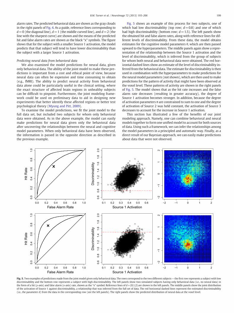
Fig. 5. Two examples of predictionsmade from the jointmodel given only behavioral data. Thediscriminability and the bottom row represents a subject with high discriminability. The leftthe form of a hit (y-axis) and false alarm (x-axis) rate, shown as the “x” symbol. Reference lineof the activation of Source 1 against discriminability, a relationship that was inferred from the(i.e., the parameter d) from the data in the corresponding row (see the left panels). The right p

Fig. 5 shows an example of this process for two subjects, one ofwhich had low discriminability (top row; d=0.8) and one of whichhad high discriminability (bottom row; d=1.5). The left panels showthe obtained hit and false alarm rates, alongwith reference lines for dif-ferent levels of discriminability. From these data, the model obtainsestimates for the cognitive model parameters θ, which are then passedupward to the hyperparameters. Themiddle panels again show a repre-sentation of the relationship between the Source 1 activation and thelevel of discriminability, which is inferred from the group of subjectsfor whom both neural and behavioral data were obtained. The red hor-izontal dashed lines show an estimate of the level of discriminability in-ferred from the behavioral data. The estimate for discriminability is thenused in combination with the hyperparameters to make predictions forthe neuralmodel parameters (not shown),which are then used tomakepredictions for the pattern of activity that might have been observed atthe voxel level. These patterns of activity are shown in the right panelsof Fig. 5. The model shows that as the hit rate increases and the falsealarm rate decreases (resulting in greater accuracy), the degree ofSource 1 activation becomes stronger. In addition, because the degreeof activation parameters π are constrained to sum to one and the degreeof activation of Source 2 was held constant, the activation of Source 3decreases to account for the increase in Source 1 activation.

This section has illustrated a few of the benefits of our jointmodeling approach. Namely, one can combine behavioral and neuralmodels together to formone unifiedmodel to account for both sourcesof data. Using such a framework, we can infer the relationships amongthe model parameters in a principled and automatic way. Finally, as adirect result of our Bayesian approach, we can easily make predictionsabout data that were not observed.

rows correspond to the two different subjects— the first row represents a subjectwith lowpanels show two simulated subjects having only behavioral data (i.e., no neural data) ins of d={0,1,2} are shown in the left panels. The middle panels show the joint distributionfull set of data. The red horizontal dashed lines represent the estimated discriminabilityanels show the predicted distribution of neural data at the voxel level.

Evi

denc

e

A

k1~CU(0, A)

d1~N(v1, s) A

k2~CU(0, A)

d2~N(v2, s)

Response Time

b b

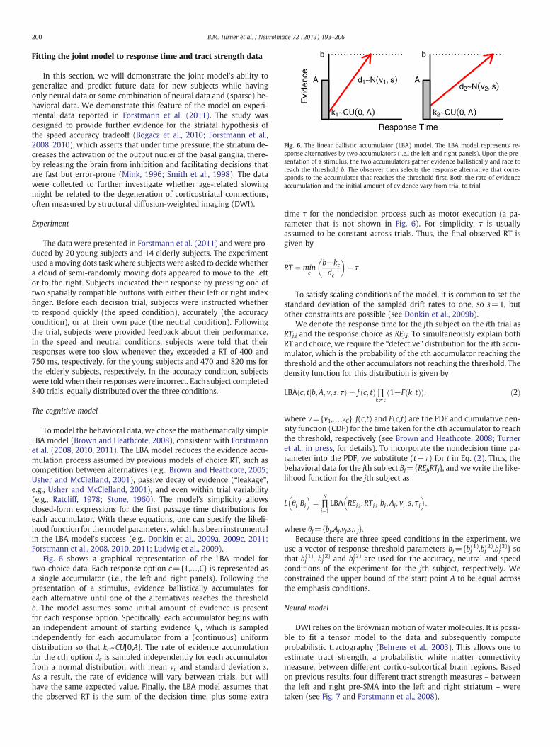
Fig. 6. The linear ballistic accumulator (LBA) model. The LBA model represents re-sponse alternatives by two accumulators (i.e., the left and right panels). Upon the pre-sentation of a stimulus, the two accumulators gather evidence ballistically and race toreach the threshold b. The observer then selects the response alternative that corre-sponds to the accumulator that reaches the threshold first. Both the rate of evidenceaccumulation and the initial amount of evidence vary from trial to trial.

200 B.M. Turner et al. / NeuroImage 72 (2013) 193–206

Fitting the joint model to response time and tract strength data

In this section, we will demonstrate the joint model's ability togeneralize and predict future data for new subjects while havingonly neural data or some combination of neural data and (sparse) be-havioral data. We demonstrate this feature of the model on experi-mental data reported in Forstmann et al. (2011). The study wasdesigned to provide further evidence for the striatal hypothesis ofthe speed accuracy tradeoff (Bogacz et al., 2010; Forstmann et al.,2008, 2010), which asserts that under time pressure, the striatum de-creases the activation of the output nuclei of the basal ganglia, there-by releasing the brain from inhibition and facilitating decisions thatare fast but error-prone (Mink, 1996; Smith et al., 1998). The datawere collected to further investigate whether age-related slowingmight be related to the degeneration of corticostriatal connections,often measured by structural diffusion-weighted imaging (DWI).

Experiment

The data were presented in Forstmann et al. (2011) and were pro-duced by 20 young subjects and 14 elderly subjects. The experimentused amoving dots task where subjects were asked to decide whethera cloud of semi-randomly moving dots appeared to move to the leftor to the right. Subjects indicated their response by pressing one oftwo spatially compatible buttons with either their left or right indexfinger. Before each decision trial, subjects were instructed whetherto respond quickly (the speed condition), accurately (the accuracycondition), or at their own pace (the neutral condition). Followingthe trial, subjects were provided feedback about their performance.In the speed and neutral conditions, subjects were told that theirresponses were too slow whenever they exceeded a RT of 400 and750 ms, respectively, for the young subjects and 470 and 820 ms forthe elderly subjects, respectively. In the accuracy condition, subjectswere told when their responses were incorrect. Each subject completed840 trials, equally distributed over the three conditions.

The cognitive model

Tomodel the behavioral data, we chose themathematically simpleLBA model (Brown and Heathcote, 2008), consistent with Forstmannet al. (2008, 2010, 2011). The LBA model reduces the evidence accu-mulation process assumed by previous models of choice RT, such ascompetition between alternatives (e.g., Brown and Heathcote, 2005;Usher and McClelland, 2001), passive decay of evidence (“leakage”,e.g., Usher and McClelland, 2001), and even within trial variability(e.g., Ratcliff, 1978; Stone, 1960). The model's simplicity allowsclosed-form expressions for the first passage time distributions foreach accumulator. With these equations, one can specify the likeli-hood function for themodel parameters, which has been instrumentalin the LBA model's success (e.g., Donkin et al., 2009a, 2009c, 2011;Forstmann et al., 2008, 2010, 2011; Ludwig et al., 2009).

Fig. 6 shows a graphical representation of the LBA model fortwo-choice data. Each response option c={1,…,C} is represented asa single accumulator (i.e., the left and right panels). Following thepresentation of a stimulus, evidence ballistically accumulates foreach alternative until one of the alternatives reaches the thresholdb. The model assumes some initial amount of evidence is presentfor each response option. Specifically, each accumulator begins withan independent amount of starting evidence kc, which is sampledindependently for each accumulator from a (continuous) uniformdistribution so that kc~CU[0,A]. The rate of evidence accumulationfor the cth option dc is sampled independently for each accumulatorfrom a normal distribution with mean vc and standard deviation s.As a result, the rate of evidence will vary between trials, but willhave the same expected value. Finally, the LBA model assumes thatthe observed RT is the sum of the decision time, plus some extra

time τ for the nondecision process such as motor execution (a pa-rameter that is not shown in Fig. 6). For simplicity, τ is usuallyassumed to be constant across trials. Thus, the final observed RT isgiven by

RT ¼ minc

b−kcdc

� �þ τ:

To satisfy scaling conditions of the model, it is common to set thestandard deviation of the sampled drift rates to one, so s=1, butother constraints are possible (see Donkin et al., 2009b).

We denote the response time for the jth subject on the ith trial asRTj,i and the response choice as REj,i. To simultaneously explain bothRT and choice, we require the “defective” distribution for the ith accu-mulator, which is the probability of the cth accumulator reaching thethreshold and the other accumulators not reaching the threshold. Thedensity function for this distribution is given by

LBAðc; t b;A; v; s; τj Þ ¼ f c; tð Þ∏k≠c

1−F k; tð Þð Þ; ð2Þ

where v={v1,…,vC}, f(c,t) and F(c,t) are the PDF and cumulative den-sity function (CDF) for the time taken for the cth accumulator to reachthe threshold, respectively (see Brown and Heathcote, 2008; Turneret al., in press, for details). To incorporate the nondecision time pa-rameter into the PDF, we substitute (t−τ) for t in Eq. (2). Thus, thebehavioral data for the jth subject Bj={REj,RTj}, and wewrite the like-lihood function for the jth subject as

L�θj Bj

��� � ¼ ∏N

i¼1LBA REj;i;RTj;i bj;Aj; vj; s; τj

��� �;

�

where θj={bj,Aj,vj,s,τj}.Because there are three speed conditions in the experiment, we

use a vector of response threshold parameters bj={bj(1),bj(2),bj(3)} sothat bj(1), bj(2) and bj

(3) are used for the accuracy, neutral and speedconditions of the experiment for the jth subject, respectively. Weconstrained the upper bound of the start point A to be equal acrossthe emphasis conditions.

Neural model

DWI relies on the Brownian motion of water molecules. It is possi-ble to fit a tensor model to the data and subsequently computeprobabilistic tractography (Behrens et al., 2003). This allows one toestimate tract strength, a probabilistic white matter connectivitymeasure, between different cortico-subcortical brain regions. Basedon previous results, four different tract strength measures – betweenthe left and right pre-SMA into the left and right striatum – weretaken (see Fig. 7 and Forstmann et al., 2008).

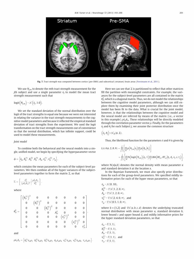
Fig. 7. Tract strength was computed between cortico (pre-SMA) and subcortical (striatum) brain areas (Forstmann et al., 2011).

201B.M. Turner et al. / NeuroImage 72 (2013) 193–206

We use Nj,m to denote themth tract strength measurement for thejth subject and use a single parameter δj to model the mean tractstrength measurement such that

logit Nj;m

� � eN δj;1:0� �

:

We set the standard deviation of the normal distribution over thelogit of the tract strengths to equal one because we were not interestedin relating the variance in the tract strength measurements to the cog-nitivemodel parameters and because it reflected the empirical standarddeviation of tract strengths from the experiment. We used the logittransformation on the tract strength measurements out of convenienceso that the normal distribution, which has infinite support, could beused to model these measurements.

Joint model

To combine both the behavioral and the neural models into a sin-gle, unified model, we begin by specifying the hyperparameter vector

ϕ ¼ δμ ; b1ð Þμ ; b 2ð Þ

μ ; b 3ð Þμ ;Aμ ; v

1ð Þμ ; v 2ð Þ

μ ; τμh i

;

which contains the mean parameters for each of the subject-level pa-rameters. We then combine all of the hyper variances of the subject-level parameters together to form the matrix Σ, so that

where

θ2σ ¼

b 1ð Þσ

� �20 0 0 0 0 0

0 b 2ð Þσ

� �20 0 0 0 0

0 0 b 3ð Þσ

� �20 0 0 0

0 0 0 A2σ 0 0 0

0 0 0 0 v 1ð Þσ

� �20 0

0 0 0 0 0 v 2ð Þσ

� �20

0 0 0 0 0 0 τ2σ

26666666666666664

37777777777777775;

and

ρδσθσ ¼ b 1ð Þσ δσρ1 b 2ð Þ

σ δσρ2 b 3ð Þσ δσρ3 Aσδσρ4 v 1ð Þ

σ δσρ5 v 2ð Þσ δσρ6 τσδσρ7

h i:

Here we can see that Σ is partitioned to reflect that other matricesfill the partition with meaningful constraints. For example, the vari-ances for the subject-level parameters are all contained in the matrixθσ2, which is a diagonal matrix. Thus, we do notmodel the relationshipsbetween the cognitive model parameters, although we can still ex-plore them by examining their joint posterior distribution once themodel has been fit to the data. What is crucial for the joint model,however, is that the relationships between the cognitive model andthe neural model are inferred by means of the matrix (i.e., a vectorin this example) ρδσθσ. These relationships will be directly modeledthrough the correlation parameter vector ρ. Finally, for the parametersδj and θj for each Subject j, we assume the common structure

δj; θj� �

∼N 8 ϕ;Σð Þ:

Thus, the likelihood function for the parameters δ and θ is given by

Lðδ; θ ϕ;Σ;B;Nj Þ ¼ ∏J

j¼1

"∏mp�Nj;m δj

��� �∏ip�Bj;i θj��� �#

¼ ∏J

j¼1∏mN�logit Nj;m

� �δj;1��� �

∏iLBA

�REj;i;RTj;i bj;Aj; vj; s; τj

��� �#;

"

where N(x|a,b) denotes the normal density with mean parameter aand standard deviation b at the location x.

In the Bayesian framework, we must also specify prior distribu-tions for each of the group-level parameters. We specified mildly in-formative priors for each of the hyper mean parameters, so that

δμ eN 0;10ð Þ;

b kð Þμ e T N 1;2;0;∞ð Þ;

Aμ e T N 1;2;0;∞ð Þ;

v cð Þμ e T N 2;4;0;∞ð Þ; and

τμ e T N 0:5;1;0;∞ð Þ;

where k={1,2} and TN a; b; c;dð Þ denotes the underlying truncatednormal distribution with mean parameter a, standard deviation b,lower bound c and upper bound d, and mildly informative priors forthe hyper standard deviation parameters, so that

δσ e Γ 1;1ð Þ;b kð Þσ e Γ 1;1ð Þ;

Aσ e Γ 1;1ð Þ;v cð Þσ e Γ 1;1ð Þ; and

τσ e Γ 1;1ð Þ:

202 B.M. Turner et al. / NeuroImage 72 (2013) 193–206

Because we wanted to avoid any speculation about the relation-ships between the behavioral and neural model parameters, we spec-ified noninformative priors for each of the correlation parameters,such that

ρ e CU −1;1ð Þ:

Specifying the model in this way allows for easy computationof the Bayes factor via the Savage–Dickey density ratio (see Dickey,1971; Dickey and Lientz, 1970; Friston and Penny, 2011; Wetzelset al., 2010).

Given the priors listed above, the full joint posterior distributionfor the model parameters is given by

pðδ; θ;ϕ;Σ B;Nj Þ∝Lðδ; θ ϕ;Σ;B;Nj Þ∏J

j¼1p

δj; θjh i⊤���ϕ;Σ!p ϕð Þp Σð Þ

∝Lðδ; θ ϕ;Σ;B;Nj Þ∏J

j¼1p δj; θjh i⊤���ϕ;Σ!p θμ

� �p δμ� �

p θσð Þp δσð Þp ρð Þ;

where θμ={bμ(1),bμ(2),bμ(3),Aμ,vμ(1),vμ(2),τμ}.

Results

To fit the joint model to the data, we again used a blocked versionof DE-MCMC with the same choices as above for the tuning parame-ters. We used the DE local-to-best method to obtain starting pointswith high posterior density (Turner and Sederberg, 2012). We ranthe algorithm with 24 chains operating in parallel for 5000 iterations,and treated the first 1000 iterations as a burn in period. Thus, weobtained 96,000 samples from the joint posterior distribution.

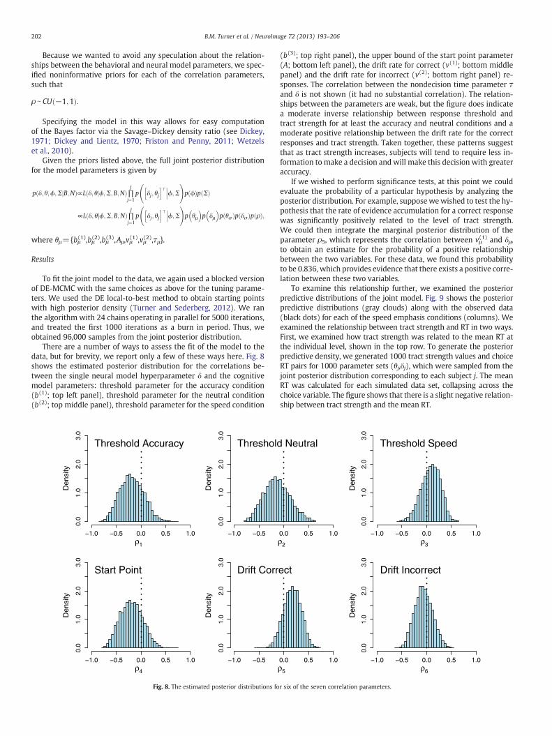
There are a number of ways to assess the fit of the model to thedata, but for brevity, we report only a few of these ways here. Fig. 8shows the estimated posterior distribution for the correlations be-tween the single neural model hyperparameter δ and the cognitivemodel parameters: threshold parameter for the accuracy condition(b(1); top left panel), threshold parameter for the neutral condition(b(2); top middle panel), threshold parameter for the speed condition

Den

sity

−1.0 −0.5 0.0 0.5 1.0

0.0

1.0

2.0

3.0

ρ1

Threshold Accuracy

−1.0 −0.5

0.0

1.0

2.0

3.0

Threshold

Den

sity

Den

sity

Den

sity

−1.0 −0.5 0.0 0.5 1.0

0.0

1.0

2.0

3.0

ρ4

Start Point

−1.0 −0.5

0.0

1.0

2.0

3.0

Drift Corr

Fig. 8. The estimated posterior distributions fo

(b(3); top right panel), the upper bound of the start point parameter(A; bottom left panel), the drift rate for correct (v(1); bottom middlepanel) and the drift rate for incorrect (v(2); bottom right panel) re-sponses. The correlation between the nondecision time parameter τand δ is not shown (it had no substantial correlation). The relation-ships between the parameters are weak, but the figure does indicatea moderate inverse relationship between response threshold andtract strength for at least the accuracy and neutral conditions and amoderate positive relationship between the drift rate for the correctresponses and tract strength. Taken together, these patterns suggestthat as tract strength increases, subjects will tend to require less in-formation to make a decision and will make this decision with greateraccuracy.

If we wished to perform significance tests, at this point we couldevaluate the probability of a particular hypothesis by analyzing theposterior distribution. For example, suppose wewished to test the hy-pothesis that the rate of evidence accumulation for a correct responsewas significantly positively related to the level of tract strength.We could then integrate the marginal posterior distribution of theparameter ρ5, which represents the correlation between vμ

(1) and δμ,to obtain an estimate for the probability of a positive relationshipbetween the two variables. For these data, we found this probabilityto be 0.836, which provides evidence that there exists a positive corre-lation between these two variables.

To examine this relationship further, we examined the posteriorpredictive distributions of the joint model. Fig. 9 shows the posteriorpredictive distributions (gray clouds) along with the observed data(black dots) for each of the speed emphasis conditions (columns). Weexamined the relationship between tract strength and RT in two ways.First, we examined how tract strength was related to the mean RT atthe individual level, shown in the top row. To generate the posteriorpredictive density, we generated 1000 tract strength values and choiceRT pairs for 1000 parameter sets (θj,δj), which were sampled from thejoint posterior distribution corresponding to each subject j. The meanRT was calculated for each simulated data set, collapsing across thechoice variable. The figure shows that there is a slight negative relation-ship between tract strength and the mean RT.

0.0 0.5 1.0ρ2

Neutral

−1.0 −0.5 0.0 0.5 1.0

0.0

1.0

2.0

3.0

ρ3

Threshold Speed

Den

sity

Den

sity

0.0 0.5 1.0ρ5

ect

−1.0 −0.5 0.0 0.5 1.0

0.0

1.0

2.0

3.0

ρ6

Drift Incorrect

r six of the seven correlation parameters.

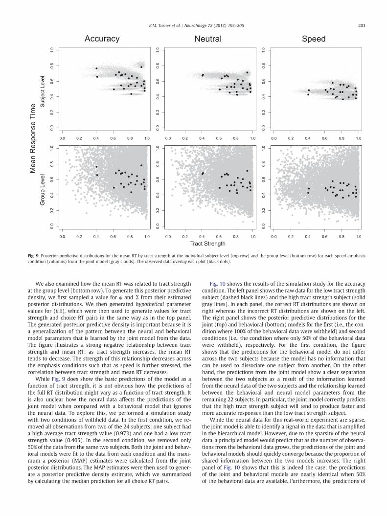
Fig. 9. Posterior predictive distributions for the mean RT by tract strength at the individual subject level (top row) and the group level (bottom row) for each speed emphasiscondition (columns) from the joint model (gray clouds). The observed data overlay each plot (black dots).

203B.M. Turner et al. / NeuroImage 72 (2013) 193–206

We also examined how the mean RT was related to tract strengthat the group level (bottom row). To generate this posterior predictivedensity, we first sampled a value for ϕ and Σ from their estimatedposterior distributions. We then generated hypothetical parametervalues for (θ,δ), which were then used to generate values for tractstrength and choice RT pairs in the same way as in the top panel.The generated posterior predictive density is important because it isa generalization of the pattern between the neural and behavioralmodel parameters that is learned by the joint model from the data.The figure illustrates a strong negative relationship between tractstrength and mean RT: as tract strength increases, the mean RTtends to decrease. The strength of this relationship decreases acrossthe emphasis conditions such that as speed is further stressed, thecorrelation between tract strength and mean RT decreases.

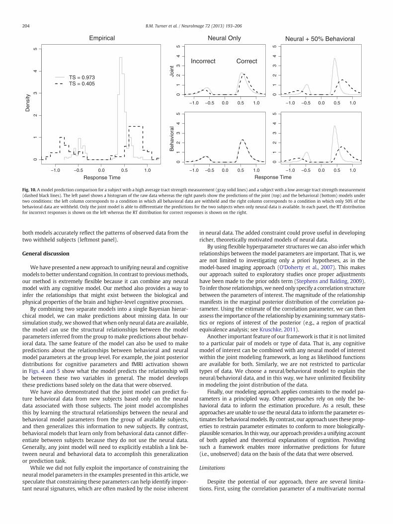
While Fig. 9 does show the basic predictions of the model as afunction of tract strength, it is not obvious how the predictions ofthe full RT distribution might vary as a function of tract strength. Itis also unclear how the neural data affects the predictions of thejoint model when compared with a behavioral model that ignoresthe neural data. To explore this, we performed a simulation studywith two conditions of withheld data. In the first condition, we re-moved all observations from two of the 24 subjects: one subject hada high average tract strength value (0.973) and one had a low tractstrength value (0.405). In the second condition, we removed only50% of the data from the same two subjects. Both the joint and behav-ioral models were fit to the data from each condition and the maxi-mum a posterior (MAP) estimates were calculated from the jointposterior distributions. The MAP estimates were then used to gener-ate a posterior predictive density estimate, which we summarizedby calculating the median prediction for all choice RT pairs.

Fig. 10 shows the results of the simulation study for the accuracycondition. The left panel shows the raw data for the low tract strengthsubject (dashed black lines) and the high tract strength subject (solidgray lines). In each panel, the correct RT distributions are shown onright whereas the incorrect RT distributions are shown on the left.The right panel shows the posterior predictive distributions for thejoint (top) and behavioral (bottom) models for the first (i.e., the con-dition where 100% of the behavioral data were withheld) and secondconditions (i.e., the condition where only 50% of the behavioral datawere withheld), respectively. For the first condition, the figureshows that the predictions for the behavioral model do not differacross the two subjects because the model has no information thatcan be used to dissociate one subject from another. On the otherhand, the predictions from the joint model show a clear separationbetween the two subjects as a result of the information learnedfrom the neural data of the two subjects and the relationship learnedbetween the behavioral and neural model parameters from theremaining 22 subjects. In particular, the joint model correctly predictsthat the high tract strength subject will tend to produce faster andmore accurate responses than the low tract strength subject.

While the neural data for this real-world experiment are sparse,the joint model is able to identify a signal in the data that is amplifiedin the hierarchical model. However, due to the sparsity of the neuraldata, a principled model would predict that as the number of observa-tions from the behavioral data grows, the predictions of the joint andbehavioral models should quickly converge because the proportion ofshared information between the two models increases. The rightpanel of Fig. 10 shows that this is indeed the case: the predictionsof the joint and behavioral models are nearly identical when 50%of the behavioral data are available. Furthermore, the predictions of

Empirical Neural Only Neural + 50% Behavioral

Den

sity

−1.0 −0.5 0.0 0.5 1.0

01

23

45

TS = 0.973TS = 0.405

Join

t

−1.0 −0.5 0.0 0.5 1.0

01

23

45

Incorrect Correct

−1.0 −0.5 0.0 0.5 1.0

01

23

45

Beh

avio

ral

−1.0 −0.5 0.0 0.5 1.0

01

23

45

−1.0 −0.5 0.0 0.5 1.0

01

23

45

Response Time Response Time

Fig. 10. Amodel prediction comparison for a subject with a high average tract strength measurement (gray solid lines) and a subject with a low average tract strength measurement(dashed black lines). The left panel shows a histogram of the raw data whereas the right panels show the predictions of the joint (top) and the behavioral (bottom) models undertwo conditions: the left column corresponds to a condition in which all behavioral data are withheld and the right column corresponds to a condition in which only 50% of thebehavioral data are withheld. Only the joint model is able to differentiate the predictions for the two subjects when only neural data is available. In each panel, the RT distributionfor incorrect responses is shown on the left whereas the RT distribution for correct responses is shown on the right.

204 B.M. Turner et al. / NeuroImage 72 (2013) 193–206

both models accurately reflect the patterns of observed data from thetwo withheld subjects (leftmost panel).

General discussion

Wehave presented a new approach to unifying neural and cognitivemodels to better understand cognition. In contrast to previousmethods,our method is extremely flexible because it can combine any neuralmodel with any cognitive model. Our method also provides a way toinfer the relationships that might exist between the biological andphysical properties of the brain and higher-level cognitive processes.

By combining two separate models into a single Bayesian hierar-chical model, we can make predictions about missing data. In oursimulation study, we showed thatwhen only neural data are available,the model can use the structural relationships between the modelparameters inferred from the group to make predictions about behav-ioral data. The same feature of the model can also be used to makepredictions about the relationships between behavioral and neuralmodel parameters at the group level. For example, the joint posteriordistributions for cognitive parameters and fMRI activation shownin Figs. 4 and 5 show what the model predicts the relationship willbe between these two variables in general. The model developsthese predictions based solely on the data that were observed.

We have also demonstrated that the joint model can predict fu-ture behavioral data from new subjects based only on the neuraldata associated with those subjects. The joint model accomplishesthis by learning the structural relationships between the neural andbehavioral model parameters from the group of available subjects,and then generalizes this information to new subjects. By contrast,behavioral models that learn only from behavioral data cannot differ-entiate between subjects because they do not use the neural data.Generally, any joint model will need to explicitly establish a link be-tween neural and behavioral data to accomplish this generalizationor prediction task.

While we did not fully exploit the importance of constraining theneural model parameters in the examples presented in this article, wespeculate that constraining these parameters can help identify impor-tant neural signatures, which are often masked by the noise inherent

in neural data. The added constraint could prove useful in developingricher, theoretically motivated models of neural data.

By using flexible hyperparameter structures we can also infer whichrelationships between the model parameters are important. That is, weare not limited to investigating only a priori hypotheses, as in themodel-based imaging approach (O'Doherty et al., 2007). This makesour approach suited to exploratory studies once proper adjustmentshave been made to the prior odds term (Stephens and Balding, 2009).To infer those relationships,we need only specify a correlation structurebetween the parameters of interest. The magnitude of the relationshipmanifests in the marginal posterior distribution of the correlation pa-rameter. Using the estimate of the correlation parameter, we can thenassess the importance of the relationship by examining summary statis-tics or regions of interest of the posterior (e.g., a region of practicalequivalence analysis; see Kruschke, 2011).

Another important feature of our framework is that it is not limitedto a particular pair of models or type of data. That is, any cognitivemodel of interest can be combined with any neural model of interestwithin the joint modeling framework, as long as likelihood functionsare available for both. Similarly, we are not restricted to particulartypes of data. We choose a neural/behavioral model to explain theneural/behavioral data, and in this way, we have unlimited flexibilityin modeling the joint distribution of the data.

Finally, our modeling approach applies constraints to the model pa-rameters in a principled way. Other approaches rely on only the be-havioral data to inform the estimation procedure. As a result, theseapproaches are unable to use the neural data to inform the parameter es-timates for behavioralmodels. By contrast, our approach uses these prop-erties to restrain parameter estimates to conform to more biologically-plausible scenarios. In thisway, our approach provides a unifying accountof both applied and theoretical explanations of cognition. Providingsuch a framework enables more informative predictions for future(i.e., unobserved) data on the basis of the data that were observed.

Limitations

Despite the potential of our approach, there are several limita-tions. First, using the correlation parameter of a multivariate normal

205B.M. Turner et al. / NeuroImage 72 (2013) 193–206

distribution may not be the best choice to understand the relation-ships between model parameters. For example, if one were interestedin causal relationships between neural sources and cognitive mecha-nisms, a discriminative approach such as structural equationmodelingor generalized linear modeling would be more useful. However, sucha model specification would still fit within the proposed framework.To do so, one would specify that say, the cognitive model parameters,are a function of the neural sources. For example, one could specify alinear relationship between the neural and cognitive model parame-ters, so that

θ ¼ δβ þ �;

where β is the standard coefficient matrix for linear regression and� specifies the error term. Here, we have defined a structural relation-ship between two latent parameters; however, one could image ascenario where the parameters δ were the neural data themselves.For example, in the data from the experiment above, one could specifythat

δ ¼ 1M

XMm¼1

Nj;m:

Here, δ becomes a deterministic node in the model and can be usedto enforce a stronger constraint on the cognitive model parameters θ. Insome preliminary studies, we have examined functional approacheslike the one described here. However, causal relationships are meantmore for confirmatory purposes (e.g., to confirm a hypothesis) whereasthe approach we present in this article is meant for exploratory pur-poses. We believe that the latter is more applicable to the generativestudy of cognition.

Another limitation comes directly from the model structure. Spe-cifically, the constraint from the group-level model parameterscould be conceived of as a limitation of our model. In some prelimi-nary studies, we have found that specifying priors for subject-levelparameters may be overly restrictive in some cases, such as whenthere are few observations at the subject-level. In this situation, be-cause little is known at the subject level, the model will resort tousing the information contained in the prior and the estimates forthe subject-level parameters may systematically differ from estimatesthat would have been obtained without the specification of a prior, aneffect known as shrinkage.

However, the way that Bayesian models handle sparse data canalso be seen as a benefit of our approach. When little is knownabout individual subjects, hierarchical Bayesian models learn a littlefrom each subject and this information is passed back and forth be-tween the group- and subject-level parameters. This same informa-tion sharing scheme is what facilitates the prediction of one sourceof data, e.g., the neural data, having only observed the behavioraldata. To remedy the problem of overly harsh prior specification,one can use more flexible distributions to characterize the distribu-tion of subject-specific model parameters. For example, one coulduse nonparametric Bayesian techniques (Gershman and Blei, 2012;Navarro et al., 2006), which allow themodel to learn themost appropri-ate representation of the distribution of subject-specific parameters.Such a flexible representation would help to attenuate the problem ofparameter shrinkage.

Throughout the manuscript, we focused on linking behavioraland neural model parameters together across subjects (see Eq. (1)).However, the joint modeling framework can be further extended tothe individual subject level, where parameters for each trial can belinked together. To do this, we need only specify that the individualtrial parameters are correlated for each individual subject. We couldthen specify a structure for the subject-specific correlation parame-ters in a three-level hierarchy. Such an extension is particularly usefulfor neural data, which are often obtained on a trial-to-trial basis.

A final limitation is in our specification of the covariance matrix Σ.For the models in this article, we set the off-diagonal elements to zerobecause the correlations among the behavioral and neural modelparameters were not theoretically important. While this particularconstraint is useful in minimizing the computational complexity as-sociated with estimating the parameters of the hierarchical model,such a constraint could have negative implications. For example, ifthe model were misspecified such that a strong (i.e., having a largemagnitude) correlation existed between the model parameters, themisspecification would manifest as a bias in the estimates of theremaining parameters. In practice, we recommend investigating avariety of model constraints so that simplifying assumptions can beproperly justified.

Conclusions

In this article, we have presented a hierarchical Bayesian frame-work for combining both neural and cognitive models into a singleunifying model. We have shown that our approach provides a num-ber of benefits over current approaches and allows for principled in-ference of the relationships between the biological properties of thebrain assessed by neuroimaging techniques and the theories of cogni-tion that are used to understand higher levels of cognitive processing.With this approach, one can investigate neural and behavioral datausing any combination of neural and cognitive models. By unifyingthe two seemingly different aspects of cognitive processing, we havepresented a step toward a better understanding of cognition.

References

Anderson, J.R., 2007. How Can the Human Mind Occur in the Physical Universe? OxfordUniversity Press, New York, NY.

Anderson, J.R., Qin, Y., Jung, K.J., Carter, C.S., 2007. Information-processing modules andtheir relative modality specificity. Cogn. Psychol. 54, 185–217.

Anderson, J.R., Carter, C.S., Fincham, J.M., Qin, Y., Rosenberg-Lee, M., S. M. R., 2008.Using fMRI to test models of complex cognition. Cogn. Sci. 32, 1323–1348.

Anderson, J.R., Betts, S., Ferris, J.L., Fincham, J.M., 2010. Neural imaging to track mentalstates. Proc. Natl. Acad. Sci. U. S. A. 107, 7018–7023.

Anderson, J.R., Fincham, J.M., Schneider, D.W., Yang, J., 2012. Using brain imaging totrack problem solving in a complex state space. NeuroImage 60, 633–643.

Behrens, T., Johansen-Berg, H., Woolrich, M.W., Smith, S.M., Wheeler-Kingshott, C.A.,Boulby, P.A., Barker, G.J., Sillery, E.L., Sheehan, K., Ciccarelli, O., Thompson, A.J.,Brady, J.M., Matthews, P.M., 2003. Non-invasive mapping f connections betweenhuman thalamus and cortex using diffusion imaging. Nat. Neurosci. 6, 750–757.

Bogacz, R., Wagenmakers, E.J., Forstmann, B.U., Nieuwenhuis, S., 2010. The neural basisof the speed–accuracy tradeoff. Trends Neurosci. 33, 10–16.

Borst, J., Anderson, J.R., 2012. Towards pinpointing the neural correlates of ACT-R:a conjunction of two model-based fMRI analyses. In: Rubwinkel, N., Drewitz, U.,van Rijn, H. (Eds.), Proceedings of the 11th International Conference on CognitiveModeling (Berlin).

Borst, J.P., Taatgen, N.A., Hedderik, V.R., 2011. Using a symbolic process model as inputfor model-based fMRI analysis: locating the neural correlates of problem statereplacement. NeuroImage 58, 137–147.

Brown, S., Heathcote, A., 2005. A ballistic model of choice response time. Psychol. Rev.112, 117–128.

Brown, S., Heathcote, A., 2008. The simplest complete model of choice reaction time:linear ballistic accumulation. Cogn. Psychol. 57, 153–178.

Dickey, J.M., 1971. The weighted likelihood ratio, linear hypotheses on normal locationparameters. Ann. Math. Stat. 42, 204–223.

Dickey, J.M., Lientz, B.P., 1970. The weighted likelihood ratio, sharp hypotheses aboutchances, the order of a Markov chain. Ann. Math. Stat. 41, 214–226.

Dolan, R.J., 2008. Neuroimaging of cognition: past, present and future. Neuron 60,496–502.

Donkin, C., Averell, L., Brown, S., Heathcote, A., 2009a. Getting more from accuracy andresponse time data: methods for fitting the linear ballistic accumulator. Behav. Res.Methods 41, 1095–1110.

Donkin, C., Brown, S., Heathcote, A., 2009b. The overconstraint of response time models:rethinking the scaling problem. Psychon. Bull. Rev. 16, 1129–1135.

Donkin, C., Heathcote, A., Brown, S., 2009c. Is the linear ballistic accumulator modelreally the simplest model of choice response times: a Bayesian model complexityanalysis. In: Howes, A., Peebles, D., Cooper, R. (Eds.), 9th International Conferenceon Cognitive Modeling — ICCM2009 (Manchester, UK).

Donkin, C., Brown, S., Heathcote, A., 2011. Drawing conclusions from choice responsetime models: a tutorial. J. Math. Psychol. 55, 140–151.

Egan, J.P., 1958. Recognition memory and the operating characteristic. Tech. Rep.AFCRC-TN-58-51. Hearing and Communication Laboratory, Indiana University,Bloomington, Indiana.

206 B.M. Turner et al. / NeuroImage 72 (2013) 193–206

Fincham, J.M., Anderson, J.R., Betts, S.A., Ferris, J.L., 2010. Using neural imaging and cog-nitive modeling to infer mental states while using and intelligent tutoring system.Proceedings of the Third International Conference on Educational Data Mining(EDM2010) (Pittsburgh, PA).

Flandin, G., Penny, W.D., 2007. Bayesian fMRI data analysis with sparse spatial basisfunctions. NeuroImage 34, 1108–1125.

Forstmann, B.U., Dutilh, G., Brown, S., Neumann, J., von Cramon, D.Y., Ridderinkhof,K.R., Wagenmakers, E.-J., 2008. Striatum and pre-SMA facilitate decision-makingunder time pressure. Proc. Natl. Acad. Sci. 105, 17538–17542.

Forstmann, B.U., Anwander, A., Schäfer, A., Neumann, J., Brown, S., Wagenmakers, E.-J.,Bogacz, R., Turner, R., 2010. Cortico-striatal connections predict control over speedand accuracy in perceptual decision making. Proc. Natl. Acad. Sci. 107, 15916–15920.

Forstmann, B.U., Tittgemeyer, M., Wagenmakers, E.-J., Derrfuss, J., Imperati, D., Brown,S., 2011. The speed-accuracy tradeoff in the elderly brain: a structural model-basedapproach. J. Neurosci. 31, 17242–17249.

Frank, L.R., Buxton, R.B., Wong, E.C., 1998. Probabilistic analysis of functional magneticresonance imaging data. Magn. Reson. Med. 39, 132–148.

Friston, K., 2002. Bayesian estimation of dynamical systems: an application to fMRI.NeuroImage 16, 513–530.

Friston, K.J., Penny, W., 2011. Post hoc Bayesian model selection. NeuroImage 56,2089–2099.

Friston, K., Penny, W., Phillips, C., Kiebel, S., Hinton, G., Ashburner, J., 2002. Classical andBayesian inference in neuroimaging. NeuroImage 16, 465–483.

Friston, K., Harisson, L., Penny, W., 2003. Dynamic causal modeling. NeuroImage 19,1273–1302.

Gershman, S.J., Blei, D.M., 2012. A tutorial on Bayesian nonparametric models. J. Math.Psychol. 56, 1–12.

Gershman, S.J., Blei, D.M., Pereira, F., Norman, K.A., 2011. A topographic latent sourcemodel for fMRI data. NeuroImage 57, 89–100.

Gläscher, J.P., O'Doherty, 2010. Model-based approaches to neuroimaging: combiningreinforcement learning theory with fMRI data. Wires Cognitive Science 1, 501–510.

Green, D.M., Swets, J.A., 1966. Signal Detection Theory and Psychophysics. Wiley Press,New York.

Guo, Y., Bowman, F.D., Kilts, C., 2008. Predicting the brain response to treatment using aBayesian hierarchical model with application to a study of schizophrenia. Hum.Brain Map. 29, 1092–1109.

Hampton, A.N., Bossaerts, P., O'Doherty, J.P., 2006. The role of the ventromedial pre-frontal cortex in abstract state-based inference during decision making in humans.J. Neurosci. 8360–8367.

Kershaw, J., Ardekani, B.A., Kanno, I., 1999. Application of Bayesian inference to fMRIdata analysis. IEEE Trans. Med. Imaging 18, 1138–1153.

Kruschke, J.K., 2011. Doing Bayesian Data Analysis: A Tutorial with R and BUGS.Academic Press, Burlington, MA.

Lee,M.D., 2011. Special issue on hierarchical Bayesianmodels. J. Math. Psychol. 55, 1–118.Ludwig, C.J.H., Farrell, S., Ellis, L.A., Gilchrist, I.D., 2009. The mechanism underlying

inhibition of saccadic return. Cogn. Psychol. 59, 180–202.Macmillan, N.A., Creelman, C.D., 2005. Detection Theory: A User's Guide. Lawrence

Erlbaum Associates, Mahwah, New Jersey.

Mazurek, M.E., Roitman, J.D., Ditterich, J., Shadlen, M.N., 2003. A role for neural integra-tors in perceptual decision making. Cereb. Cortex 13, 1257–1269.

Mink, J.W., 1996. The basal ganglia: focused selection and inhibition of competingmotor programs. Prog. Neurobiol. 50, 381–425.

Mumford, J.A., Turner, B.O., Ashby, F.G., Poldrack, R.A., 2012. Deconvolving bold activationin event-related designs for multivoxel pattern classification analyses. NeuroImage59, 2636–2643.

Myung, J.I., Pitt, M.A., 2009. Optimal experimental design for model discrimination.Psychol. Rev. 116, 499–518.

Navarro, D.J., Griffiths, T.L., Steyvers, M., Lee, M.D., 2006. Modeling individual differencesusing Dirichlet processes. J. Math. Psychol. 50, 101–122.

Nosofsky, R.M., 1986. Attention, similarity, and the identification–categorization rela-tionship. J. Exp. Psychol. Gen. 115, 39–57.

O'Doherty, J.P., Dayan, P., Friston, K., Critchley, H., Dolan, R.J., 2003. Temporal differencemodels and reward-related learning in the human brain. Neuron 28, 329–337.

O'Doherty, J.P., Hampton, A., Kim, H., 2007. Model-based fMRI and its application toreward learning and decision making. Ann. N. Y. Acad. Sci. 1104, 35–53.

Quirós, A., Diez, R.M., Gamerman, D., 2010. Bayesian spatiotemporal model of fMRIdata. NeuroImage 49, 442–456.

Ratcliff, R., 1978. A theory of memory retrieval. Psychol. Rev. 85, 59–108.Shiffrin, R.M., Lee, M.D., Kim, W., Wagenmakers, E.-J., 2008. A survey of model evalua-

tion approaches with a tutorial on hierarchical Bayesian methods. Cogn. Sci. 32,1248–1284.

Smith, Y., Bevan, M.D., Shink, E., Bolam, J.P., 1998. Microcircuitry of the direct and indi-rect pathways of the basal ganglia. Neuroscience 86, 353–387.

Stephens, M., Balding, D.J., 2009. Bayesian statistical methods for genetic associationstudies. Nat. Rev. Genet. 10, 681–690.

Stone, M., 1960. Models for choice reaction time. Psychometrika 25, 251–260.ter Braak, C.J.F., 2006. A Markov chain Monte Carlo version of the genetic algorithm

differential evolution: easy Bayesian computing for real parameter spaces. Stat.Comput. 16, 239–249.

Turner, B.M., Sederberg, P.B., 2012. Approximate Bayesian computation with differen-tial evolution. J. Math. Psychol. 56, 375–385.

Turner, B.M., Sederberg, P.B., Brown, S., Steyvers, M., in press. A method for efficientlysampling from distributions with correlated dimensions. Psychological Methods.

Usher, M., McClelland, J.L., 2001. On the time course of perceptual choice: the leakycompeting accumulator model. Psychol. Rev. 108, 550–592.

Van Gerven, M.A.J., Cseke, B., de Lange, F.P., Heskes, T., 2010. Efficient Bayesian multi-variate fMRI analysis using a sparsifying spatio-temporal prior. NeuroImage 50,150–161.

Wetzels, R., Grasman, R.P.P.P., Wagenmakers, E.-J., 2010. An encompassing priorgeneralization of the Savage–Dickey density ratio. Comput. Stat. Data Anal. 54,2094–2102.

Wilkinson, D., Halligan, P., 2004. The relevance of behavioural measures for functional-imaging studies of cognition. Nat. Rev. Neurosci. 5, 67–73.

Wu, W., Chen, Z., Gao, S., Brown, E.N., 2011. A hierarchical Bayesian approach forlearning sparse spatio-temporal decompositions of multichannel EEG. NeuroImage56, 1929–1945.