Embed Size (px)
Citation preview
A Bayesian Network Methodology for Railway Risk, Safety and
Decision Support
A dissertation submitted to the Fakultät Verkehrswissenschaften ‘’Friedrich List’’ of
TECHNISCHE UNIVERSITÄT DRESDEN
for the degree of
Doktoringenieur (Dr.-Ing.)
Presented by
Qamar Mahboob (M.Sc, M.Sc.) Born on 10 May 1978, Multan (Pakistan)
Submitted on 12.11. 2013 Defended on 14.02.2014
Supervisor: Prof. Dr.-Ing. Jochen Trinckauf (TU Dresden), advisor and examiner Doctoral commission: Prof. Dr.-Ing. Günter Löffler (TU Dresden), Chairman Prof. Dr.-Ing. Jochen Trinckauf (TU Dresden), advisor and examiner Prof. Dr. sc. tech. (ETH) Daniel Straub (TU München), examiner PD. Dr.-Ing. habil. Waltenegus Dargie (TU Dresden) Prof. Dr. rer. nat. habil. Karl Nachtigall (TU Dresden)

A Bayesian Network Methodology for Railway Risk, Safety and Decision Support
Copyright 2014
by
Qamar Mahboob


To my wife Quratulain, daughter Sarah, parents and other family members and friends.
Thank you…
I will never believe that God plays dice with the universe.
Albert Einstein

iv
ACKNOWLEDGEMENTS
I would like to thank all the people that influenced my trajectory through this end. I will
take the risk to forget some of them, but I thank them all in advance.
The development of this dissertation could not have been possible without the unmatched
support and guidance of Professor Jochen Trinckauf. I would like to thank him for his valu-
able supervision. He gave me the freedom to search my way and direction to find it.
Special thanks go to Professor Dr. Daniel Straub of Technische Universität München, who
has been always my main source of motivation and inspiration in the field of risk, safety and
reliability. He supported me, both professionally and personally and corrected my work at
different stages. I also express my deep gratitude to him for acting as an examiner on this
work.
I am grateful to many technical experts who have provided guidance and advice in order to
improve the quality of this thesis. Especially, I would like to send many thanks to Dr. Dan-
iela Manuela Hanea (Senior Safety and Asset Risk Management consultant at Det Norske
Veritas and former associate professor at TU Delft) for time to time corrections and many
valuable advises about how to improve the work. I also wish to thank PD. Dr.-Ing. habil.
Waltenegus Dargie of TU Dresden for useful discussions related to prediction and estima-
tion techniques.
I could not have finished this study, without the lunches, coffee breaks and much more in-
and outside our work environment with current and former colleagues from TU Dresden and
TU München. So, many thanks to all my colleagues for their support and the time I had dur-
ing my PhD studies. Importantly, I am grateful to Christoph Hoefert, Christoph Klaus,
Claudia Machner, Daria Bachurina, Eva Günther, Elena Kosukhina, Eric Schöne, Giulio
Cottone, Jens Buder, Johannes Fischer, Lisa Herzler, Martin Sommer, Michael Kunze, Olga
Spackova, Patty Papakosta, Simona Miraglia, Ulrich Maschek and Uwe Lehne.
Financial support for this study was provided by the Higher Education Commission of Paki-
stan, the Deutsche Akademischer Austausch Dienst (DAAD) Germany, the Technische
Universität Dresden, CERSS Kompetenzzentrum Bahnsicherungstechnik Dresden and Paki-
stan Railways. This support is gratefully acknowledged.

v
STATEMENT OF ORIGINALITY
I declare that to the best of my knowledge the research work presented in this thesis is origi-
nal except as acknowledged and cited in the text, and that the material has not been submit-
ted, either in whole or part, for another degree at any university elsewhere. This thesis is
prepared on my own.
I accept the regulations of the Fakultät Verkehrswissenschaften ‘’Friedrich List’’ of Tech-
nische Universität Dresden that are applicable to a German PhD degree.
Signed:---------------------------------Qamar Mahboob
Date: 19.02.2014, Dresden
vi
ABSTRACT
For railways, risk analysis is carried out to identify hazardous situations and their conse-
quences. Until recently, classical methods such as Fault Tree Analysis (FTA) and Event
Tree Analysis (ETA) were applied in modelling the linear and logically deterministic as-
pects of railway risks, safety and reliability. However, it has been proven that modern rail-
way systems are rather complex, involving multi-dependencies between system variables
and uncertainties about these dependencies. For train derailment accidents, for instance,
high train speed is a common cause of failure; slip and failure of brake applications are dis-
joint events; failure dependency exists between the train protection and warning system and
driver errors; driver errors are time dependent and there is functional uncertainty in derail-
ment conditions. Failing to incorporate these aspects of a complex system leads to wrong
estimations of the risks and safety, and, consequently, to wrong management decisions. Fur-
thermore, a complex railway system integrates various technologies and is operated in an
environment where the behaviour and failure modes of the system are difficult to model us-
ing probabilistic techniques. Modelling and quantification of the railway risk and safety
problems that involve dependencies and uncertainties such as mentioned above are complex
tasks.
Importance measures are useful in the ranking of components, which are significant with
respect to the risk, safety and reliability of a railway system. The computation of importance
measures using FTA has limitation for complex railways. ALARP (As Low as Reasonably
Possible) risk acceptance criteria are widely accepted as ‘’best practice’’ in the railways.
According to the ALARP approach, a tolerable region exists between the regions of intoler-
able and negligible risks. In the tolerable region, risk is undertaken only if a benefit is de-
sired. In this case, one needs to have additional criteria to identify the socio-economic bene-
fits of adopting a safety measure for railway facilities. The Life Quality Index (LQI) is a ra-
tional way of establishing a relation between the financial resources utilized to improve the
safety of an engineering system and the potential fatalities that can be avoided by safety im-
provement. This thesis shows the application of the LQI approach to quantifying the social
benefits of a number of safety management plans for a railway facility.
We apply Bayesian Networks and influence diagrams, which are extensions of Bayesian
Networks, to model and assess the life safety risks associated with railways. Bayesian Net-
vii
works are directed acyclic probabilistic graphical models that handle the joint distribution of
random variables in a compact and flexible way. In influence diagrams, problems of proba-
bilistic inference and decision making – based on utility functions – can be combined and
optimized, especially, for systems with many dependencies and uncertainties. The optimal
decision, which maximizes the total benefits to society, is obtained.
In this thesis, the application of Bayesian Networks to the railway industry is investigated
for the purpose of improving modelling and the analysis of risk, safety and reliability in
railways. One example application and two real world applications are presented to show
the usefulness and suitability of the Bayesian Networks for the quantitative risk assessment
and risk-based decision support in reference to railways.
viii
ZUSAMMENFASSUNG
In Bahnsystemen werden Risikoanalysen durchgeführt, um gefährliche Situationen und
deren Konsequenzen zu identifizieren. Bisher wurden herkömmliche Methoden wie Feh-
lerbaumanalyse (FTA, Fault Tree Analysis) und Ereignisbaumanalyse (ETA, Event Tree
Analysis) angewendet, um lineare und logisch-deterministische Aspekte der Risiken im
Bahnsystem zu modellieren. Es hat sich jedoch gezeigt, dass moderne Bahnsysteme zuneh-
mend komplex sind und mehrfache Abhängigkeiten zwischen den Systemparametern sowie
Ungewissheiten über diese Abhängigkeiten beinhalten. Beispiele aus der Modellierung und
Risikobewertung von Entgleisungsunfällen sind: hohe Zuggeschwindigkeit als Fehler mit
gemeinsamer Ursache („Common-Cause-Failure“); Fehler beim Bremsvorgang und Gleiten
als unabhängige Ereignisse; Abhängigkeiten zwischen Zugsicherungssystemen und Fehlern
des Triebfahrzeugführers; zeitabhängige Fehler des Triebfahrzeugführers; funktionale Un-
gewissheiten über die Entgleisungsbedingungen.
Eine Vernachlässigung dieser Aspekte eines komplexen Systems führt zu falschen
Schätzungen des Risikos und der Sicherheit und schließlich zu falschen Management-
Entscheidungen. Weiterhin umfassen Bahnsysteme verschiedenartige Technologien und
werden in Umgebungsbedingungen betrieben, in denen das Verhalten und Fehlerarten des
Systems mit wahrscheinlichkeitstheoretischen Ansätzen schwer modellierbar sind. Die
Modellierung und Quantifizierung von Risiken und Sicherheitsproblemen mit den oben
erwähnten Abhängigkeiten und Ungewissheiten stellen komplexe Aufgaben dar.
Importanzmaße sind nützlich bei der Aufstellung einer Rangfolge der für Risiko, Sicherheit
und Zuverlässigkeit des Bahnsystems bedeutenden Komponenten. Die Berechnung der Im-
portanzmaße mittels Fehlerbaumanalyse stößt jedoch bei komplexen Bahnsystemen an ihre
Grenzen.
Das Risikoakzeptanzkriterium ALARP (As Low As Reasonably Possible) findet als „best
Practice“ in der Bahnindustrie breite Anerkennung. Nach diesem Ansatz existiert zwischen
dem Bereich nicht tolerierbarer und dem Bereich vernachlässigbarer Risiken ein tolerierbar-
er Bereich. In diesem Bereich wird Risiken nur begegnet, wenn daraus ein Nutzen zu
erwarten ist. Hierbei werden zusätzliche Kriterien benötigt, um den sozioökonomischen
Nutzen von Sicherheitsmaßnahmen zu ermitteln. Der Life-Quality-Index (LQI) ist ein

ix
vernünftiger Weg, um ein Verhältnis zwischen den finanziellen Ressourcen zur
Verbesserung der Sicherheit eines technischen Systems einerseits und den durch die Sicher-
heitsmaßnahme potenziell vermeidbaren Opfern andererseits herzustellen. Die Arbeit zeigt
die Anwendung des LQI-Ansatzes auf das Bahnsystem, wobei der sozioökonomische
Nutzen verschiedener Sicherheitsmanagementpläne für Bahnanlagen quantifiziert wird.
Schließlich werden Bayes’sche Netze und Einflussdiagramme angewendet, um die mit
Bahnsystemen verbundenen Lebensrisiken zu modellieren und einzuschätzen. Bayes’sche
Netze sind gerichtete azyklische wahrscheinlichkeitstheoretische Graphen, die Verteilungen
von Zufallsgrößen in kompakter und flexibler Weise behandeln. Durch Einflussdiagramme
können die Probleme der wahrscheinlichkeitstheoretischen Schlussfolgerung und der
Entscheidungsfindung – basierend auf Nutzenfunktionen – kombiniert und optimiert
werden, insbesondere für Probleme mit vielen Abhängigkeiten und Ungewissheiten. Man
erhält die optimale Entscheidung, die den Gesamtnutzen für die Gesellschaft maximiert.
In der vorliegenden Arbeit wird die Anwendung Bayes’scher Netze auf die Bahnindustrie
zum Zwecke der verbesserten Modellierung und Analyse von Risiko, Sicherheit und Zuver-
lässigkeit untersucht. Dabei erfolgen eine Beispielanwendung und zwei reale Anwen-
dungen, mit denen der Nutzen und die Eignung Bayes’scher Netze zur quantitativen Risiko-
analyse und risikobasierten Entscheidungsfindung für Bahnsysteme gezeigt werden.
x
TABLE OF CONTENTS
ACKNOWLEDGEMENTS ........................................................................................................ IV
ABSTRACT ................................................................................................................................. VI
ZUSAMMENFASSUNG ......................................................................................................... VIII
LIST OF FIGURES ................................................................................................................. XIV
LIST OF TABLES ................................................................................................................... XVI
CHAPTER 1: Introduction .......................................................................................................... 1
1.1 Need to model and quantify the causes and consequences of hazards on
railways ................................................................................................................... 1
1.2 State-of-the art techniques in the railway ................................................................ 2
1.3 Goals and scope of work ......................................................................................... 4
1.4 Existing work .......................................................................................................... 6
1.5 Outline of the thesis ................................................................................................ 7
CHAPTER 2: Methods for safety and risk analysis ................................................................ 10
2.1 Introduction ........................................................................................................... 10
2.1.1 Simplified risk analysis ............................................................................. 12
2.1.2 Standard risk analysis ................................................................................ 12
2.1.3 Model-based risk analysis ......................................................................... 12
2.2 Risk Matrix ............................................................................................................ 14
2.2.1 Determine the possible consequences ....................................................... 14
2.2.2 Likelihood of occurrence ........................................................................... 15
2.2.3 Risk scoring matrix .................................................................................... 15
2.3 Failure Modes & Effect Analysis – FMEA ........................................................... 16
2.3.1 Example application of FMEA .................................................................. 17
2.4 Fault Tree Analysis – FTA .................................................................................... 19
2.5 Reliability Block Diagram – RBD ........................................................................ 22
2.6 Event Tree Analysis – ETA .................................................................................. 24
2.7 Safety Risk Model – SRM .................................................................................... 25
xi
2.8 Markov Model – MM ............................................................................................ 27
2.9 Quantification of expected values ......................................................................... 31
2.9.1 Bayesian Analysis – BA ............................................................................ 35
2.9.2 Hazard Function – HF ................................................................................ 39
2.9.3 Monte Carlo (MC) Simulation ................................................................... 42
2.10 Summary ................................................................................................................ 46
CHAPTER 3: Introduction to Bayesian Networks .................................................................. 48
3.1 Terminology in Bayesian Networks ...................................................................... 48
3.2 Construction of Bayesian Networks ...................................................................... 49
3.3 Conditional independence in Bayesian Networks ................................................. 51
3.4 Joint probability distribution in Bayesian Networks ............................................. 52
3.5 Probabilistic Inference in Bayesian Networks....................................................... 53
3.6 Probabilistic inference by enumeration ................................................................. 54
3.7 Probabilistic inference by variable elimination ..................................................... 55
3.8 Approximate inference for Bayesian Networks .................................................... 57
3.9 Dynamic Bayesian Networks ................................................................................ 58
3.10 Influence diagrams (IDs) ....................................................................................... 60
CHAPTER 4: Risk acceptance criteria and safety targets ...................................................... 62
4.1 Introduction ........................................................................................................... 62
4.2 ALARP (As Low As Reasonably Possible) criteria .............................................. 62
4.3 MEM (Minimum Endogenous Mortality) criterion............................................... 63
4.4 MGS (Mindestens Gleiche Sicherheit) criteria ..................................................... 64
4.5 Safety Integrity Levels (SILs) ............................................................................... 65
4.6 Importance Measures (IMs)................................................................................... 66
4.7 Life Quality Index (LQI) ....................................................................................... 68
4.8 Summary ................................................................................................................ 72
CHAPTER 5: Application of Bayesian Networks to complex railways: A study on derailment accidents .......................................................................................... 73
5.1 Introduction ........................................................................................................... 73
5.2 Fault Tree Analysis for train derailment due to SPAD ......................................... 74
xii
5.2.1 Computation of importance measures using FTA ..................................... 75
5.3 Event Tree Analysis (ETA) ................................................................................... 78
5.4 Mapping Fault Tree and Event Tree based risk model to Bayesian Networks ..... 79
5.4.1 Computation of importance measures using Bayesian Networks ............. 81
5.5 Risk quantification ................................................................................................ 82
5.6 Advanced aspects of example application ............................................................ 83
5.6.1 Advanced aspect 1: Common cause failures ............................................. 83
5.6.2 Advanced aspect 2: Disjoint events ........................................................... 84
5.6.3 Advanced aspect 3: Multistate system and components ........................... 84
5.6.4 Advanced aspect 4: Failure dependency ................................................... 85
5.6.5 Advanced aspect 5: Time dependencies .................................................... 85
5.6.6 Advanced aspect 6: Functional uncertainty and factual knowledge ......... 85
5.6.7 Advanced aspect 7: Uncertainty in expert knowledge .............................. 86
5.6.8 Advanced aspect 8: Simplifications and dependencies in Event Tree Analysis ..................................................................................................... 86
5.7 Implementation of the advanced aspects of the train derailment model using Bayesian Networks. ............................................................................................... 88
5.8 Results and discussions ......................................................................................... 92
5.9 Summary ............................................................................................................... 93
CHAPTER 6: Bayesian Networks for risk-informed safety requirements for platform screen doors in railways ................................................................................... 94
6.1 Introduction ........................................................................................................... 94
6.2 Components of the risk-informed safety requirement process for Platform Screen Door system in a mega city ....................................................................... 97
6.2.1 Define objective and methodology ............................................................ 97
6.2.2 Familiarization of system and information gathering ............................... 97
6.2.3 Hazard identification and hazard classification ......................................... 97
6.2.4 Hazard scenario analysis ........................................................................... 98
6.2.5 Probability of occurrence and failure data ................................................. 99
6.2.6 Quantification of the risks ....................................................................... 105
6.2.6.1. Tolerable risks ..................................................................................... 105 6.2.6.2. Risk exposure ...................................................................................... 105 6.2.6.3. Risk assessment ................................................................................... 106
6.3 Summary ............................................................................................................. 107
xiii
CHAPTER 7: Influence diagrams based decision support for railway level crossings ...... 108
7.1 Introduction ......................................................................................................... 108
7.2 Level crossing accidents in railways ................................................................... 109
7.3 A case study of railway level crossing ................................................................ 110
7.4 Characteristics of the railway level crossing under investigation ....................... 111
7.5 Life quality index applied to railway level crossing risk problem ...................... 115
7.6 Summary .............................................................................................................. 119
CHAPTER 8: Conclusions and outlook .................................................................................. 120
8.1 Summary and important contributions ................................................................ 120
8.2 Originality of the work ........................................................................................ 122
8.3 Outlook ................................................................................................................ 122
BIBLIOGRAPHY ...................................................................................................................... 124
APPENDIX 1 ............................................................................................................................. 131
xiv
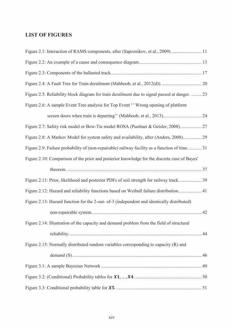
LIST OF FIGURES
Figure 2.1: Interaction of RAMS components, after (Sapoznikov, et al., 2009) .......................... 11
Figure 2.2: An example of a cause and consequence diagram...................................................... 13
Figure 2.3: Components of the ballasted track. ............................................................................. 17
Figure 2.4: A Fault Tree for Train derailment (Mahboob, et al., 2012(d)). .................................. 20
Figure 2.5: Reliability block diagram for train derailment due to signal passed at danger. ......... 23
Figure 2.6: A sample Event Tree analysis for Top Event ‘’ Wrong opening of platform
screen doors when train is departing’’ (Mahboob, et al., 2013). ................................ 24
Figure 2.7: Safety risk model or Bow-Tie model ROSA (Puettner & Geisler, 2008). ................. 27
Figure 2.8: A Markov Model for system safety and availability, after (Anders, 2008). ............... 29
Figure 2.9: Failure probability of (non-repairable) railway facility as a function of time. ........... 31
Figure 2.10: Comparison of the prior and posterior knowledge for the discrete case of Bayes'
theorem. ................................................................................................................... 37
Figure 2.11: Prior, likelihood and posterior PDFs of soil strength for railway track.................... 39
Figure 2.12: Hazard and reliability functions based on Weibull failure distribution. ................... 41
Figure 2.13: Hazard function for the 2-out- of-3 (independent and identically distributed)
non-repairable system. ............................................................................................. 42
Figure 2.14: Illustration of the capacity and demand problem from the field of structural
reliability. ................................................................................................................. 44
Figure 2.15: Normally distributed random variables corresponding to capacity (R) and
demand (S). .............................................................................................................. 46
Figure 3.1: A sample Bayesian Network ...................................................................................... 49
Figure 3.2: (Conditional) Probability tables for . ......................................................... 50
Figure 3.3: Conditional probability table for . ......................................................................... 51
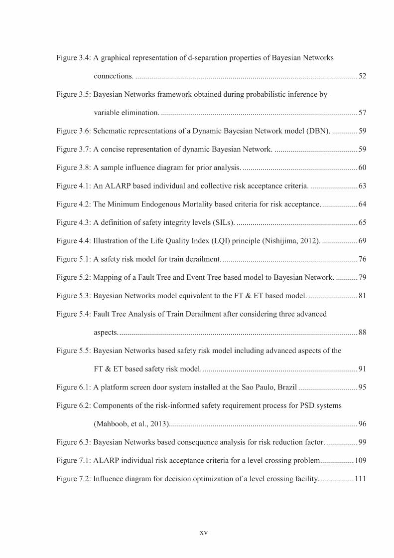
xv
Figure 3.4: A graphical representation of d-separation properties of Bayesian Networks
connections. ................................................................................................................ 52
Figure 3.5: Bayesian Networks framework obtained during probabilistic inference by
variable elimination. ................................................................................................... 57
Figure 3.6: Schematic representations of a Dynamic Bayesian Network model (DBN). ............. 59
Figure 3.7: A concise representation of dynamic Bayesian Network. .......................................... 59
Figure 3.8: A sample influence diagram for prior analysis. .......................................................... 60
Figure 4.1: An ALARP based individual and collective risk acceptance criteria. ........................ 63
Figure 4.2: The Minimum Endogenous Mortality based criteria for risk acceptance. .................. 64
Figure 4.3: A definition of safety integrity levels (SILs). ............................................................. 65
Figure 4.4: Illustration of the Life Quality Index (LQI) principle (Nishijima, 2012). .................. 69
Figure 5.1: A safety risk model for train derailment. .................................................................... 76
Figure 5.2: Mapping of a Fault Tree and Event Tree based model to Bayesian Network. ........... 79
Figure 5.3: Bayesian Networks model equivalent to the FT & ET based model. ......................... 81
Figure 5.4: Fault Tree Analysis of Train Derailment after considering three advanced
aspects. ........................................................................................................................ 88
Figure 5.5: Bayesian Networks based safety risk model including advanced aspects of the
FT & ET based safety risk model. .............................................................................. 91
Figure 6.1: A platform screen door system installed at the Sao Paulo, Brazil .............................. 95
Figure 6.2: Components of the risk-informed safety requirement process for PSD systems
(Mahboob, et al., 2013)............................................................................................... 96
Figure 6.3: Bayesian Networks based consequence analysis for risk reduction factor. ................ 99
Figure 7.1: ALARP individual risk acceptance criteria for a level crossing problem................. 109
Figure 7.2: Influence diagram for decision optimization of a level crossing facility. ................. 111
xvi
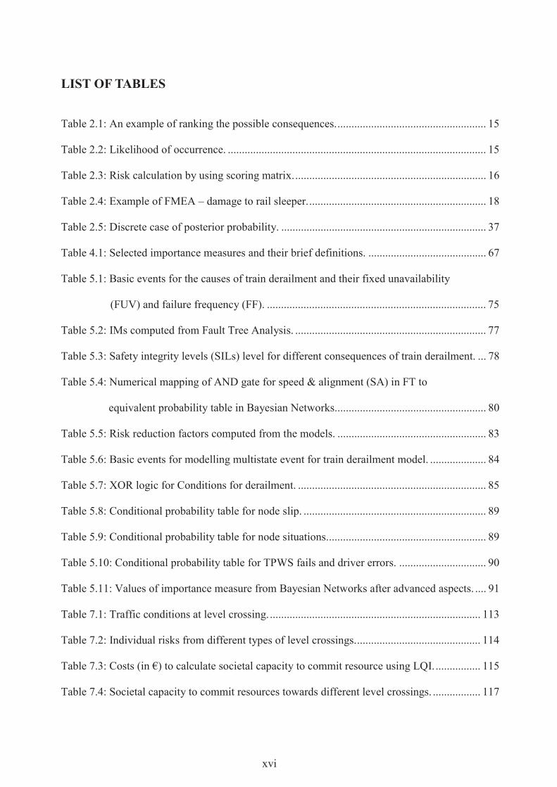
LIST OF TABLES
Table 2.1: An example of ranking the possible consequences. ..................................................... 15
Table 2.2: Likelihood of occurrence. ............................................................................................ 15
Table 2.3: Risk calculation by using scoring matrix. .................................................................... 16
Table 2.4: Example of FMEA – damage to rail sleeper. ............................................................... 18
Table 2.5: Discrete case of posterior probability. ......................................................................... 37
Table 4.1: Selected importance measures and their brief definitions. .......................................... 67
Table 5.1: Basic events for the causes of train derailment and their fixed unavailability
(FUV) and failure frequency (FF). .............................................................................. 75
Table 5.2: IMs computed from Fault Tree Analysis. .................................................................... 77
Table 5.3: Safety integrity levels (SILs) level for different consequences of train derailment. ... 78
Table 5.4: Numerical mapping of AND gate for speed & alignment (SA) in FT to
equivalent probability table in Bayesian Networks...................................................... 80
Table 5.5: Risk reduction factors computed from the models. ..................................................... 83
Table 5.6: Basic events for modelling multistate event for train derailment model. .................... 84
Table 5.7: XOR logic for Conditions for derailment. ................................................................... 85
Table 5.8: Conditional probability table for node slip. ................................................................. 89
Table 5.9: Conditional probability table for node situations. ........................................................ 89
Table 5.10: Conditional probability table for TPWS fails and driver errors. ............................... 90
Table 5.11: Values of importance measure from Bayesian Networks after advanced aspects. .... 91
Table 7.1: Traffic conditions at level crossing. ........................................................................... 113
Table 7.2: Individual risks from different types of level crossings. ............................................ 114
Table 7.3: Costs (in €) to calculate societal capacity to commit resource using LQI. ................ 115
Table 7.4: Societal capacity to commit resources towards different level crossings. ................. 117

xvii
Table 7.5: LQI based costs for different LCs when fatalities are observed. ............................... 117
Table 7.6: Expected utilities (€ per year) of different safety measures for LC. .......................... 118

1
CHAPTER 1: INTRODUCTION
1.1 Need to model and quantify the causes and consequences of hazards on rail-
ways
Rail transportation is an important mode of transport throughout the world. Each day, it
transports millions of passengers and goods from one point to another. For instance, Germa-
ny has the highest number of train-kilometres in Europe ( million of train-kilometres
in 2011) and the railway system serves as the backbone of the country’s land transportation.
The German railway has the highest passenger volume in the EU ( million of pas-
senger-kilometres in 2011) and has had increasing trends over the past three years. Proba-
bly, one of the reasons for the high and increasing passenger-volume on German (and many
other) world railways is that the fatality risks for railway passengers are among the lowest in
land transportation. For instance, one most recently available study in the EU confirms that
railway passengers have lower travelling risks ( fatalities per billion passenger-
kilometres) in comparison to other means of land transportation such as buses ( fatali-
ties per billion passenger-kilometres), cars ( fatalities per billion passenger-
kilometres) and motor-cycles ( fatalities per billion passenger-kilometres) (EU,
2012). Although the safety performance of railways in EU member states is high, serious
accidents continue to occur. For example, a fatal train accident occurred on 24 July, 2013
near to Santiago de Compostela due to high train speed on a curve causing 80 fatalities and
dozens of serious injuries (Spiegel, 2013). Each year, a number of lives are lost due to rail-
way accidents. A recent report published by the European Railway Agency (ERA) indicates
that every year there are approximately 2,400 accidents in EU leading to approximately
1,200 fatalities. Additionally, there are more than 1,000 serious injuries as a result of these
accidents (ERA, 2013). The economic burden of the fatalities and serious injuries was val-
ued at more than 2.5 billion in 2011.
A Bayesian Network Methodology for Railway Risk, Safety and Decision Support
2
The safety and reliability of railway operation and their passengers depend on the reliability
and safety of railway personnel, sub-systems and different technical components. A number
of accidents will occur if the personnel, sub-systems and or components fail to act and work
safely. For instance, a study grouped railways accidents into three categories; rolling stock
(47%), rail and track (39%) and insufficient information (14%) (Holmgren, 2005). The
same study further identified that the rail and track related accidents are mainly caused by
maintenance (30%), railway operation (30%), sabotage (27%) and unknown causes (13%).
Poor maintenance, for instance, mainly leads to mechanical failures. Some mechanical fail-
ures, such as wheel defects, traction motor defects, and control system problems, were re-
ported to be the main causes for delays in commuter service in North American cities
(Nelson & O'Neil, 2000). In addition, the railway systems are subject to a variety of natural
hazards. Through improved risk, safety and reliability modelling techniques, it is possible to
improve the quantification and evaluation of the failure causes and their consequences for
railways.
1.2 State-of-the art techniques in the railway
A number of technical systems and solutions have been introduced to reduce failures and for
safer operation of railways (Maschek, 2012). Methods exist to analyse the failures and their
consequences on the technical systems and solutions (Ericson, 2005). For example, Fault
Tree Analysis (FTA) and Event Tree Analysis (ETA) are common techniques used for logi-
cal representation of a railway system for the purpose of risk and reliability analysis (Chen,
et al., 2007; Braband, et al., 2006; Dhillon, 2007; Bearfield & Marsh, 2005). FTA is based
on top-down logic, starting from the hazard, also called the Top Event (TE), and looking
downwards at all possible combinations of causes of that hazard. ETA models the scenarios
following the hazard and leading to different consequences such as property losses and fa-
talities. Very often, FTA and ETA are combined in one model, also called a bow-tie, which
analyses the causes and the consequences of an accident (Khakzad, et al., 2013). In the rail-
way industry, a combination of the two methods has been used to compute Individual Risk
of Fatality (IRF) and safety integrity requirements for a technical system (Braband, et al.,
2006). In general, both FTA and ETA are based on assumptions which simplify the compu-
Introduction
3
tations, such as independent failures or logically deterministic combinations of causes. It has
been proven that the railway system is rather complex, involving multi-dependencies be-
tween system variables and uncertainties about these dependencies. For example, high train
speed is a common cause of failure; slip and failure of brake applications are disjoint events;
failure dependency exists between the train protection and warning system and driver errors;
driver errors are time dependent and there is functional uncertainty for derailment condi-
tions. Failing to incorporate these complex aspects leads to wrong estimations of the risks
and reliability, and, consequently, to wrong management decisions. Modelling and quantifi-
cation of the railway risk and reliability problems that involve dependencies and uncertain-
ties as mentioned above are complex tasks and require the application of an appropriate tool.
FTA has limitations in modelling complex systems (Khakzad, et al., 2011; Xing & Amari,
2008). In most cases, the FTA structure increases exponentially, becoming non-intuitive and
computationally demanding with an increase in, for example, common cause failures, dis-
joint events and multistate events (Mahboob, et al., 2012(c)). These limitations make the
application of classical methods for the analysis of railway systems difficult.
Importance measures (IMs) can be used to identify and then rank the system components
with respect to their significance towards risk and reliability. IMs can help system designers
in identifying the components that should be improved, assist maintenance engineers to im-
prove maintenance plans for the more critical components and facilitate decision making on
the utilization of engineering budgets for human safety. A number of IMs exist that can be
used for different identifications and rankings (Birnbaum, 1969; Rausand & Hoyland, 2004;
Borgonovo & Apostolakis, 2001). For instance, Risk Achievement Worth (RAW) identifies
the increase in the system risks if a particular component failure in the system has occurred.
The Fussell-Vesely (FV) value gives the fractional contribution of a component failure to-
wards the system failure. An increase in the occurrence probability of the component failure
will lead to an increase in the FV value. For the application of IMs to different industries we
refer to (Borgonovo, et al., 2003; Prescott & Andrews, 2010; Mahboob, et al., 2012(b)).
ALARP is widely accepted as ‘’best practice’’ into the railway industry (Braband, et al.,
2006; Beugin, et al., 2007). ALARP provides several variations in between the two ex-
tremes. In other words, a tolerable region exists between the regions of intolerable and neg-
ligible risks. If the risks fall in the intolerable region then one should adopt safety measures
A Bayesian Network Methodology for Railway Risk, Safety and Decision Support
4
– regardless of cost – to bring the risks into the tolerable region or even below. In the tolera-
ble region, risk reduction is desirable and is undertaken only if some benefit is obtained. The
risk must be made as low as reasonably practicable in the tolerable region (Melchers, 2001).
MEM (Minimum Endogenous Mortality) and MGS (Mindestens Gleiche Sicherheit) are al-
so well applied risk acceptance criteria in the field of railways, see Chapter 4 for their brief
introduction.
In many cases the problem of risk acceptance turns into an economic decision problem
when the risks are in the so-called ALARP region and the objective is to further reduce the
risks. In this situation, socio-economic considerations, such as benefit-cost analysis (BCA)
have been utilized for railway risk management. In BCA, the profitability of a safety tech-
nology is calculated by quantifying the willingness-to-pay (WTP) (from the society point of
view). WTP is the amount that people are willing to pay to save a human life. The BCA and
the WTP approaches are well applied and usually accepted methods for valuing the preven-
tion of fatalities (Evans, 2013; TD, 2000; Aoun, et al., 2012; RSSB, 2006; Evans, 2005). Of
course, one can disregard BCA or WTP in the adoption of safety technology if the aim is to
prevent and mitigate train collisions and derailments. The usual reason for the disregard is
that a higher safety technology is needed than would be calculated by BCA. However, some
areas of safety improvement such as upgrades or replacements of level crossings (LCs) are
good subjects for BCA (Evans, 2013). The BCA takes into account the same parameters for
the comparison of profitability of different safety technologies. Identification of such pa-
rameters for different socio-economic and geographical conditions and the assignment of
monetary values (to benefits and costs) of the identified parameters always have complica-
tions. The BCA and WTP approaches become difficult to use if the parameters of the deci-
sion problem are not completely known.
1.3 Goals and scope of work
The goal of this research work is to investigate the application of Bayesian Networks as a
decision support framework for railway risk and safety. This thesis explores various im-
portant aspects of the modelling and analysis of railway risks and how an improvement can
be achieved in the risk-based decision making process. The work mainly focuses on the de-
Introduction
5
velopment of a framework that can handle complexities and uncertainties in modern rail-
ways. It investigates how the economic considerations can be incorporated within the mod-
els so that the decision making on railway engineering budgets can further be facilitated.
Visualization of the framework (in understanding the system variables, decision alternatives
and risk acceptance criteria) is often required to facilitate the decision making process;
therefore, compact and concise visualization of the model is necessary to provide a decision
aid for the decision maker.
In view of the above, it has been determined that Bayesian Networks can provide a suitable
tool to meet the modelling, analysis and decision support requirements above. Bayesian
Networks are directed acyclic probabilistic graphical models that handle the joint distribu-
tion of random variables in a compact and flexible way. The following characteristics of
Bayesian Networks make them suitable for railway risk, safety and decision support:
1) Bayesian Networks can handle multiple hazards and a number of dependencies and
uncertainties among (the random variables of) different hazards and within a hazard.
The dependencies can arise due to common cause, multistate and disjoint events in
the hazard models.
2) Repetition of the random variables is not required for dependencies in Bayesian
Networks. Thus, Bayesian Networks offer a concise and intuitive visualization of a
framework which makes it useful for discussions among the designers, manufactur-
ers, operators and decision makers who may not be expert in probabilistic risk as-
sessment.
3) Bayesian Networks are able to update the hazard model in two ways. Top-down up-
dating is obtained when the information propagates from the top, that is, from the
hazard down to the basic causes of the hazards. In bottom-up updating, information
propagates from the basic causes towards the hazard. For instance, by exploiting the
use of the updating characteristics of the Bayesian Networks, one can account, at the
same time, not only for the components that have failed, but also for those that are
working.
A Bayesian Network Methodology for Railway Risk, Safety and Decision Support
6
4) Influence diagrams (IDs) are extensions of Bayesian Networks. Problems of proba-
bilistic inference and decision making can be combined and optimized in IDs. They
offers a decision tool for ranking alternatives based on expected utility.
In this thesis, we propose a Bayesian Network based methodology for performing railway
risk and safety assessment. We show how the dependencies, uncertainties, expert
knowledge and economics related aspects of a complex railway system can be tackled using
Bayesian Networks for risk-based decision making.
1.4 Existing work
There are few applications of Bayesian Networks to railways. Importantly, these applica-
tions do not belong to the development of the IDs based decision framework for railway
risks. (Marsh & Bearfield, 2007) use Bayesian Network for the representation of a parame-
terized FTA for SPAD1; (Oukhellou, et al., 2008) developed a Bayesian Network model for
identifying and classifying rail defects based on sensor data; (Lu, et al., 2011) proposed a
Bayesian Network approach to model the causal relationships among risk factors for sub-
way systems; (Vatn & Svee, 2002) applied an influence diagram for decision making on the
ultrasonic inspection of rails; (Flammini, et al., 2009) applied Bayesian Networks for quan-
titative security risk assessment and management for railway transportation infrastructures.
Risk models for railway accidents using IDs have not been studied extensively. No studies
exist on how to model and analyse risks in complex railways – characterized by a number of
advanced aspects, explained in Chapter 5 – using Bayesian Networks. The computation of
the IMs for complex system’s components using Bayesian Networks has not been discussed
so far, especially, for railways. Therefore, the work in this thesis is novel with respect to the
computation of IMs and the modelling and analysis of advanced aspects of risk models for
complex railways using Bayesian Network and IDs based decision support for railway risks
and safety cases. The LQI is a relatively new utility-based risk acceptance criterion and its
application to the railway industry, to justify the investment in railway risks, is novel. How-
1 SPAD (signal passed at danger) in railways occurs when a train passes a stop signal without permission to do so.
Introduction
7
ever, the LQI is a well applied and accepted risk acceptance criterion from the field of struc-
tural safety. To the knowledge of the author, IDs based applied tools for railway risk man-
agement do not exist. However, some studies have suggested and developed such tools for
fields other than railways (Hanea, 2009(a); Straub, 2005; Faber, et al., 2012; Bensi, et al.,
2011).
1.5 Outline of the thesis
This thesis proposes a Bayesian Network methodology for risk assessment and decision
support in reference to railways. The thesis is organized in 8 chapters. The motivation, state-
of-the-art work and goals and scope of the research work are presented in the Introduction.
Chapter 2 provides an introduction to the methods for safety and risk analysis for railways.
This chapter deals with the basic concepts and definitions of risk and safety. A review of the
many existing methods and approaches, which are well applied to engineering risk prob-
lems, including railways engineering, is presented. A brief description is given for the sim-
plest methods such as risk matrix, model based methods such as fault tree and numerical
methods such as hazard function and Monte Carlo simulation. Each method is described
with the help of a suitable example from the railways.
Chapter 3 reviews Bayesian Networks. Here, sufficient introduction to Bayesian Networks
is provided so that methods and models presented in the following chapters can be better
understood. It provides a brief introduction to terminology such as conditional independ-
ence, joint distribution and Markov blanket in a Bayesian Network. Construction of a
Bayesian Network and probabilistic inference methods, such as inference by enumeration
and variable elimination, are described with the help of examples. A brief introduction of
IDs is presented.
Chapter 4 describes risk acceptance criteria and determination of safety targets in railways.
The classical way of representing risks arising from a railway system is the individual risk
which is expressed in terms of an annual fatality rate for a person exposed to the given situa-
tion at a given point in time. Individual risk acceptance criteria, based on the ALARP, MEM
and MGS approaches, are explained. The LQI is also briefly explained in Chapter 4. The
A Bayesian Network Methodology for Railway Risk, Safety and Decision Support
8
LQI treats the risk acceptance criterion as an economic decision problem in an uncertain
environment by establishing a relation between the resources utilized in improving the safe-
ty of a system and fatalities that can be avoided by the resources. It offers a rational way of
finding acceptable decisions on engineering systems involving risks to human life.
The exact quantification of systematic errors (mainly caused by humans) is not possible;
however, random failures can be quantified. The idea behind the safety integrity level (SIL)
concept is to create a balance between the measures for preventing systematic errors and
random failures.
This chapter explains the concept of IMs. The components with higher importance with re-
spect to risk are treated carefully in the design, maintenance and operation of an engineering
system. The definitions of selected IMs, which are used to identify and rank the important
components in a system, are given here.
Chapter 5 provides an example application, which demonstrates the complexity of risk
models in railways. The example of train derailment is used to show how Bayesian Net-
works can be used to model dependencies, uncertainties and expert knowledge for a railway
risk problem. This chapter focuses on the modelling of advanced aspects of fault trees using
Bayesian Networks. A fault tree and event tree based safety risk model is translated into a
Bayesian Network, consequences of the railway hazard ‘’train derailment’’ are quantified
and the IMs for the events leading to the hazard are computed.
Chapter 6 presents a real-world application of Bayesian Networks. Mega cities across the
world will continue to grow during the 21st century. Urban rail transit systems (URTSs) in
such mega cities are subject to different hazards, which can lead to life safety risks. Bayesi-
an Networks are applied to quantify the risk-based safety integrity requirements for a PSD
(Platform Screen Door) system in a typical mega city. The steps in the risk-informed safety
requirement process are explained for the PSD system. A number of hazardous situations
related to a PSD system, so-called hazardous situations, are identified. A preliminary cause
and consequence analysis is carried out to scrutinize the most important hazardous situa-
tions. The consequences of these most relevant hazardous events are modelled for specific
operational conditions. The identified consequences are quantified and then compared to
Introduction
9
risk acceptance criteria for assessment. The risk-informed SIL requirements are determined
for the PSD system.
Chapter 7 focuses on the justification of the investment in human safety in reference to a
railway LC. We apply IDs to the assessment of life safety risks in a railway LC. Individual
risk of fatality at a particular LC is determined for different safety technology solutions. The
ALARP criteria in combination with the LQI are used to identify an optimal and socially
acceptable safety solution for the LC. The LQI-based utilities are used in the IDs to opti-
mize the decision problems.
Chapter 8 concludes the thesis by providing a summary, important contributions and sug-
gesting future research work in this area.
CHAPTER 2: METHODS FOR SAFETY AND RISK ANALYSIS
2.1 Introduction
The railway system related standard EN 50126 (and CENELEC-Standard regarding func-
tional safety 2006) introduces the RAMS (Reliability, Availability, Maintainability, and
Safety) concept (CENELEC, 2012; Braband, et al., 2006). This standard provides RAMS
specifications and requires the railway suppliers and operators to implement a RAMS man-
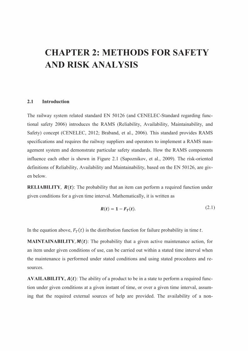
agement system and demonstrate particular safety standards. How the RAMS components
influence each other is shown in Figure 2.1 (Sapoznikov, et al., 2009). The risk-oriented
definitions of Reliability, Availability and Maintainability, based on the EN 50126, are giv-
en below.
RELIABILITY : The probability that an item can perform a required function under
given conditions for a given time interval. Mathematically, it is written as
(2.1)
In the equation above, is the distribution function for failure probability in time .
MAINTAINABILITY : The probability that a given active maintenance action, for
an item under given conditions of use, can be carried out within a stated time interval when
the maintenance is performed under stated conditions and using stated procedures and re-
sources.
AVAILABILITY, : The ability of a product to be in a state to perform a required func-
tion under given conditions at a given instant of time, or over a given time interval, assum-
ing that the required external sources of help are provided. The availability of a non-
Methods for safety and risk analysis
11
repairable system is equivalent to the system reliability. In the case of a repairable system
the availability becomes,
(2.2)
In the equation above, is the distribution function for maintenance rate in time In
general, safety concept relates to the control of recognized hazards in order to achieve a
‘’acceptable level of risk’’. However, the term SAFETY, according to the CENELEC
standards, is freedom from unacceptable risks, danger and injury from a technical failure in
railways. The RISK of a hazard is defined as the product of the probability (or likeli-
hood) of a hazard and the consequences (such as fatality and costs) of a hazard :
(2.3)
The mathematical definition of risk is expected adverse consequences (Straub, 2011; Zio,
2007). The hazard is a physical situation, which has a potential for harm.
Figure 2.1: Interaction of RAMS components, after (Sapoznikov, et al., 2009)
A Bayesian Network Methodology for Railway Risk, Safety and Decision Support
12
Safety management in railway engineering systems is based on the combination of reactive
approaches (like learning from accidents and mistakes) and proactive approaches (like risk
and safety case analysis). This work focuses on the proactive approaches; therefore, mainly
risk and safety case analysis will be dealt with here. Risk assessment is the process of identi-
fying and analysing potential losses from a given failure in engineering systems such as
railways. The risk assessment uses a combination of known information about the hazardous
situation, knowledge about the underlying phenomenon or process and judgement about the
information that is not certain or well understood. All unwanted situations – so-called haz-
ards – are postulated and their consequences are modelled (Ericson, 2005; Mohaghegh, et
al., 2009; Mahboob, et al., 2012(b); Podofillini, et al., 2006). The safety integrity require-
ments are then determined for the system, which is under different risks. Methods for risk
analysis can be classified into three main categories (Ericson, 2005; Aven, 2008).
2.1.1 Simplified risk analysis
This is an informal procedure based on qualitative approaches. It establishes the risk picture
using brainstorming sessions and group discussions. Group members are the expert in the
field in which risk analysis is being carried out. The risk might be presented on a coarse
scale, for example, low, moderate or high, making no use of formalized risk analysis meth-
ods.
2.1.2 Standard risk analysis
This is a more formalized procedure and includes both qualitative and quantitative ap-
proaches. In this analysis, more recognized methods such as Preliminary Hazard Analysis
(PHA), Hazard and Operability (HAZOP) studies, Failure Modes and Effect Analysis
(FMEA) and coarse risk analysis are utilized.
2.1.3 Model-based risk analysis
This is primarily a quantitative approach. Information obtained from the above two catego-
ries may be used in the development of a representation of the overall system in terms of
logic diagrams, for example, Fault Tree, Reliability Block Diagram and Bayesian Networks.
Methods for safety and risk analysis
13
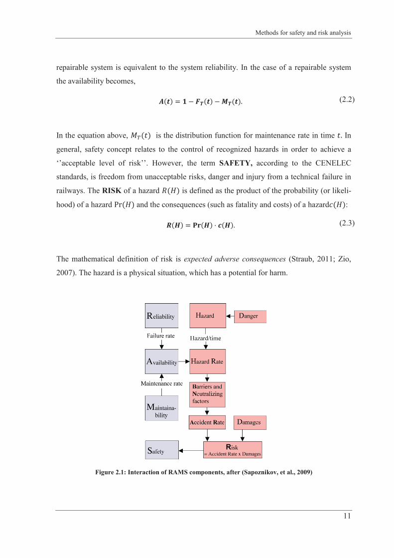
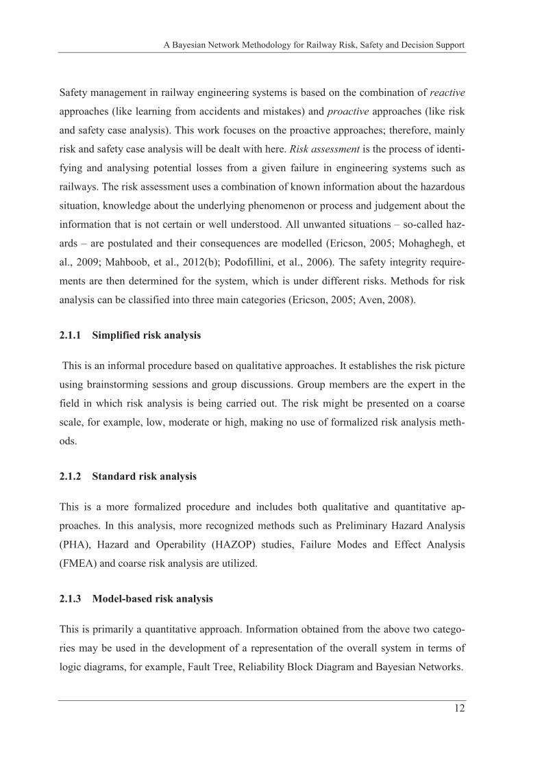
Figure 2.2: An example of a cause and consequence diagram.
The purpose of risk and safety assessment is to identify, determine and assess the risks pre-
sent in a system. Systems can be engineering, social, natural and others. One way of deter-
mining and assessing risk is to utilize a cause and consequence diagram. For instance, Fig-
ure 2.2 shows a classical example of cause and consequence analysis where the hazard, also
called the TE is located in the centre of the figure. This figure portrays the Fault Symptom
approach where the fault represents the cause (lower part in Figure 2.2) and the symptom
the consequence (upper part in Figure 2.2). There are barriers and neutralizing factors,
which may prevent hazard occurrence and its propagation. There can be a large number of
faults and symptoms in a cause and consequence diagram.
A Bayesian Network Methodology for Railway Risk, Safety and Decision Support
14
The causes of a TE can be failure in system components, human error and environmental
effects. The consequences of a TE can be life safety risks to an individual person or society,
environmental damages, structural damages or loss of production and services. Identifica-
tion of the TE is an important task. Risk analysis has to identify the TEs and to develop the
cause and consequence picture. How this is done depends on which method is adopted and
how the results are utilized. However, the intent is always the same: to describe the risks in
the system. Some methods used for railway risk and safety are briefly explained in the fol-
lowing.
2.2 Risk Matrix
This is also referred to as preliminary risk analysis. The risk matrix approach is mainly
semi-quantitative. It becomes easy to use and understand, provided that the following main
drawbacks of the risk matrix are resolved (Braband, 2010):
calibration for particular application is required;
the risk results are only valid for the system to which the risk matrices are ap-
plied; and
the parameters (such as frequency and likelihood) are based on subjective defini-
tions, which may lead to understanding complexities.
How analysis using risk matrix is performed is shown in the following three steps.
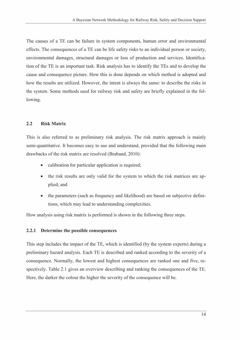
2.2.1 Determine the possible consequences
This step includes the impact of the TE, which is identified (by the system experts) during a
preliminary hazard analysis. Each TE is described and ranked according to the severity of a
consequence. Normally, the lowest and highest consequences are ranked one and five, re-
spectively. Table 2.1 gives an overview describing and ranking the consequences of the TE.
Here, the darker the colour the higher the severity of the consequence will be.
Methods for safety and risk analysis
15
Table 2.1: An example of ranking the possible consequences.
Description Of event
1 2 3 4 5 Insignificant Minor Moderate Major Catastrophe
Injury Minor injury without first aid
Minor inju-ry with first aid
Major injury, hospitalized
Long term inca-pacity, disability
Death, perma-nent incapacity
Service loss Service suspen-sion for one hour
Loss of ser-vice for 08 hours
Loss of service for one day
Loss of service for one week
Permanent loss of facility
Staffing and competence
Temporary loss in service (< 1 day)
Reduces service quality
Minor er-rors/defects
Serious er-rors/defects
Critical er-rors/defects
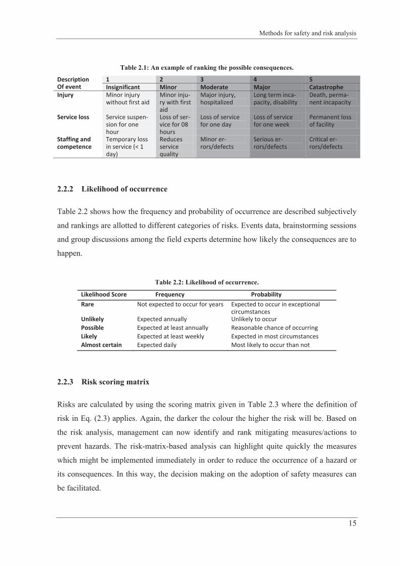
2.2.2 Likelihood of occurrence
Table 2.2 shows how the frequency and probability of occurrence are described subjectively
and rankings are allotted to different categories of risks. Events data, brainstorming sessions
and group discussions among the field experts determine how likely the consequences are to
happen.
Table 2.2: Likelihood of occurrence.
Likelihood Score Frequency Probability Rare Not expected to occur for years Expected to occur in exceptional
circumstances Unlikely Expected annually Unlikely to occur Possible Expected at least annually Reasonable chance of occurring Likely Expected at least weekly Expected in most circumstances Almost certain Expected daily Most likely to occur than not
2.2.3 Risk scoring matrix
Risks are calculated by using the scoring matrix given in Table 2.3 where the definition of
risk in Eq. (2.3) applies. Again, the darker the colour the higher the risk will be. Based on
the risk analysis, management can now identify and rank mitigating measures/actions to
prevent hazards. The risk-matrix-based analysis can highlight quite quickly the measures
which might be implemented immediately in order to reduce the occurrence of a hazard or
its consequences. In this way, the decision making on the adoption of safety measures can
be facilitated.
A Bayesian Network Methodology for Railway Risk, Safety and Decision Support
16
Table 2.3: Risk calculation by using scoring matrix.
Likelihood score
Consequences 1 Insignificant
2 Minor
3 Moderate
4 Major
5 Catastrophe
1. Rare 1 2 3 4 5 2. Unlikely 2 4 6 8 10 3. Possible 3 6 9 12 15 4. Likely 4 8 12 16 20 5. Almost certain 5 10 15 20 25 1-3 is Low; 4-6 is Moderate; 8-12 is High; 15-25 is Extreme
2.3 Failure Modes & Effect Analysis – FMEA
FMEA is a bottom-up approach in analysing the effects of potential failure modes in an en-
gineering system (Recht, 1966). It is a relatively simple method to determine possible fail-
ures and to predict the failure effects on the system. Investigation is carried out as to what
happens if a particular component fails. The method represents a systematic analysis of the
components of the system to identify all significant failure modes and to see how important
they are for the system’s safety and performance. Only one component is considered at a
time, and it is assumed that other components are working at the same time. In this way,
FMEA is not suitable for determining critical combinations of component failures.
Failure Modes, Effects and Criticality Analysis (FMECA) is an extension of FMEA. If criti-
cality ranking for various failures in FMEA is added, we obtain a complete form of FMECA
(Stewart & Melchers, 1997). The criticality is a function of the failure effect and the fre-
quency or probability. The difference between an FMEA and an FMECA is not distinct, and
sometime experts dealing with risk analysis do not distinguish between these two types of
analysis (Aven, 2008). They also use criticality ranking as a part of FMEA. In order to en-
sure systematic study of the technical system, a specific FMECA form (see Table 2.4) is
used for this purpose.
Methods for safety and risk analysis
17
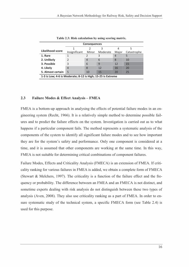
2.3.1 Example application of FMEA
A number of factors must be considered carefully before the implementation of an FMEA.
For example, examination of each possible failure mode, costs/benefits of FMEA and its
implementation, engineers’ approval and decision making on the basis of risk criticality are
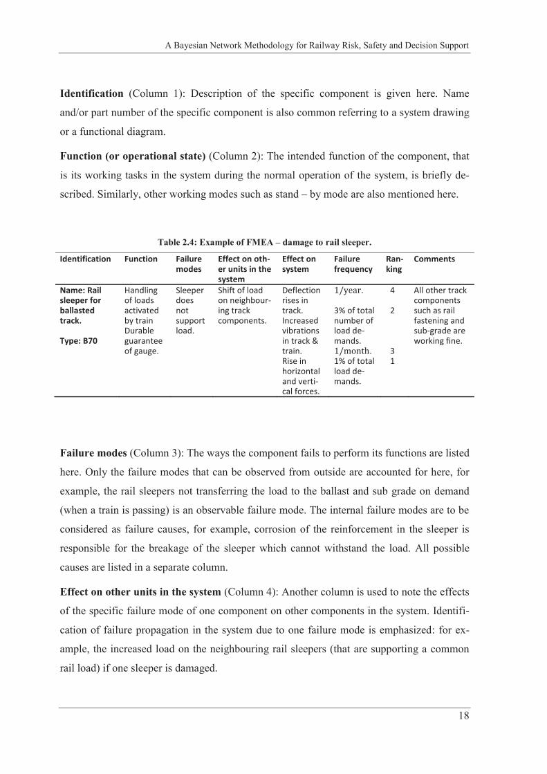
important (Dhillon, 2011). In the following example of a rail sleeper, we also use the term
FMEA when the analysis includes a ranking of criticality. A schematic representation of the
ballasted railway track is shown in Figure 2.3.
Figure 2.3: Components of the ballasted track.
The main function of the rail sleeper is to provide a durable guarantee of rail gauge, rail in-
clination and handling for all types of loads activated by vehicles. It also provides resistance
during the thermal changes in the rail and transfers the load into the ballast bed and sub-
structure (Ford, 2001). Rail sleepers can create hazards when they do not perform their
function of supporting the rail and train load. An FMEA for the specific failure mode, load
not supported by the sleeper, is presented in Table 2.4 and the general descriptions of the
columns are explained below.
A Bayesian Network Methodology for Railway Risk, Safety and Decision Support
18
Identification (Column 1): Description of the specific component is given here. Name
and/or part number of the specific component is also common referring to a system drawing
or a functional diagram.
Function (or operational state) (Column 2): The intended function of the component, that
is its working tasks in the system during the normal operation of the system, is briefly de-
scribed. Similarly, other working modes such as stand – by mode are also mentioned here.
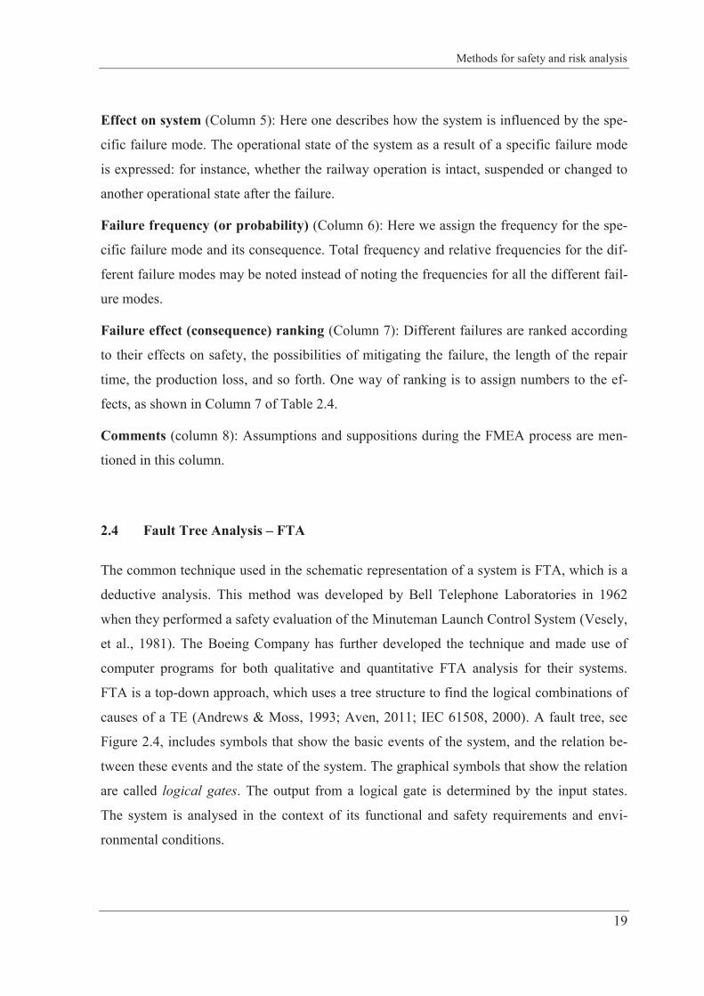
Table 2.4: Example of FMEA – damage to rail sleeper.
Identification Function Failure modes
Effect on oth-er units in the system
Effect on system
Failure frequency
Ran-king
Comments
Name: Rail sleeper for ballasted track. Type: B70
Handling of loads activated by train Durable guarantee of gauge.
Sleeper does not support load.
Shift of load on neighbour-ing track components.
Deflection rises in track. Increased vibrations in track & train. Rise in horizontal and verti-cal forces.
. 3% of total number of load de-mands.
. 1% of total load de-mands.
4 2 3 1
All other track components such as rail fastening and sub-grade are working fine.
Failure modes (Column 3): The ways the component fails to perform its functions are listed
here. Only the failure modes that can be observed from outside are accounted for here, for
example, the rail sleepers not transferring the load to the ballast and sub grade on demand
(when a train is passing) is an observable failure mode. The internal failure modes are to be
considered as failure causes, for example, corrosion of the reinforcement in the sleeper is
responsible for the breakage of the sleeper which cannot withstand the load. All possible
causes are listed in a separate column.
Effect on other units in the system (Column 4): Another column is used to note the effects
of the specific failure mode of one component on other components in the system. Identifi-
cation of failure propagation in the system due to one failure mode is emphasized: for ex-
ample, the increased load on the neighbouring rail sleepers (that are supporting a common
rail load) if one sleeper is damaged.
Methods for safety and risk analysis
19
Effect on system (Column 5): Here one describes how the system is influenced by the spe-
cific failure mode. The operational state of the system as a result of a specific failure mode
is expressed: for instance, whether the railway operation is intact, suspended or changed to
another operational state after the failure.
Failure frequency (or probability) (Column 6): Here we assign the frequency for the spe-
cific failure mode and its consequence. Total frequency and relative frequencies for the dif-
ferent failure modes may be noted instead of noting the frequencies for all the different fail-
ure modes.
Failure effect (consequence) ranking (Column 7): Different failures are ranked according
to their effects on safety, the possibilities of mitigating the failure, the length of the repair
time, the production loss, and so forth. One way of ranking is to assign numbers to the ef-
fects, as shown in Column 7 of Table 2.4.
Comments (column 8): Assumptions and suppositions during the FMEA process are men-
tioned in this column.
2.4 Fault Tree Analysis – FTA
The common technique used in the schematic representation of a system is FTA, which is a
deductive analysis. This method was developed by Bell Telephone Laboratories in 1962
when they performed a safety evaluation of the Minuteman Launch Control System (Vesely,
et al., 1981). The Boeing Company has further developed the technique and made use of
computer programs for both qualitative and quantitative FTA analysis for their systems.
FTA is a top-down approach, which uses a tree structure to find the logical combinations of
causes of a TE (Andrews & Moss, 1993; Aven, 2011; IEC 61508, 2000). A fault tree, see
Figure 2.4, includes symbols that show the basic events of the system, and the relation be-
tween these events and the state of the system. The graphical symbols that show the relation
are called logical gates. The output from a logical gate is determined by the input states.
The system is analysed in the context of its functional and safety requirements and envi-
ronmental conditions.
A Bayesian Network Methodology for Railway Risk, Safety and Decision Support
20
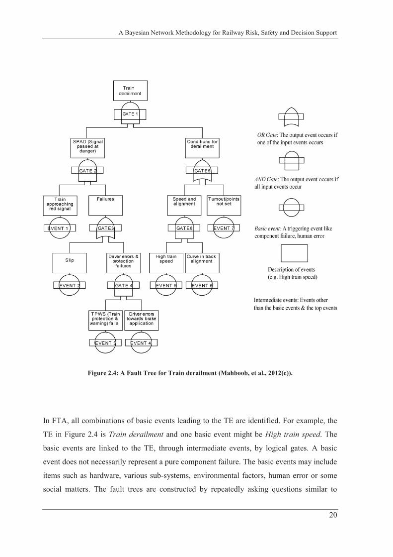
Figure 2.4: A Fault Tree for Train derailment (Mahboob, et al., 2012(c)).
In FTA, all combinations of basic events leading to the TE are identified. For example, the
TE in Figure 2.4 is Train derailment and one basic event might be High train speed. The
basic events are linked to the TE, through intermediate events, by logical gates. A basic
event does not necessarily represent a pure component failure. The basic events may include
items such as hardware, various sub-systems, environmental factors, human error or some
social matters. The fault trees are constructed by repeatedly asking questions similar to
Methods for safety and risk analysis
21
“What can be the causes of the TE?” Further progress in the causal relationship between the
basic and intermediate events is stopped when we have reached the desired level of detail.
Fault trees are dependent on the local conditions of the system; therefore, it is essential to
think locally, and develop the fault tree using a systematic approach.
A standard FTA involves the following steps.
Understand the system design and operation through data, drawings, procedures,
diagrams, and so on.
Define the problem and establish the correct TE (undesired events) for the analy-
sis.
Define the system rules and boundaries. What is included and what cannot be in-
cluded?
Follow the rules, boundaries, and logic (OR, AND,...) to build the FT model.
Generate cut sets and compute probability values for the cut sets.
Identify weak links and safety problems in the design and operation.
Validate the FT model: check if the FT model is correct, complete, and accurate-
ly reflects system design and operation. Modify the FT if necessary during vali-
dation.
Document the entire analysis with supporting data.
A cut set in the FTA is a group of basic events whose combined occurrence can cause the
TE to occur. A cut set will be minimal if it cannot be reduced further and still promises the
occurrence of the TE. Each minimal cut set is viewed as a parallel system of its components
and the overall system state is viewed as a series system of the minimal cut sets. The basic
assumptions of the standard FTA include (1) the events in FTA represent random variables
with binary states (occurring/not occurring) and (2) basic events are statistically independ-
ent. In general, the probability of TE ( ) in the FT is computed as the function of the
minimal cut sets by using the inclusion and exclusion principle in Eq. (2.4).
A Bayesian Network Methodology for Railway Risk, Safety and Decision Support
22
(2.4)
In the equation above, denotes the probability of the occurrence of minimal cut sets
in an FT and is the number of minimal cut sets. For instance, the cut sets in the FT in Fig-
ure 2.4 are . In the
cut set representation above, we denote basic events in the FTA with their first letter, say
for basic event 1. The total number of events in a cut set is called the order of the cut set. At
least terms need to be calculated in order to calculate the . In this way, the solu-
tion becomes computationally demanding when increases. To avoid computational com-
plexities the disjoint sum of the minimal cut sets is also used
(2.5)
In the equation above, .
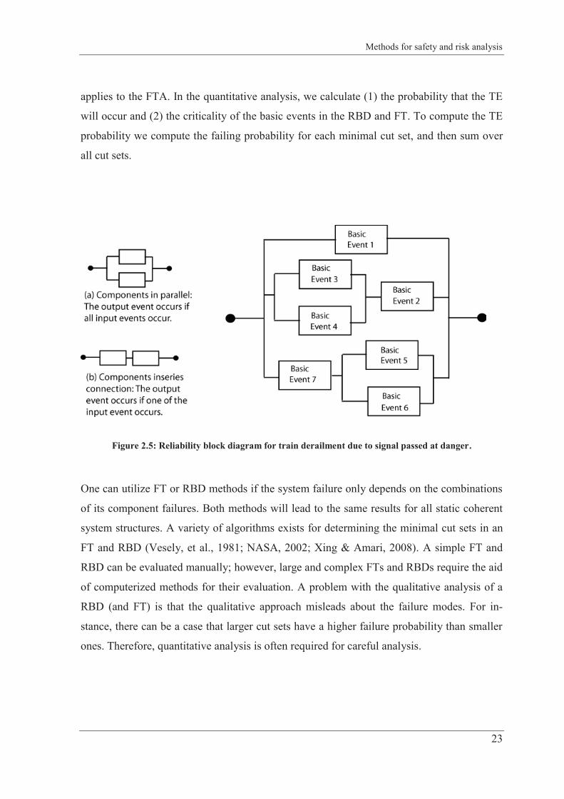
2.5 Reliability Block Diagram – RBD
A fault tree comprising only of AND and OR gates can be represented by an RBD. The
RBD is also a graphical representation showing how component reliability can lead to the
success or failure of a technical system. The graphical framework consists of blocks, which
correspond to the components (or failure events) in the system, connected in series or paral-
lel. The RBD can specify various combinations of components that can lead to a specific
state or performance level of the system. The RBD equivalent to the FT in Figure 2.4 is
shown in Figure 2.5.
It can be seen that the RBD is a combination of parallel and series systems. For a parallel
system, all components must fail for the system to fail. Conversely, in a series system, all
components must function for the successful operation of the system. In other words, the
weakest element in the series system will be the strength of the overall system. The same
Methods for safety and risk analysis
23
applies to the FTA. In the quantitative analysis, we calculate (1) the probability that the TE
will occur and (2) the criticality of the basic events in the RBD and FT. To compute the TE
probability we compute the failing probability for each minimal cut set, and then sum over
all cut sets.
Figure 2.5: Reliability block diagram for train derailment due to signal passed at danger.
One can utilize FT or RBD methods if the system failure only depends on the combinations
of its component failures. Both methods will lead to the same results for all static coherent
system structures. A variety of algorithms exists for determining the minimal cut sets in an
FT and RBD (Vesely, et al., 1981; NASA, 2002; Xing & Amari, 2008). A simple FT and
RBD can be evaluated manually; however, large and complex FTs and RBDs require the aid
of computerized methods for their evaluation. A problem with the qualitative analysis of a
RBD (and FT) is that the qualitative approach misleads about the failure modes. For in-
stance, there can be a case that larger cut sets have a higher failure probability than smaller
ones. Therefore, quantitative analysis is often required for careful analysis.
A Bayesian Network Methodology for Railway Risk, Safety and Decision Support
24
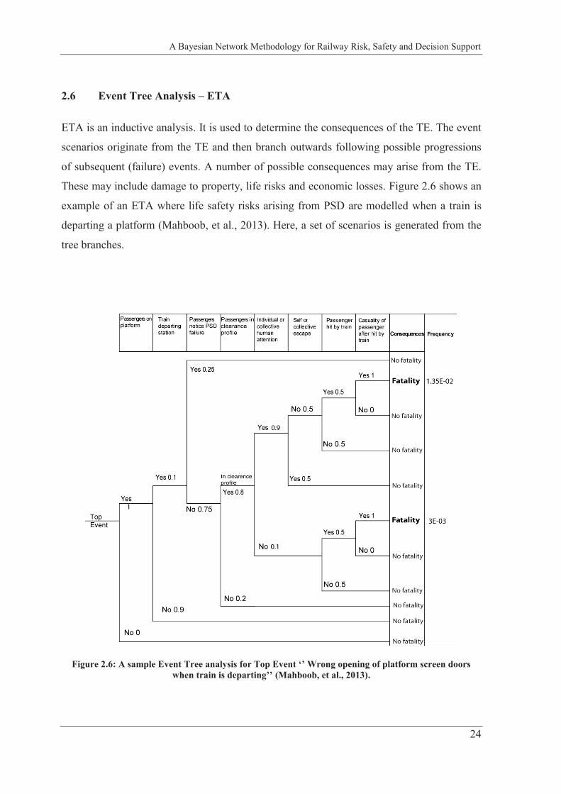
2.6 Event Tree Analysis – ETA
ETA is an inductive analysis. It is used to determine the consequences of the TE. The event
scenarios originate from the TE and then branch outwards following possible progressions
of subsequent (failure) events. A number of possible consequences may arise from the TE.
These may include damage to property, life risks and economic losses. Figure 2.6 shows an
example of an ETA where life safety risks arising from PSD are modelled when a train is
departing a platform (Mahboob, et al., 2013). Here, a set of scenarios is generated from the
tree branches.
Figure 2.6: A sample Event Tree analysis for Top Event ‘’ Wrong opening of platform screen doors when train is departing’’ (Mahboob, et al., 2013).
Methods for safety and risk analysis
25
It is common to pose the branch questions in such a way that the answers to all the branch-
es’ questions are yes or no. In this way, two scenarios will come out, the best at one end and
the worst at the other. Finally, the consequence matrix is drawn, which describes the conse-
quences arising from each terminating event. In Figure 2.6, the consequences are restricted
to the (frequencies of) fatalities. In the quantitative analysis of the ET, frequencies (or prob-
abilities) are linked to the various event scenarios and their consequences. It should be men-
tioned that definitions of the cut sets are also applicable to ETs. The probability of each con-
sequence is computed by multiplying the probability of the initiating event (that is TE in the
FTA) with the probabilities of the events defining each scenario. For example, one of the
probabilities of fatality in Figure 2.6 is calculated by multiplying
2.7 Safety Risk Model – SRM
For systems in which accidents are frequent such as highways the statistical analysis of past
accidents is carried out by estimating quantities such as (e.g. failure rate) and (e.g. arri-
val rate) that are not directly observable. For systems such as railways or aviation, in which
accidents are much less frequent and have more variable outcomes, statistical analysis of the
data is still possible, but the precision of the estimates of the parameters is much lower. For
systems in which accidents are very rare and accident data is so small in number, direct sta-
tistical analysis of accident data is of little help in estimating the risk. In this case risk mod-
els are developed which are specific to the system, and estimate risks by modelling both the
precursor and potential consequences of the hazards. For some systems, the risks are esti-
mated by both of the above methods in a model called SRM or Bow-Tie model. The SRM is
a large scale fault-tree and event-tree based model used to assess risk in engineering sys-
tems. In railways, the SRM was first applied to assess the risk in the mainline railways in
the UK (RS, 2001). The main objective of this SRM was to develop a basic understanding
of the nature and information of the current risks relating to the mainline railways in the
UK. The model consists of 120 hazardous events and over 4000 consequences that collec-
tively determine the mainline railway risks. The base event probabilities are determined
from the historical data of accidents and incidents. In this way, SRM averages the network-
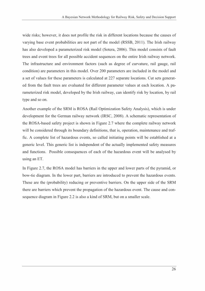
A Bayesian Network Methodology for Railway Risk, Safety and Decision Support
26
wide risks; however, it does not profile the risk in different locations because the causes of
varying base event probabilities are not part of the model (RSSB, 2011). The Irish railway
has also developed a parameterized risk model (Sotera, 2006). This model consists of fault
trees and event trees for all possible accident sequences on the entire Irish railway network.
The infrastructure and environment factors (such as degree of curvature, rail gauge, rail
condition) are parameters in this model. Over 200 parameters are included in the model and
a set of values for these parameters is calculated at 227 separate locations. Cut sets generat-
ed from the fault trees are evaluated for different parameter values at each location. A pa-
rameterized risk model, developed by the Irish railway, can identify risk by location, by rail
type and so on.
Another example of the SRM is ROSA (Rail Optimization Safety Analysis), which is under
development for the German railway network (IRSC, 2008). A schematic representation of
the ROSA-based safety project is shown in Figure 2.7 where the complete railway network
will be considered through its boundary definitions, that is, operation, maintenance and traf-
fic. A complete list of hazardous events, so called initiating points will be established at a
generic level. This generic list is independent of the actually implemented safety measures
and functions. Possible consequences of each of the hazardous event will be analysed by
using an ET.
In Figure 2.7, the ROSA model has barriers in the upper and lower parts of the pyramid, or
bow-tie diagram. In the lower part, barriers are introduced to prevent the hazardous events.
These are the (probability) reducing or preventive barriers. On the upper side of the SRM
there are barriers which prevent the propagation of the hazardous event. The cause and con-
sequence diagram in Figure 2.2 is also a kind of SRM, but on a smaller scale.
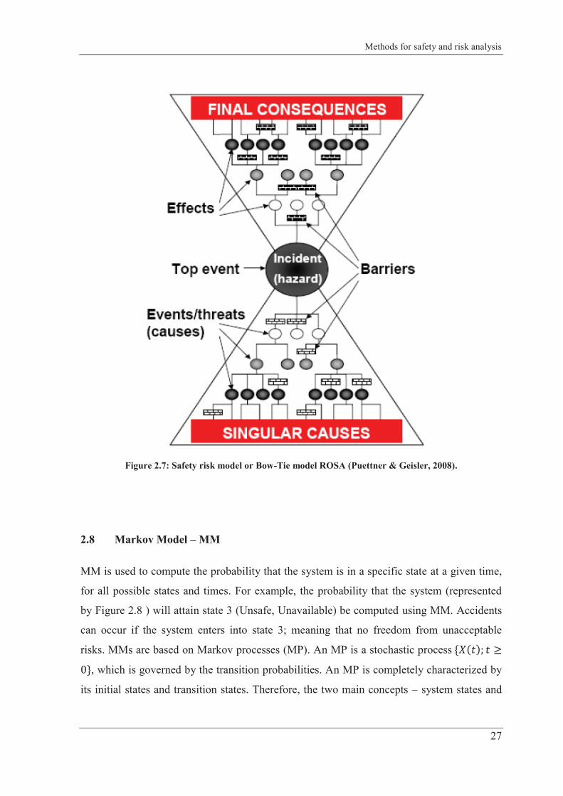
Methods for safety and risk analysis
27
Figure 2.7: Safety risk model or Bow-Tie model ROSA (Puettner & Geisler, 2008).
2.8 Markov Model – MM
MM is used to compute the probability that the system is in a specific state at a given time,
for all possible states and times. For example, the probability that the system (represented
by Figure 2.8 ) will attain state 3 (Unsafe, Unavailable) be computed using MM. Accidents
can occur if the system enters into state 3; meaning that no freedom from unacceptable
risks. MMs are based on Markov processes (MP). An MP is a stochastic process
, which is governed by the transition probabilities. An MP is completely characterized by
its initial states and transition states. Therefore, the two main concepts – system states and
A Bayesian Network Methodology for Railway Risk, Safety and Decision Support
28
transition states – in the MM are very important. The system state represents the system at
any given instant of time. The transition states govern the changes of a state that occur with-
in a system. Solving an MM requires solving a set of differential equations such as
.
The specific representation is:
(2.6)
In the equation above is the transition rate form state to state The diagonal
element in the matrix is the sum of departure rates from state . In this way,
(2.7)
In matrix above, the sum of each column becomes 0. The probability of system failure is
calculated by adding the probability of being in each failure state. If is the failure
probability of the system in state at time then the system level failure probability will be
calculated as
(2.8)
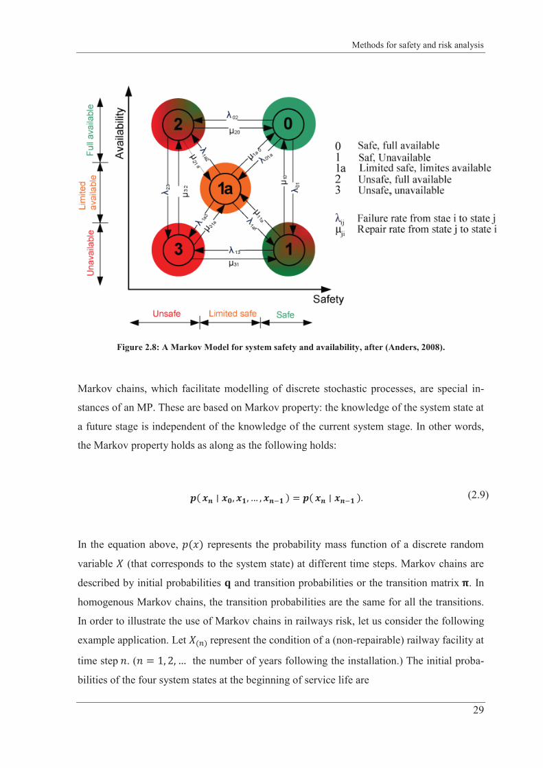
Methods for safety and risk analysis
29
Figure 2.8: A Markov Model for system safety and availability, after (Anders, 2008).
Markov chains, which facilitate modelling of discrete stochastic processes, are special in-
stances of an MP. These are based on Markov property: the knowledge of the system state at
a future stage is independent of the knowledge of the current system stage. In other words,
the Markov property holds as along as the following holds:
(2.9)
In the equation above, represents the probability mass function of a discrete random
variable (that corresponds to the system state) at different time steps. Markov chains are
described by initial probabilities and transition probabilities or the transition matrix . In
homogenous Markov chains, the transition probabilities are the same for all the transitions.
In order to illustrate the use of Markov chains in railways risk, let us consider the following
example application. Let represent the condition of a (non-repairable) railway facility at
time step . ( the number of years following the installation.) The initial proba-
bilities of the four system states at the beginning of service life are
A Bayesian Network Methodology for Railway Risk, Safety and Decision Support
30
(2.10)
In the equation above, the system states 3 and 4 can cause risks on railways and their proba-
bilities are changing w.r.t time. The transition probability matrix that governs the changes
of a state that occur within a system is
(2.11)
In the equation above, is the transition rate from state to state . For example,
is the transition probability of the system in state 3 at time step given that it was in
state in time step . The probability of system failure as a function of time is shown in
Figure 2.9. If one is interested in the failure probability distribution of the railway system
after 25 years, it will be calculated in the following way:
(2.12)
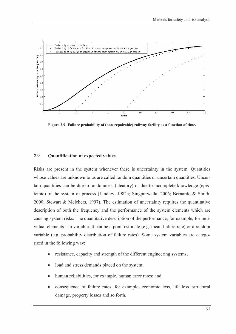
Methods for safety and risk analysis
31
Figure 2.9: Failure probability of (non-repairable) railway facility as a function of time.
2.9 Quantification of expected values
Risks are present in the system whenever there is uncertainty in the system. Quantities
whose values are unknown to us are called random quantities or uncertain quantities. Uncer-
tain quantities can be due to randomness (aleatory) or due to incomplete knowledge (epis-
temic) of the system or process (Lindley, 1982a; Singpurwalla, 2006; Bernardo & Smith,
2000; Stewart & Melchers, 1997). The estimation of uncertainty requires the quantitative
description of both the frequency and the performance of the system elements which are
causing system risks. The quantitative description of the performance, for example, for indi-
vidual elements is a variable. It can be a point estimate (e.g. mean failure rate) or a random
variable (e.g. probability distribution of failure rates). Some system variables are catego-
rized in the following way:
resistance, capacity and strength of the different engineering systems;
load and stress demands placed on the system;
human reliabilities, for example, human error rates; and
consequence of failure rates, for example, economic loss, life loss, structural
damage, property losses and so forth.
A Bayesian Network Methodology for Railway Risk, Safety and Decision Support
32
A point estimate such as the mean value has a single numerical value, which is used to de-
scribe the best estimate of the value of the variable. For example, when fatal accidents are
estimated as 2.1 per billion train-km for UK railways (Evans, 2003), this value is a point
estimate. Point estimates for variables ignore variability (Bowles, 2002). For instance, the
fatal accident rate is not the same for all similar sections of the UK’s railways due to differ-
ent environment, load and maintenance conditions. However, it is assumed to be the same
for all sections at any time during the life of the system in point estimates. Another cause of
variability is uncertainty in the field data due to the lack of understanding of the system, ob-
solescence and so forth. In order to address the variability and uncertainty issues in the data
for the purposes of risk analysis, one should represent variables such as resistance, load and
consequences as random variables, which are characterized by probability distributions. In
this way, for instance, random variables will distribute the variation in fatal accidents evenly
among similar sections of the UK’s railways.
Random variables are described by probability distributions. Probability density function
(PDF), probability mass function (PMF), and cumulative distribution function (CDF) are the
forms of probability distributions for random variables. In probabilistic modelling of ran-
dom variables, a functional form (e.g. Poisson distribution or binomial distribution) is se-
lected and the values of its parameters are determined. The well-known statistical parame-
ters used to describe probabilistic models are first moment (mean, ) and the second mo-
ment (variance, ). The mean provides the best estimates of the value of a random varia-
ble, that is the most likely to occur in practice, whereas, variance provides a measure of un-
certainty associated with this random variable. The simplest way of computing the moments
of a probabilistic model for discrete (Eq. (2.13)) and continuous (Eq. (2.14)) cases are given
in the following.
(2.13)
(2.14)
Methods for safety and risk analysis
33
In the equations above, is the probability of the occurrence of each value of the
random variable and is the PDF for the continuous random variable case. Other
measures are the standard deviation and the coefficient of variance . The stand-
ard deviation shows how much variation there is from the mean whereas is a normalized
measure of the dispersion of a probability distribution. The third moment, skewness, of the
probability distribution provides information about the asymmetry. For further details on the
description and characterization of various random variables see (Benjamin & Cornell,
1970; Ross, 1997) and for their application to risk, safety and reliability see (Rausand &
Hoyland, 2004; Zio, 2007; Kottegoda & Rosso, 2008; Misra, 2008).
Different probability distribution models, for example, binomial, exponential, Poisson, nor-
mal, lognormal, gamma, extreme values for maxima and minima, beta, and others, have
been developed and are used based on the characteristics of the system elements. The ‘mo-
ments’ are the parts of the parameters for different distribution models above. The selection
of probability distribution for the purpose of risk analysis is dependent upon the characteris-
tics of the random variables and the relation by which the risk analyst prefers to describe it.
Some commonly used probability distributions in engineering risk and reliability are given
in (Faber, 2012; Bucher, 2009; Straub, 2011). For example, the (2-parameter) Weibull dis-
tribution is widely used for modelling lifetime distributions in engineering. The PDF of
Weibull is given by:
(2.15)
In the equation above, and are the scale and the shape parameters, respectively. In the
literature, is referred to as the characteristic life. One of the main reasons for this is the
flexibility of the distribution shapes that can be approximated by varying Weibull’s two pa-
rameters . For in the Weibull PDF above, we obtain an exponential distribution,
which is also widely used to model the amount of time until a specific event occurs or to
A Bayesian Network Methodology for Railway Risk, Safety and Decision Support
34
model the time between independent events. The PDF of an exponential distribution with
arrival rate in time t is calculated as
(2.16)
In this way, the first and second moments of an exponential distribution will be and ,
respectively.
Mainly, uncertainty in probabilistic models arises from two error sources: the model inputs
and the models themselves (Benjamin & Cornell, 1970). The reasons for model uncertainty
are: (1) the random variables for the model parameters and (2) the ability of the probabilistic
models to fully describe the characteristics of the system and its elements. Model inputs
cause statistical uncertainty which fails to estimate the model parameters with precision as
they are estimated from a limited amount of data. (Fundamentally, we want more and more
data for improved estimates.) These types of uncertainties can be eliminated by gathering
sufficient data about the events and by making system understanding better. That is why sta-
tistical inference used for parameter estimation establishes probability models based on ob-
servations. Method of Moments (MOM), Maximum Likelihood Estimation (MLE) and
Bayesian analysis (BA) are well-known statistical inference methods used to estimate the
distribution parameters on the basis of data. MOM uses sample mean and variance as point
estimators for the mean and the standard deviation of the random variable. This random var-
iable describes the full population that is represented by the data set. When fitting a para-
metric distribution to a set of data, we equate the sample moments to those of the fitted dis-
tribution in order to estimate the distribution parameters (Kottegoda & Rosso, 2008). For
instance, when a normal distribution ( ) is selected as the functional form of the
probability model the point estimates for the distribution parameters and are simply
(mean of sample) and (standard deviation of sample), respectively.
The MLE method is applied when a random variable X has a known PDF, and ob-
served values , in a random sample of size . The likelihood function of unknown
parameter is
Methods for safety and risk analysis
35
(2.17)
The objective is to maximize for the given data set. This is done by taking as many
partial derivatives of as is equal to the number of parameters in the model, and equat-
ing them to zero. At the end, the MLE of the parameter set are calculated from the solu-
tions of the equations.
2.9.1 Bayesian Analysis – BA
When additional information becomes available, the probability structure in the model may
be updated. This is done by using BA, which is based on Bayes’ theorem (Gelman, et al.,
2009; Koller & Friedman, 2009). This method is particularly useful when the amount of
available data is sparse and the statistical uncertainty is large. In these cases, experimental
data (obtained for a specific plant) and reliability data (obtained from reliability databases or
expert opinions) are combined by using Bayes theorem. This theorem states how prior prob-
abilities, combined with new information from a sample, can be used to update beliefs. The
updated belief is called the posterior probability and is calculated as:
(2.18)
In the equation above is the unknown parameter whereas
is the prior distribution of parameter which represents the data;
is a sample drawn from the underlying distribution which represents the ex-
perimental data;
is the sampling density of and represents the likelihood function or
conditional probability of observing the experimental outcome given the
value of the parameter . Our prior knowledge of the failure data is weighted
A Bayesian Network Methodology for Railway Risk, Safety and Decision Support
36
by the likelihood function, which is regarded as a credibility check on the pri-
or knowledge;
is the posterior distribution of ; and
is a normalizing constant to satisfy the requirement
for the resulting PMF.
DISCRETE FORM OF BAYES’ THEOREM
A simple case of a discrete probability distribution, such as Poisson, is shown to demon-
strate the use of Bayes’ theorem. Let be one failure rate of a set of possible rates of a
component and is evidence. We wish to express our knowledge in terms of . We
want to compute the , which is the probability of given the obser-
vation of 02 failures in a 100 hour operation:
(2.19)
Assuming that is a constant and the likelihood function follows the Poisson distribution:
(2.20)
The calculation of the posterior probability of the desired event for
is shown in Table 2.5. The comparison of the prior and the posterior
knowledge is shown in Figure 2.10. It should be noted that the posterior probability of the
desired event increases after updating.
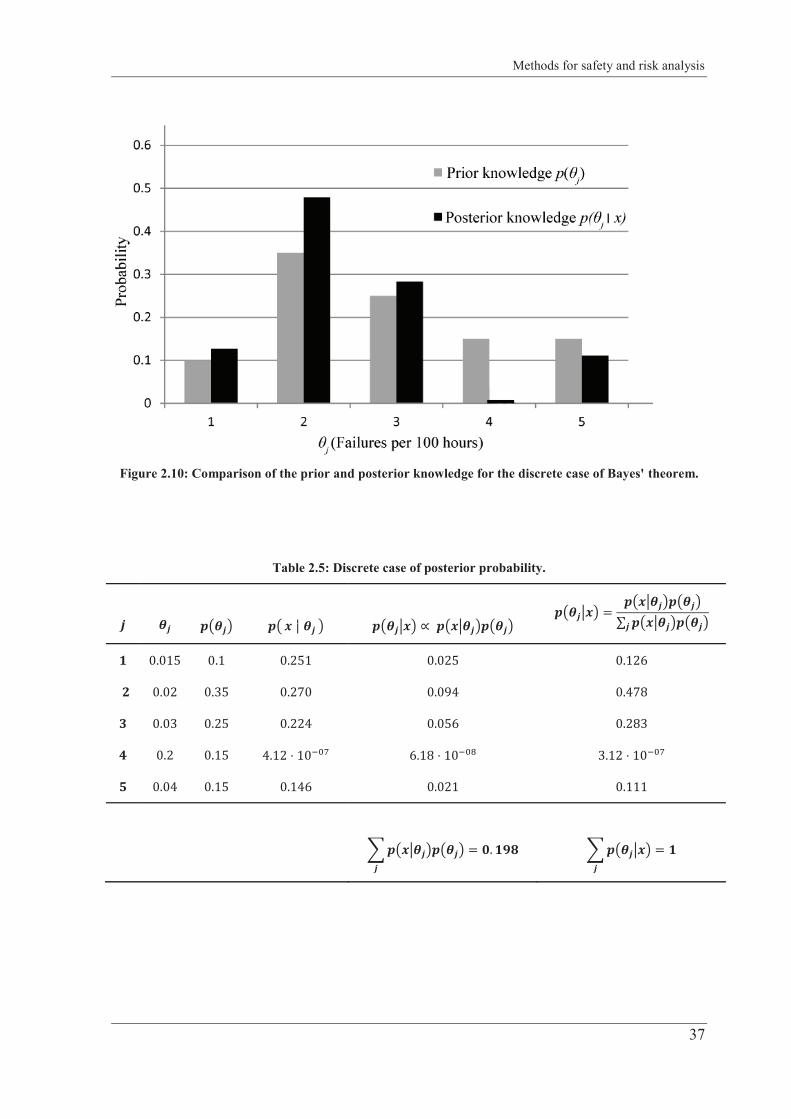
Methods for safety and risk analysis
37
Figure 2.10: Comparison of the prior and posterior knowledge for the discrete case of Bayes' theorem.
Table 2.5: Discrete case of posterior probability.
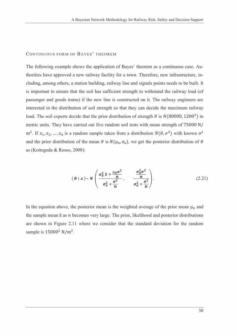
A Bayesian Network Methodology for Railway Risk, Safety and Decision Support
38
CONTINUOUS FORM OF BAYES’ THEOREM
The following example shows the application of Bayes’ theorem as a continuous case. Au-
thorities have approved a new railway facility for a town. Therefore, new infrastructure, in-
cluding, among others, a station building, railway line and signals points needs to be built. It
is important to ensure that the soil has sufficient strength to withstand the railway load (of
passenger and goods trains) if the new line is constructed on it. The railway engineers are
interested in the distribution of soil strength so that they can decide the maximum railway
load. The soil experts decide that the prior distribution of strength is in
metric units. They have carried out five random soil tests with mean strength of
. If is a random sample taken from a distribution with known
and the prior distribution of the mean is , we get the posterior distribution of
as (Kottegoda & Rosso, 2008):
(2.21)
In the equation above, the posterior mean is the weighted average of the prior mean and
the sample mean as becomes very large. The prior, likelihood and posterior distributions
are shown in Figure 2.11 where we consider that the standard deviation for the random
sample is .
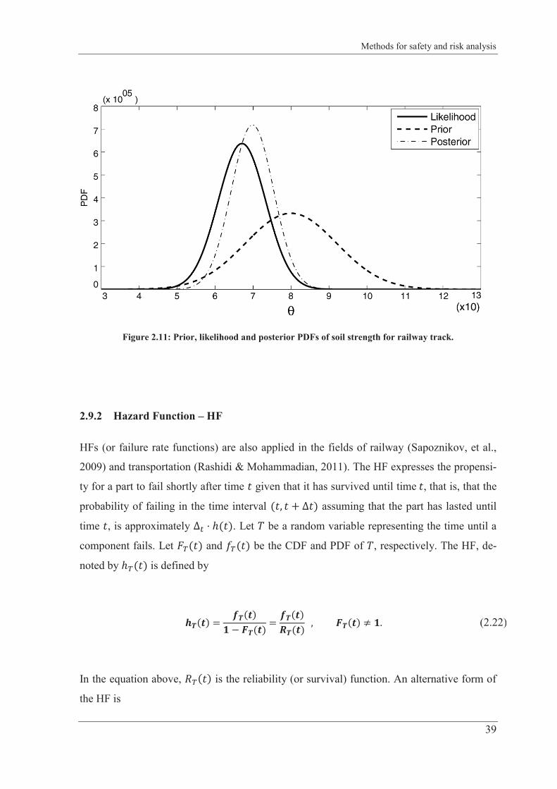
Methods for safety and risk analysis
39
Figure 2.11: Prior, likelihood and posterior PDFs of soil strength for railway track.
2.9.2 Hazard Function – HF
HFs (or failure rate functions) are also applied in the fields of railway (Sapoznikov, et al.,
2009) and transportation (Rashidi & Mohammadian, 2011). The HF expresses the propensi-
ty for a part to fail shortly after time given that it has survived until time , that is, that the
probability of failing in the time interval assuming that the part has lasted until
time , is approximately . Let be a random variable representing the time until a
component fails. Let and be the CDF and PDF of , respectively. The HF, de-
noted by is defined by
(2.22)
In the equation above, is the reliability (or survival) function. An alternative form of
the HF is
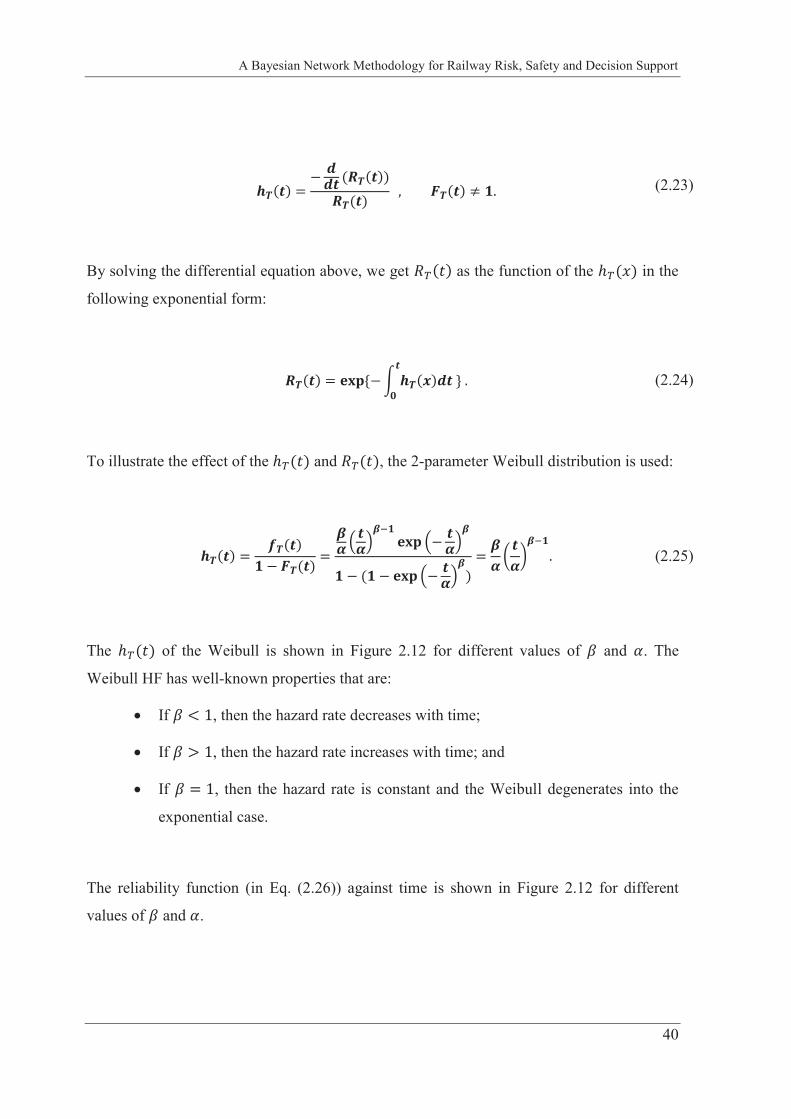
A Bayesian Network Methodology for Railway Risk, Safety and Decision Support
40
(2.23)
By solving the differential equation above, we get as the function of the in the
following exponential form:
(2.24)
To illustrate the effect of the and , the 2-parameter Weibull distribution is used:
(2.25)
The of the Weibull is shown in Figure 2.12 for different values of and . The
Weibull HF has well-known properties that are:
If , then the hazard rate decreases with time;
If , then the hazard rate increases with time; and
If , then the hazard rate is constant and the Weibull degenerates into the
exponential case.
The reliability function (in Eq. (2.26)) against time is shown in Figure 2.12 for different
values of and .
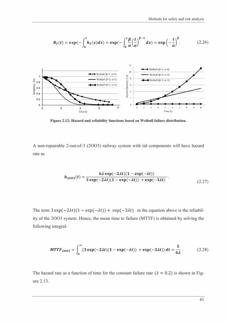
Methods for safety and risk analysis
41
(2.26)
Figure 2.12: Hazard and reliability functions based on Weibull failure distribution.
A non-repairable 2-out-of-3 (2OO3) railway system with iid components will have hazard
rate as
(2.27)
The term in the equation above is the reliabil-
ity of the 2OO3 system. Hence, the mean time to failure (MTTF) is obtained by solving the
following integral:
(2.28)
The hazard rate as a function of time for the constant failure rate is shown in Fig-
ure 2.13.
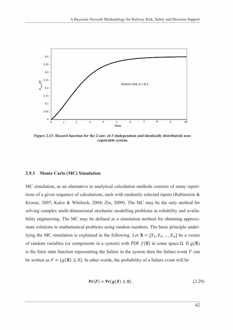
A Bayesian Network Methodology for Railway Risk, Safety and Decision Support
42
Figure 2.13: Hazard function for the 2-out- of-3 (independent and identically distributed) non-repairable system.
2.9.3 Monte Carlo (MC) Simulation
MC simulation, as an alternative to analytical calculation methods consists of many repeti-
tions of a given sequence of calculations, each with randomly selected inputs (Rubinstein &
Kroese, 2007; Kalos & Whitlock, 2004; Zio, 2009). The MC may be the only method for
solving complex multi-dimensional stochastic modelling problems in reliability and availa-
bility engineering. The MC may be defined as a simulation method for obtaining approxi-
mate solutions to mathematical problems using random numbers. The basic principle under-
lying the MC simulation is explained in the following. Let be a vector
of random variables (or components in a system) with PDF in some space . If
is the limit state function representing the failure in the system then the failure event can
be written as . In other words, the probability of a failure event will be
(2.29)
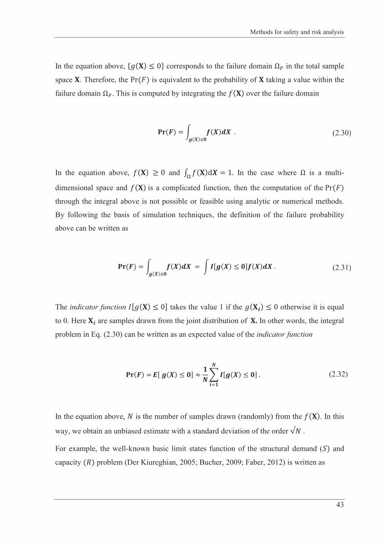
Methods for safety and risk analysis
43
In the equation above, corresponds to the failure domain in the total sample
space . Therefore, the is equivalent to the probability of taking a value within the
failure domain . This is computed by integrating the over the failure domain
(2.30)
In the equation above, and In the case where is a multi-
dimensional space and is a complicated function, then the computation of the
through the integral above is not possible or feasible using analytic or numerical methods.
By following the basis of simulation techniques, the definition of the failure probability
above can be written as
(2.31)
The indicator function takes the value 1 if the otherwise it is equal
to 0. Here are samples drawn from the joint distribution of . In other words, the integral
problem in Eq. (2.30) can be written as an expected value of the indicator function
In the equation above, is the number of samples drawn (randomly) from the . In this
way, we obtain an unbiased estimate with a standard deviation of the order .
For example, the well-known basic limit states function of the structural demand ( and
capacity problem (Der Kiureghian, 2005; Bucher, 2009; Faber, 2012) is written as
(2.32)
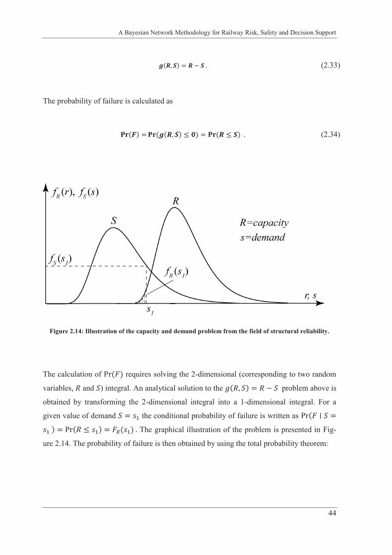
A Bayesian Network Methodology for Railway Risk, Safety and Decision Support
44
The probability of failure is calculated as
Figure 2.14: Illustration of the capacity and demand problem from the field of structural reliability.
The calculation of requires solving the 2-dimensional (corresponding to two random
variables, and ) integral. An analytical solution to the problem above is
obtained by transforming the 2-dimensional integral into a 1-dimensional integral. For a
given value of demand the conditional probability of failure is written as
The graphical illustration of the problem is presented in Fig-
ure 2.14. The probability of failure is then obtained by using the total probability theorem:
(2.33)
(2.34)
Methods for safety and risk analysis
45
In the following, we solve the 2-dimensional integral problem above using MC simulation.
Assume that capacity ( and demand ( follow a Normal distribution (see
Figure 2.15) with parameter values and
, respectively and are uncorrelated. We generate samples of and .
Whether or not the individual sample falls into the failure domain is investigated. We esti-
mate the using the following indicator function
Only samples fall into the failure domain out of the samples. In this way,
The standard deviation of the estimate can be deter-
mined from
(2.35)
(2.36)
(2.37)
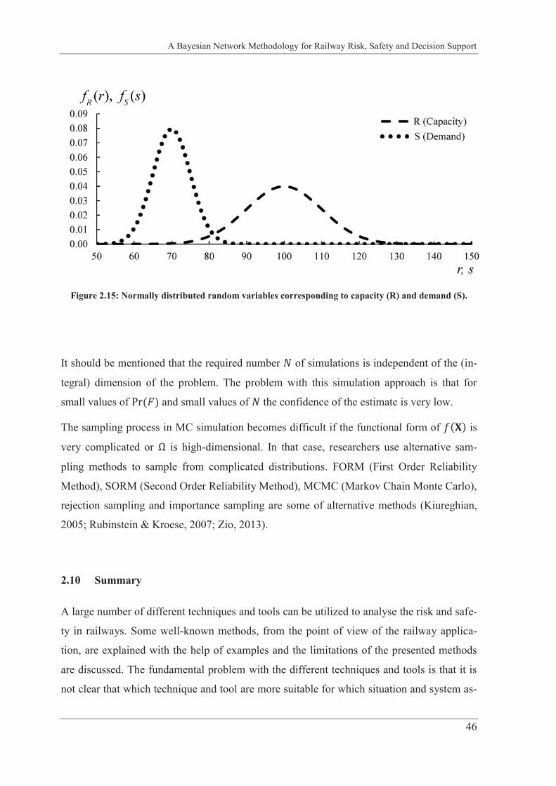
A Bayesian Network Methodology for Railway Risk, Safety and Decision Support
46
Figure 2.15: Normally distributed random variables corresponding to capacity (R) and demand (S).
It should be mentioned that the required number of simulations is independent of the (in-
tegral) dimension of the problem. The problem with this simulation approach is that for
small values of and small values of the confidence of the estimate is very low.
The sampling process in MC simulation becomes difficult if the functional form of is
very complicated or is high-dimensional. In that case, researchers use alternative sam-
pling methods to sample from complicated distributions. FORM (First Order Reliability
Method), SORM (Second Order Reliability Method), MCMC (Markov Chain Monte Carlo),
rejection sampling and importance sampling are some of alternative methods (Kiureghian,
2005; Rubinstein & Kroese, 2007; Zio, 2013).
2.10 Summary
A large number of different techniques and tools can be utilized to analyse the risk and safe-
ty in railways. Some well-known methods, from the point of view of the railway applica-
tion, are explained with the help of examples and the limitations of the presented methods
are discussed. The fundamental problem with the different techniques and tools is that it is
not clear that which technique and tool are more suitable for which situation and system as-
Methods for safety and risk analysis
47
pect. The risk analysis process followed in the different techniques begins with different ac-
tivities, finish with different activities and follow different ways and paths in between be-
ginning and finish. Although every technique and tool are based on different analysis and
evaluation criteria; however, these techniques and tools can be suitable to compare and to
classify safety and risk problems of different railway systems. Qualitative and semi-
quantitative techniques like risk matrix and FMEA compare and classify system safety and
risks mainly based on experience of system experts. Different experts may use different or
even totally opposite ways of modelling the same system (behavior and characteristics) in
qualitative analysis.
Quantitative techniques such as Fault Tree, Event Tree, Markov Model, hazard functions
and Monte Carlo simulation techniques evaluate railway risk and safety based on calcula-
tion results using mathematical models. It is only the quantitative technique, which provides
a mean to compute the parameters related to risk and safety problems. However, the param-
eters of the mathematical models themselves can be highly uncertain.
In conclusion, it can be seen that all methods are not well suited to all kinds of risk and safe-
ty problems, but some are more useful than others (Rouvroye & van den Bliek, 2002;
Braband, 2001). Therefore, care must be taken in the selection of a risk analysis method and
decisions need to be taken on a case-by-case basis. For example, there can be a case when
one analysis technique (say Fault Tree Analysis) is not enough and one needs to use a com-
bination of techniques (say Monte Carlo simulation and Fault Tree Analysis or FMEA and
Fault Tree Analysis.)
CHAPTER 3: INTRODUCTION TO BAYESIAN NETWORKS
This section describes Bayesian Networks, which use a graph-based representation to model
joint distributions of random variables in a compact way. Here, sufficient introduction to
Bayesian Networks is provided so that methods and models presented in the coming chap-
ters can be better understood. For readings on Bayesian Networks and associated topics in
detail, readers are referred to (Jensen & Nielsen, 2007; Koller & Friedman, 2009; Ahmed,
2010; Murphy, 2002). For the application of Bayesian Networks to risk assessment and de-
cision support we refer to (Bensi, 2010; Hanea & Ale, 2009(b); Heredia-Zavoni, et al.,
2012; Spackova & Straub, 2013; Straub, 2009).
3.1 Terminology in Bayesian Networks
Bayesian Networks are directed acyclic probabilistic graphical models that represent joint
probability distribution of all variables in the network. They consist of a set of nodes (el-
lipse), which correspond to discrete or continuous random variables in Bayesian Networks
and a set of directed links (arrows), which represent (probabilistic) dependence structure
among nodes in Bayesian Networks. Consider the Bayesian Networks shown in Figure 3.1
which models dependencies among six random variables . For example, the
random variable is probabilistically dependent on the variables and . In Bayesi-
an Networks the nodes are the children of , which is parent of the formers. The
variables and have no parents and the variables and have no children. If the
Bayesian Networks consist of discrete random variables then each node will have a set of
mutually exclusive and collective exhaustive states. A conditional probability table (CPT) is
attached to child random variables. The CPT is utilized to describe the conditional probabil-
ity mass function of a discrete random variable, given each of the mutually exclusive states
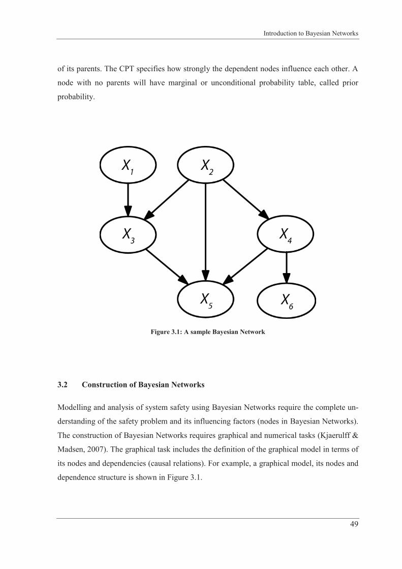
Introduction to Bayesian Networks
49
of its parents. The CPT specifies how strongly the dependent nodes influence each other. A
node with no parents will have marginal or unconditional probability table, called prior
probability.
Figure 3.1: A sample Bayesian Network
3.2 Construction of Bayesian Networks
Modelling and analysis of system safety using Bayesian Networks require the complete un-
derstanding of the safety problem and its influencing factors (nodes in Bayesian Networks).
The construction of Bayesian Networks requires graphical and numerical tasks (Kjaerulff &
Madsen, 2007). The graphical task includes the definition of the graphical model in terms of
its nodes and dependencies (causal relations). For example, a graphical model, its nodes and
dependence structure is shown in Figure 3.1.
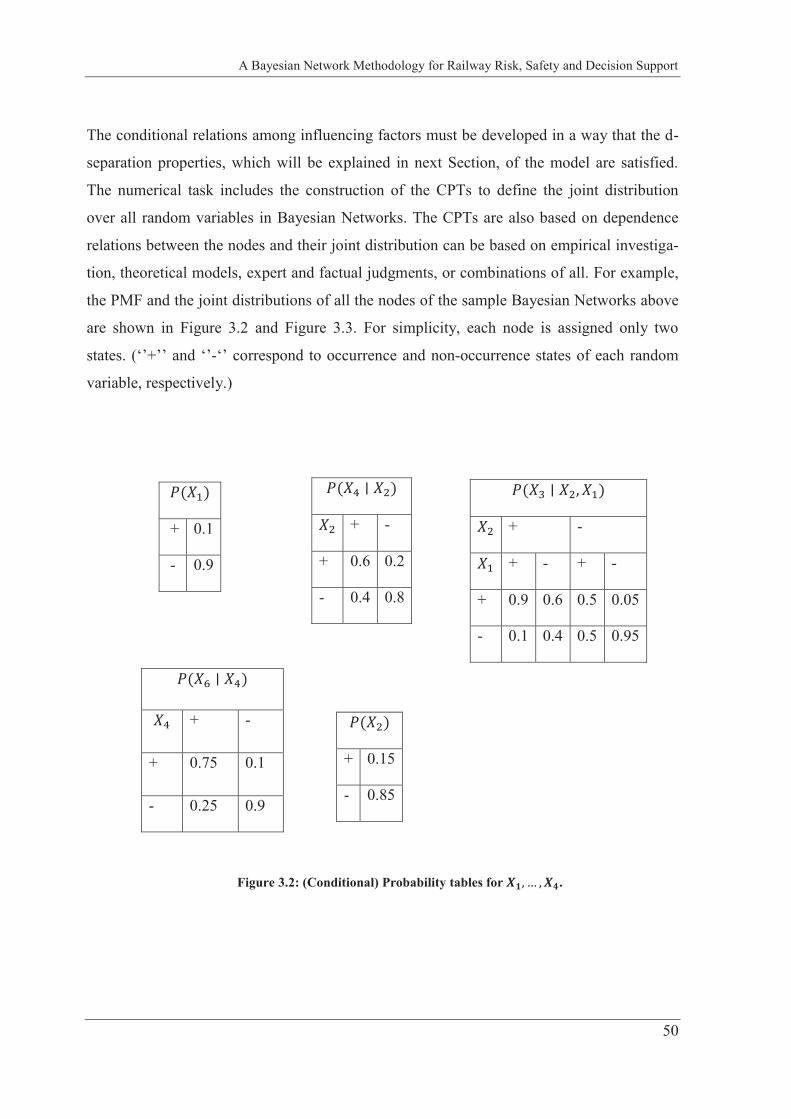
A Bayesian Network Methodology for Railway Risk, Safety and Decision Support
50
The conditional relations among influencing factors must be developed in a way that the d-
separation properties, which will be explained in next Section, of the model are satisfied.
The numerical task includes the construction of the CPTs to define the joint distribution
over all random variables in Bayesian Networks. The CPTs are also based on dependence
relations between the nodes and their joint distribution can be based on empirical investiga-
tion, theoretical models, expert and factual judgments, or combinations of all. For example,
the PMF and the joint distributions of all the nodes of the sample Bayesian Networks above
are shown in Figure 3.2 and Figure 3.3. For simplicity, each node is assigned only two
states. (‘’+’’ and ‘’-‘’ correspond to occurrence and non-occurrence states of each random
variable, respectively.)
+ 0.15
- 0.85
+ -
+ - + -
+ 0.9 0.6 0.5 0.05
- 0.1 0.4 0.5 0.95
+ -
+ 0.6 0.2
- 0.4 0.8
+ -
+ 0.75 0.1
- 0.25 0.9
+ 0.1
- 0.9
Figure 3.2: (Conditional) Probability tables for .
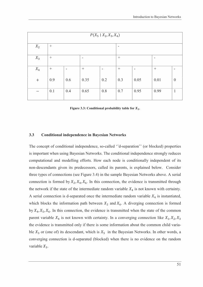
Introduction to Bayesian Networks
51
+ -
+ - + -
+ - + - + - + -
0.9 0.6 0.35 0.2 0.3 0.05 0.01 0
0.1 0.4 0.65 0.8 0.7 0.95 0.99 1
Figure 3.3: Conditional probability table for .
3.3 Conditional independence in Bayesian Networks
The concept of conditional independence, so-called ‘’d-separation’’ (or blocked) properties
is important when using Bayesian Networks. The conditional independence strongly reduces
computational and modelling efforts. How each node is conditionally independent of its
non-descendants given its predecessors, called its parents, is explained below. Consider
three types of connections (see Figure 3.4) in the sample Bayesian Networks above. A serial
connection is formed by . In this connection, the evidence is transmitted through
the network if the state of the intermediate random variable is not known with certainty.
A serial connection is d-separated once the intermediate random variable is instantiated,
which blocks the information path between and . A diverging connection is formed
by . In this connection, the evidence is transmitted when the state of the common
parent variable is not known with certainty. In a converging connection like
the evidence is transmitted only if there is some information about the common child varia-
ble or (one of) its descendant, which is in the Bayesian Networks. In other words, a
converging connection is d-separated (blocked) when there is no evidence on the random
variable .
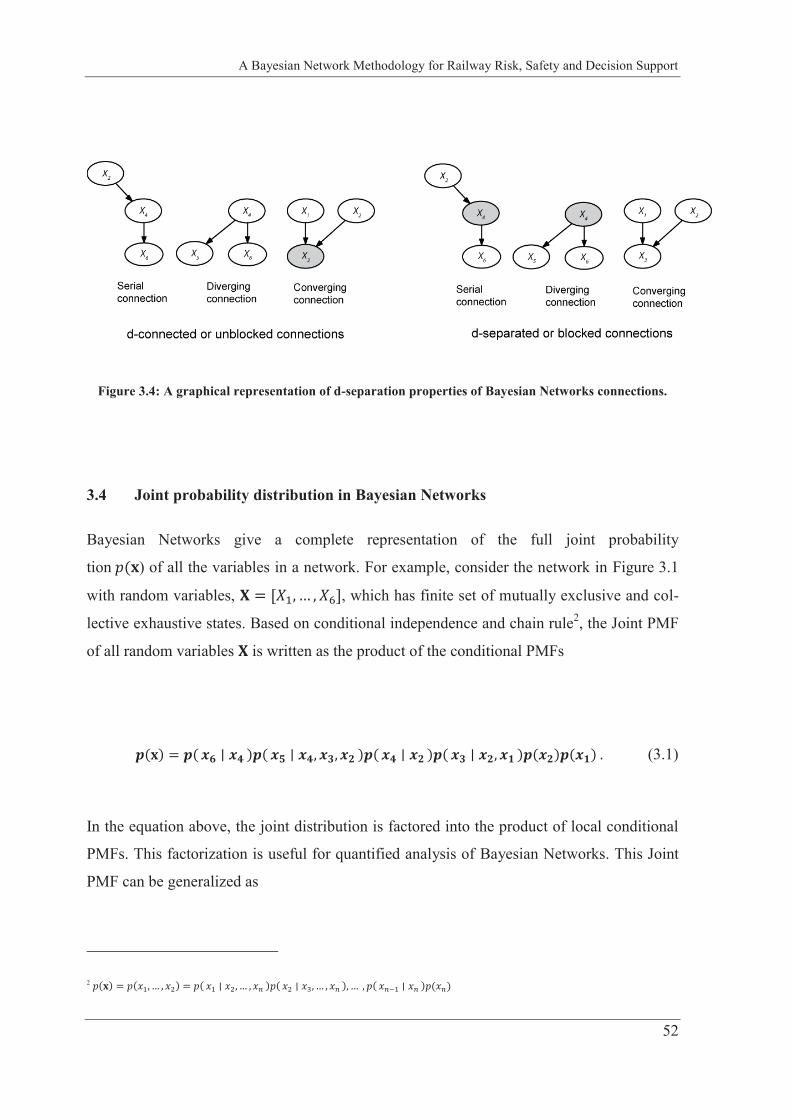
A Bayesian Network Methodology for Railway Risk, Safety and Decision Support
52
Figure 3.4: A graphical representation of d-separation properties of Bayesian Networks connections.
3.4 Joint probability distribution in Bayesian Networks
Bayesian Networks give a complete representation of the full joint probability
tion ) of all the variables in a network. For example, consider the network in Figure 3.1
with random variables, , which has finite set of mutually exclusive and col-
lective exhaustive states. Based on conditional independence and chain rule2, the Joint PMF
of all random variables is written as the product of the conditional PMFs
In the equation above, the joint distribution is factored into the product of local conditional
PMFs. This factorization is useful for quantified analysis of Bayesian Networks. This Joint
PMF can be generalized as
2
(3.1)
Introduction to Bayesian Networks
53
In the generalized form above, is the set of parents of random variables . Bayesian
Networks have advantages that they can perform tasks related to state (1) prediction (for-
ward analysis) using total probability theorem and (2) estimation or diagnostic (backward
analysis) using Bayes’ rule.
3.5 Probabilistic Inference in Bayesian Networks
By making use of Bayesian Networks one can perform three tasks – structural learning (SL),
parameter learning (PL), and probabilistic inference (PI). SL and PL are data driven pro-
cesses. In SL, algorithms determine the topology of the model like number of arrows and
their directions in Bayesian Networks. In PL, unknown parameters of the joint or condition-
al distributions in Bayesian Networks are determined from data using algorithms like Ex-
pectation Maximization (EM) algorithm. For more details on SL and PL we refer to (Jensen
& Nielsen, 2007; Koller & Friedman, 2009; Russel & Norvig, 2010). PI is used to compute
the probability distributions for a set of variables, given some evidence. In this work, Bayes-
ian Networks are used only for PI.
A number of questions related to probability of (set of) variables in Bayesian Networks can
be answered using PI. Consider the network in Figure 3.1 where all random variables have
states. (+ and – represent the occurrence and nonoccurrence states of the binary ran-
dom variables in the Bayesian Networks, respectively.) Mainly, we answer questions like:
what is the probability (of a set) of random variables being in a specific state, say +, giv-
en that another (set of) random variables is observed to be equal to +:
This question can be answered by following conditional probability,
(3.2)
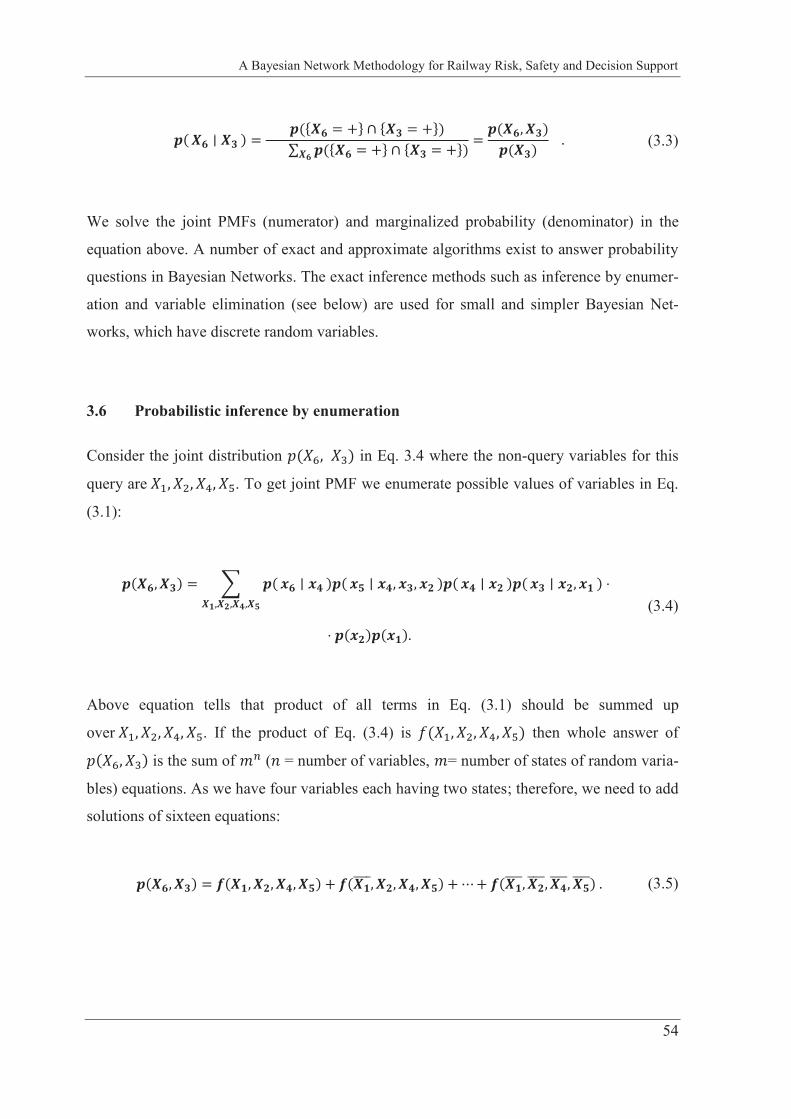
A Bayesian Network Methodology for Railway Risk, Safety and Decision Support
54
We solve the joint PMFs (numerator) and marginalized probability (denominator) in the
equation above. A number of exact and approximate algorithms exist to answer probability
questions in Bayesian Networks. The exact inference methods such as inference by enumer-
ation and variable elimination (see below) are used for small and simpler Bayesian Net-
works, which have discrete random variables.
3.6 Probabilistic inference by enumeration
Consider the joint distribution in Eq. 3.4 where the non-query variables for this
query are . To get joint PMF we enumerate possible values of variables in Eq.
(3.1):
Above equation tells that product of all terms in Eq. (3.1) should be summed up
over . If the product of Eq. (3.4) is then whole answer of
is the sum of ( = number of variables, = number of states of random varia-
bles) equations. As we have four variables each having two states; therefore, we need to add
solutions of sixteen equations:
(3.3)
(3.4)
(3.5)
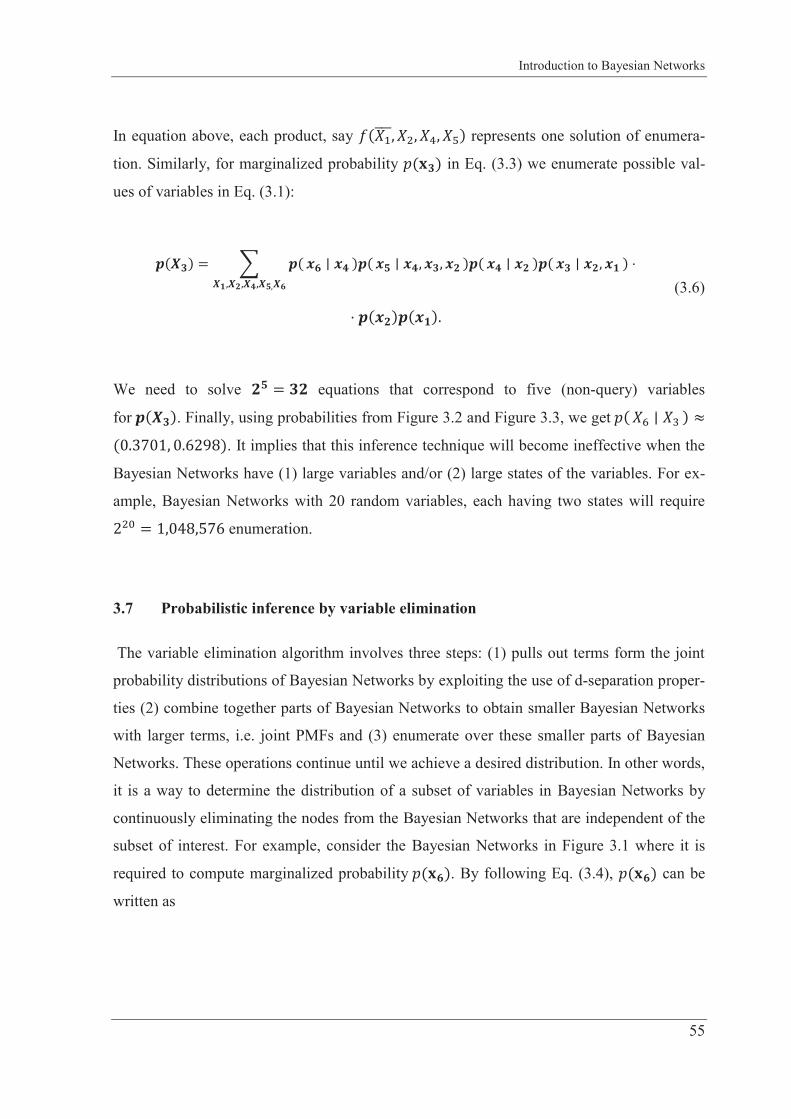
Introduction to Bayesian Networks
55
In equation above, each product, say represents one solution of enumera-
tion. Similarly, for marginalized probability in Eq. (3.3) we enumerate possible val-
ues of variables in Eq. (3.1):
We need to solve equations that correspond to five (non-query) variables
for . Finally, using probabilities from Figure 3.2 and Figure 3.3, we get
. It implies that this inference technique will become ineffective when the
Bayesian Networks have (1) large variables and/or (2) large states of the variables. For ex-
ample, Bayesian Networks with 20 random variables, each having two states will require
enumeration.
3.7 Probabilistic inference by variable elimination
The variable elimination algorithm involves three steps: (1) pulls out terms form the joint
probability distributions of Bayesian Networks by exploiting the use of d-separation proper-
ties (2) combine together parts of Bayesian Networks to obtain smaller Bayesian Networks
with larger terms, i.e. joint PMFs and (3) enumerate over these smaller parts of Bayesian
Networks. These operations continue until we achieve a desired distribution. In other words,
it is a way to determine the distribution of a subset of variables in Bayesian Networks by
continuously eliminating the nodes from the Bayesian Networks that are independent of the
subset of interest. For example, consider the Bayesian Networks in Figure 3.1 where it is
required to compute marginalized probability . By following Eq. (3.4), can be
written as
(3.6)
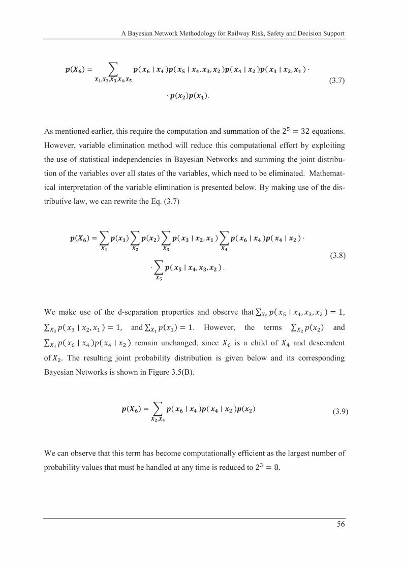
A Bayesian Network Methodology for Railway Risk, Safety and Decision Support
56
As mentioned earlier, this require the computation and summation of the equations.
However, variable elimination method will reduce this computational effort by exploiting
the use of statistical independencies in Bayesian Networks and summing the joint distribu-
tion of the variables over all states of the variables, which need to be eliminated. Mathemat-
ical interpretation of the variable elimination is presented below. By making use of the dis-
tributive law, we can rewrite the Eq. (3.7)
We make use of the d-separation properties and observe that ,
and . However, the terms and
remain unchanged, since is a child of and descendent
of . The resulting joint probability distribution is given below and its corresponding
Bayesian Networks is shown in Figure 3.5(B).
We can observe that this term has become computationally efficient as the largest number of
probability values that must be handled at any time is reduced to
(3.7)
(3.8)
(3.9)
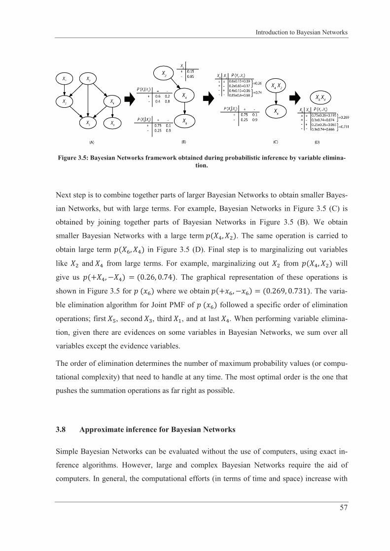
Introduction to Bayesian Networks
57
Figure 3.5: Bayesian Networks framework obtained during probabilistic inference by variable elimina-tion.
Next step is to combine together parts of larger Bayesian Networks to obtain smaller Bayes-
ian Networks, but with large terms. For example, Bayesian Networks in Figure 3.5 (C) is
obtained by joining together parts of Bayesian Networks in Figure 3.5 (B). We obtain
smaller Bayesian Networks with a large term . The same operation is carried to
obtain large term in Figure 3.5 (D). Final step is to marginalizing out variables
like and from large terms. For example, marginalizing out from will
give us . The graphical representation of these operations is
shown in Figure 3.5 for where we obtain . The varia-
ble elimination algorithm for Joint PMF of followed a specific order of elimination
operations; first , second , third , and at last . When performing variable elimina-
tion, given there are evidences on some variables in Bayesian Networks, we sum over all
variables except the evidence variables.
The order of elimination determines the number of maximum probability values (or compu-
tational complexity) that need to handle at any time. The most optimal order is the one that
pushes the summation operations as far right as possible.
3.8 Approximate inference for Bayesian Networks
Simple Bayesian Networks can be evaluated without the use of computers, using exact in-
ference algorithms. However, large and complex Bayesian Networks require the aid of
computers. In general, the computational efforts (in terms of time and space) increase with
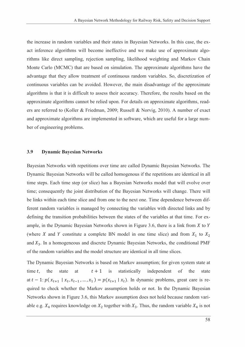
A Bayesian Network Methodology for Railway Risk, Safety and Decision Support
58
the increase in random variables and their states in Bayesian Networks. In this case, the ex-
act inference algorithms will become ineffective and we make use of approximate algo-
rithms like direct sampling, rejection sampling, likelihood weighting and Markov Chain
Monte Carlo (MCMC) that are based on simulation. The approximate algorithms have the
advantage that they allow treatment of continuous random variables. So, discretization of
continuous variables can be avoided. However, the main disadvantage of the approximate
algorithms is that it is difficult to assess their accuracy. Therefore, the results based on the
approximate algorithms cannot be relied upon. For details on approximate algorithms, read-
ers are referred to (Koller & Friedman, 2009; Russell & Norvig, 2010). A number of exact
and approximate algorithms are implemented in software, which are useful for a large num-
ber of engineering problems.
3.9 Dynamic Bayesian Networks
Bayesian Networks with repetitions over time are called Dynamic Bayesian Networks. The
Dynamic Bayesian Networks will be called homogenous if the repetitions are identical in all
time steps. Each time step (or slice) has a Bayesian Networks model that will evolve over
time; consequently the joint distribution of the Bayesian Networks will change. There will
be links within each time slice and from one to the next one. Time dependence between dif-
ferent random variables is managed by connecting the variables with directed links and by
defining the transition probabilities between the states of the variables at that time. For ex-
ample, in the Dynamic Bayesian Networks shown in Figure 3.6, there is a link from to
(where and constitute a complete BN model in one time slice) and from to
and . In a homogeneous and discrete Dynamic Bayesian Networks, the conditional PMF
of the random variables and the model structure are identical in all time slices.
The Dynamic Bayesian Networks is based on Markov assumption; for given system state at
time , the state at is statistically independent of the state
at : . In dynamic problems, great care is re-
quired to check whether the Markov assumption holds or not. In the Dynamic Bayesian
Networks shown in Figure 3.6, this Markov assumption does not hold because random vari-
able e.g. requires knowledge on together with . Thus, the random variable is not
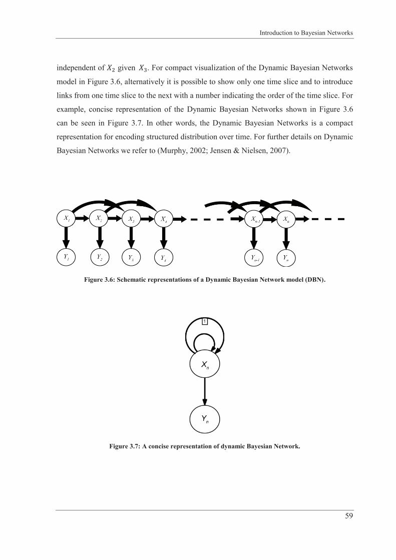
Introduction to Bayesian Networks
59
independent of given . For compact visualization of the Dynamic Bayesian Networks
model in Figure 3.6, alternatively it is possible to show only one time slice and to introduce
links from one time slice to the next with a number indicating the order of the time slice. For
example, concise representation of the Dynamic Bayesian Networks shown in Figure 3.6
can be seen in Figure 3.7. In other words, the Dynamic Bayesian Networks is a compact
representation for encoding structured distribution over time. For further details on Dynamic
Bayesian Networks we refer to (Murphy, 2002; Jensen & Nielsen, 2007).
Figure 3.6: Schematic representations of a Dynamic Bayesian Network model (DBN).
Figure 3.7: A concise representation of dynamic Bayesian Network.
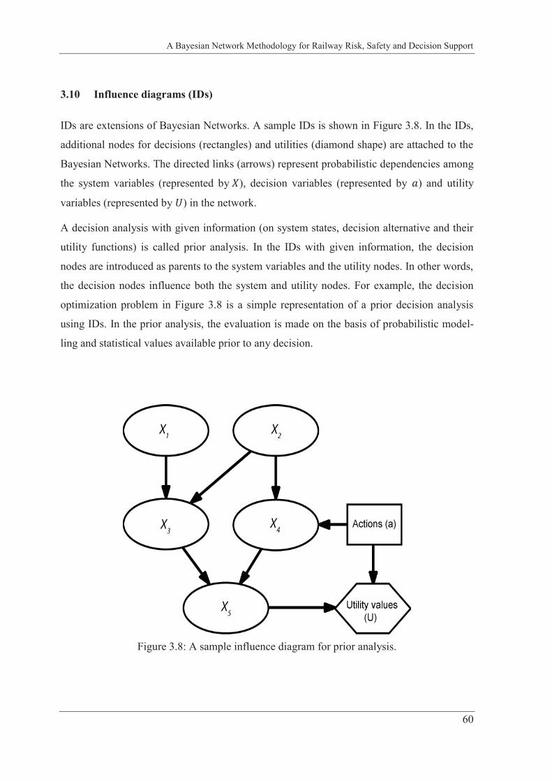
A Bayesian Network Methodology for Railway Risk, Safety and Decision Support
60
3.10 Influence diagrams (IDs)
IDs are extensions of Bayesian Networks. A sample IDs is shown in Figure 3.8. In the IDs,
additional nodes for decisions (rectangles) and utilities (diamond shape) are attached to the
Bayesian Networks. The directed links (arrows) represent probabilistic dependencies among
the system variables (represented by ), decision variables (represented by ) and utility
variables (represented by ) in the network.
A decision analysis with given information (on system states, decision alternative and their
utility functions) is called prior analysis. In the IDs with given information, the decision
nodes are introduced as parents to the system variables and the utility nodes. In other words,
the decision nodes influence both the system and utility nodes. For example, the decision
optimization problem in Figure 3.8 is a simple representation of a prior decision analysis
using IDs. In the prior analysis, the evaluation is made on the basis of probabilistic model-
ling and statistical values available prior to any decision.
Figure 3.8: A sample influence diagram for prior analysis.
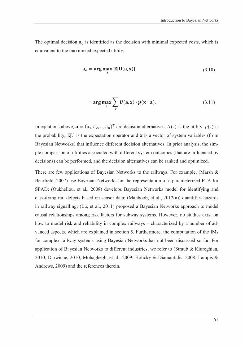
Introduction to Bayesian Networks
61
The optimal decision is identified as the decision with minimal expected costs, which is
equivalent to the maximized expected utility,
In equations above, are decision alternatives, is the utility, is
the probability, [.] is the expectation operator and is a vector of system variables (from
Bayesian Networks) that influence different decision alternatives. In prior analysis, the sim-
ple comparison of utilities associated with different system outcomes (that are influenced by
decisions) can be performed, and the decision alternatives can be ranked and optimized.
There are few applications of Bayesian Networks to the railways. For example, (Marsh &
Bearfield, 2007) use Bayesian Networks for the representation of a parameterized FTA for
SPAD; (Oukhellou, et al., 2008) develops Bayesian Networks model for identifying and
classifying rail defects based on sensor data; (Mahboob, et al., 2012(a)) quantifies hazards
in railway signalling; (Lu, et al., 2011) proposed a Bayesian Networks approach to model
causal relationships among risk factors for subway systems. However, no studies exist on
how to model risk and reliability in complex railways – characterized by a number of ad-
vanced aspects, which are explained in section 5. Furthermore, the computation of the IMs
for complex railway systems using Bayesian Networks has not been discussed so far. For
application of Bayesian Networks to different industries, we refer to (Straub & Kiureghian,
2010; Darwiche, 2010; Mohaghegh, et al., 2009; Holicky & Diamantidis, 2008; Lampis &
Andrews, 2009) and the references therein.
(3.10)
(3.11)
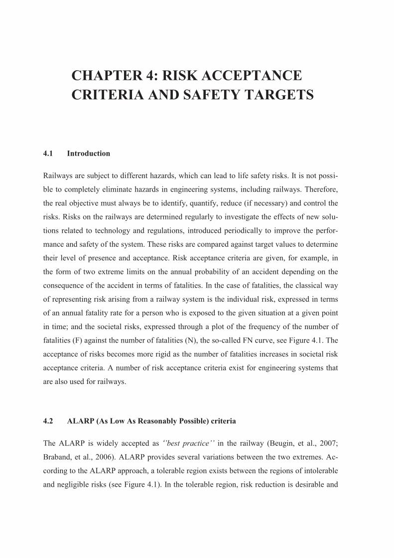
CHAPTER 4: RISK ACCEPTANCE CRITERIA AND SAFETY TARGETS
4.1 Introduction
Railways are subject to different hazards, which can lead to life safety risks. It is not possi-
ble to completely eliminate hazards in engineering systems, including railways. Therefore,
the real objective must always be to identify, quantify, reduce (if necessary) and control the
risks. Risks on the railways are determined regularly to investigate the effects of new solu-
tions related to technology and regulations, introduced periodically to improve the perfor-
mance and safety of the system. These risks are compared against target values to determine
their level of presence and acceptance. Risk acceptance criteria are given, for example, in
the form of two extreme limits on the annual probability of an accident depending on the
consequence of the accident in terms of fatalities. In the case of fatalities, the classical way
of representing risk arising from a railway system is the individual risk, expressed in terms
of an annual fatality rate for a person who is exposed to the given situation at a given point
in time; and the societal risks, expressed through a plot of the frequency of the number of
fatalities (F) against the number of fatalities (N), the so-called FN curve, see Figure 4.1. The
acceptance of risks becomes more rigid as the number of fatalities increases in societal risk
acceptance criteria. A number of risk acceptance criteria exist for engineering systems that
are also used for railways.
4.2 ALARP (As Low As Reasonably Possible) criteria
The ALARP is widely accepted as ‘’best practice’’ in the railway (Beugin, et al., 2007;
Braband, et al., 2006). ALARP provides several variations between the two extremes. Ac-
cording to the ALARP approach, a tolerable region exists between the regions of intolerable
and negligible risks (see Figure 4.1). In the tolerable region, risk reduction is desirable and
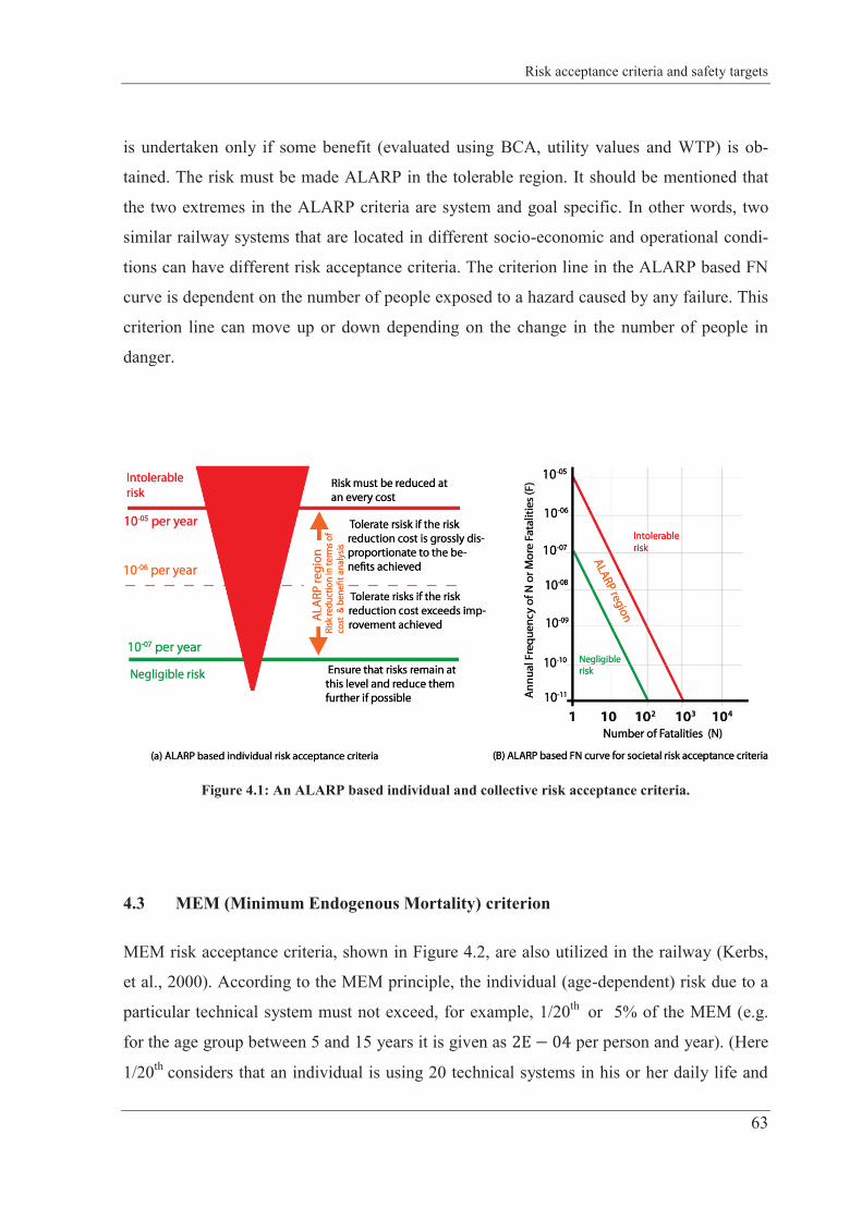
Risk acceptance criteria and safety targets
63
is undertaken only if some benefit (evaluated using BCA, utility values and WTP) is ob-
tained. The risk must be made ALARP in the tolerable region. It should be mentioned that
the two extremes in the ALARP criteria are system and goal specific. In other words, two
similar railway systems that are located in different socio-economic and operational condi-
tions can have different risk acceptance criteria. The criterion line in the ALARP based FN
curve is dependent on the number of people exposed to a hazard caused by any failure. This
criterion line can move up or down depending on the change in the number of people in
danger.
Figure 4.1: An ALARP based individual and collective risk acceptance criteria.
4.3 MEM (Minimum Endogenous Mortality) criterion
MEM risk acceptance criteria, shown in Figure 4.2, are also utilized in the railway (Kerbs,
et al., 2000). According to the MEM principle, the individual (age-dependent) risk due to a
particular technical system must not exceed, for example, 1/20th or 5% of the MEM (e.g.
for the age group between 5 and 15 years it is given as per person and year). (Here
1/20th considers that an individual is using 20 technical systems in his or her daily life and
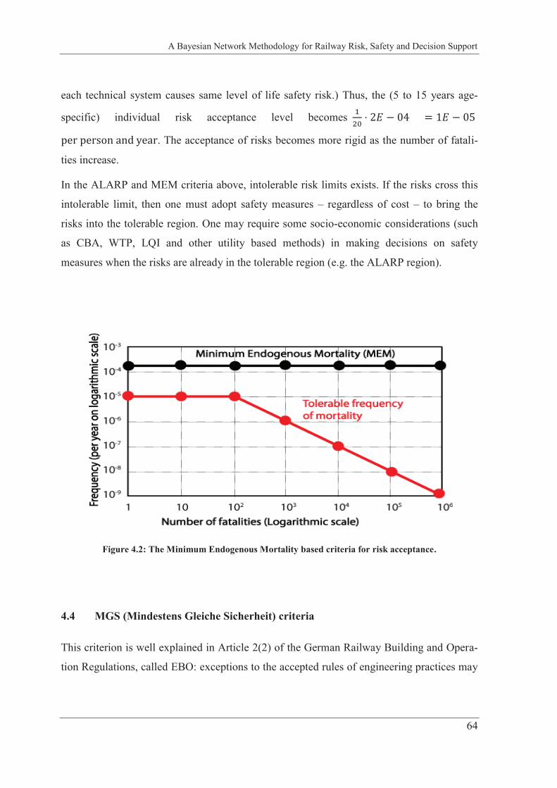
A Bayesian Network Methodology for Railway Risk, Safety and Decision Support
64
each technical system causes same level of life safety risk.) Thus, the (5 to 15 years age-
specific) individual risk acceptance level becomes
. The acceptance of risks becomes more rigid as the number of fatali-
ties increase.
In the ALARP and MEM criteria above, intolerable risk limits exists. If the risks cross this
intolerable limit, then one must adopt safety measures – regardless of cost – to bring the
risks into the tolerable region. One may require some socio-economic considerations (such
as CBA, WTP, LQI and other utility based methods) in making decisions on safety
measures when the risks are already in the tolerable region (e.g. the ALARP region).
Figure 4.2: The Minimum Endogenous Mortality based criteria for risk acceptance.
4.4 MGS (Mindestens Gleiche Sicherheit) criteria
This criterion is well explained in Article 2(2) of the German Railway Building and Opera-
tion Regulations, called EBO: exceptions to the accepted rules of engineering practices may
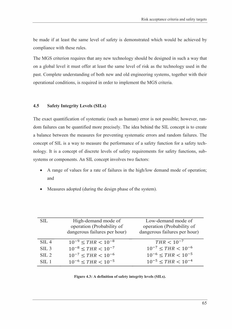
Risk acceptance criteria and safety targets
65
be made if at least the same level of safety is demonstrated which would be achieved by
compliance with these rules.
The MGS criterion requires that any new technology should be designed in such a way that
on a global level it must offer at least the same level of risk as the technology used in the
past. Complete understanding of both new and old engineering systems, together with their
operational conditions, is required in order to implement the MGS criteria.
4.5 Safety Integrity Levels (SILs)
The exact quantification of systematic (such as human) error is not possible; however, ran-
dom failures can be quantified more precisely. The idea behind the SIL concept is to create
a balance between the measures for preventing systematic errors and random failures. The
concept of SIL is a way to measure the performance of a safety function for a safety tech-
nology. It is a concept of discrete levels of safety requirements for safety functions, sub-
systems or components. An SIL concept involves two factors:
A range of values for a rate of failures in the high/low demand mode of operation;
and
Measures adopted (during the design phase of the system).
Figure 4.3: A definition of safety integrity levels (SILs).
SIL High-demand mode of operation (Probability of
dangerous failures per hour)
Low-demand mode of operation (Probability of
dangerous failures per hour)
SIL 4 SIL 3 SIL 2 SIL 1
A Bayesian Network Methodology for Railway Risk, Safety and Decision Support
66
The SIL definitions in Figure 4.3 are adopted from EN 50128 (Railway applications: soft-
ware for railway control and application), EN 50129 (Railway applications: safety related
electronic systems for signalling), IEC 61508 (Functional safety of electri-
cal/electronic/programmable systems) and CENELEC (European Committee for Electro-
technical Standardization) standards (IEC 61508, 2000; CENELEC, 2012). Level 4 and lev-
el 1 correspond to the highest and lowest safety requirements, respectively. An SIL can be
assigned to the safety relevant functions of a sub-system or component of a system. We ap-
ply the SIL concept in the identification of the safety requirements for a PSD system and its
safety functions, see Chapter 6.
4.6 Importance Measures (IMs)
The idea of IMs was first introduced by Birnbaum (Birnbaum, 1969). It is based on the fact
that, usually, not all components contribute to system risk, safety and reliability in the same
way, but some components are relatively more important than others. Therefore, the com-
ponents with higher importance should be treated carefully in the design, maintenance and
operation phases of a system. The IMs can be used to rank the components of a system ac-
cording to their importance. There are two classes of IM, based on structural and reliability
importance. The structural importance measure (SIM) considers the importance of a com-
ponent due to its position in the system and is not concerned about its reliability. So, SIM
cannot classify the components that occupy similar structural positions but have different
reliabilities. The reliability importance measure (RIM) not only considers the position of the
component in the system but the reliability of the component also.
A number of IMs exist that can be used to rank important components (Birnbaum, 1969;
Fussell, 1975; Borgonovo, et al., 2003; Borgonovo & Apostolakis, 2001). For instance, FV
and RAW are commonly used IMs in the nuclear industry (U.S.N.R.C, 2012; Kang, et al.,
2002). RAW identifies the increase in the system risks if a particular component failure in
the system has occurred. The FV gives the fractional contribution of a component failure
towards the system failure. The increase in the occurrence probability of the component
failure will lead to the increase in the FV value. For instance, the NRC regulatory guide
1.174 suggests an FV of 0.05 at the system level and 0.005 at the component level for nu-
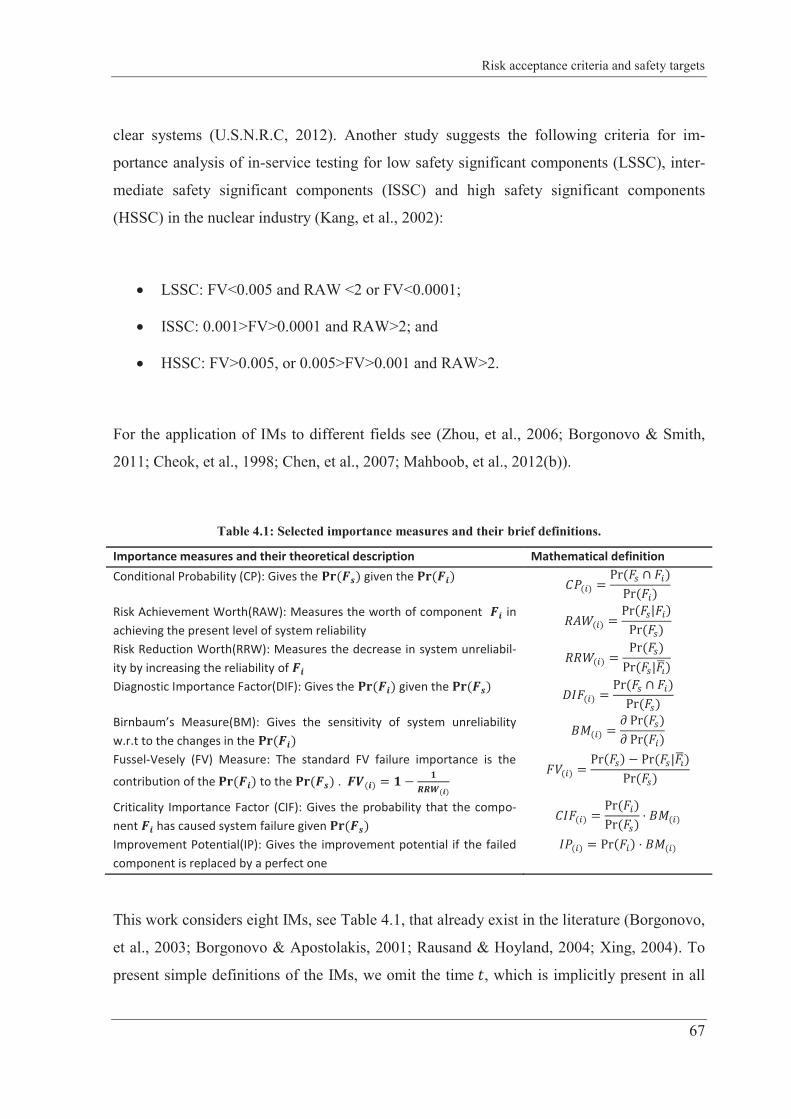
Risk acceptance criteria and safety targets
67
clear systems (U.S.N.R.C, 2012). Another study suggests the following criteria for im-
portance analysis of in-service testing for low safety significant components (LSSC), inter-
mediate safety significant components (ISSC) and high safety significant components
(HSSC) in the nuclear industry (Kang, et al., 2002):
LSSC: FV<0.005 and RAW <2 or FV<0.0001;
ISSC: 0.001>FV>0.0001 and RAW>2; and
HSSC: FV>0.005, or 0.005>FV>0.001 and RAW>2.
For the application of IMs to different fields see (Zhou, et al., 2006; Borgonovo & Smith,
2011; Cheok, et al., 1998; Chen, et al., 2007; Mahboob, et al., 2012(b)).
Table 4.1: Selected importance measures and their brief definitions.
Importance measures and their theoretical description Mathematical definition Conditional Probability (CP): Gives the given the
Risk Achievement Worth(RAW): Measures the worth of component in achieving the present level of system reliability
Risk Reduction Worth(RRW): Measures the decrease in system unreliabil-ity by increasing the reliability of
Diagnostic Importance Factor(DIF): Gives the given the
Birnbaum’s Measure(BM): Gives the sensitivity of system unreliability w.r.t to the changes in the
Fussel-Vesely (FV) Measure: The standard FV failure importance is the
contribution of the to the .
Criticality Importance Factor (CIF): Gives the probability that the compo-nent has caused system failure given
Improvement Potential(IP): Gives the improvement potential if the failed component is replaced by a perfect one
This work considers eight IMs, see Table 4.1, that already exist in the literature (Borgonovo,
et al., 2003; Borgonovo & Apostolakis, 2001; Rausand & Hoyland, 2004; Xing, 2004). To
present simple definitions of the IMs, we omit the time , which is implicitly present in all
A Bayesian Network Methodology for Railway Risk, Safety and Decision Support
68
of the definitions given in Table 4.1. In the definitions, denotes the probability of the
failure of a system, which is computed as a function of the probability of the component de-
noted by .
4.7 Life Quality Index (LQI)
The problem of risk acceptance turns into an economic decision problem when the risks are
in the so-called ALARP region (see Figure 4.1) and the objective is to further reduce the
risks. For example, should we introduce a safety measure if the individual risk is just close
to the risk acceptance level? In this situation one requires additional criteria, which may be
based on socio-economic considerations. It implies that the considerations of (changing)
socio-economic conditions and accommodation of additional information on factual
knowledge, which becomes available over time, can affect the decision-making process. For
example, the gross domestic product (GDP) per person, and the life expectancy of a human
exposed to danger are important socio-economic indicators. Moreover, one safety measure
can be a better alternative in terms of value for money and performance than other safety
measures. In this situation, socio-economic considerations such as BCA have been utilized
for railway risks. The profitability of a safety technology by quantifying the WTP (from the
society point of view) is calculated in a BCA. The WTP is the amount that people are will-
ing to pay to save a human life. The BCA and the WTP approaches are usually accepted
methods for valuing the prevention of fatalities. For further reading on the BCA and the
WTP and their application to different industries readers are referred to (Evans, 2013; TD,
2000; Aoun, et al., 2012; RSSB, 2006; Evans, 2005). Of course, one can disregard the BCA
or WTP for the adoption of safety technology if the aim is to prevent and mitigate train col-
lisions and derailments. The usual reason for the disregard is that a higher safety technology
is needed than would be calculated by BCA and WTP. (Often, there is criticism around the
ALARP principle as it attaches money to a human life in order to adopt a safety measure.)
However, some areas of safety improvement such as upgrading or replacements of level
crossings (LCs) are good subjects for BCA (Evans, 2013). BCA takes into account the same
parameters for the comparison of profitability of different safety technologies. Identification
of such parameters for different socio-economic and geographical conditions and assigning
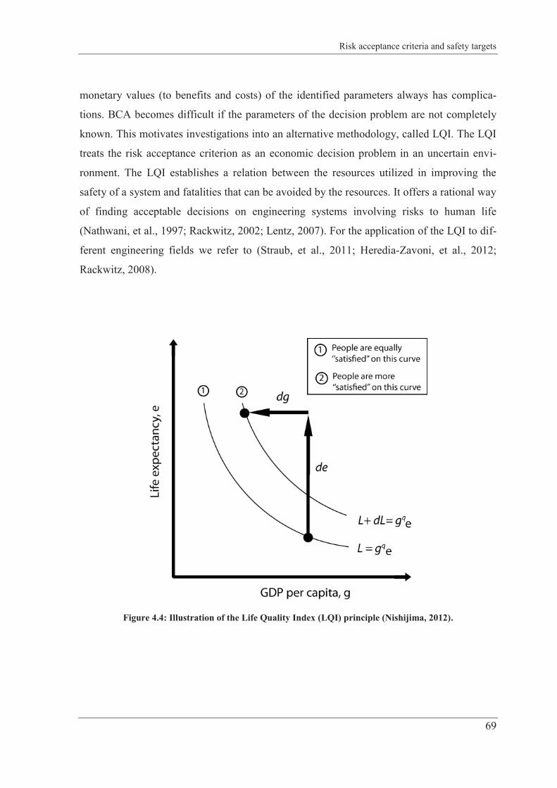
Risk acceptance criteria and safety targets
69
monetary values (to benefits and costs) of the identified parameters always has complica-
tions. BCA becomes difficult if the parameters of the decision problem are not completely
known. This motivates investigations into an alternative methodology, called LQI. The LQI
treats the risk acceptance criterion as an economic decision problem in an uncertain envi-
ronment. The LQI establishes a relation between the resources utilized in improving the
safety of a system and fatalities that can be avoided by the resources. It offers a rational way
of finding acceptable decisions on engineering systems involving risks to human life
(Nathwani, et al., 1997; Rackwitz, 2002; Lentz, 2007). For the application of the LQI to dif-
ferent engineering fields we refer to (Straub, et al., 2011; Heredia-Zavoni, et al., 2012;
Rackwitz, 2008).
Figure 4.4: Illustration of the Life Quality Index (LQI) principle (Nishijima, 2012).
A Bayesian Network Methodology for Railway Risk, Safety and Decision Support
70
The LQI is a combined utility function (illustrated in Figure 4.4), which is based on two so-
cial indicators; life expectancy at birth, and the real GDP. The strong assumption in the LQI
formulation is that people (on average) choose an optimum work-life balance, which is ex-
changeable. In general, persons may substitute work time for work-free time and vice versa
to optimize their total life. For example, in the context of individual risk, one can be willing
to accept additional risk of death or injury in the workplace if he or she gets appropriate ad-
ditional monetary benefits that are appropriate to his or her expected utilities. So, the LQI
can be regarded as a utility function, which reflects the net benefits to society.
In this thesis, we do not discuss the mathematical derivations and details of the LQI, but
show its application to the railway system, which involves risk. As yet, there has been no
any application of the LQI to railway risks.
With few weak assumptions, the formula for LQI (L) can be written as
In the equation above, is life expectancy of the safety technology user, the constant pa-
rameter is a measure of the trade-off between the resources available for consumption and
the value of the time during the (productive or workable) life. depends on the part of life
allocated for economic activities and the Cobb-Douglas parameter for the production
function. accounts for the fact that only a part of the GDP per capita ( is obtained
through work activities and the rest of the GDP is obtained through return investments. is
estimated as follows:
The general acceptance criteria for a small change in the LQI ( ) due to a safety technolo-
gy or measure can be assessed by
(4.1)
(4.2)
Risk acceptance criteria and safety targets
71
Fatalities can be minimized and, consequently, life years can be saved if any suitable safety
technology is introduced in a railway facility, such as at a railway LC. As a result, a change
in life expectancy at society level will be obtained. The (yearly) cost of a safety technol-
ogy is expressed as a reduction in GDP (money spent on a safety related project such as
the installation of an LC barrier). The LQI acceptance criteria implies that the safety tech-
nology is implemented as long as
The (-) with in the equation above refers to the cost of installing a safety technology. In
general, the decision on safety technology has parallel effects on the risk level and income.
For example, safety technology will lead to high average life expectancy and its cost leads
to a decrease in average income . The societal capacity to commit resources (SCCR), also
called societal-willingness-to-pay (SWTP), towards a risk reduction measure is the amount
that society is willing to pay to retain its original level of welfare by following a welfare
change. A safety technology is accepted if the overall life time utility increases or remains
the same. Therefore, the SCCR is the sum received from persons which, following a wel-
fare change, leaves them at their initial level of welfare. The SCCR for a safety technology
is computed as following:
By using the LQI principle, the statistical-value-of-societal life (SVSL) is computed
as (Rackwitz, 2004). It should be mentioned that the SCCR type criterion above
is applied to risk aversion problems where saving the life of some individual member of so-
(4.3)
(4.4)
(4.5)
A Bayesian Network Methodology for Railway Risk, Safety and Decision Support
72
ciety is not identifiable in advance. The mathematical relations above for LQI can be calcu-
lated from widely available and reliable data for many countries (Rackwitz, 2008), especial-
ly, for developed countries where data is easily available. For further details on the mathe-
matical derivations and applications of the LQI approach readers are referred to (Nathwani,
et al., 1997; Rackwitz, 2002; Lentz, 2007; Heredia-Zavoni, et al., 2012) and the references
therein.
4.8 Summary
ALARP, MEM and MGS risk acceptance criteria are widely applied and accepted in rail-
ways. These criteria are used to determine a tolerable level of risk on a railway that can arise
due to any technical failure or natural hazard. In order to create a balance between random
failures and systematic errors, the SIL approach is used on railways. Based on the tolerable
level of the individual or collective risk of fatality, an acceptable level of dangerous failures
per hour can be determined using the SIL approach. Brief definitions of different IMs,
which are useful in answering a number of questions on system risk, safety and reliability,
are given. IMs can be utilized to identify and rank the important components in railways.
LQI is an economic based risk acceptance criterion when human life is at risk. It creates a
relation between the resources utilized in improving the safety of an engineering system and
the potential fatalities that can be avoided by the investment.
CHAPTER 5: APPLICATION OF BAYESIAN NETWORKS TO COM-PLEX RAILWAYS: A STUDY ON DE-RAILMENT ACCIDENTS
5.1 Introduction
This chapter presents an example of a train derailment due to SPAD, which can occur in
railways when train passes a red signal. A number of failures and factors can cause SPAD.
For example, SPAD can be caused by faulty brakes, high train speed, defective signals and
train drivers wrongly reading and responding to cautionary signals. To prevent SPAD, mod-
ern railways have automatic signalling and train protection and warning systems. The auto-
matic signalling provides trains the possibility to proceed further and ensure an adequate
distance between the trains to avoid accidents. The train protection and warning systems
further ensure safe train movement by automatically applying the brakes if the train speed is
higher than the permission. The SPAD event can further lead to adverse events such as train
derailment. For instance, a train derailment occurs if the turnout/point ahead is not set in the
overlap length3 or the train speed is high, and there is a sharp curve in the overlap length.
The train derailment can cause a number of consequences to people, infrastructure, opera-
tional processes and environment. The severity of these consequences depends on so-called
barriers and neutralizing factors that may exist in between the top event and the conse-
quences. There exist a number of dependencies between the causes of the train derailment.
For example, high train speed is a common cause failure; slip and failure towards brake ap-
plication are disjoint events; failure dependency exists between TPWS and driver errors;
driver errors are time dependent and there is functional uncertainty for derailment condi-
3 Overlap length is provided by positioning the signal some way before (say 200 meters) the entrance to the section it is protecting.
A Bayesian Network Methodology for Railway Risk, Safety and Decision Support
74
tions. Additionally, accident scenarios (originated from the train derailment leading to con-
sequences) have dependencies due to common barriers and neutralizing factors.
5.2 Fault Tree Analysis for train derailment due to SPAD
A cause consequence analysis, also called safety risk model (SRM) or bow-tie model, which
is explained in section 2.7, is shown in Figure 5.1 for train derailment accidents. The causes
and the consequences of the Train derailment event are modelled using FTA and ETA, re-
spectively. The lower part of the TE in Figure 5.1 is FTA (Mahboob, et al., 2012(d)).
The possible scenarios leading to the TE are shown in the FTA. For example, intermediate
event SPAD will occur when Train is approaching a red signal, and there are (1) combined
failures of TPWS and Driver errors, or (2) Slip due to poor adhesion between the rail and
wheels. The TE Train derailment can occur when the SPAD is followed by a (1) a Turn-
out/point with prevented route or (2) a Curve in track alignment as well as High train speed.
It is assumed that the driver has no information on a slippery track conditions. Therefore,
the driver is unable to take care of slip related aspects during brake application. The basic
events of the scenarios leading to the top event and their frequencies (for illustration only)
are summarized in Table 5.1. It is to mention that only Fixed Unavailability Values (FUV)
and Failure Frequencies (FF) are used for basic events in the FTA. The FUV and FF are
utilized to represent the probability of failure on demand and simple event probabilities. For
example, one driver failure per 1000 brakes application demands, 15 out of 100 trains ex-
ceed the speed limit while passing a signal, one failure per hundred thousand demands of
TPWS, and every 10th turnout/point is not set in advance.
In general, the probability of TE ( ) in the FT is computed as the function of the min-
imal cut sets by using inclusion and exclusion principle (see Eq. (2.1)) or de Morgan’s law.
The de Morgan’s law for the ‘’Union of Events’’ is written as4
4 The identity only holds for statistically independent events.
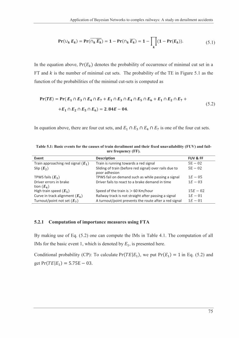
Application of Bayesian Networks to complex railways: A study on derailment accidents
75
In the equation above, denotes the probability of occurrence of minimal cut set in a
FT and is the number of minimal cut sets. The probability of the TE in Figure 5.1 as the
function of the probabilities of the minimal cut-sets is computed as
In equation above, there are four cut sets, and is one of the four cut sets.
Table 5.1: Basic events for the causes of train derailment and their fixed unavailability (FUV) and fail-
ure frequency (FF).
Event Description FUV & FF Train approaching red signal Train is running towards a red signal Slip Sliding of train (before red signal) over rails due to
poor adhesion TPWS fails TPWS fail on demand such as while passing a signal Driver errors in brake tion
Driver fails to react to a brake demand in time
High train speed Speed of the train is 60 Km/hour Curve in track alignment Railway track is not straight after passing a signal Turnout/point not set A turnout/point prevents the route after a red signal
5.2.1 Computation of importance measures using FTA
By making use of Eq. (5.2) one can compute the IMs in Table 4.1. The computation of all
IMs for the basic event 1, which is denoted by , is presented here.
Conditional probability (CP): To calculate , we put in Eq. (5.2) and
get
(5.1)
(5.2)
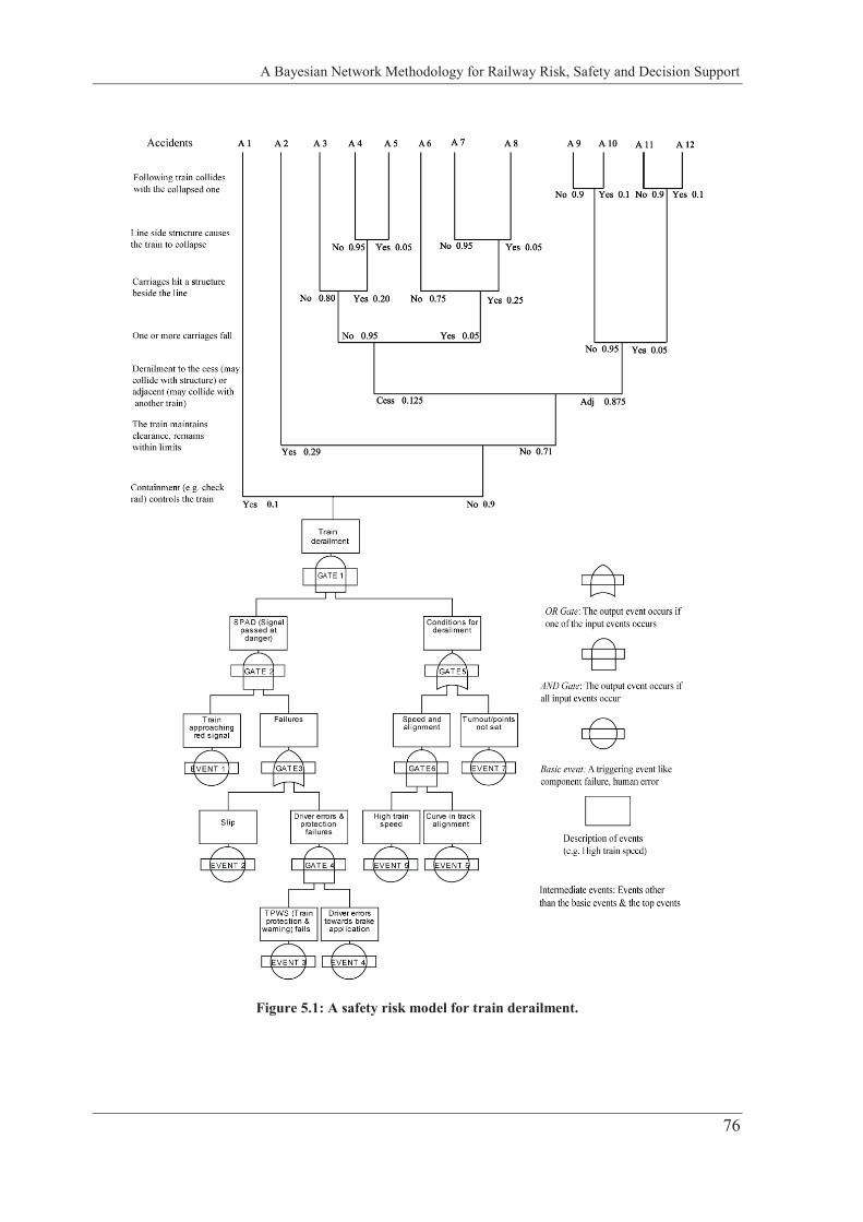
A Bayesian Network Methodology for Railway Risk, Safety and Decision Support
76
Figure 5.1: A safety risk model for train derailment.
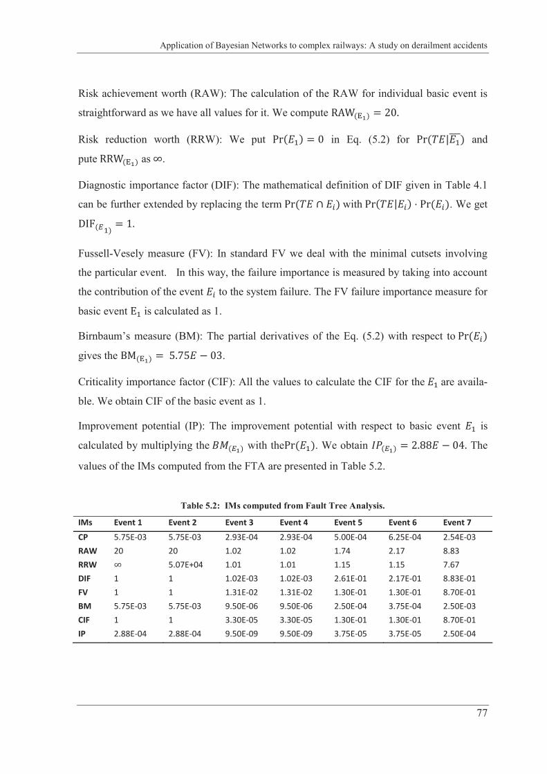
Application of Bayesian Networks to complex railways: A study on derailment accidents
77
Risk achievement worth (RAW): The calculation of the RAW for individual basic event is
straightforward as we have all values for it. We compute
Risk reduction worth (RRW): We put in Eq. (5.2) for and
pute as .
Diagnostic importance factor (DIF): The mathematical definition of DIF given in Table 4.1
can be further extended by replacing the term with . We get
Fussell-Vesely measure (FV): In standard FV we deal with the minimal cutsets involving
the particular event. In this way, the failure importance is measured by taking into account
the contribution of the event to the system failure. The FV failure importance measure for
basic event is calculated as 1.
Birnbaum’s measure (BM): The partial derivatives of the Eq. (5.2) with respect to
gives the .
Criticality importance factor (CIF): All the values to calculate the CIF for the are availa-
ble. We obtain CIF of the basic event as 1.
Improvement potential (IP): The improvement potential with respect to basic event is
calculated by multiplying the with the . We obtain The
values of the IMs computed from the FTA are presented in Table 5.2.
Table 5.2: IMs computed from Fault Tree Analysis.
IMs Event 1 Event 2 Event 3 Event 4 Event 5 Event 6 Event 7
CP 5.75E-03 5.75E-03 2.93E-04 2.93E-04 5.00E-04 6.25E-04 2.54E-03 RAW 20 20 1.02 1.02 1.74 2.17 8.83 RRW 5.07E+04 1.01 1.01 1.15 1.15 7.67 DIF 1 1 1.02E-03 1.02E-03 2.61E-01 2.17E-01 8.83E-01 FV 1 1 1.31E-02 1.31E-02 1.30E-01 1.30E-01 8.70E-01 BM 5.75E-03 5.75E-03 9.50E-06 9.50E-06 2.50E-04 3.75E-04 2.50E-03 CIF 1 1 3.30E-05 3.30E-05 1.30E-01 1.30E-01 8.70E-01 IP 2.88E-04 2.88E-04 9.50E-09 9.50E-09 3.75E-05 3.75E-05 2.50E-04
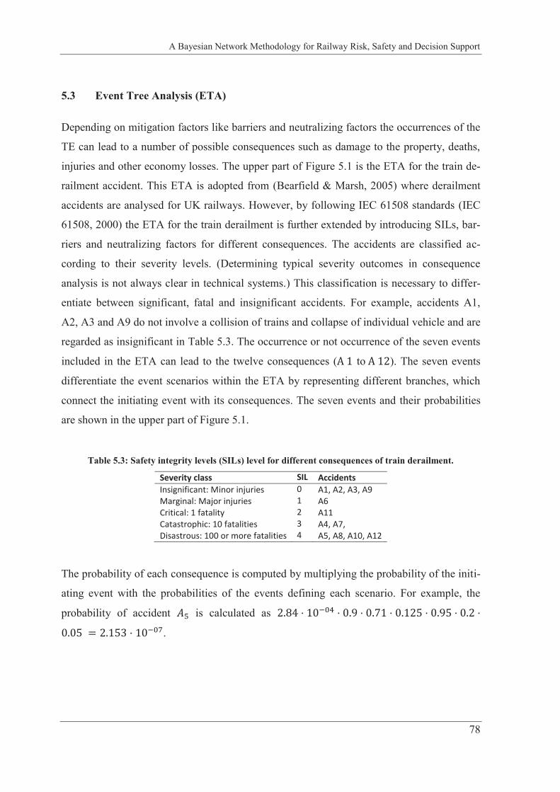
A Bayesian Network Methodology for Railway Risk, Safety and Decision Support
78
5.3 Event Tree Analysis (ETA)
Depending on mitigation factors like barriers and neutralizing factors the occurrences of the
TE can lead to a number of possible consequences such as damage to the property, deaths,
injuries and other economy losses. The upper part of Figure 5.1 is the ETA for the train de-
railment accident. This ETA is adopted from (Bearfield & Marsh, 2005) where derailment
accidents are analysed for UK railways. However, by following IEC 61508 standards (IEC
61508, 2000) the ETA for the train derailment is further extended by introducing SILs, bar-
riers and neutralizing factors for different consequences. The accidents are classified ac-
cording to their severity levels. (Determining typical severity outcomes in consequence
analysis is not always clear in technical systems.) This classification is necessary to differ-
entiate between significant, fatal and insignificant accidents. For example, accidents A1,
A2, A3 and A9 do not involve a collision of trains and collapse of individual vehicle and are
regarded as insignificant in Table 5.3. The occurrence or not occurrence of the seven events
included in the ETA can lead to the twelve consequences ( to ). The seven events
differentiate the event scenarios within the ETA by representing different branches, which
connect the initiating event with its consequences. The seven events and their probabilities
are shown in the upper part of Figure 5.1.
Table 5.3: Safety integrity levels (SILs) level for different consequences of train derailment.
Severity class SIL Accidents Insignificant: Minor injuries 0 A1, A2, A3, A9 Marginal: Major injuries 1 A6 Critical: 1 fatality 2 A11 Catastrophic: 10 fatalities 3 A4, A7, Disastrous: 100 or more fatalities 4 A5, A8, A10, A12
The probability of each consequence is computed by multiplying the probability of the initi-
ating event with the probabilities of the events defining each scenario. For example, the
probability of accident is calculated as
.
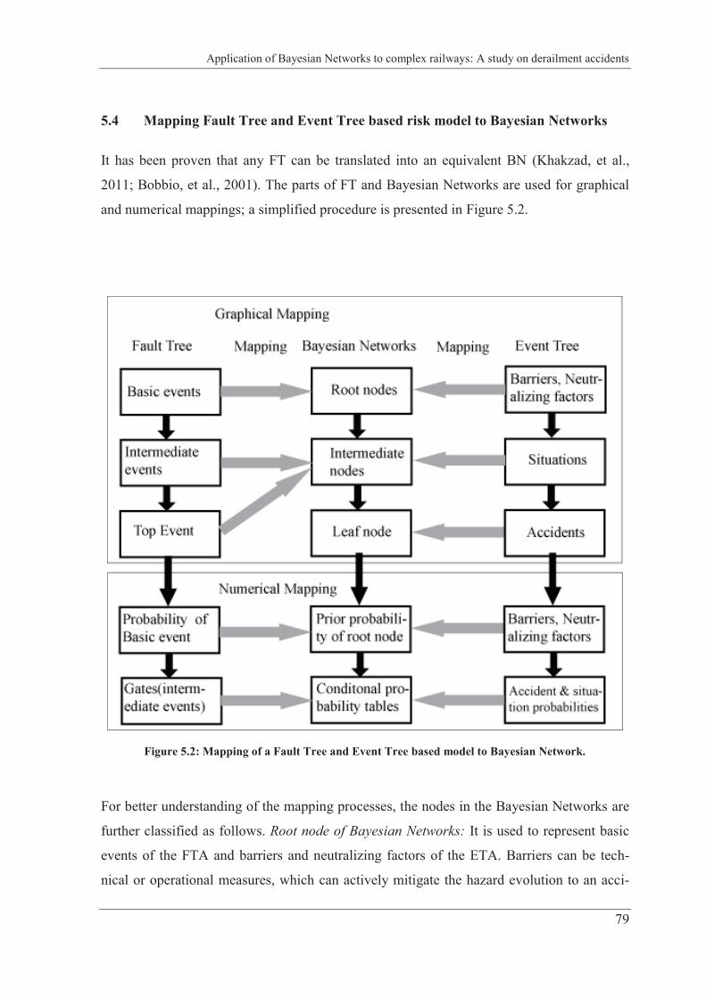
Application of Bayesian Networks to complex railways: A study on derailment accidents
79
5.4 Mapping Fault Tree and Event Tree based risk model to Bayesian Networks
It has been proven that any FT can be translated into an equivalent BN (Khakzad, et al.,
2011; Bobbio, et al., 2001). The parts of FT and Bayesian Networks are used for graphical
and numerical mappings; a simplified procedure is presented in Figure 5.2.
Figure 5.2: Mapping of a Fault Tree and Event Tree based model to Bayesian Network.
For better understanding of the mapping processes, the nodes in the Bayesian Networks are
further classified as follows. Root node of Bayesian Networks: It is used to represent basic
events of the FTA and barriers and neutralizing factors of the ETA. Barriers can be tech-
nical or operational measures, which can actively mitigate the hazard evolution to an acci-
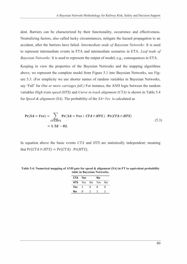
A Bayesian Network Methodology for Railway Risk, Safety and Decision Support
80
dent. Barriers can be characterized by their functionality, occurrence and effectiveness.
Neutralizing factors, also called lucky circumstances, mitigate the hazard propagation to an
accident, after the barriers have failed. Intermediate node of Bayesian Networks: It is used
to represent intermediate events in FTA and intermediate scenarios in ETA. Leaf node of
Bayesian Networks: It is used to represent the output of model; e.g., consequences in ETA.
Keeping in view the properties of the Bayesian Networks and the mapping algorithms
above, we represent the complete model from Figure 5.1 into Bayesian Networks, see Fig-
ure 5.3. (For simplicity we use shorter names of random variables in Bayesian Networks,
say ‘Fall’ for One or more carriages fall.) For instance, the AND logic between the random
variables High train speed (HTS) and Curve in track alignment (CTA) is shown in Table 5.4
for Speed & alignment (SA). The probability of the SA=Yes is calculated as
In equation above the basic events CTA and HTS are statistically independent; meaning
that .
Table 5.4: Numerical mapping of AND gate for speed & alignment (SA) in FT to equivalent probability table in Bayesian Networks.
CTA Yes No HTS Yes No Yes No Yes 1 0 0 0 No 0 1 1 1
(5.3)
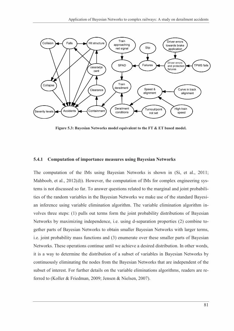
Application of Bayesian Networks to complex railways: A study on derailment accidents
81
Figure 5.3: Bayesian Networks model equivalent to the FT & ET based model.
5.4.1 Computation of importance measures using Bayesian Networks
The computation of the IMs using Bayesian Networks is shown in (Si, et al., 2011;
Mahboob, et al., 2012(d)). However, the computation of IMs for complex engineering sys-
tems is not discussed so far. To answer questions related to the marginal and joint probabili-
ties of the random variables in the Bayesian Networks we make use of the standard Bayesi-
an inference using variable elimination algorithm. The variable elimination algorithm in-
volves three steps: (1) pulls out terms form the joint probability distributions of Bayesian
Networks by maximizing independence, i.e. using d-separation properties (2) combine to-
gether parts of Bayesian Networks to obtain smaller Bayesian Networks with larger terms,
i.e. joint probability mass functions and (3) enumerate over these smaller parts of Bayesian
Networks. These operations continue until we achieve a desired distribution. In other words,
it is a way to determine the distribution of a subset of variables in Bayesian Networks by
continuously eliminating the nodes from the Bayesian Networks that are independent of the
subset of interest. For further details on the variable eliminations algorithms, readers are re-
ferred to (Koller & Friedman, 2009; Jensen & Nielsen, 2007).
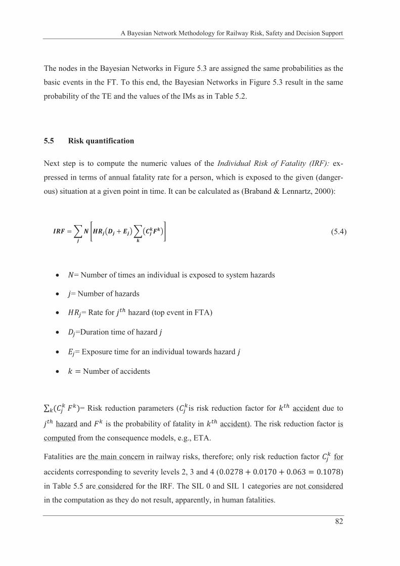
A Bayesian Network Methodology for Railway Risk, Safety and Decision Support
82
The nodes in the Bayesian Networks in Figure 5.3 are assigned the same probabilities as the
basic events in the FT. To this end, the Bayesian Networks in Figure 5.3 result in the same
probability of the TE and the values of the IMs as in Table 5.2.
5.5 Risk quantification
Next step is to compute the numeric values of the Individual Risk of Fatality (IRF): ex-
pressed in terms of annual fatality rate for a person, which is exposed to the given (danger-
ous) situation at a given point in time. It can be calculated as (Braband & Lennartz, 2000):
= Number of times an individual is exposed to system hazards
= Number of hazards
= Rate for hazard (top event in FTA)
=Duration time of hazard
= Exposure time for an individual towards hazard
Number of accidents
= Risk reduction parameters ( is risk reduction factor for accident due to
hazard and is the probability of fatality in accident). The risk reduction factor is
computed from the consequence models, e.g., ETA.
Fatalities are the main concern in railway risks, therefore; only risk reduction factor for
accidents corresponding to severity levels 2, 3 and 4 ( )
in Table 5.5 are considered for the IRF. The SIL 0 and SIL 1 categories are not considered
in the computation as they do not result, apparently, in human fatalities.
(5.4)
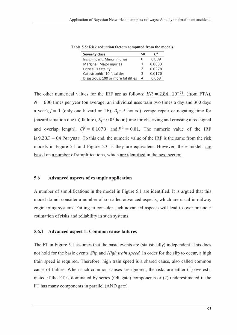
Application of Bayesian Networks to complex railways: A study on derailment accidents
83
Table 5.5: Risk reduction factors computed from the models.
Severity class SIL Insignificant: Minor injuries 0 Marginal: Major injuries 1 Critical: 1 fatality 2 Catastrophic: 10 fatalities 3 Disastrous: 100 or more fatalities 4
The other numerical values for the IRF are as follows: (from FTA),
times per year (on average, an individual uses train two times a day and 300 days
a year), (only one hazard or TE), = 5 hours (average repair or negating time for
(hazard situation due to) failure), = 0.05 hour (time for observing and crossing a red signal
and overlap length), and . The numeric value of the IRF
is . To this end, the numeric value of the IRF is the same from the risk
models in Figure 5.1 and Figure 5.3 as they are equivalent. However, these models are
based on a number of simplifications, which are identified in the next section.
5.6 Advanced aspects of example application
A number of simplifications in the model in Figure 5.1 are identified. It is argued that this
model do not consider a number of so-called advanced aspects, which are usual in railway
engineering systems. Failing to consider such advanced aspects will lead to over or under
estimation of risks and reliability in such systems.
5.6.1 Advanced aspect 1: Common cause failures
The FT in Figure 5.1 assumes that the basic events are (statistically) independent. This does
not hold for the basic events Slip and High train speed. In order for the slip to occur, a high
train speed is required. Therefore, high train speed is a shared cause, also called common
cause of failure. When such common causes are ignored, the risks are either (1) overesti-
mated if the FT is dominated by series (OR gate) components or (2) underestimated if the
FT has many components in parallel (AND gate).
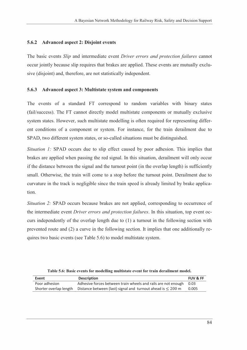
A Bayesian Network Methodology for Railway Risk, Safety and Decision Support
84
5.6.2 Advanced aspect 2: Disjoint events
The basic events Slip and intermediate event Driver errors and protection failures cannot
occur jointly because slip requires that brakes are applied. These events are mutually exclu-
sive (disjoint) and, therefore, are not statistically independent.
5.6.3 Advanced aspect 3: Multistate system and components
The events of a standard FT correspond to random variables with binary states
(fail/success). The FT cannot directly model multistate components or mutually exclusive
system states. However, such multistate modelling is often required for representing differ-
ent conditions of a component or system. For instance, for the train derailment due to
SPAD, two different system states, or so-called situations must be distinguished.
Situation 1: SPAD occurs due to slip effect caused by poor adhesion. This implies that
brakes are applied when passing the red signal. In this situation, derailment will only occur
if the distance between the signal and the turnout point (in the overlap length) is sufficiently
small. Otherwise, the train will come to a stop before the turnout point. Derailment due to
curvature in the track is negligible since the train speed is already limited by brake applica-
tion.
Situation 2: SPAD occurs because brakes are not applied, corresponding to occurrence of
the intermediate event Driver errors and protection failures. In this situation, top event oc-
curs independently of the overlap length due to (1) a turnout in the following section with
prevented route and (2) a curve in the following section. It implies that one additionally re-
quires two basic events (see Table 5.6) to model multistate system.
Table 5.6: Basic events for modelling multistate event for train derailment model.
Event Description FUV & FF Poor adhesion Adhesive forces between train wheels and rails are not enough 0.03Shorter overlap length Distance between (last) signal and turnout ahead is m 0.005
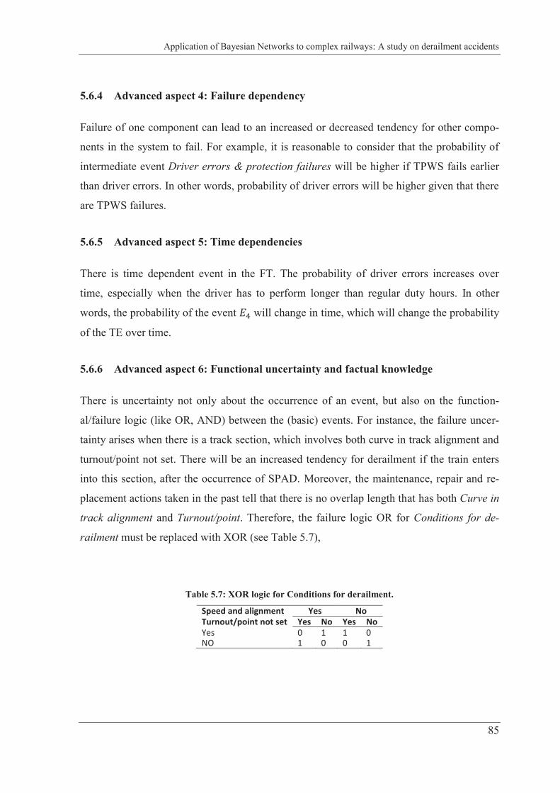
Application of Bayesian Networks to complex railways: A study on derailment accidents
85
5.6.4 Advanced aspect 4: Failure dependency
Failure of one component can lead to an increased or decreased tendency for other compo-
nents in the system to fail. For example, it is reasonable to consider that the probability of
intermediate event Driver errors & protection failures will be higher if TPWS fails earlier
than driver errors. In other words, probability of driver errors will be higher given that there
are TPWS failures.
5.6.5 Advanced aspect 5: Time dependencies
There is time dependent event in the FT. The probability of driver errors increases over
time, especially when the driver has to perform longer than regular duty hours. In other
words, the probability of the event will change in time, which will change the probability
of the TE over time.
5.6.6 Advanced aspect 6: Functional uncertainty and factual knowledge
There is uncertainty not only about the occurrence of an event, but also on the function-
al/failure logic (like OR, AND) between the (basic) events. For instance, the failure uncer-
tainty arises when there is a track section, which involves both curve in track alignment and
turnout/point not set. There will be an increased tendency for derailment if the train enters
into this section, after the occurrence of SPAD. Moreover, the maintenance, repair and re-
placement actions taken in the past tell that there is no overlap length that has both Curve in
track alignment and Turnout/point. Therefore, the failure logic OR for Conditions for de-
railment must be replaced with XOR (see Table 5.7),
Table 5.7: XOR logic for Conditions for derailment.
Speed and alignment Yes No Turnout/point not set Yes No Yes No Yes 0 1 1 0 NO 1 0 0 1
A Bayesian Network Methodology for Railway Risk, Safety and Decision Support
86
5.6.7 Advanced aspect 7: Uncertainty in expert knowledge
Where there is not enough historical data to quantify the risks, experts in the field are used
to estimate the probability of occurrence of particular events. Sometime, experts do not
agree on the probability of occurrence of an event. For example, two experts have different
believes on the probability of Curve in track alignment that will lead to the TE.
5.6.8 Advanced aspect 8: Simplifications and dependencies in Event Tree Analysis
The ETA in Figure 5.1 simplifies event scenarios leading to the consequences, thus fails to
include a number of barriers and neutralizing factors. A detailed presentation of barriers and
neutralizing factors in the field of railways is given in (Puettner & Geisler, 2008). For the
purpose of the exemplification of the use of Bayesian Networks in the calculation of risks in
the railways, only the following barriers and neutralizing factors are considered here.
Barrier 1- Human intervention to avoid an accident: For instance, driver (staff, passengers
or third person) observes the situation properly and acts accordingly.
Barrier 2- There is an independent (technical protection) device in the system that has to
intervene in case of an accident. For example, slip sidings are provided if the gradient fall-
ing away from the signal or station is steeper.
Neutralizing factor 1- Operational environment: It could be unusually low or no trains on
the railway network and passengers in the trains. This could also specify characteristics of
infrastructure in the environment such as bridge and tunnels. For example, accident close to
bridge or in a tunnel can lead to higher consequences.
Neutralizing factor 2- Human exposure and attention: For example, no exposure of person
in hazardous area or human is attentive in case of a hazardous situation.
Depending on the system characteristics, there could be some neutralizing factors and barri-
ers in the ET that are equally valid for the FT. In other words, there are neutralizing factors
and barriers that can prevent both hazard occurrence and its propagation. However, depend-
encies among neutralizing factors and barriers are not considered here. Moreover, the prior
probabilities of every single neutralizing factor and barrier are assumed to be 0.1.
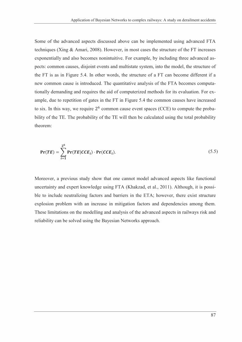
Application of Bayesian Networks to complex railways: A study on derailment accidents
87
Some of the advanced aspects discussed above can be implemented using advanced FTA
techniques (Xing & Amari, 2008). However, in most cases the structure of the FT increases
exponentially and also becomes nonintuitive. For example, by including three advanced as-
pects: common causes, disjoint events and multistate system, into the model, the structure of
the FT is as in Figure 5.4. In other words, the structure of a FT can become different if a
new common cause is introduced. The quantitative analysis of the FTA becomes computa-
tionally demanding and requires the aid of computerized methods for its evaluation. For ex-
ample, due to repetition of gates in the FT in Figure 5.4 the common causes have increased
to six. In this way, we require common cause event spaces (CCE) to compute the proba-
bility of the TE. The probability of the TE will then be calculated using the total probability
theorem:
Moreover, a previous study show that one cannot model advanced aspects like functional
uncertainty and expert knowledge using FTA (Khakzad, et al., 2011). Although, it is possi-
ble to include neutralizing factors and barriers in the ETA; however, there exist structure
explosion problem with an increase in mitigation factors and dependencies among them.
These limitations on the modelling and analysis of the advanced aspects in railways risk and
reliability can be solved using the Bayesian Networks approach.
(5.5)
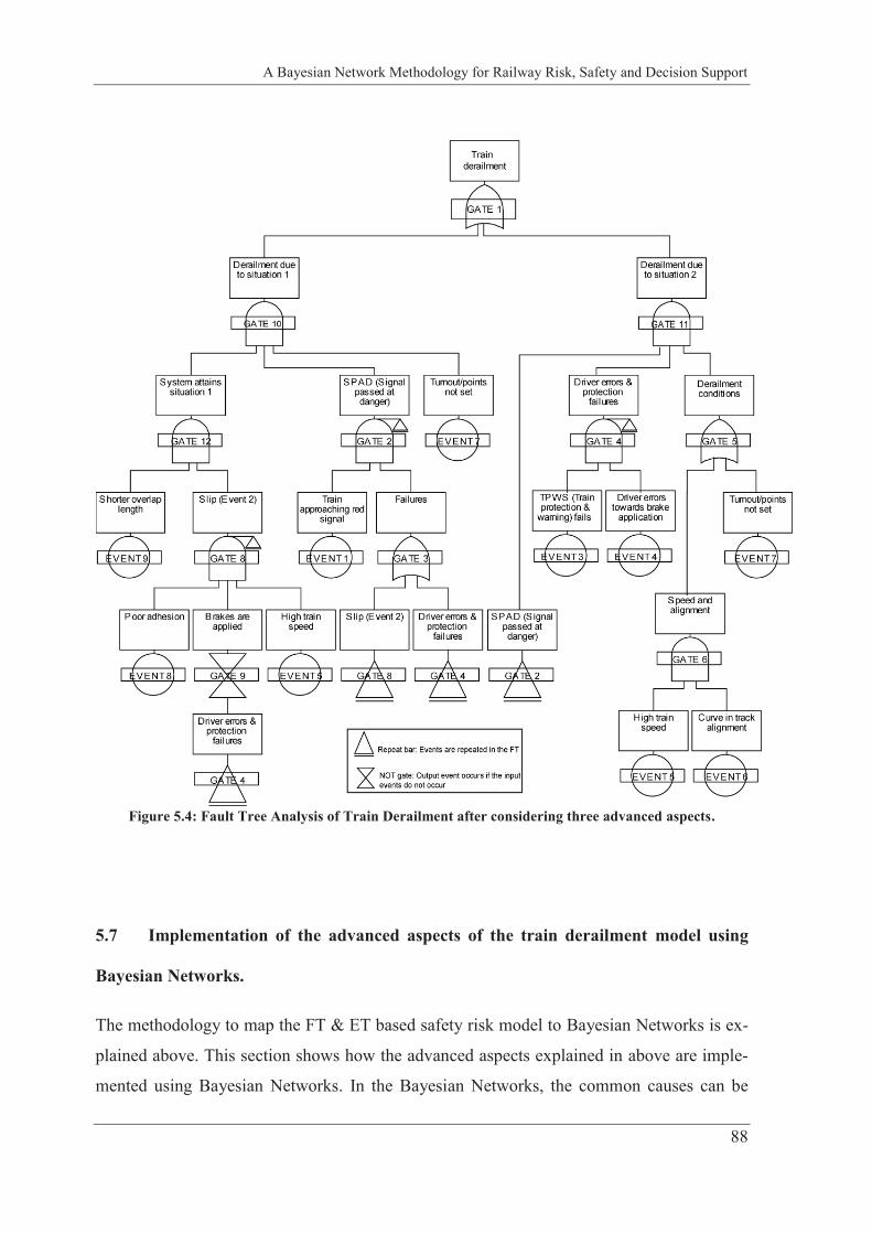
A Bayesian Network Methodology for Railway Risk, Safety and Decision Support
88
Figure 5.4: Fault Tree Analysis of Train Derailment after considering three advanced aspects.
5.7 Implementation of the advanced aspects of the train derailment model using
Bayesian Networks.
The methodology to map the FT & ET based safety risk model to Bayesian Networks is ex-
plained above. This section shows how the advanced aspects explained in above are imple-
mented using Bayesian Networks. In the Bayesian Networks, the common causes can be
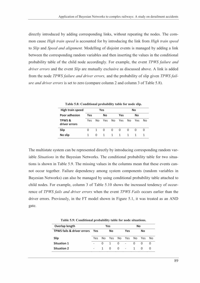
Application of Bayesian Networks to complex railways: A study on derailment accidents
89
directly introduced by adding corresponding links, without repeating the nodes. The com-
mon cause High train speed is accounted for by introducing the link from High train speed
to Slip and Speed and alignment. Modelling of disjoint events is managed by adding a link
between the corresponding random variables and then inserting the values in the conditional
probability table of the child node accordingly. For example, the event TPWS failure and
driver errors and the event Slip are mutually exclusive as discussed above. A link is added
from the node TPWS failure and driver errors, and the probability of slip given TPWS fail-
ure and driver errors is set to zero (compare column 2 and column 3 of Table 5.8).
Table 5.8: Conditional probability table for node slip.
High train speed Yes No Poor adhesion Yes No Yes No TPWS & driver errors
Yes No Yes No Yes No Yes No
Slip 0 1 0 0 0 0 0 0 No slip 1 0 1 1 1 1 1 1
The multistate system can be represented directly by introducing corresponding random var-
iable Situations in the Bayesian Networks. The conditional probability table for two situa-
tions is shown in Table 5.9. The missing values in the columns mean that these events can-
not occur together. Failure dependency among system components (random variables in
Bayesian Networks) can also be managed by using conditional probability table attached to
child nodes. For example, column 3 of Table 5.10 shows the increased tendency of occur-
rence of TPWS fails and driver errors when the event TPWS Fails occurs earlier than the
driver errors. Previously, in the FT model shown in Figure 5.1, it was treated as an AND
gate.
Table 5.9: Conditional probability table for node situations.
Overlap length Yes No TPWS fails & driver errors Yes No Yes No
Slip Yes No Yes No Yes No Yes No Situation 1 - 0 1 0 - 0 0 0 Situation 2 - 1 0 0 - 1 0 0
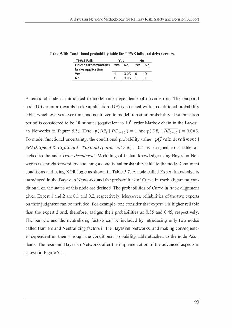
A Bayesian Network Methodology for Railway Risk, Safety and Decision Support
90
Table 5.10: Conditional probability table for TPWS fails and driver errors.
TPWS Fails Yes No Driver errors towards brake application
Yes No Yes No
Yes 1 0.05 0 0 No 0 0.95 1 1
A temporal node is introduced to model time dependence of driver errors. The temporal
node Driver error towards brake application (DE) is attached with a conditional probability
table, which evolves over time and is utilized to model transition probability. The transition
period is considered to be 10 minutes (equivalent to 10th order Markov chain in the Bayesi-
an Networks in Figure 5.5). Here, and .
To model functional uncertainty, the conditional probability value
is assigned to a table at-
tached to the node Train derailment. Modelling of factual knowledge using Bayesian Net-
works is straightforward, by attaching a conditional probability table to the node Derailment
conditions and using XOR logic as shown in Table 5.7. A node called Expert knowledge is
introduced in the Bayesian Networks and the probabilities of Curve in track alignment con-
ditional on the states of this node are defined. The probabilities of Curve in track alignment
given Expert 1 and 2 are 0.1 and 0.2, respectively. Moreover, reliabilities of the two experts
on their judgment can be included. For example, one consider that expert 1 is higher reliable
than the expert 2 and, therefore, assigns their probabilities as 0.55 and 0.45, respectively.
The barriers and the neutralizing factors can be included by introducing only two nodes
called Barriers and Neutralizing factors in the Bayesian Networks, and making consequenc-
es dependent on them through the conditional probability table attached to the node Acci-
dents. The resultant Bayesian Networks after the implementation of the advanced aspects is
shown in Figure 5.5.
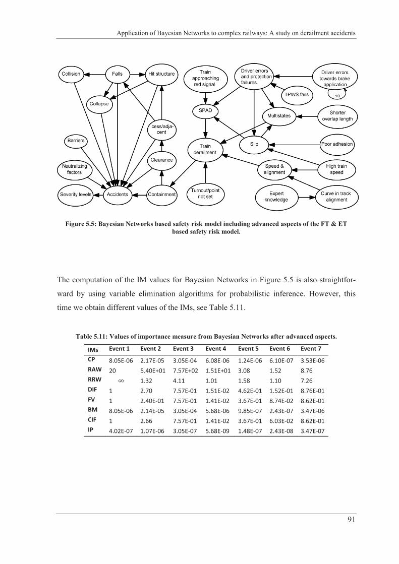
Application of Bayesian Networks to complex railways: A study on derailment accidents
91
Figure 5.5: Bayesian Networks based safety risk model including advanced aspects of the FT & ET based safety risk model.
The computation of the IM values for Bayesian Networks in Figure 5.5 is also straightfor-
ward by using variable elimination algorithms for probabilistic inference. However, this
time we obtain different values of the IMs, see Table 5.11.
Table 5.11: Values of importance measure from Bayesian Networks after advanced aspects.
IMs Event 1 Event 2 Event 3 Event 4 Event 5 Event 6 Event 7
CP 8.05E-06 2.17E-05 3.05E-04 6.08E-06 1.24E-06 6.10E-07 3.53E-06 RAW 20 5.40E+01 7.57E+02 1.51E+01 3.08 1.52 8.76 RRW 1.32 4.11 1.01 1.58 1.10 7.26 DIF 1 2.70 7.57E-01 1.51E-02 4.62E-01 1.52E-01 8.76E-01 FV 1 2.40E-01 7.57E-01 1.41E-02 3.67E-01 8.74E-02 8.62E-01 BM 8.05E-06 2.14E-05 3.05E-04 5.68E-06 9.85E-07 2.43E-07 3.47E-06 CIF 1 2.66 7.57E-01 1.41E-02 3.67E-01 6.03E-02 8.62E-01 IP 4.02E-07 1.07E-06 3.05E-07 5.68E-09 1.48E-07 2.43E-08 3.47E-07
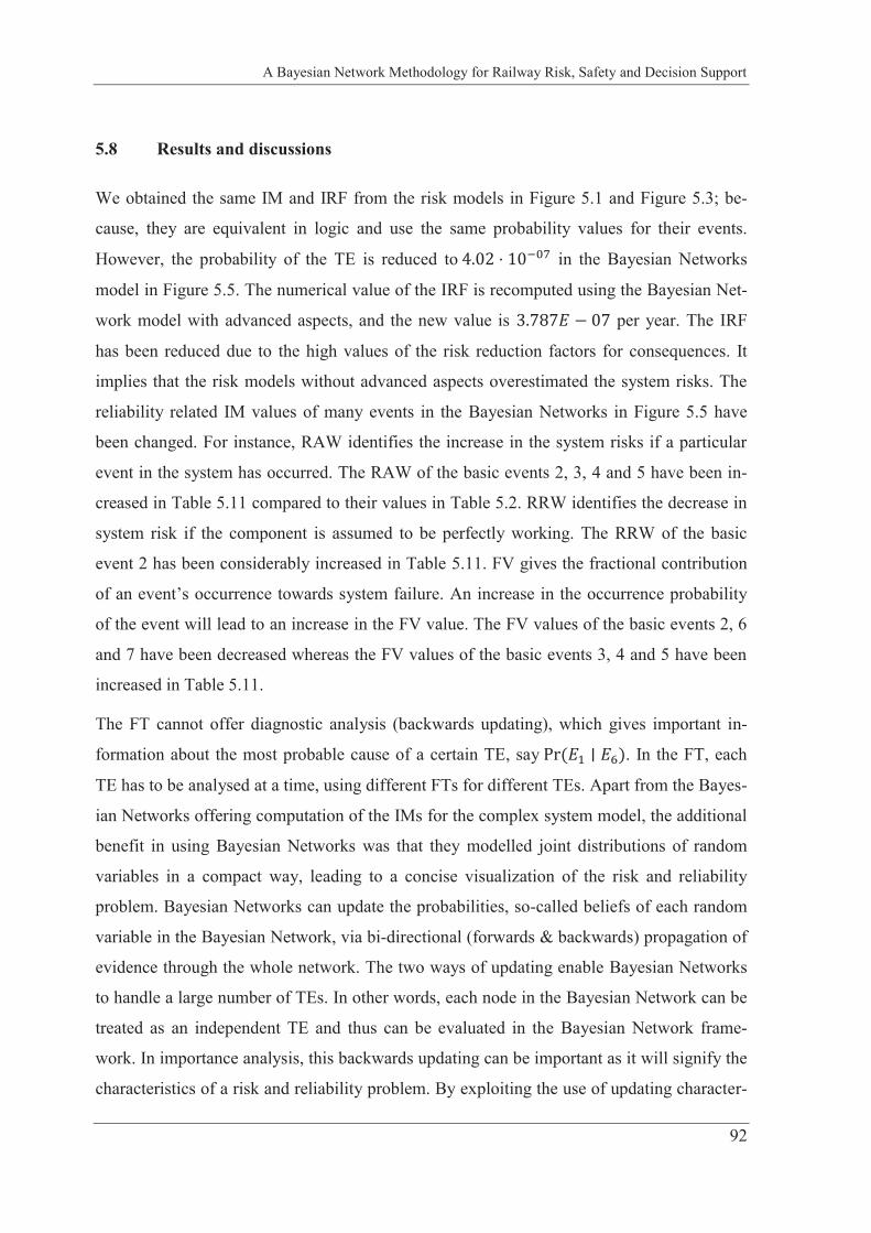
A Bayesian Network Methodology for Railway Risk, Safety and Decision Support
92
5.8 Results and discussions
We obtained the same IM and IRF from the risk models in Figure 5.1 and Figure 5.3; be-
cause, they are equivalent in logic and use the same probability values for their events.
However, the probability of the TE is reduced to in the Bayesian Networks
model in Figure 5.5. The numerical value of the IRF is recomputed using the Bayesian Net-
work model with advanced aspects, and the new value is per year. The IRF
has been reduced due to the high values of the risk reduction factors for consequences. It
implies that the risk models without advanced aspects overestimated the system risks. The
reliability related IM values of many events in the Bayesian Networks in Figure 5.5 have
been changed. For instance, RAW identifies the increase in the system risks if a particular
event in the system has occurred. The RAW of the basic events 2, 3, 4 and 5 have been in-
creased in Table 5.11 compared to their values in Table 5.2. RRW identifies the decrease in
system risk if the component is assumed to be perfectly working. The RRW of the basic
event 2 has been considerably increased in Table 5.11. FV gives the fractional contribution
of an event’s occurrence towards system failure. An increase in the occurrence probability
of the event will lead to an increase in the FV value. The FV values of the basic events 2, 6
and 7 have been decreased whereas the FV values of the basic events 3, 4 and 5 have been
increased in Table 5.11.
The FT cannot offer diagnostic analysis (backwards updating), which gives important in-
formation about the most probable cause of a certain TE, say . In the FT, each
TE has to be analysed at a time, using different FTs for different TEs. Apart from the Bayes-
ian Networks offering computation of the IMs for the complex system model, the additional
benefit in using Bayesian Networks was that they modelled joint distributions of random
variables in a compact way, leading to a concise visualization of the risk and reliability
problem. Bayesian Networks can update the probabilities, so-called beliefs of each random
variable in the Bayesian Network, via bi-directional (forwards & backwards) propagation of
evidence through the whole network. The two ways of updating enable Bayesian Networks
to handle a large number of TEs. In other words, each node in the Bayesian Network can be
treated as an independent TE and thus can be evaluated in the Bayesian Network frame-
work. In importance analysis, this backwards updating can be important as it will signify the
characteristics of a risk and reliability problem. By exploiting the use of updating character-
Application of Bayesian Networks to complex railways: A study on derailment accidents
93
istics of the Bayesian Network, the idea of importance analysis for complex systems can
find new developments and definitions since they can account not only for the components
that are down but also for those that are up at the same time. Moreover, incorporating more
TEs and the eventual interrelated aspects of these TEs, an integrated picture of the risks
characterizing the system risks and reliability can be obtained. Some of the advanced as-
pects mentioned above have been discussed in (Khakzad, et al., 2011) for process facilities,
using Bayesian Networks.
5.9 Summary
A number of advanced aspects and their effects on the quantitative risk and reliability
analysis of a complex railway problem were studied. The implementation of the advanced
aspects using FT, ET, and Bayesian Networks was investigated. The FT and ET based mod-
el has limitations in handling a number of dependencies and uncertainties in complex rail-
ways. In most cases, the structure of the FT increases exponentially and becomes non-
intuitive and computationally demanding. The FT and ET based models are useful for the
risk and reliability problems that have few TEs and few dependencies and uncertainties
among the events leading to the TEs. Moreover, logical visualization of the system architec-
ture is needed, qualitative analysis is part of the risk and reliability analysis and no integra-
tion of new information and (backward) updating are required.
Bayesian Networks offered a suitable probabilistic graphical structure for incorporating a
number of dependencies and uncertainties related to the train derailment problem. The im-
plementation of the advanced aspects was possible using a Bayesian Network and the com-
putation of the IMs for the complex system was straightforward. A Bayesian Networks with
advanced aspects resulted in different values of the fatality risks and the IMs. Bayesian
Networks were able to handle a large number of TEs, intermediate events, uncertainties and
dependencies in complex railways in concise and flexible way.
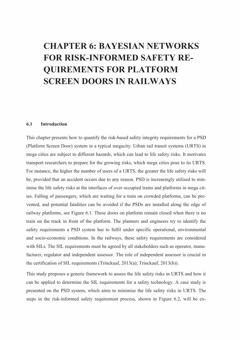
CHAPTER 6: BAYESIAN NETWORKS FOR RISK-INFORMED SAFETY RE-QUIREMENTS FOR PLATFORM SCREEN DOORS IN RAILWAYS
6.1 Introduction
This chapter presents how to quantify the risk-based safety integrity requirements for a PSD
(Platform Screen Door) system in a typical megacity. Urban rail transit systems (URTS) in
mega cities are subject to different hazards, which can lead to life safety risks. It motivates
transport researchers to prepare for the growing risks, which mega cities pose to its URTS.
For instance, the higher the number of users of a URTS, the greater the life safety risks will
be, provided that an accident occurs due to any reason. PSD is increasingly utilised to min-
imise the life safety risks at the interfaces of over occupied trains and platforms in mega cit-
ies. Falling of passengers, which are waiting for a train on crowded platforms, can be pre-
vented, and potential fatalities can be avoided if the PSDs are installed along the edge of
railway platforms, see Figure 6.1. These doors on platform remain closed when there is no
train on the track in front of the platform. The planners and engineers try to identify the
safety requirements a PSD system has to fulfil under specific operational, environmental
and socio-economic conditions. In the railways, these safety requirements are considered
with SILs. The SIL requirements must be agreed by all stakeholders such as operator, manu-
facturer, regulator and independent assessor. The role of independent assessor is crucial in
the certification of SIL requirements (Trinckuaf, 2013(a); Trinckauf, 2013(b)).
This study proposes a generic framework to assess the life safety risks in URTS and how it
can be applied to determine the SIL requirements for a safety technology. A case study is
presented on the PSD system, which aims to minimise the life safety risks in URTS. The
steps in the risk-informed safety requirement process, shown in Figure 6.2, will be ex-
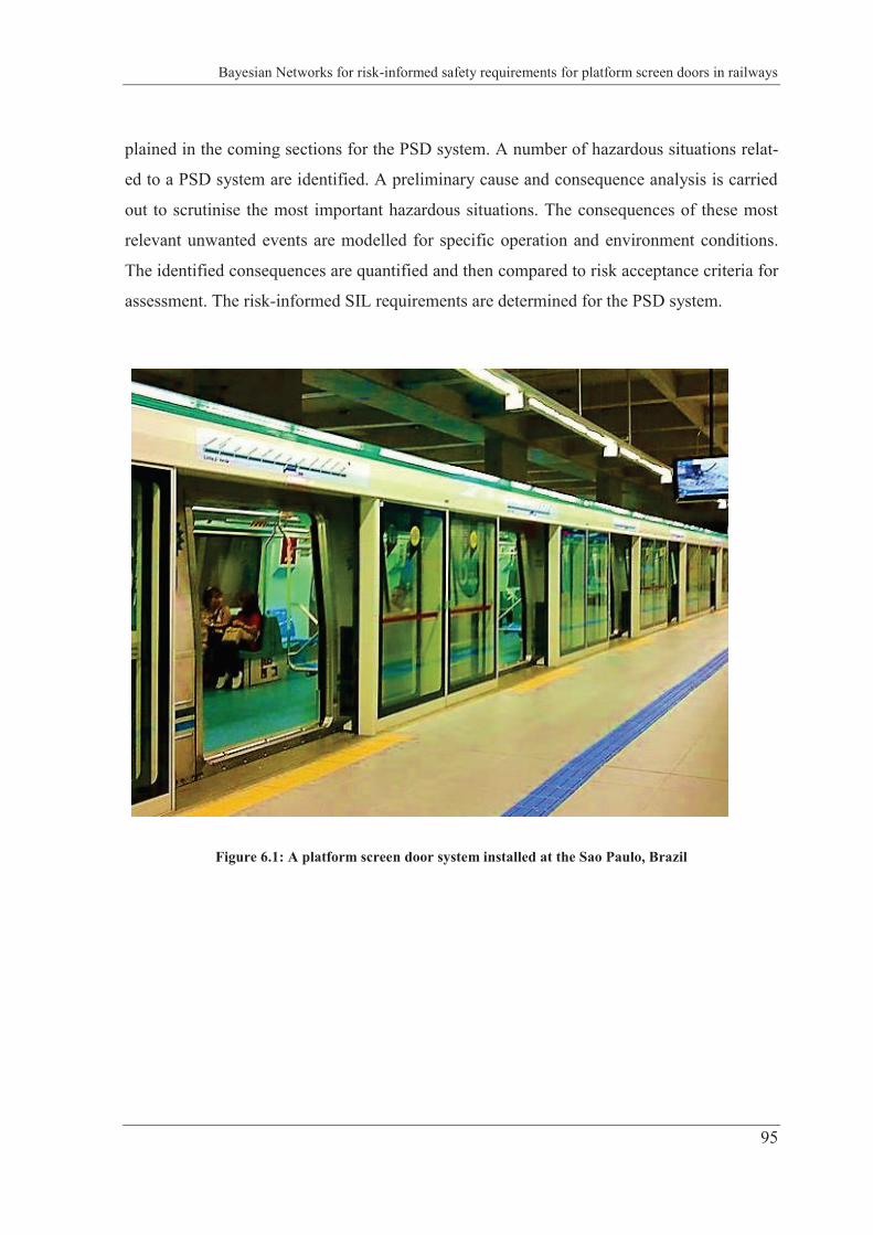
Bayesian Networks for risk-informed safety requirements for platform screen doors in railways
95
plained in the coming sections for the PSD system. A number of hazardous situations relat-
ed to a PSD system are identified. A preliminary cause and consequence analysis is carried
out to scrutinise the most important hazardous situations. The consequences of these most
relevant unwanted events are modelled for specific operation and environment conditions.
The identified consequences are quantified and then compared to risk acceptance criteria for
assessment. The risk-informed SIL requirements are determined for the PSD system.
Figure 6.1: A platform screen door system installed at the Sao Paulo, Brazil
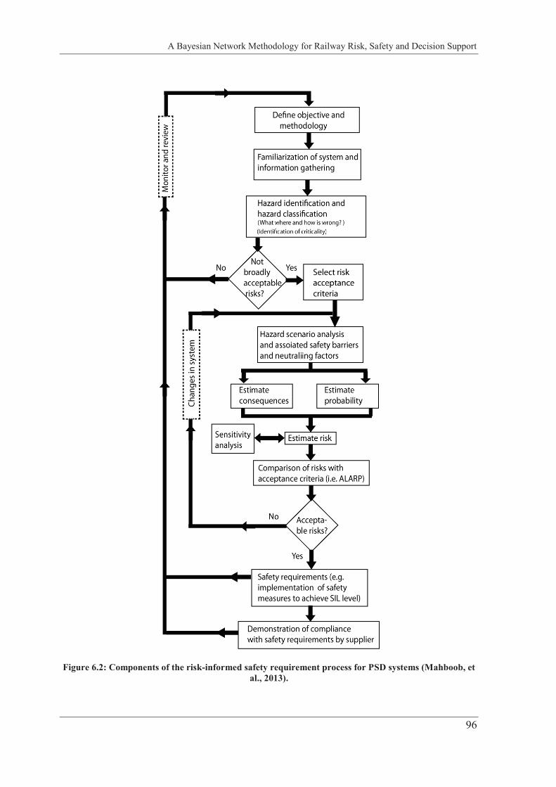
A Bayesian Network Methodology for Railway Risk, Safety and Decision Support
96
Figure 6.2: Components of the risk-informed safety requirement process for PSD systems (Mahboob, et al., 2013).
Bayesian Networks for risk-informed safety requirements for platform screen doors in railways
97
6.2 Components of the risk-informed safety requirement process for Platform
Screen Door system in a mega city
The components of the risk management processes, which are illustrated in Figure 6.2, are
briefly explained in the following sub-sections.
6.2.1 Define objective and methodology
Main objective of the study was to identify and quantify the life safety risks, or so-called
fatality rate, associated to the PSD failures. It was aimed to investigate the acceptability of
such fatality rate for a particular operating condition. The key elements of the basic method-
ologies for determining the SIL for PSD are adopted from the standard probabilistic risk as-
sessment (PRA) processes for the nuclear industry. The PRA are well explained in
(Modarres, 2008; Aven, 2012) and references therein.
6.2.2 Familiarization of system and information gathering
It was important to know about the functioning of technical system and its operational envi-
ronment. Thus, a broad knowledge of typical PSD functioning, physical layout of the plat-
form, critical barriers, passenger demands, operational conditions, emergency safety sys-
tems, and human interactions was gathered. Functional descriptions and planning configura-
tions of PSD installations provided by a manufacturer/supplier were studied. This step re-
quired a comprehensive consultation among supplier, independent assessor and operator of
the URTS.
6.2.3 Hazard identification and hazard classification
A total seventeen possible hazardous situations, which will have potential to affect the hu-
man and system safety, were postulated. A preliminary hazard analysis (PHA) was carried
out with the consultation and support of system manufacturer and operator, see Appendix 1.
It was concluded that not all hazardous situations will lead to severe consequences such fa-
talities. The intention of the PHA was to identify the key hazardous events from the hazard
list. The three most relevant hazardous situations ( corresponding to hazard ID 11,
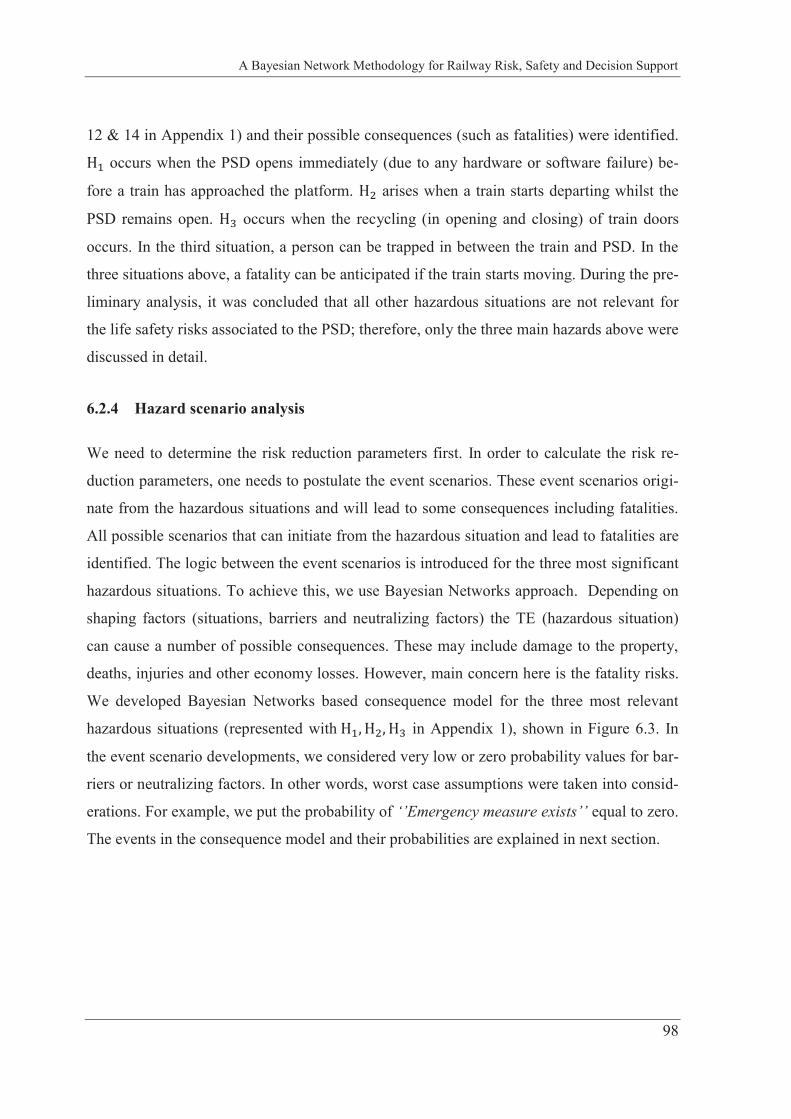
A Bayesian Network Methodology for Railway Risk, Safety and Decision Support
98
12 & 14 in Appendix 1) and their possible consequences (such as fatalities) were identified.
occurs when the PSD opens immediately (due to any hardware or software failure) be-
fore a train has approached the platform. arises when a train starts departing whilst the
PSD remains open. occurs when the recycling (in opening and closing) of train doors
occurs. In the third situation, a person can be trapped in between the train and PSD. In the
three situations above, a fatality can be anticipated if the train starts moving. During the pre-
liminary analysis, it was concluded that all other hazardous situations are not relevant for
the life safety risks associated to the PSD; therefore, only the three main hazards above were
discussed in detail.
6.2.4 Hazard scenario analysis
We need to determine the risk reduction parameters first. In order to calculate the risk re-
duction parameters, one needs to postulate the event scenarios. These event scenarios origi-
nate from the hazardous situations and will lead to some consequences including fatalities.
All possible scenarios that can initiate from the hazardous situation and lead to fatalities are
identified. The logic between the event scenarios is introduced for the three most significant
hazardous situations. To achieve this, we use Bayesian Networks approach. Depending on
shaping factors (situations, barriers and neutralizing factors) the TE (hazardous situation)
can cause a number of possible consequences. These may include damage to the property,
deaths, injuries and other economy losses. However, main concern here is the fatality risks.
We developed Bayesian Networks based consequence model for the three most relevant
hazardous situations (represented with in Appendix 1), shown in Figure 6.3. In
the event scenario developments, we considered very low or zero probability values for bar-
riers or neutralizing factors. In other words, worst case assumptions were taken into consid-
erations. For example, we put the probability of ‘’Emergency measure exists’’ equal to zero.
The events in the consequence model and their probabilities are explained in next section.
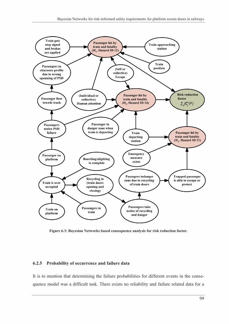
Bayesian Networks for risk-informed safety requirements for platform screen doors in railways
99
Figure 6.3: Bayesian Networks based consequence analysis for risk reduction factor.
6.2.5 Probability of occurrence and failure data
It is to mention that determining the failure probabilities for different events in the conse-
quence model was a difficult task. There exists no reliability and failure related data for a
A Bayesian Network Methodology for Railway Risk, Safety and Decision Support
100
PSD; because, it is a relatively new safety technology. (Unavailability of risk and safety re-
lated data is a usual problem in many engineering risk and safety assessment problems in-
cluding railways.) Therefore, failure frequency and unavailability of the events in the
Bayesian Networks were intensively discussed among supplier, assessor and operator before
their use. How we determine the probability values of the events is explained in the follow-
ing. It is to mention that all probability values are based on peak hour (operational) demands
of a typical URTS in a mega city.
Passengers on platform: Presence of passengers on a platform is necessary for fatality risks,
given that failures in PSD occur. We define probability of passenger on a platform as 1. It is
assumed that there will be always around 200 passengers at one platform side during peak
hour’s operation. With 200 passengers per train per side of the platform, we get
passengers per platform side in a peak hour. (There are 55 trains per hour; it is ex-
plained in the following.) In this way, one platform has peak demand capacity of 22000 pas-
sengers per hour that was according to the operator’s requirement.
Passengers notice PSD failure: There is a possibility that passengers take notice of failure
(that corresponds to premature opening) in PSD and avoid moving towards trackside. It is
mainly based on user’s education, training and experience towards the use of PSD. Here, we
consider that every 4th person takes notice of a PSD failure (probability 0.25). In other
words, one out of four persons observes that the PSD has opened without arrival of the train
and will avoid forward movement.
Passengers flow towards track: It depends on the behaviour/attitude of users. In general,
people standing at platform wait for people in train to leave first. However, there may be
situation (such as mega events) when people at platform do not wait for people in train, but
try to board on the train first. We consider 0.5 probability of passenger flow towards track,
provided that PSD is opened.
Passengers in the danger zone: Here the assumption is made that 50% out of 200 passengers
will not proceed for the very 1st coming train. They intend to take second or later trains. In
this way, 100 passengers are supposed to board on every coming train. Moreover, 80% (out
of 100 passengers that are supposed to take first coming train) will flow towards track and
will remain in clearance profile – probability 0.8. Only 10%
Bayesian Networks for risk-informed safety requirements for platform screen doors in railways
101
will fall on track due to push, negligence and so on. In other words, (based on
above considerations) the probability of a person falling on the track per door is
.
Individual or collective human attention: This includes apprehension of danger from pas-
sengers, emergency and security people available nearby, camera monitoring and so on. The
feeling of danger will raise individual and collective attention. We consider the probability
of attention as 0.9. The high probability implies that there will be a large number of people
available in surroundings during a peak hour or special events.
Self or collective escape: Saving a person in the danger zone (on track or in clearance pro-
file) depends on (1) right individual or collective action and (2) time available for reaction.
The headway (65 sec) is so small, therefore; one can assume that the probability of self or
collective escape is 0.5.
Probability of a train arriving, departing and on the platform: By considering 65 sec of
headway, we can have We assume that a train
takes 36 seconds (3 sec in door opening + 3 sec in door closing + 30 sec in boarding &
alighting) to accomplish the service tasks at a platform. In this way, the probability of a train
on the platform will be .
Here, boarding and alighting of 200 persons per train (in 30 sec) is considered. It means
every door will have to board/alight passengers in 30 sec. (There are 06 vehi-
cles per train and each vehicle has 04 doors.) It is to mention that 200 passengers will be
moving from both sides i.e. from platform to train and train to platform. In this way, total
passenger demand that will be dealt by all trains in one hour becomes
passengers per one side of the platform. For two sided platform, the demand will be 22000
passengers per hour, meeting the specifications requirements from the operator. The proba-
bility that there is no train standing at the platform is . We split this 0.45
probability in the following way.
Probability of train arriving at station = 0.1. According to this probability a train will take
approximately 7 sec from beginning to end of a platform to arrive at a station. Based on 7
sec arrival (and 7 sec for departure) times we get
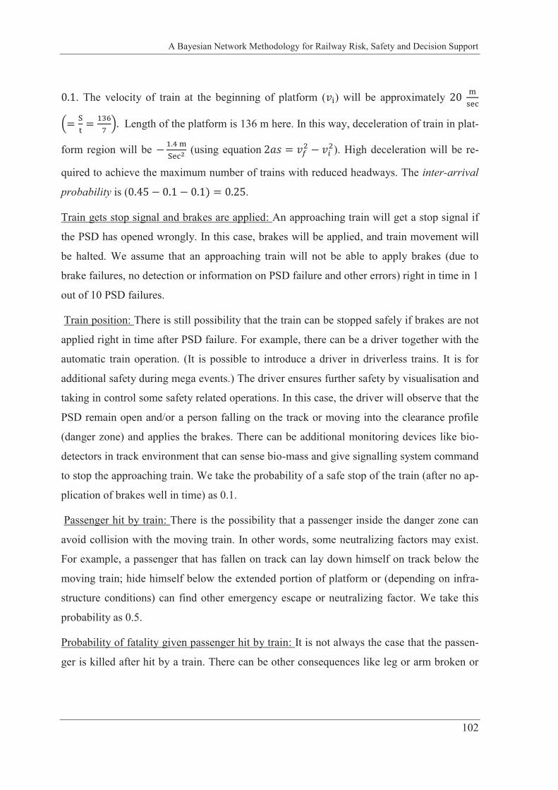
A Bayesian Network Methodology for Railway Risk, Safety and Decision Support
102
. The velocity of train at the beginning of platform ( ) will be approximately
Length of the platform is 136 m here. In this way, deceleration of train in plat-
form region will be (using equation ). High deceleration will be re-
quired to achieve the maximum number of trains with reduced headways. The inter-arrival
probability is ( .
Train gets stop signal and brakes are applied: An approaching train will get a stop signal if
the PSD has opened wrongly. In this case, brakes will be applied, and train movement will
be halted. We assume that an approaching train will not be able to apply brakes (due to
brake failures, no detection or information on PSD failure and other errors) right in time in 1
out of 10 PSD failures.
Train position: There is still possibility that the train can be stopped safely if brakes are not
applied right in time after PSD failure. For example, there can be a driver together with the
automatic train operation. (It is possible to introduce a driver in driverless trains. It is for
additional safety during mega events.) The driver ensures further safety by visualisation and
taking in control some safety related operations. In this case, the driver will observe that the
PSD remain open and/or a person falling on the track or moving into the clearance profile
(danger zone) and applies the brakes. There can be additional monitoring devices like bio-
detectors in track environment that can sense bio-mass and give signalling system command
to stop the approaching train. We take the probability of a safe stop of the train (after no ap-
plication of brakes well in time) as 0.1.
Passenger hit by train: There is the possibility that a passenger inside the danger zone can
avoid collision with the moving train. In other words, some neutralizing factors may exist.
For example, a passenger that has fallen on track can lay down himself on track below the
moving train; hide himself below the extended portion of platform or (depending on infra-
structure conditions) can find other emergency escape or neutralizing factor. We take this
probability as 0.5.
Probability of fatality given passenger hit by train: It is not always the case that the passen-
ger is killed after hit by a train. There can be other consequences like leg or arm broken or
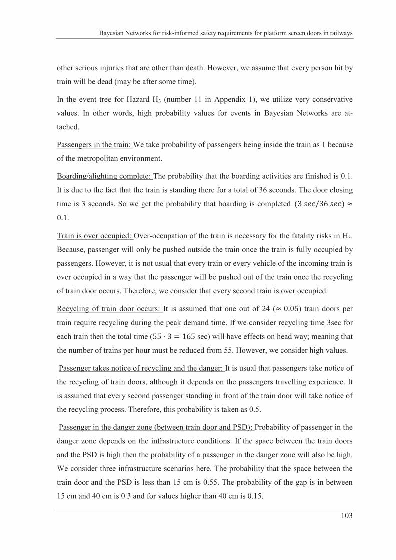
Bayesian Networks for risk-informed safety requirements for platform screen doors in railways
103
other serious injuries that are other than death. However, we assume that every person hit by
train will be dead (may be after some time).
In the event tree for Hazard H3 (number 11 in Appendix 1), we utilize very conservative
values. In other words, high probability values for events in Bayesian Networks are at-
tached.
Passengers in the train: We take probability of passengers being inside the train as 1 because
of the metropolitan environment.
Boarding/alighting complete: The probability that the boarding activities are finished is 0.1.
It is due to the fact that the train is standing there for a total of 36 seconds. The door closing
time is 3 seconds. So we get the probability that boarding is completed
.
Train is over occupied: Over-occupation of the train is necessary for the fatality risks in H3.
Because, passenger will only be pushed outside the train once the train is fully occupied by
passengers. However, it is not usual that every train or every vehicle of the incoming train is
over occupied in a way that the passenger will be pushed out of the train once the recycling
of train door occurs. Therefore, we consider that every second train is over occupied.
Recycling of train door occurs: It is assumed that one out of 24 ( ) train doors per
train require recycling during the peak demand time. If we consider recycling time 3sec for
each train then the total time ( sec) will have effects on head way; meaning that
the number of trains per hour must be reduced from 55. However, we consider high values.
Passenger takes notice of recycling and the danger: It is usual that passengers take notice of
the recycling of train doors, although it depends on the passengers travelling experience. It
is assumed that every second passenger standing in front of the train door will take notice of
the recycling process. Therefore, this probability is taken as 0.5.
Passenger in the danger zone (between train door and PSD): Probability of passenger in the
danger zone depends on the infrastructure conditions. If the space between the train doors
and the PSD is high then the probability of a passenger in the danger zone will also be high.
We consider three infrastructure scenarios here. The probability that the space between the
train door and the PSD is less than 15 cm is 0.55. The probability of the gap is in between
15 cm and 40 cm is 0.3 and for values higher than 40 cm is 0.15.
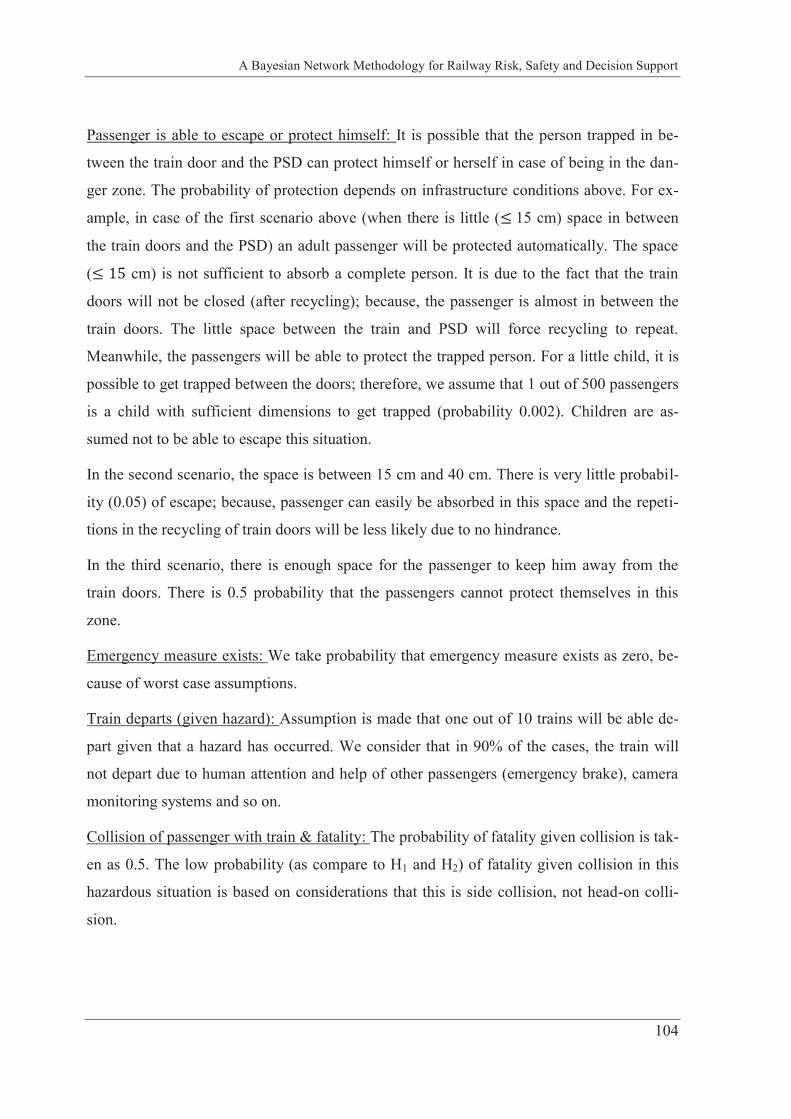
A Bayesian Network Methodology for Railway Risk, Safety and Decision Support
104
Passenger is able to escape or protect himself: It is possible that the person trapped in be-
tween the train door and the PSD can protect himself or herself in case of being in the dan-
ger zone. The probability of protection depends on infrastructure conditions above. For ex-
ample, in case of the first scenario above (when there is little ( 15 cm) space in between
the train doors and the PSD) an adult passenger will be protected automatically. The space
( cm) is not sufficient to absorb a complete person. It is due to the fact that the train
doors will not be closed (after recycling); because, the passenger is almost in between the
train doors. The little space between the train and PSD will force recycling to repeat.
Meanwhile, the passengers will be able to protect the trapped person. For a little child, it is
possible to get trapped between the doors; therefore, we assume that 1 out of 500 passengers
is a child with sufficient dimensions to get trapped (probability 0.002). Children are as-
sumed not to be able to escape this situation.
In the second scenario, the space is between 15 cm and 40 cm. There is very little probabil-
ity (0.05) of escape; because, passenger can easily be absorbed in this space and the repeti-
tions in the recycling of train doors will be less likely due to no hindrance.
In the third scenario, there is enough space for the passenger to keep him away from the
train doors. There is 0.5 probability that the passengers cannot protect themselves in this
zone.
Emergency measure exists: We take probability that emergency measure exists as zero, be-
cause of worst case assumptions.
Train departs (given hazard): Assumption is made that one out of 10 trains will be able de-
part given that a hazard has occurred. We consider that in 90% of the cases, the train will
not depart due to human attention and help of other passengers (emergency brake), camera
monitoring systems and so on.
Collision of passenger with train & fatality: The probability of fatality given collision is tak-
en as 0.5. The low probability (as compare to H1 and H2) of fatality given collision in this
hazardous situation is based on considerations that this is side collision, not head-on colli-
sion.
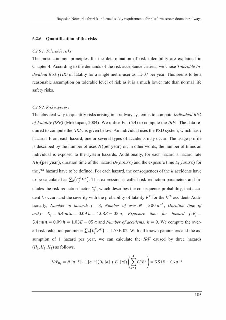
Bayesian Networks for risk-informed safety requirements for platform screen doors in railways
105
6.2.6 Quantification of the risks
6.2.6.1. Tolerable risks
The most common principles for the determination of risk tolerability are explained in
Chapter 4. According to the demands of the risk acceptance criteria, we chose Tolerable In-
dividual Risk (TIR) of fatality for a single metro-user as 1E-07 per year. This seems to be a
reasonable assumption on tolerable level of risk as it is a much lower rate than normal life
safety risks.
6.2.6.2. Risk exposure
The classical way to quantify risks arising in a railway system is to compute Individual Risk
of Fatality (IRF) (Mokkapati, 2004). We utilise Eq. (5.4) to compute the IRF. The data re-
quired to compute the (IRF) is given below. An individual uses the PSD system, which has
hazards. From each hazard, one or several types of accidents may occur. The usage profile
is described by the number of uses or, in other words, the number of times an
individual is exposed to the system hazards. Additionally, for each hazard a hazard rate
, duration time of the hazard and the exposure time for
the hazard have to be defined. For each hazard, the consequences of the accidents have
to be calculated as . This expression is called risk reduction parameters and in-
cludes the risk reduction factor , which describes the consequence probability, that acci-
dent occurs and the severity with the probability of fatality for the accident. Addi-
tionally, Number of hazards: , Number of uses: , Duration time of
ard : , Exposure time for hazard :
and Number of accidents: . We compute the over-
all risk reduction parameter as 1.73E-02. With all known parameters and the as-
sumption of 1 hazard per year, we can calculate the IRF caused by three hazards
( ) as follows.
A Bayesian Network Methodology for Railway Risk, Safety and Decision Support
106
The accumulative individual risk from all three hazards above becomes:
6.2.6.3. Risk assessment
The above calculated risks are now compared with the risk acceptance criteria. It is ob-
served that only the Hazard has tolerable risks (below the TIR (1E-07 per year)). The
other Hazards create higher risks and are not tolerable in accordance to the risk acceptance
criteria. In the end, the overall risks are too high. We need to have a safety technology that
should minimize the accumulative risks above to the acceptable level, say 1E-07 per year.
The is not known for the hazards. According to the individual risks from these hazards,
we can calculate tolerable hazard rates (THR) for each hazard. For this, we take IRF = TIR
as 1E-07 per year and compute the tolerable hazard rate (THR) as:
Bayesian Networks for risk-informed safety requirements for platform screen doors in railways
107
If we apportion the above system level THR to the function level5 we get value lower than
per function. (Here, all safety functions of the PSD technology are not dis-
cussed since the design of technology was in the conceptual phase.) Therefore, the system
level THR calculated above will be within the discrete level that corresponds to SIL 3 (see
Figure 4.3). Therefore, SIL 3 is regarded as the safety requirement for the PSD system. In
other words, the PSD system must demonstrate the lower failures than 1E-07 per hour.
The framework and consequence model offered a suitable solution for one time decision
making problem. The Bayesian Networks based consequence model helped operator, sup-
plier and independent assessor in understanding the influencing factors and their dependen-
cies for the risk assessment of PSD system.
6.3 Summary
The objective of the work was to determine the risk-informed safety requirements for PSD
system located in a megacity. The SIL requirements for the PSD were quantified. The prob-
ability values are based on real operational/infrastructural conditions and data as well as ex-
pert consultations. The models and their assessment in this work are mainly based on proba-
bility, not statistics. The framework and models presented in this chapter are useful because
they have served the purpose; determination of SIL. The reliance of this study on (generic)
model and data associated to the model can be a good approximation to screen the life safe-
ty risks in connection with the PSD system for a URTS in a mega city. The safety technolo-
gy (PSD system) can be declared as TECHNICALLY SUITABLE provided that it fulfils
the SIL 3 requirement for the specific URTS. The conclusions of the risk assessment and the
safety requirements are completely based on the data and general considerations, which
were site, structure and system specific. Models and their values have to be adapted to the
specific environment of other PSD applications in URTS before they can be used for other
risk quantification.
5 SIL is only assigned to the safety functions of a safety technology.
CHAPTER 7: INFLUENCE DIAGRAMS BASED DECISION SUPPORT FOR RAILWAY LEVEL CROSSINGS
7.1 Introduction
In many cases, the problem of risk acceptance turns into an economic decision problem
when the risks are in the so-called tolerable or ALARP region and objective is to further re-
duce the risks. For instance, should we introduce a safety technology if the individual risk
per year is close to the risk acceptance level per year in Figure 7.1? In
this situation, one may require following criteria for decision making on further reduction of
risks:
Tolerate risks if the risk reduction cost is grossly disproportionate to the benefits
achieved; and
Tolerate risks if the risk reduction cost exceeds improvement achieved.
Benefit-Cost-Analysis (BCA) and Willingness-to-Pay (WTP) are commonly applied eco-
nomic based approaches in case the risks are in tolerable region. The BCA and WTP take
into account the same parameters for the comparison of profitability of different safety
measures. Identification of such parameters for different socio-economic and geographical
conditions and assigning monetary values (to benefits and costs) of the identified parameters
has complications. Detail discussion on the BCA and WTP is beyond the scope of this the-
sis. For further readings on the BCA and the WTP and their application to different indus-
tries readers are referred to (Evans, 2013; TD, 2000; Aoun, et al., 2012; RSSB, 2006; Evans,
2005). The WTP and BCA become difficult to apply if the parameters of the decision prob-
lem are not well known. This motivates investigations into an alternative methodology,
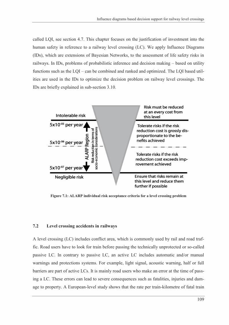
Influence diagrams based decision support for railway level crossings
109
called LQI, see section 4.7. This chapter focuses on the justification of investment into the
human safety in reference to a railway level crossing (LC). We apply Influence Diagrams
(IDs), which are extensions of Bayesian Networks, to the assessment of life safety risks in
railways. In IDs, problems of probabilistic inference and decision making – based on utility
functions such as the LQI – can be combined and ranked and optimized. The LQI based util-
ities are used in the IDs to optimize the decision problem on railway level crossings. The
IDs are briefly explained in sub-section 3.10.
Figure 7.1: ALARP individual risk acceptance criteria for a level crossing problem
7.2 Level crossing accidents in railways
A level crossing (LC) includes conflict area, which is commonly used by rail and road traf-
fic. Road users have to look for train before passing the technically unprotected or so-called
passive LC. In contrary to passive LC, an active LC includes automatic and/or manual
warnings and protections systems. For example, light signal, acoustic warning, half or full
barriers are part of active LCs. It is mainly road users who make an error at the time of pass-
ing a LC. These errors can lead to severe consequences such as fatalities, injuries and dam-
age to property. A European-level study shows that the rate per train-kilometre of fatal train
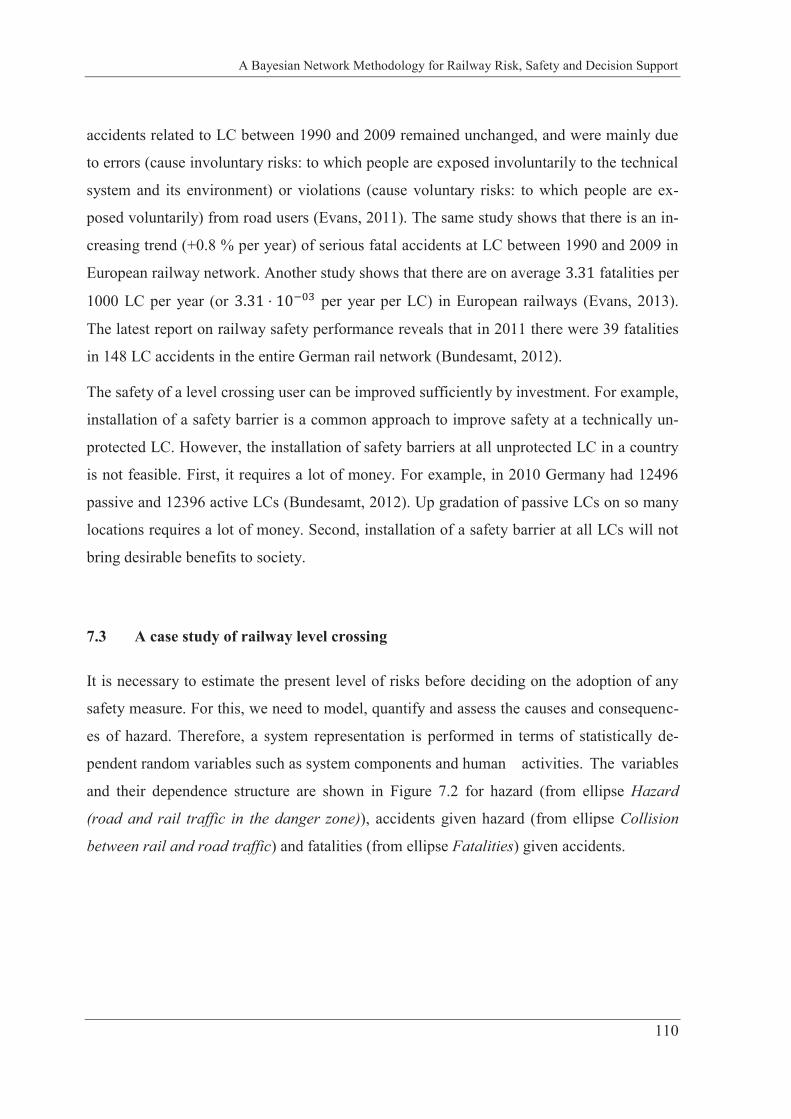
A Bayesian Network Methodology for Railway Risk, Safety and Decision Support
110
accidents related to LC between 1990 and 2009 remained unchanged, and were mainly due
to errors (cause involuntary risks: to which people are exposed involuntarily to the technical
system and its environment) or violations (cause voluntary risks: to which people are ex-
posed voluntarily) from road users (Evans, 2011). The same study shows that there is an in-
creasing trend (+0.8 % per year) of serious fatal accidents at LC between 1990 and 2009 in
European railway network. Another study shows that there are on average fatalities per
1000 LC per year (or per year per LC) in European railways (Evans, 2013).
The latest report on railway safety performance reveals that in 2011 there were 39 fatalities
in 148 LC accidents in the entire German rail network (Bundesamt, 2012).
The safety of a level crossing user can be improved sufficiently by investment. For example,
installation of a safety barrier is a common approach to improve safety at a technically un-
protected LC. However, the installation of safety barriers at all unprotected LC in a country
is not feasible. First, it requires a lot of money. For example, in 2010 Germany had 12496
passive and 12396 active LCs (Bundesamt, 2012). Up gradation of passive LCs on so many
locations requires a lot of money. Second, installation of a safety barrier at all LCs will not
bring desirable benefits to society.
7.3 A case study of railway level crossing
It is necessary to estimate the present level of risks before deciding on the adoption of any
safety measure. For this, we need to model, quantify and assess the causes and consequenc-
es of hazard. Therefore, a system representation is performed in terms of statistically de-
pendent random variables such as system components and human activities. The variables
and their dependence structure are shown in Figure 7.2 for hazard (from ellipse Hazard
(road and rail traffic in the danger zone)), accidents given hazard (from ellipse Collision
between rail and road traffic) and fatalities (from ellipse Fatalities) given accidents.
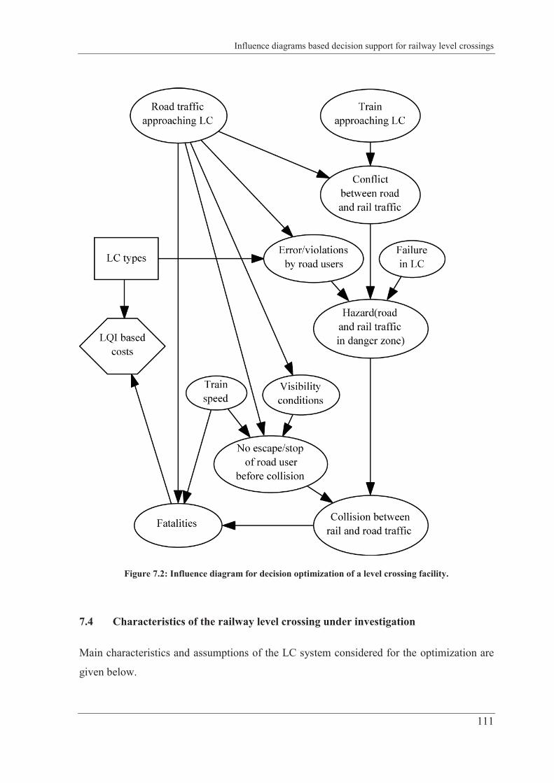
Influence diagrams based decision support for railway level crossings
111
Figure 7.2: Influence diagram for decision optimization of a level crossing facility.
7.4 Characteristics of the railway level crossing under investigation
Main characteristics and assumptions of the LC system considered for the optimization are
given below.

A Bayesian Network Methodology for Railway Risk, Safety and Decision Support
112
The LC is located on a single track.
There is one train demand at a time.
We consider two main causes of collisions; Human errors/violations by road users
and technical failures in LC. The technical failures in active level crossings are rare
and considered constant ( per hour) for all types of LCs.
Train driver is not making errors/violations at LC.
All active LCs are automatic. In other words, the operation of the active LC does not
require the aid of a gateman.
Conflict area of LC with full barrier is supervised by the additional detection tech-
nology, which further control hazards. The train will stop in case the conflict area is
occupied by the road users.
We assume that installation of half barrier and light signal technologies always allow
road users to escape from the conflict area.
We do not consider risks resulting from traffic queues after passing the LC.
We only consider head-on collisions. It means that road traffic has very low possibil-
ity of hitting a train side. For this reason, we consider train head as an impact point.
This point needs maximum 1 sec to pass the conflict area.
Three different levels of speeds (low<60, 60<moderate<120, 120<high) are consid-
ered. The higher speed will lead to higher consequences, given the hazard as well as
accidents.
Probability values are calculated on the basis of yearly data.
We do not consider the time dependent behaviour of a road user. In other words,
road users have different error probabilities towards closing time of different level
crossing barriers.
The objective of the study here is to show the application of the IDs and LQI to railway risk
optimization, and not to show the detailed risk analysis of a LC. Therefore, we do not dis-
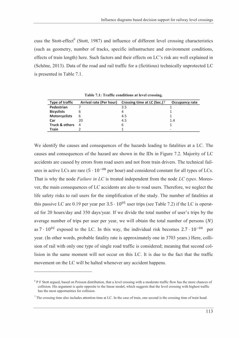
Influence diagrams based decision support for railway level crossings
113
cuss the Stott-effect6 (Stott, 1987) and influence of different level crossing characteristics
(such as geometry, number of tracks, specific infrastructure and environment conditions,
effects of train length) here. Such factors and their effects on LC’s risk are well explained in
(Schöne, 2013). Data of the road and rail traffic for a (fictitious) technically unprotected LC
is presented in Table 7.1.
Table 7.1: Traffic conditions at level crossing.
Type of traffic Arrival rate (Per hour) Crossing time at LC (Sec.) Occupancy rate Pedestrian 7 3.5 1 Bicyclists 6 4 1 Motorcyclists 6 4.5 1 Car 20 4.5 1.4 Truck & others 4 6 1 Train 2 1 -
We identify the causes and consequences of the hazards leading to fatalities at a LC. The
causes and consequences of the hazard are shown in the IDs in Figure 7.2. Majority of LC
accidents are caused by errors from road users and not from train drivers. The technical fail-
ures in active LCs are rare ( per hour) and considered constant for all types of LCs.
That is why the node Failure in LC is treated independent from the node LC types. Moreo-
ver, the main consequences of LC accidents are also to road users. Therefore, we neglect the
life safety risks to rail users for the simplification of the study. The number of fatalities at
this passive LC are 0.19 per year per user trips (see Table 7.2) if the LC is operat-
ed for 20 hours/day and 350 days/year. If we divide the total number of user’s trips by the
average number of trips per user per year, we will obtain the total number of persons
as exposed to the LC. In this way, the individual risk becomes per
year. (In other words, probable fatality rate is approximately one in 3703 years.) Here, colli-
sion of rail with only one type of single road traffic is considered; meaning that second col-
lision in the same moment will not occur on this LC. It is due to the fact that the traffic
movement on the LC will be halted whenever any accident happens.
6 P F Stott argued, based on Poisson distribution, that a level crossing with a moderate traffic flow has the more chances of collision. His argument is quite opposite to the linear model, which suggests that the level crossing with highest traffic has the most opportunities for collision.
7 The crossing time also includes attention time at LC. In the case of train, one second is the crossing time of train head.
A Bayesian Network Methodology for Railway Risk, Safety and Decision Support
114
Table 7.2: Individual risks from different types of level crossings.
LC types collisions (Per year) Fatalities (Per year) Individual risk of fatality (Per year)
Passive LC 0.74 0.19 Light signal 0.10 0.03 Half barrier 0.0138 0.0054 Full barrier 0.0035 0.002
Now, based on the ALARP criteria in Figure 7.1, the individual risk value per
year is not lying within the tolerable region. Therefore, target becomes to reduce the IRF at
this LC. Depending on operation, socio-economic and environmental conditions of traffic
system, different types of safety measures can be adopted for the LC. In this study, we in-
vestigate the effects of following three safety measures on life safety risks:
Light signal: it is fitted with optical and acoustic warnings,
Half barrier: it is fitted with optical warnings and protects the road users with half barrier,
Full barrier: it is fitted with optical warnings and protects the road users with full barrier. In
Germany, this type of level crossing protection also supervises conflict area8. It means that
the train is not allowed to pass the LC if the conflict area is occupied by the road traffic.
There will be decrease in individual risk if one of the above safety measures is adopted for
the LC. We investigate expected collisions, fatalities and individual risks for different types
of LCs. Here, assumption is made that all the operation and environment conditions remain
the same at the LC. In Table 7.2, the decrease in fatality rate is mainly influenced by human
error probabilities (HEP). The road users have different error and visibility probabilities to-
wards particular safety barrier. For example, HEP and visibility would be higher for a pe-
destrian than a car user at the same LC. For pedestrians and cyclists one should consider
high risk values because they are always able to override the technical protections. These
factors are considered in Figure 7.2 for all LCs.
Table 7.2 shows that one can achieve high safety level if the technically unprotected LC is
replaced with one of the active LCs above. Installation of the active LCs can bring the IRF
to the ALARP region in Figure 7.1. It is to mention that the long term objective of risk man-
8 An area that can jointly be occupied by road and rail traffic is called conflict area,
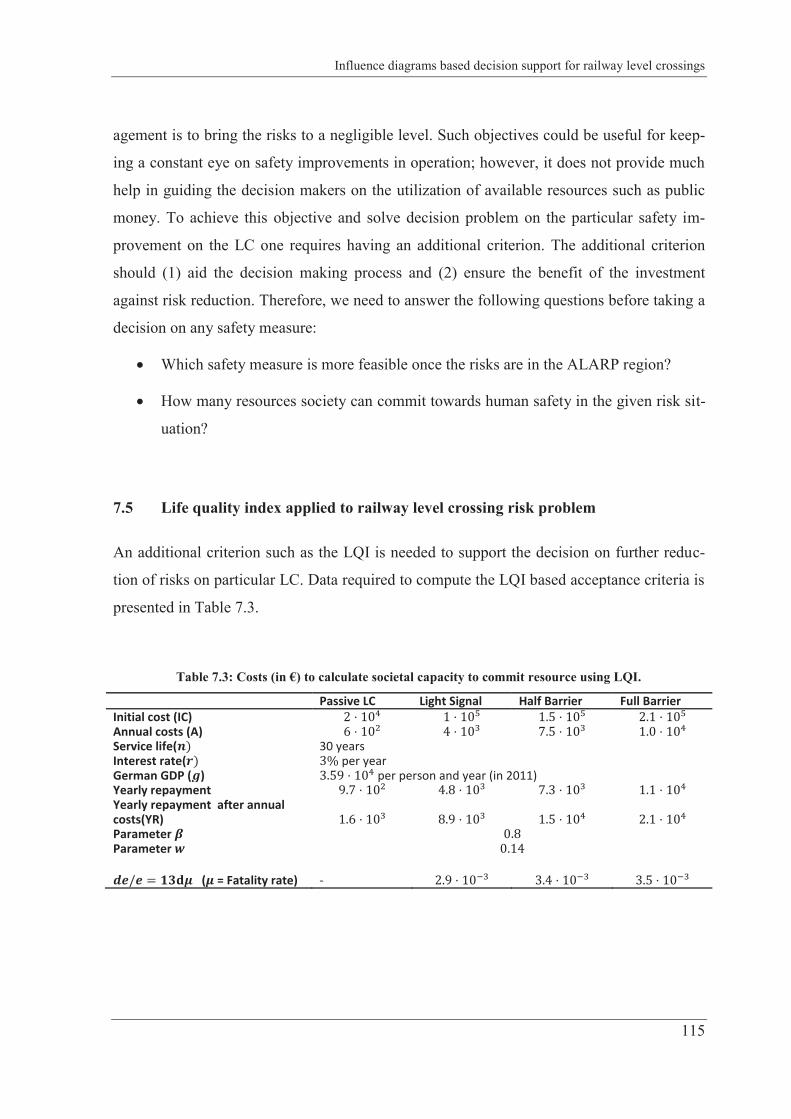
Influence diagrams based decision support for railway level crossings
115
agement is to bring the risks to a negligible level. Such objectives could be useful for keep-
ing a constant eye on safety improvements in operation; however, it does not provide much
help in guiding the decision makers on the utilization of available resources such as public
money. To achieve this objective and solve decision problem on the particular safety im-
provement on the LC one requires having an additional criterion. The additional criterion
should (1) aid the decision making process and (2) ensure the benefit of the investment
against risk reduction. Therefore, we need to answer the following questions before taking a
decision on any safety measure:
Which safety measure is more feasible once the risks are in the ALARP region?
How many resources society can commit towards human safety in the given risk sit-
uation?
7.5 Life quality index applied to railway level crossing risk problem
An additional criterion such as the LQI is needed to support the decision on further reduc-
tion of risks on particular LC. Data required to compute the LQI based acceptance criteria is
presented in Table 7.3.
Table 7.3: Costs (in €) to calculate societal capacity to commit resource using LQI.
Passive LC Light Signal Half Barrier Full Barrier Initial cost (IC) Annual costs (A) Service life( 30 years Interest rate( per year German GDP ( ) per person and year (in 2011) Yearly repayment Yearly repayment after annual costs(YR) Parameter Parameter
( = Fatality rate) -
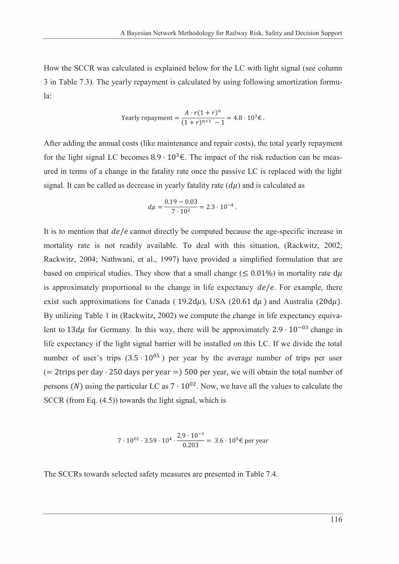
A Bayesian Network Methodology for Railway Risk, Safety and Decision Support
116
How the SCCR was calculated is explained below for the LC with light signal (see column
3 in Table 7.3). The yearly repayment is calculated by using following amortization formu-
la:
After adding the annual costs (like maintenance and repair costs), the total yearly repayment
for the light signal LC becomes . The impact of the risk reduction can be meas-
ured in terms of a change in the fatality rate once the passive LC is replaced with the light
signal. It can be called as decrease in yearly fatality rate ( ) and is calculated as
It is to mention that cannot directly be computed because the age-specific increase in
mortality rate is not readily available. To deal with this situation, (Rackwitz, 2002;
Rackwitz, 2004; Nathwani, et al., 1997) have provided a simplified formulation that are
based on empirical studies. They show that a small change ( ) in mortality rate
is approximately proportional to the change in life expectancy . For example, there
exist such approximations for Canada ( ), USA ( and Australia ( .
By utilizing Table 1 in (Rackwitz, 2002) we compute the change in life expectancy equiva-
lent to for Germany. In this way, there will be approximately change in
life expectancy if the light signal barrier will be installed on this LC. If we divide the total
number of user’s trips ( ) per year by the average number of trips per user
( per year, we will obtain the total number of
persons using the particular LC as . Now, we have all the values to calculate the
SCCR (from Eq. (4.5)) towards the light signal, which is
The SCCRs towards selected safety measures are presented in Table 7.4.
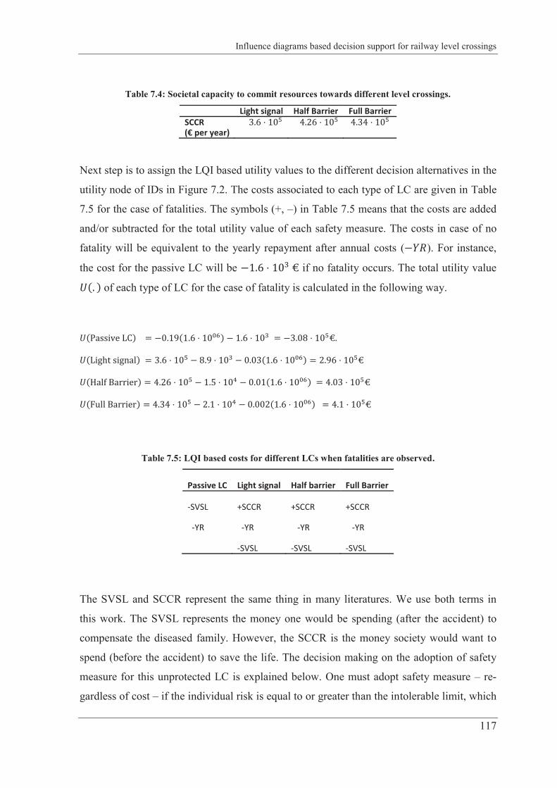
Influence diagrams based decision support for railway level crossings
117
Table 7.4: Societal capacity to commit resources towards different level crossings.
Light signal Half Barrier Full Barrier SCCR (€ per year)
Next step is to assign the LQI based utility values to the different decision alternatives in the
utility node of IDs in Figure 7.2. The costs associated to each type of LC are given in Table
7.5 for the case of fatalities. The symbols (+, –) in Table 7.5 means that the costs are added
and/or subtracted for the total utility value of each safety measure. The costs in case of no
fatality will be equivalent to the yearly repayment after annual costs ( ). For instance,
the cost for the passive LC will be if no fatality occurs. The total utility value
of each type of LC for the case of fatality is calculated in the following way.
Table 7.5: LQI based costs for different LCs when fatalities are observed.
Passive LC
Light signal
Half barrier
Full Barrier
-SVSL
+SCCR
+SCCR
+SCCR
-YR
-YR
-YR
-YR
-SVSL
-SVSL
-SVSL
The SVSL and SCCR represent the same thing in many literatures. We use both terms in
this work. The SVSL represents the money one would be spending (after the accident) to
compensate the diseased family. However, the SCCR is the money society would want to
spend (before the accident) to save the life. The decision making on the adoption of safety
measure for this unprotected LC is explained below. One must adopt safety measure – re-
gardless of cost – if the individual risk is equal to or greater than the intolerable limit, which
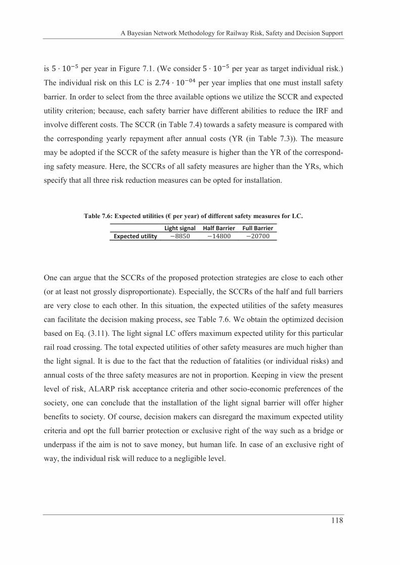
A Bayesian Network Methodology for Railway Risk, Safety and Decision Support
118
is per year in Figure 7.1. (We consider per year as target individual risk.)
The individual risk on this LC is per year implies that one must install safety
barrier. In order to select from the three available options we utilize the SCCR and expected
utility criterion; because, each safety barrier have different abilities to reduce the IRF and
involve different costs. The SCCR (in Table 7.4) towards a safety measure is compared with
the corresponding yearly repayment after annual costs (YR (in Table 7.3)). The measure
may be adopted if the SCCR of the safety measure is higher than the YR of the correspond-
ing safety measure. Here, the SCCRs of all safety measures are higher than the YRs, which
specify that all three risk reduction measures can be opted for installation.
Table 7.6: Expected utilities (€ per year) of different safety measures for LC.
Light signal Half Barrier Full Barrier Expected utility
One can argue that the SCCRs of the proposed protection strategies are close to each other
(or at least not grossly disproportionate). Especially, the SCCRs of the half and full barriers
are very close to each other. In this situation, the expected utilities of the safety measures
can facilitate the decision making process, see Table 7.6. We obtain the optimized decision
based on Eq. (3.11). The light signal LC offers maximum expected utility for this particular
rail road crossing. The total expected utilities of other safety measures are much higher than
the light signal. It is due to the fact that the reduction of fatalities (or individual risks) and
annual costs of the three safety measures are not in proportion. Keeping in view the present
level of risk, ALARP risk acceptance criteria and other socio-economic preferences of the
society, one can conclude that the installation of the light signal barrier will offer higher
benefits to society. Of course, decision makers can disregard the maximum expected utility
criteria and opt the full barrier protection or exclusive right of the way such as a bridge or
underpass if the aim is not to save money, but human life. In case of an exclusive right of
way, the individual risk will reduce to a negligible level.
Influence diagrams based decision support for railway level crossings
119
7.6 Summary
Life safety risks from a technically unprotected railway LC were modelled, quantified and
optimized using the IDs. The risks were assessed using the ALARP criteria, which is useful
in differentiating the tolerable and intolerable risks in railways. It was required to reduce the
risk on the LC; because, the IRF on the LC were in the intolerable region. The societal ca-
pacity to commit resources (SCCR) based on the LQI criterion was utilized in selecting a
suitable safety barrier. Expected utilities of different decision alternatives were computed
using a prior decision analysis. The light signal safety barrier offered maximum expected
utility for a particular LC. Thus, the optimal decision is to replace the unprotected LC, at
least, with the light signal LC. We conclude that the LQI provided an additional decision
support towards the adaptation of risk mitigating measures for a railway facility when the
risks were in the ALARP region. In other words, it offered a rational mean to implement the
ALARP. The IDs, which utilized the LQI based utilities, offered an improved framework
for quantitative risk assessment, acceptability and optimality of the railway risks.
CHAPTER 8: CONCLUSIONS AND OUTLOOK
8.1 Summary and important contributions
Railway systems are rather complex and require the investigation of new methods, models,
tools and techniques for modelling and analysis of their risks. This thesis mainly focuses on
the application of Bayesian Networks to complex railway systems. We propose a Bayesian
Networks methodology for railway risk, safety and decision support. Bayesian Networks are
applied to one example application and two real-world problems. It is shown that Bayesian
Networks have a number of useful characteristics that are suitable for many risk and safety
problems in railways, especially those that involve dependencies, uncertainties and addi-
tional knowledge. Bayesian Networks are able to model and update information in complex
railways and the problem of probabilistic inference and decision making can be combined
and optimized. As a result, risk-based decision alternatives in railways can be ranked.
The first contribution of the thesis certainly consists of addressing some specific issues that
arise in the modelling and analysis of risk-based safety in complex railways. A problem of
complex railways – characterized by the presence of dependencies and uncertainties in the
system – is presented in Chapter 5. These dependencies and uncertainties arose due to
common causes, disjoint events, failure dependency, functional uncertainty, multistate
events and additional considerations on expert knowledge in the risk models. Failing to con-
sider such complex aspects leads to over estimation of the system risks. FTA, being a classi-
cal method, had limitations in dealing with the example application from complex railways.
However, Bayesian Networks were able to handle large numbers of top events, intermediate
events, uncertainties and dependencies in complex railways in concise and flexible way. No
repetition of the random variables (events in the risk model) was required to introduce such
dependencies and uncertainties.
Conclusions and outlook
121
The second contribution of this thesis consists of the computation of a number of IMs for
complex systems using Bayesian Networks. It was shown that the computation of a number
of IMs for a complex railway system is straightforward using standard Bayesian inference.
By exploiting the use of updating properties of the Bayesian Networks, failing as well as
working components of the railway system can be identified and ranked at the same time
using appropriate importance measures.
The third contribution of this thesis consists of the application of Bayesian Networks to a
real-world railway problem. A Bayesian Networks based consequence model was developed
to quantify the risk reduction factor for a PSD system, installed for a URTS in a mega city.
Safety integrity requirements (the so-called SILs) of the safety technology were determined
using the consequence model. The Bayesian Networks based graphical representation of the
consequence model helped in better understanding the risk’s influencing factors and inter-
and-intra dependencies among them, especially to the stakeholders (such as suppliers, op-
erators and other system experts) who were not experts in probabilistic risk assessment.
Bayesian Networks offered a suitable technique to (1) model relevant information and (2)
quantify risk factors for a safety technology in railways. This consequence model was ac-
cepted by the concerned railway authorities.
The fourth contribution of this thesis consists of the joint treatment of ALARP and a utility
based acceptability criterion and the consequence models for railways. In addition to the
widely applied ALARP, MEM and MGS criteria, we applied the LQI risk acceptance crite-
ria. IDs, which are extensions of Bayesian Networks, were utilized in the assessment of life
safety risks in a railway LC problem. LQI-based utilities were used (1) to quantify the
SCCR towards saving a life on the railways and (2) in the IDs to optimize the decision prob-
lems on a (fictitious) railway LC. We showed that utility based risk acceptance criteria, such
as the LQI, give a useful decision aid in justifying the investment in human safety, especial-
ly in the case of a railway LC. Further, the LQI provided a means to implement the ALARP
criteria.
The use of Bayesian Networks in railway risk and safety is rare. This study shows the suita-
bility of a Bayesian Network based framework towards risk-based decision aid in railways.
The suitability is shown through an example application and real world applications. Bayes-
A Bayesian Networks Methodology for Railway Risk, Safety and Decision Support
122
ian Networks provided a useful tool for modelling, assessing and optimizing risks on rail-
ways.
8.2 Originality of the work
With respect to the originality of the work, it is stated that the main contributions of the the-
sis are concentrated in Chapters 5, 6 and 7. Most of the work presented in these chapters has
not been conducted by any other researcher so far. This includes (1) the mapping of ad-
vanced aspects of fault trees into Bayesian Networks for railways and (2) the computation
of the IMs for complex railways using Bayesian Networks (Chapter 5). A framework for
determining the safety integrity requirements for PSD in railways is presented. A Bayesian
Networks based consequence model was developed for a particular railway application
(Chapter 6). An IDs based decision optimization framework was introduced for a railway
LC problem. Application of the LQI, in combination with the ALARP approach, to railway
risk acceptance is presented (Chapter 7).
8.3 Outlook
Throughout the present thesis, the research focus is mainly on the application of Bayesian
Networks. The presented thesis addresses some parts of the issues that arise in the modelling
and analysis of risk-based safety in complex railways and how they can be handled using
Bayesian Networks. It should be noted that the models and their probability values in the
thesis are based on particular operational/infrastructural conditions and data as well as ex-
pert consultations. Therefore, the conclusions of the risk assessment and the safety require-
ments are completely based on the data and general considerations, which are site, structure
and system specific. Thus, models and their values have to be adapted to the specific opera-
tional environments of other similar railway applications, before they can be used for risk
quantification and decision support. It implies that further studies are needed before these
models and methods are applied elsewhere.

Conclusions and outlook
123
The scope of the thesis does not include the development of a universal risk management
tool – a deliverable mature product – for railway operators. However, this thesis provides a
foundation that can be used to develop an ID-based applied tool for railway risk manage-
ment. Significant progress is possible if the developments in decision formulations for addi-
tional applications in the field of railways are made. For instance, an ID-based decision sup-
port tool for an individual railway facility, railway line or complete network can be intro-
duced. This decision support system may include a number of hazards, a variety of influenc-
ing variables for hazards and, inter – and – intra dependencies among the hazards and uncer-
tainties. Different decision alternatives and mitigating measures, together with their utilities,
can be incorporated into the IDs. In most cases, time dependencies have great influence on
the quantified risk assessment. For instance, road traffic such as pedestrians and cyclists
have higher violations probabilities and possibilities, after the safety barrier has been closed
at a railway LC. The errors are not time dependent; however, the violations are a function of
the closing time of the barriers (and the type of barrier). In other words, the longer is the
closing time of the barrier the higher the probability of violation. In this way, the change in
the expected fatalities in the next time step, say after three minutes of waiting at an LC, can
have an influence on risk-based decision making because the probability of an accident can
increase with the passage of time due to the increased tendency of the road users to violate
the safety barrier. It implies that the expected fatalities at the barriers are a function of time.
The modelling of such a dynamic violation behaviour of the user is possible using dynamic
Bayesian Networks. Additionally, the proposed decision support methodology can be ex-
tended beyond railway accidents or safety cases. It can be expanded to consider other haz-
ards, such as earthquakes, fires and floods, that can have sever effects on the safety and reli-
ability of a railway transport system. The Bayesian Networks based methodology presented
in this study offers such expansion. However, the decision models should be constructed in
close collaboration with actual experts and decision-makers such as transport authorities,
operators and insurance companies.
BIBLIOGRAPHY
Ahmed, R., 2010. Bayesian Network. Rijeka: Sciyo. Anders, E., 2008. Ein Beitrag zur komplexen Sicherheitsbetrachtung des Bahnsystems, TU
Dresden: PhD dissertation. Andrews, J. D. & Moss, T. R., 1993. Reliability and risk assessment. s.l.:John Wiley and
Sons. Aoun, R. B., Koursi, E.-M. & Lemaire, E., 2012. The cost benefit analysis of level crossing
safety measures. In: Computers in Railways Xll. Southampton: WIT press, pp. 851-862.
Aven, T., 2008. Risk analysis. West Sussex: John Wiley & Sons. Aven, T., 2011. QUANTITATIVE RISK ASSESSMENT: The Scientific Platform. New York:
Cambridge University Press. Aven, T., 2012. Foundational Issues in Risk Assessment and Risk Management. Risk
Analysis, 32(10), pp. 1647-1655. Bearfield, G. & Marsh, D. W. R., 2005. Generalising Event Trees using Bayesian Networks
with a Case Study of Train Derailment. s.l., LNCS 3688, pp. 52-66. Benjamin, J. & Cornell, C., 1970. Probability, Statistics, and Decisions for Civil Engineers.
New York: McGraw-Hill. Bensi, M., 2010. A Bayesian Network Methodology for Infrastructure Seismic Risk
Assessment and Decision Support, UC Berkeley: PhD thesis. Bensi, M., Der Kiureghian, A. & Straub, D., 2011. A Bayesian Network Methodology for
Infrastructure Seismic Risk Assessment and Decision Support, College of Engineering, University of California, Berkeley: PEER Report 2011/02, Pacific Earthquake Engineering Research Center.
Bernardo, J. M. & Smith, A. F. M., 2000. Bayesian Theory. West Sussex: JOHN WILEY & SONS, LTD.
Beugin, J., Renaux, D. & Cauffriez, L., 2007. A SIL quantification approach based on an operating situation model for safety evaluation in complex guided transportation systems. Reliability Engineering & System Safety, Volume 92, pp. 1686-1700.
Birnbaum, Z. W., 1969. On the importance of different components in a multi-component system. In Multivariable Analysis II, P.R. Kor-ishnaiah, Ed, New York,NY: Academic Press.
Bobbio, A., Portinale, L., Minichino, M. & Ciancamerla, E., 2001. Improving the analysis of dependable systems by mapping fault trees into Bayesian networks. Reliability Engineering and Systen Safety 71, pp. 249-260.
Borgonovo, E. & Apostolakis, G., 2001. A new importance measure for risk-informed decision making. Reliability Engineering & System Safety, 72(2), pp. 193-212.
Borgonovo, E., Apostolakis, G. E., Tarantola, S. & Saltelli, A., 2003. Comparison of global sensitivity analysis techniques and importance measures in PSA. Reliability Engineering & System Safety,79(2), pp. 175-185.
Borgonovo, E. & Smith, C., 2011. A study of Interactions in the Risk Assessment of Complex Engineering Systems: An Application to Space PSA. Operations Research, 59(6), pp. 1461-1476.
Bowles, J. B., 2002. Commentary-Caution: Constant Failure-Rate Models May be Hazardous to Your Design. IEEE TRANSACTIONS ON RELIABILITY , 51(3), pp. 375-377.
125
Braband, J., 2001. A Practical Guide to Safety Analysis Methods. SIGNAL+DRAHT, 93(9), pp. 41-44.
Braband, J., 2010. On the Justification of a Risk Matrix for Technical Systems in European Railways . In: E. Schneider & G. Tarnai, eds. FORMS/FORMAT . Heidelberg: Springer, pp. 185-192.
Braband, J. et al., 2006. The CENELEC-Standards regarding Functional Safety, Hamburg: Eurailpress.
Braband, J. & Lennartz, K., 2000. Risk-oriented apportionment of safety integrity requirements-an example. SIGNAL+DRAHT, pp. 35-39.
Bucher, C., 2009. Computational Analysis of Randomness in Structural Mechanics. Structures and Infrastructures Book Series, Vol. 3 ed. Leiden: CRC Press.
Bundesamt, S., 2012. Betriebsdaten des Schienenverkehrs 2011, Wiesbaden: Statistisches Bundesamt.
CENELEC, 2012. European Committee For Electronic Standardization. [Online] Available at: http://www.cenelec.eu/index.html [Accessed 06 2013].
Chen, S., Ho, T. & Mao, B., 2007. Reliability evaluations of railway power supplies by fault-tree analysis. doi: 10.1049/iet-epa:20060244, s.n., pp. 161-172.
Cheok, M. C., Parry, G. W. & Sherry, R. R., 1998. Use of importance measures in risk-informed regulatory applications. Reliability Engineering and System Safety , Volume 60, pp. 213-226.
Darwiche, A., 2010. What are Bayesian networks and why are their applications growing across all fields?. Communications of the ACM, 53(12), pp. 80-90.
Der Kiureghian, A., 2005. First- and second-order reliability methods. In: E. N. e. al., ed. Chapter 14, in Engineering design reliability handbook. Boca Raton: CRC.
Dhillon, B., 2007. Human Reliability and Error in Transportation Systems. London: Springer.
Dhillon, B., 2011. Transportaiton Systems Reliability and Safety. 1st ed. Boca Raton: CRC. ERA, 2013. Intermediate report on the development of railway safety in the European
Union. [Online] Available at: http://www.era.europa.eu/Core-Activities/Safety/Safety-Performance/Pages/Safety-Performance-Report.aspx [Accessed 07 06 2013].
Ericson, C. A., 2005. Hazard Analysis Techniques for System Safety. New Jersey: John Wiley & Sons.
EU, 2012. EU TRANSPORT IN FIGURES: STATISTICAL POCKETBOOK, Luxembourg: European Union.
Evans, A., 2011. Fatal Train Accidents On Europe`s Railways: 1980-2009. Accident Analysis and Prevention, 43(1(391-401)).
Evans, A. W., 2003. Estimating transport fatality risk from past accident data. London: Elsevier.
Evans, A. W., 2005. Railway Risks, Safety Values and Safety Costs. Transport, part of the Proceedings of the Institution of Civil Engineers, 158(TRI), pp. 3-9.
Evans, A. W., 2013. THE ECONOMICS OF RAILWAY SAFETY. Research in Transport Economics, p. 10.1016/j.retrec.2012.12.003.
Faber, M. H., 2012. Statistics and Probability Theory: In Pursuit of Engineering Decision Support. Topics in Safety, Risk, Reliability and Quality, Vol. 18 ed. s.l.:Springer.
126
Faber, M. H., Straub, D., Montes-Iturrizaga, R. & Heredia-Zavoni, E., 2012. Risk Assessment for Design of FPSO Systems. Part I: Generic Models and Acceptance Criteria. Marine Structures, 28(1), pp. 120-133.
Flammini, F., Gglione, A., mazzocca, N. & Pragliola, C., 2009. Quantitative Security Risk Assessment and Management for Railway Transportation Infrastructures. In: R. S. a. S. G. (Eds.), ed. CRITIS 2008. Berlin Heidelberg: Springer-Verlag, pp. 180-189.
Ford, R., 2001. Modern Railways. The Forgotten Driver, January, pp. 45-48. Fussell, B., 1975. How to hand-calculate system reliability characteristics. IEEE Trans. on
Reliability, p. 24(3). Gelman, A., Carlin, J. B., Stern, H. S. & Rubin, D. B., 2009. Bayesian Data Analysis. 2nd
ed. Florida: CRC . Hanea, D. & Ale, B., 2009(b). Risk of human fatalities in building fires: A decision tool
using Bayesian Networks. Fire Safety, Volume 44(5), pp. 704-710. Hanea, D. M., 2009(a). Human Risk of Fire: Building a decision support tool using
Bayesian Networks, TU Delft: PhD thesis. Heredia-Zavoni, E., Montes-Iturrizaga, R., Faber, M. & Straub, D., 2012. Risk assessment
for structural design criteria of FPSO systems. Part II: Consequence models and applications to determination of target reliabilities. Marine Structures, Volume 28, pp. 50-66.
Holicky, M. & Diamantidis, D., 2008. Optimization of Road Tunnel Safety. Beton- und Stahlbetonbau, Special Edition, Issue 103.
Holmgren, M., 2005. Maintenance-related losses at the Swedish rail. Quality in Maintenance Engineering, 11(1), pp. 5-18.
IEC 61508, 2000. Functional safety of electrical/electronic/programmable electronic safety-related systems(IEC 61508-1 to 7), Geneva: IEC(International Electronical Commission).
IRSC, I. R. S. C., 2008. Rail Optimization and Safety Analysis. [Online] Available at: http://www.intlrailsafety.com/DenverConference2008.html [Accessed 15 January 2010].
Jensen, F. V. & Nielsen, T. D., 2007. Bayesian Networks and Decision Graphs. Berlin: Springer.
Kalos, M. H. & Whitlock, P., 2004. Monte Carlo Methods. 1st ed. VCH-Verlag: Wiley. Kang, D., Kim, K. & Ha, J., 2002. Importance Analysis of In-Service Testing Components
for Ulchin Unit 3 Using Risk-Informed In-Service Testing Approach. Journal of the Korean Nuclear Society, 33(4), pp. 331-343.
Kerbs, H., Trung, B. L., Koursi, E. M. E. & Firpo, P., 2000. Minimale Endogene Mortalität-ein universelles Sicherheitskriterium. ETR - Eisenbahntechnische Rundschau, 49(12), pp. 816-821.
Khakzad, N., Khan, F. & Amyotte, P., 2011. Safety Analysis in Process Facilities: Comparison of Fault Tree and Bayesian Network Approaches. Reliability Engineering and System Safety, p. doi:10.1016/j.ress.2011.03.012.
Khakzad, N., Khan, F. & Amyotte, P., 2013. Dynamic safety analysis of process systems by mapping bow-tie into Bayesian network. Process Safety and Environmental Protection, 91(1-2), pp. 46-53.
Kiureghian, A. D., 2005. First- and Second-Order Reliability Methods. In: E. Nikilaidis, D. M. Ghiocel & S. Singhal, eds. Engineering Design Reliability Handbook. s.l.:CRC Press, p. Chapter 14.
127
Kjaerulff, U. B. & Madsen, A. L., 2007. Bayesian Networks and Influence Diagrams: A Guide to Construction and Analysis. New York: Springer.
Koller, D. & Friedman, N., 2009. Probabilistic Graphical Models-Principles and Techniques. ISBN-10: 0-262-01319-3: MIT Press.
Kottegoda, N. T. & Rosso, R., 2008. APPLIED STATISTICS FOR CIVIL AND ENVIRONMENTAL ENGINEERS. West Sussex: Blackwell Publishing Ltd.
Lampis, M. & Andrews, J. D., 2009. Bayesian Belief Networks for System Fault Diagnostics. Quality and Reliability Engineering International, pp. 409-426.
Lentz, P., 2007. Acceptablity of civil engineering decisions involving human consequences, PhD thesis, s.l.: lehrstuhl für Massivbau, Technische Universität München.
Lindley, D., 1982a. The Bayesian approach to statistics:In Some Recent Advances in Statistics. London: Academic Press.
Lu, Y., Li, Q. & Hinze, J., 2011. Subway System Safety Risk Analysis Based on Bayesian Network. Computational Risk Management, DOI: 10.1007/978-3-642-15243-6_25(Part 5), pp. 219-227.
Mahboob, Q., Kunze, M., Radczimanowski, G. & Trinckauf, J., 2013. RISK-INFORMED SAFETY REQUIREMENT OF PLATFORM SCREEN DOORS FOR URBAN RAIL TRANSIT SYSTEM IN A MEGA CITY. Amsterdam, ESREL 2013 conference proceedings.
Mahboob, Q., Kunze, M., Trinckauf, J. & Maschek, U., 2012(a). A Flexible and Concise Framework for Hazard Quantification: An Example from Railway Signalling System. Proceedings of the QR2MSE, Chengdu, IEEE Xplore.
Mahboob, Q., Schoene, E., Kunze, E. & Trinckauf, J., 2012(b). Application of importance measures to transport industry: Computation using Bayesian networks and Fault Tree Analysis. Chengdu, IEEE Xplore.
Mahboob, Q. et al., 2012(c). REPRESENTING ADVANCED ASPECTS OF FAULT TREES INTO BAYESIAN NETWORKS - MODELLING SAFETY IN COMPLEX RAILWAY SYSTEMS. In: 9781622764365, ed. 11th International Probabilistic Safety Assessment and Management Conference and the Annual European Safety and Reliability Conference. Helsinki, Finland: Curran Associates, Inc., pp. 711-718.
Mahboob, Q. et al., 2012(d). COMPUTATION OF COMPONENT IMPORTANCE MEASURES FOR RELIABILITY OF COMPLEX SYSTEMS. In: E. E. K. F. T. B. Cengiz Kahraman, ed. Uncertainty modeling in knowledge engineering and decision making. edited by Kahraman, C. et al. ed. FLINS 2012 proceedings, Istanbul: World Scientific Publishing, pp. 1051-1057.
Marsh, W. & Bearfield, G., 2007. Representing Parametrized Fault Trees Using Bayesian Networks. Heidelberg, Springer, pp. 120-1333.
Maschek, U., 2012. SICHERUNG DES SCHIENENVERKEHRS: GRUNDLAGEN UND PLANUNG DER LEIT- UND SICHERUNGSTECHNIK. ISBN: 978-3-8348-1020-5 ed. Wiesbaden: Springer Vieweg.
Melchers, R., 2001. On the ALARP approach to risk management. Reliability Engineering and System Safety, 71(2), pp. 201-208.
Misra, K. B., 2008. THE HANDBOOK OF PERFORMABILITY ENGINEERING. London: Springer-verlag.
Modarres, M., 2008. Probabilistic Risk Assessment. In: K. B. (. Misra, ed. Handbook of Performability Engineering. s.l.:Springer, pp. 699-718.
128
Mohaghegh, Z., Kazemi, R. & Mosleh, A., 2009. Incorporating Organizational Factors into Probabilistic Risk Assessment (PRA) of Complex Socio-technical Systems: A Hybrid Technique Formalization. Reliability Engineering & System Safety, 94(5), pp. 1000-1018.
Mokkapati, C., 2004. A practical risk and safety assesment methodology for safety-critical systems. Nashville, Proceedings of the AREMA 2004 Annual Conferences.
Murphy, K. P., 2002. Dynamic Bayesian Networks: Representation, Inference and Learning, UC Berkely: PhD thesis.
NASA, 2002. Fault Tree Handbook with Aerospace Applications. Washington, DC: NASA Office of Safety and Mission Assurance.
Nathwani, J. S., Lind, N. & Pandey, M., 1997. Affordable safety by choice: the life quality method. Waterloo, Canada: Institute for Risk Research, University of Waterloo.
Nelson, D. & O'Neil, K., 2000. Commuter rail-service reliability: On time performance and causes of delays. Transportation Research Board, Issue 1704, pp. 42-50.
Nishijima, K., 2012. Lecture notes (Summer semester 2012): Engineering Risk and Decision Analysis, Lyngby: CERDA: Technical University of Denmark.
Oukhellou, L., Côme, E., Bouillaut, L. & Aknin, P., 2008. Combined use of sensor data and structural knowledge processed by Bayesian network: Application to a railway diagnosis aid scheme. Transportation Research Part C: Emerging Technologies,Volume 16, Issue 6, pp. 755-767 .
Podofillini, L., Zio, E. & Vatn, J., 2006. Risk-informed optimisation of railway tracks inspection and maintenance procedures.. Reliability Engineering and System Safety, 91(1), pp. 20-35.
Prescott, D. & Andrews, J., 2010. Component Importance Measures To Identify Contributions To System Failure For Aircraft Which Dispatch With Known Faults. Taylor Francis. 675-682, ESREL 2010.
Puettner, R. & Geisler, M., 2008. ROSA - Rail Optimization Safety Analysis. Denver, IRSC. Rackwitz, R., 2002. Optimization and risk acceptability based on the Life Quality Index.
Structural Safety, Issue 24, pp. 297-331. Rackwitz, R., 2004. Optimal and Acceptable technical Facilities Involving Risks. Risk
Analysis, 24(3), pp. 675-695. Rackwitz, R., 2008. The Philosophy Behind the Life Quality Index and Empirical
Verification, Joint Committee of Structural Safety (JCSS): Basic Documents on Risk Assessment in Engineering, Document # 4.
Rashidi, T. H. & Mohammadian, A., 2011. Parametric Hazard Functions: Overview. Transportation Research Record: Journal of the Transportation Research Board, Issue 2230, pp. 48-57.
Rausand, M. & Hoyland, A., 2004. System Reliability Theory: Models, Statistical Methods, and Applications. Hoboken: John Wiley & Sons.
Recht, J., 1966. Failure modes and Effects Analysis,: National Safety Council. Ross, S. M., 1997. Introduction to Probability Models. 6th ed. CA: ACADEMIC PRESS. Rouvroye, J. L. & van den Bliek, E. G., 2002. Comparing safety analysis techniques.
Reliability Engineering & System Safety, Volume 75, pp. 289-294. RS, L., 2001. Risk Profile Bulletin:Profile of Safety Risk on Railtrack PLC- Controlled
Infrastructure. Issue 2, London: RS, London. RSSB, 2006. SELCAT: D4 - Report on Cost Benefit Analysis methods for level crossings,
Safer European Level Crossing Appraisal and Technology, http://www.iva.ing.tu-
129
bs.de/levelcrossing/selcat/lcDocuments/867-867-26_SELCAT-D4.pdf: Rail Safety and Standards Board (RSSB).
RSSB, 2011. Safety Risk Model: Risk Profile Bulletin. Version 7, August. Rubinstein, r. Y. & Kroese, D. P., 2007. Simulation and the Monte Carlo Method. Second
ed.:Wiley . Russell, S. & Norvig, P., 2010. Artificial Intelligence: A Modern Approach. New Jersey:
Prentice Hall. Russel, S. & Norvig, P., 2010. Artificial Intelligence: A Modern Approach. 3rd ed. New
jersey: PEARSON. Sapoznikov, V., Sapoznikov, V., Anders, E. & Trinckauf, J., 2009. Safety and Reliability in
Signalling Systems. In: G. Theeg & S. Vlasenko, eds. Railway Signalling and Interlocking. Hamburg: Eurail press, pp. 24-38.
Schöne, E., 2013. Ein risikobasiertes Verfahren zur Sicherheitsbeurteilung von Bahnübergängen, TU Dresden: PhD Thesis.
Singpurwalla, N. D., 2006. Reliability and Risk. West Sussex: John Wiley & Sons Ltd. Si, S., Liu, G., Cai, Z. & Xia, P., 2011. Using Bayesian Networks and Importance Measures
to Indentify Tumour Markers for Breast Cancer. Singapore. Sotera, L., 2006. Developing a location specific risk model for Irish rail. [Online]
Available at: http://www.sotera.co.uk/pdf/Location%20specific%20risk%20model.pdf [Accessed 9 February 2010].
Spackova, O. & Straub, D., 2013. Dynamic Bayesian Network for Probabilistic Modeling of Tunnel Excavation Processes. COMPUTER-AIDED CIVIL AND INFRASTRUCTURE ENGINEERING, 28(1), pp. 1-21.
Spiegel, 2013. 'I've Derailed!': Excess Speed Suspected in Spanish Rail Disaster. [Online] Available at: http://www.spiegel.de/international/europe/investigation-focuses-on-speed-as-possible-cause-of-spain-rail-crash-a-913195.html [Accessed 26 07 2013].
Stewart, M. G. & Melchers, R. E., 1997. Probabilistic Risk Assessment of Engineering Systems. London: Chapman & Hall.
Stott, P., 1987. Automatic Level Crossing-A review of safety, London. Straub, D., 2005. Natural hazards risk assessment using Bayesian networks, (Proc.
ICOSSAR 05, Rome): Safety and Reliability of Engineering Systems and Structures, Augusti et al. (eds), Millpress .
Straub, D., 2009. Stochastic modeling of deterioration processes through dynamic Bayesian networks. Journal of Engineering Mechanics, 135(10), pp. 1089-1099.
Straub, D., 2011. Lectures on Risk Analysis, TU München: Engineering Risk Analysis Group.
Straub, D. & Kiureghian, A. D., 2010. Bayesian Networks Enhanced with Structural Reliability Methods.Part B: Application. Journal of Engineering Mechanics, 36(10), pp. 1259-1270 .
Straub, D., Lentz, L., Papaioannou, I. & Rackwitz, R., 2011. Life Quality Index for Assessing Risk Acceptance in Geotechnical. München, s.n., pp. 37-45.
TD, 2000. Transport Division, EVALUATION OF COST-EFFECTIVE SYSTEMS FOR RAILWAY LEVEL-CROSSING PROTECTION. [Online] Available at: http://www.unescap.org/ttdw/Publications/TIS_pubs/pub_2088/level-
130
crossing-fulltext.pdf [Accessed January 2013].
Trinckauf, J., 2013(b). Visionen und Aussichten in der Bahnsicherungstechnik. Deine Bahn, Issue 1.
Trinckuaf, J., 2013(a). About the Assessor. Signal+Draht, Issue 3. U.S.N.R.C, 2012. Regulatory Guide 1.174. [Online]
Available at: http://www.nrc.gov/reading-rm/doc-collections/reg-guides/power-reactors/rg/01-174/ [Accessed 10 11 2012].
Vatn, J. & Svee, H., 2002. A Risk Based Approach to Determine Ultrasonic Inspection Frequencies in Railway Applications. Madrid, 6th Proceedings of the 22nd ESReDA Seminar.
Vesely, W., Goldberg, F., Roberts, N. & Haasl, D., 1981. Fault Tree Handbook. Washington, D.C: U.S.N.R.C.
Xing, L., 2004. Maintenance-Oriented Fault Tree Analysis of Component Importance. Los Angeles, CA, USA, pp. 534-539.
Xing, L. & Amari, S. V., 2008. Fault Tree Analysis. In: Handbook of Performability Engineering. London: Springer, pp. 595-620.
Zhou, Z., Jin, G., Dong, D. & Zhou, J., 2006. Reliability analysis of multistate systems based on Bayesian networks. Postdam.
Zio, E., 2007. INTRODUCTION TO THE BASICS OF RELIABILITY AND RISK ANALYSIS: Sries on Quality, Reliability, and Engineering Statistics. Vol. 13 ed. sINGAPORE: World Scientific.
Zio, E., 2009. COMPUTATIONAL METHODS IN RELIABILITY AND RISK ANALYSIS. Series on Quality, Reliability and Engineering Statistics, Vol. 14 ed. Singapore: World Scientific Publishing.
Zio, E., 2013. The Monte Carlo Simulation for System Reliability and Risk Analysis. Springer Series in Reliability Engineering:Springer.
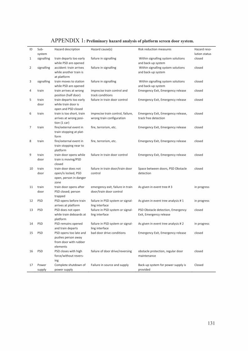
131
APPENDIX 1: Preliminary hazard analysis of platform screen door system.
ID Sub-system
Hazard description Hazard cause(s) Risk reduction measures Hazard reso-lution status
1 signalling train departs too early while PSD are opened
failure in signalling Within signalling system solutions and back-up system
closed
2 signalling accident: train arrives while another train is at platform
failure in signalling Within signalling system solutions and back-up system
closed
3 signalling train moves to station while PSD are opened
failure in signalling Within signalling system solutions and back-up system
closed
4 train train arrives at wrong position (half door)
imprecise train control and track conditions
Emergency Exit, Emergency release closed
5 train door
train departs too early while train door is open and PSD closed
failure in train door control Emergency Exit, Emergency release closed
6 train train is too short, train arrives at wrong posi-tion (1 car)
imprecise train control, failure, wrong train configuration
Emergency Exit, Emergency release, track free detection
closed
7 train fire/external event in train stopping at plat-form
fire, terrorism, etc. Emergency Exit, Emergency release closed
8 train fire/external event in train stopping near to platform
fire, terrorism, etc. Emergency Exit, Emergency release closed
9 train door
train door opens while train is moving/PSD closed
failure in train door control Emergency Exit, Emergency release closed
10 train door
train door does not open/is locked, PSD open, person in danger zone
failure in train door/train door control
Space between doors, PSD Obstacle detection
closed
11 train door
train door opens after PSD closed; person trapped
emergency exit, failure in train door/train door control
As given in event tree # 3 in progress
12 PSD PSD opens before train arrives at platform
failure in PSD system or signal-ling interface
As given in event tree analysis # 1 in progress
13 PSD PSD does not open while train deboards at platform
failure in PSD system or signal-ling interface
PSD Obstacle detection, Emergency Exit, Emergency release
closed
14 PSD PSD remains opened and train departs
failure in PSD system or signal-ling interface
As given in event tree analysis # 2 in progress
15 PSD PSD opens too late and pushes person away from door with rubber elements
bad door drive conditions Emergency Exit, Emergency release closed
16 PSD PSD closes with high force/without revers-ing
failure of door drive/reversing obstacle protection, regular door maintenance
closed
17 Power supply
Complete shutdown of power supply
Failure in source and supply Back-up system for power supply is provided
Closed


06 November 2013
To whom it may concern,
RE: Proof-Reading-Service.com Editorial Certification
This is to confirm that the document described below has been submitted to Proof-Reading-Service.com for editing and proofreading.
We certify that the editor has corrected the document, ensured consistency of the spelling, grammar and punctuation, and checked the format of the sub-headings, bibliographical references, tables, figures etc. The editor has further checked that the document is formatted according to the style guide supplied by the author. If no style guide was supplied, the editor has corrected the references in accordance with the style that appeared to be prevalent in the document and imposed internal consistency, at least, on the format. It is up to the author to accept, reject or respond to any changes, corrections, suggestions and recommendations made by the editor. This often involves the need to add or complete bibliographical references and respond to any comments made by the editor, in particular regarding clarification of the text or the need for further information or explanation. We are one of the largest proofreading and editing services worldwide for research documents, covering all academic areas including Engineering, Medicine, Physical and Biological Sciences, Social Sciences, Economics, Law, Management and the Humanities. All our editors are native English speakers and educated at least to Master’s degree level (many hold a PhD) with extensive university and scientific editorial experience. Document title: A Bayesian Network Methodology for Railway Risk, Safety and
Decision Support Author(s): Qamar Mahboob Format: British English Style guide: Harvard Particular comments: None


![METHODOLOGY FOR CLASSIFICATION SECTIONS OF RAILWAY … · 2019-05-22 · Northeast China railway network. The railway passenger stations have been classified in [3], using the method](https://img.pdfslide.net/doc/110x75/5f55671e6b977a412e6b9bef/methodology-for-classification-sections-of-railway-2019-05-22-northeast-china.jpg)