Embed Size (px)
Citation preview
10/31/08
A Before-After-Control-Impact Analysis for
Cornell University’s Lake Source Cooling Facility
Prepared by:
Upstate Freshwater Institute
P.O. Box 506
Syracuse, NY 13214
Sponsored by:
Cornell University
Department of Utilities and Energy Management
October 2008
10/31/08
2
1. Objective
The primary objective of this report is to determine if levels of three water quality
parameters (chlorophyll a, total phosphorus, turbidity) have shown statistically significant
changes in the southern portion of Cayuga Lake coincident in time with start-up of Cornell’s
Lake Source Cooling (LSC) facility. Statistical determinations are made based on a Before-
After-Control-Impact (BACI) design applied to in-lake monitoring data collected over the 1998 –
2005 interval.
2. Cayuga Lake and the Lake Source Cooling Facility
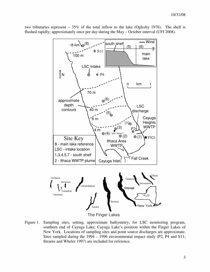
Cayuga Lake is the fourth easternmost of the New York Finger Lakes (Figure 1); it has
the largest surface area (172 km2) and the second largest volume (9.38 x 10
9 m
3) of this system
of lakes (Schaffner and Oglesby 1978). The lake is long (61.4 km along its major axis) and
narrow, extending along a north/south axis (Figure 1). Its stratification regime is warm
monomictic, stratifying strongly in summer, but complete ice cover has only rarely occurred
(Oglesby 1978). The lake’s large hypolimnion remains cold (e.g., < 5 ºC) through the summer.
The watershed area of this alkaline hardwater lake is ~ 1150 km2 (Oglesby 1978). Water exits
the basin through a single outlet at the northern end of the lake. The long-term average flushing
rate of the lake is slow, about 0.08 y-1
(Oglesby 1978, Effler et al. 1989). The City of Ithaca and
Cornell University are located at the southeastern end of Cayuga Lake.
Cayuga Lake is generally considered to be mesotrophic (e.g., Oglesby 1978). This
position is supported by available long-term measurements of the trophic state indicators of total
phosphorus (TP) and chlorophyll a (Chl) for the epilimnion in deep-water locations (UFI 2007).
Phytoplankton growth in the lake is phosphorus-limited (Oglesby 1978). Conditions in the
southern end of Cayuga Lake, particularly the southernmost 2 km with depths < 6 m (Figure 1;
designated the “shelf”), have generally been considered degraded relative to the deep-water
portions of the lake (Oglesby 1978). The occurrence of higher turbidity levels is a prominent
feature of this perceived degradation (e.g., Oglesby 1978). Total phosphorus concentrations
have routinely exceeded 20 µg·L-1
on the shelf (UFI 2003), the “guidance” value (i.e., open to
some regulatory discretion) for New York [New York State Department of Environmental
Conservation (NYSDEC) 1993] to protect recreational uses of lakes. Recently, NYSDEC added
this portion of the lake to the state’s list of water quality limited systems (as per section 303d of
the Federal Clean Water Act), which may be followed by a “total maximum daily load” (TMDL)
analysis.
The shelf receives a number of external inputs, including effluents from two domestic
waste treatment facilities (Ithaca WWTP and Cayuga Heights WWTP), spent cooling water from
Cornell’s Lake Source Cooling (LSC) facility, and inflows from the two largest tributaries of the
lake (Cayuga Inlet and Fall Creek; Figure 1). Average effluent flows for the two treatment
facilities are 0.3 and 0.07 m3·s
-1; the TP limit for these discharges is 1 mg·L
-1 (Great Lakes basin
standard). The annual average flow rate from the LSC facility has been about 0.7 m3·s
-1, which
is 8% of the total flow to the southern portion of Cayuga Lake. During the growing season (June
– September) tributary flow rates decrease and the average flow from LSC increases to 1.1
m3·s
-1. As a result, LSC contributes about 30% of the total inflow during June – September. The
10/31/08
3
two tributaries represent ~ 35% of the total inflow to the lake (Oglesby 1978). The shelf is
flushed rapidly; approximately once per day during the May – October interval (UFI 2008).
(7)
LSC
discharge
(1)
(2)
(3)
(4)
(5)
(6)
LSC Intake
Ithaca Area WWTP
Cayuga Heights WWTP
Fall CreekCayuga Inlet
Wind
(5) (6)
mainlake
south shelf
40 m
6 m
4 m
70 m
100 m
0 1km
approximate depth
contours
Site Key8 - main lake reference
LSC - intake location
1,3,4,5,7 - south shelf
2 - Ithaca WWTP plume
(8)~8 km
N
T921
“pile cluster”
P2
P4
S11
New York
The Finger Lakes
Conesus
Hemlock
Canadice
Honeoye
Canandaigua
Keuka
Seneca
Cayuga
Owasco
Skaneateles
Otisco
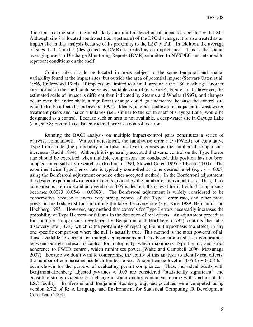
Figure 1. Sampling sites, setting, approximate bathymetry, for LSC monitoring program,
southern end of Cayuga Lake; Cayuga Lake’s position within the Finger Lakes of
New York. Locations of sampling sites and point source discharges are approximate.
Sites sampled during the 1994 – 1996 environmental impact study (P2, P4 and S11;
Stearns and Wheler 1997) are included for reference.
10/31/08
4
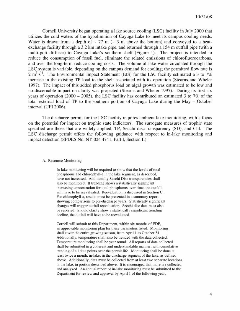
Cornell University began operating a lake source cooling (LSC) facility in July 2000 that
utilizes the cold waters of the hypolimnion of Cayuga Lake to meet its campus cooling needs.
Water is drawn from a depth of ~ 77 m (~ 3 m above the bottom) and conveyed to a heat-
exchange facility through a 3.2 km intake pipe, and returned through a 154 m outfall pipe (with a
multi-port diffuser) to Cayuga Lake’s southern shelf (Figure 1). The project is intended to
reduce the consumption of fossil fuel, eliminate the related emissions of chlorofluorocarbons,
and over the long-term reduce cooling costs. The volume of lake water circulated through the
LSC system is variable, depending on the campus demand for cooling; the permitted flow rate is
2 m3·s
-1. The Environmental Impact Statement (EIS) for the LSC facility estimated a 3 to 7%
increase in the existing TP load to the shelf associated with its operation (Stearns and Wheler
1997). The impact of this added phosphorus load on algal growth was estimated to be low and
no discernable impact on clarity was projected (Stearns and Wheler 1997). During its first six
years of operation (2000 – 2005), the LSC facility has contributed an estimated 3 to 7% of the
total external load of TP to the southern portion of Cayuga Lake during the May – October
interval (UFI 2006).
The discharge permit for the LSC facility requires ambient lake monitoring, with a focus
on the potential for impact on trophic state indicators. The surrogate measures of trophic state
specified are those that are widely applied, TP, Secchi disc transparency (SD), and Chl. The
LSC discharge permit offers the following guidance with respect to in-lake monitoring and
impact detection (SPDES No. NY 024 4741, Part I, Section II):
A. Resource Monitoring
In-lake monitoring will be required to show that the levels of total
phosphorus and chlorophyll-a in the lake segment, as described,
have not increased. Additionally Secchi Disc transparencies shall
also be monitored. If trending shows a statistically significant
increasing concentration for total phosphorus over time, the outfall
will have to be reevaluated. Reevaluation is discussed in Section C.
For chlorophyll-a, results must be presented in a summary report
showing comparisons to pre-discharge years. Statistically significant
changes will trigger outfall reevaluation. Secchi disc data must also
be reported. Should clarity show a statistically significant trending
decline, the outfall will have to be reevaluated.
Cornell will submit to this Department, within six months of EDP,
an approvable monitoring plan for these parameters listed. Monitoring
shall cover the entire growing season, from April 1 to October 31.
Additionally, temperature shall also be trended with the data collected.
Temperature monitoring shall be year round. All reports of data collected
shall be submitted in a coherent and understandable manner, with cumulative
trending of all data points over the permit life. Monitoring shall be done at
least twice a month, in-lake, in the discharge segment of the lake, as defined
above. Additionally, data must be collected from at least two separate locations
in the lake, in portion described above. It is encouraged that more are collected
and analyzed. An annual report of in-lake monitoring must be submitted to the
Department for review and approval by April 1 of the following year.
10/31/08
5
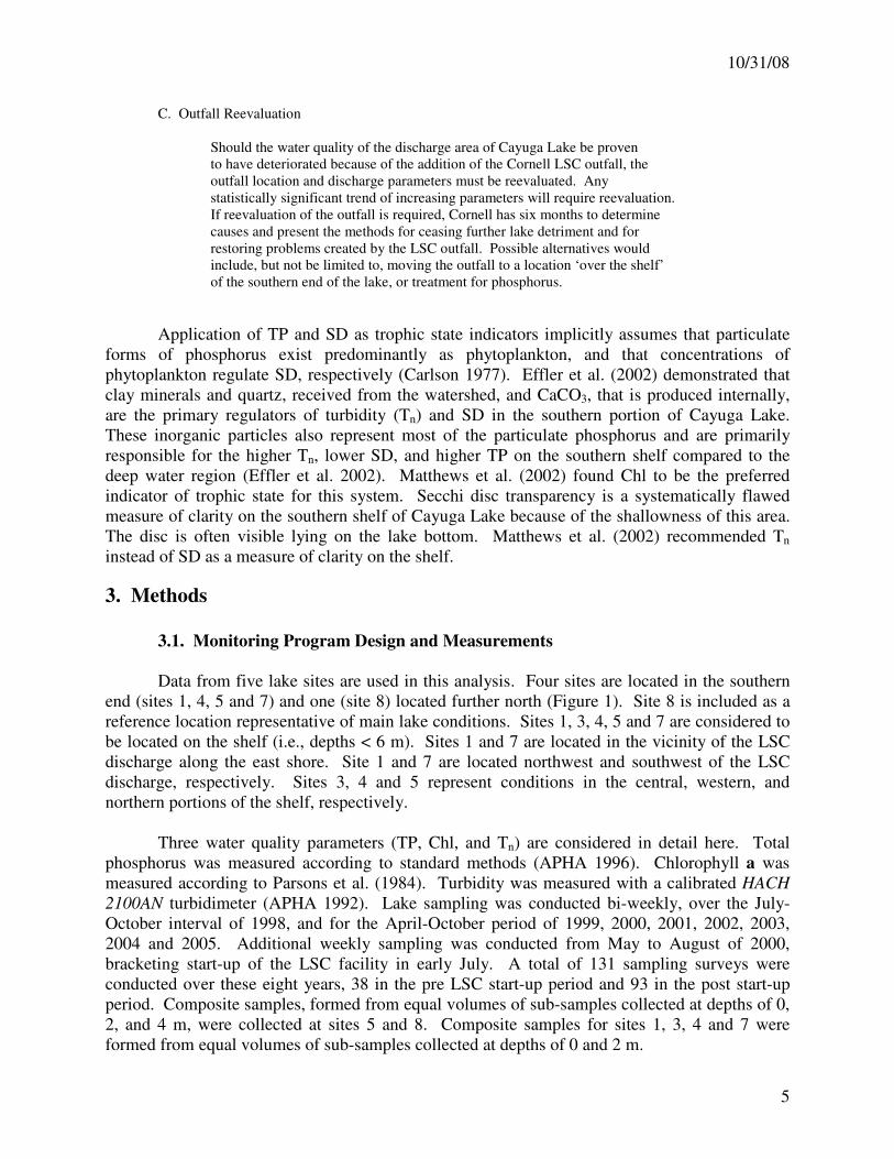
C. Outfall Reevaluation
Should the water quality of the discharge area of Cayuga Lake be proven
to have deteriorated because of the addition of the Cornell LSC outfall, the
outfall location and discharge parameters must be reevaluated. Any
statistically significant trend of increasing parameters will require reevaluation.
If reevaluation of the outfall is required, Cornell has six months to determine
causes and present the methods for ceasing further lake detriment and for
restoring problems created by the LSC outfall. Possible alternatives would
include, but not be limited to, moving the outfall to a location ‘over the shelf’
of the southern end of the lake, or treatment for phosphorus.
Application of TP and SD as trophic state indicators implicitly assumes that particulate
forms of phosphorus exist predominantly as phytoplankton, and that concentrations of
phytoplankton regulate SD, respectively (Carlson 1977). Effler et al. (2002) demonstrated that
clay minerals and quartz, received from the watershed, and CaCO3, that is produced internally,
are the primary regulators of turbidity (Tn) and SD in the southern portion of Cayuga Lake.
These inorganic particles also represent most of the particulate phosphorus and are primarily
responsible for the higher Tn, lower SD, and higher TP on the southern shelf compared to the
deep water region (Effler et al. 2002). Matthews et al. (2002) found Chl to be the preferred
indicator of trophic state for this system. Secchi disc transparency is a systematically flawed
measure of clarity on the southern shelf of Cayuga Lake because of the shallowness of this area.
The disc is often visible lying on the lake bottom. Matthews et al. (2002) recommended Tn
instead of SD as a measure of clarity on the shelf.
3. Methods
3.1. Monitoring Program Design and Measurements
Data from five lake sites are used in this analysis. Four sites are located in the southern
end (sites 1, 4, 5 and 7) and one (site 8) located further north (Figure 1). Site 8 is included as a
reference location representative of main lake conditions. Sites 1, 3, 4, 5 and 7 are considered to
be located on the shelf (i.e., depths < 6 m). Sites 1 and 7 are located in the vicinity of the LSC
discharge along the east shore. Site 1 and 7 are located northwest and southwest of the LSC
discharge, respectively. Sites 3, 4 and 5 represent conditions in the central, western, and
northern portions of the shelf, respectively.
Three water quality parameters (TP, Chl, and Tn) are considered in detail here. Total
phosphorus was measured according to standard methods (APHA 1996). Chlorophyll a was
measured according to Parsons et al. (1984). Turbidity was measured with a calibrated HACH
2100AN turbidimeter (APHA 1992). Lake sampling was conducted bi-weekly, over the July-
October interval of 1998, and for the April-October period of 1999, 2000, 2001, 2002, 2003,
2004 and 2005. Additional weekly sampling was conducted from May to August of 2000,
bracketing start-up of the LSC facility in early July. A total of 131 sampling surveys were
conducted over these eight years, 38 in the pre LSC start-up period and 93 in the post start-up
period. Composite samples, formed from equal volumes of sub-samples collected at depths of 0,
2, and 4 m, were collected at sites 5 and 8. Composite samples for sites 1, 3, 4 and 7 were
formed from equal volumes of sub-samples collected at depths of 0 and 2 m.
10/31/08
6
Precision of sampling, sample handling and laboratory analyses was assessed by a
program of field replicates. Samples for laboratory analyses were collected in triplicate at site 1
on each sampling day. Triplicate samples were collected at one other station each monitoring
trip. This station was rotated each sampling trip through the field season. Precision was high for
the triplicate sampling/measurement program, as represented by the average values of the
coefficient of variation for the six study years (Table 1). Variability was similar for the three
parameters considered here (Table 1). The magnitude of uncertainty associated with these
measurements should be recognized when interpreting the analyses that follow.
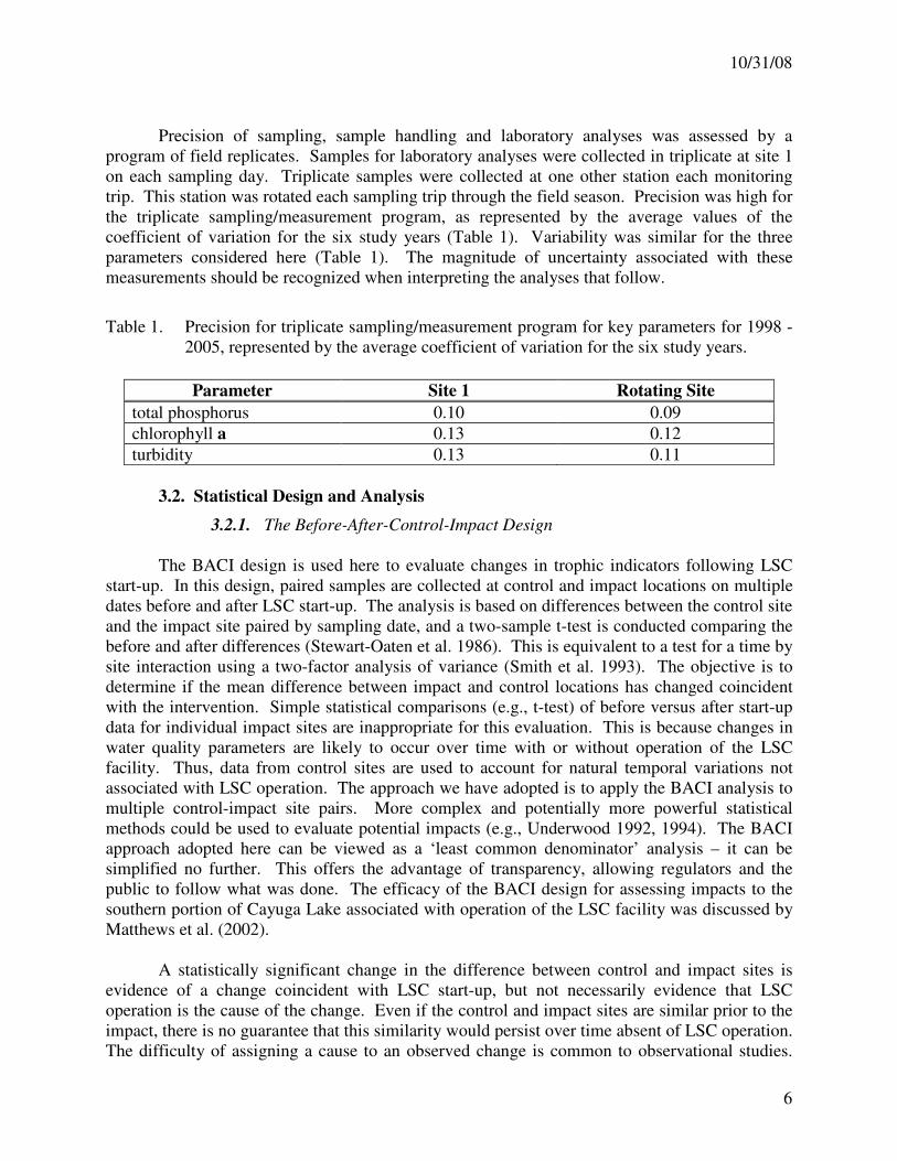
Table 1. Precision for triplicate sampling/measurement program for key parameters for 1998 -
2005, represented by the average coefficient of variation for the six study years.
Parameter Site 1 Rotating Site
total phosphorus 0.10 0.09
chlorophyll a 0.13 0.12
turbidity 0.13 0.11
3.2. Statistical Design and Analysis
3.2.1. The Before-After-Control-Impact Design
The BACI design is used here to evaluate changes in trophic indicators following LSC
start-up. In this design, paired samples are collected at control and impact locations on multiple
dates before and after LSC start-up. The analysis is based on differences between the control site
and the impact site paired by sampling date, and a two-sample t-test is conducted comparing the
before and after differences (Stewart-Oaten et al. 1986). This is equivalent to a test for a time by
site interaction using a two-factor analysis of variance (Smith et al. 1993). The objective is to
determine if the mean difference between impact and control locations has changed coincident
with the intervention. Simple statistical comparisons (e.g., t-test) of before versus after start-up
data for individual impact sites are inappropriate for this evaluation. This is because changes in
water quality parameters are likely to occur over time with or without operation of the LSC
facility. Thus, data from control sites are used to account for natural temporal variations not
associated with LSC operation. The approach we have adopted is to apply the BACI analysis to
multiple control-impact site pairs. More complex and potentially more powerful statistical
methods could be used to evaluate potential impacts (e.g., Underwood 1992, 1994). The BACI
approach adopted here can be viewed as a ‘least common denominator’ analysis – it can be
simplified no further. This offers the advantage of transparency, allowing regulators and the
public to follow what was done. The efficacy of the BACI design for assessing impacts to the
southern portion of Cayuga Lake associated with operation of the LSC facility was discussed by
Matthews et al. (2002).
A statistically significant change in the difference between control and impact sites is
evidence of a change coincident with LSC start-up, but not necessarily evidence that LSC
operation is the cause of the change. Even if the control and impact sites are similar prior to the
impact, there is no guarantee that this similarity would persist over time absent of LSC operation.
The difficulty of assigning a cause to an observed change is common to observational studies.
10/31/08
7
Discovering the cause of any observed changes in trophic indicators in the southern end of
Cayuga Lake is particularly complicated because of the potential for simultaneous changes in
multiple drivers not associated with LSC start-up and operation. Matthews et al. (2002)
discussed a number of these potentially confounding factors including: (1) natural variation in
meteorological conditions, (2) changes in treatment at wastewater treatment plants, and (3) the
uncertain effects of zebra mussel populations.
It is also important to note that statistical significance is not equivalent to biological
significance (Scheiner and Gurevitch 2001). Large studies conducted on populations that vary
little may detect very small, biologically unimportant effects as significant. Conversely,
biologically meaningful effects can go undetected if sample sizes are small or natural spatial or
temporal variability is high. Sample sizes for this study are large, 38 and 93 for the pre and post
start-up intervals, respectively. The three variables of interest (Chl, TP and Tn) have exhibited
substantial variability on the southern shelf of Cayuga Lake, both among sites and over time at
individual sites (Matthews et al. 2002, UFI 1999-2007). Power analyses conducted by Matthews
et al. (2002) on pre start-up data established that the BACI analysis would detect a 30% change
in Chl with a probability of 0.7 at α = 0.05. The probability of detecting a 30% change in Chl
increases to about 0.8 if evaluated at α = 0.10. Similar results were obtained for TP and Tn (UFI,
unpublished results). Thus, the statistical design adopted here is appropriate for the detection of
changes on the order of about 30% or greater, though substantially smaller effects will likely be
judged statistically insignificant. These power analyses were conducted on uncorrected p-values
and are not representative of the lower statistical power that results from the Bonferroni or
Benjamini and Hochberg (1995) adjustments for multiple comparisons.
3.2.2. Outlier Analysis
An outlier analysis (Section 6) was performed on untransformed TP, Chl, and Tn data
using Grubbs’s test statistic for outliers (Sokal and Rohlf 1995). Grubbs’s test statistic is (Y1 –
Y)/s, where Y1 is the suspected outlier, Y is the sample mean, and s is the sample standard
deviation. Critical values for Grubbs’s test statistic are presented in Sokal and Rohlf (1995).
This test was performed on a site-by-site basis for both the before LSC and after LSC periods.
Deviations from the mean found to be significant at a two-tailed probability of 0.05 were
identified and the veracity of these measurements was investigated using other supporting
information. Statistical outliers that could not be explained with available data were identified,
and the BACI analysis was conducted both with and without these data points.
3.2.3. Selection of Impact and Control Sites and Significance Levels
Application of the BACI design begins with a priori selection of suitable impact and
control sites. Impact sites should be located within the area potentially affected by LSC
operation. Not surprisingly, potential impacts are most likely in the immediate vicinity (e.g.,
diffuser “mixing zone”) of the LSC discharge (Stearns and Wheler 1997). Further, there is some
limited information that suggests a predominant counterclockwise flow pattern in the southern
end of Cayuga Lake, particularly following major runoff events (Oglesby 1978). This flow
pattern is expected to cause the LSC discharge to move to the north, in the direction of site 1
(Figure 1). Further, model projections included in the Draft Environmental Impact Statement
(Stearns and Wheler 1997) predicted that the LSC discharge would usually move in a northerly
10/31/08
8
direction, making site 1 the most likely location for detection of impacts associated with LSC.
Although site 7 is located southwest (i.e., upstream) of the LSC discharge, it is also treated as an
impact site in this analysis because of its proximity to the LSC outfall. In addition, the average
of sites 1, 3, 4 and 5 (designated as DMR) is treated as an impact area. This is the spatial
averaging used in Discharge Monitoring Reports (DMR) submitted to NYSDEC and intended to
represent conditions on the shelf.
Control sites should be located in areas subject to the same temporal and spatial
variability found at the impact sites, but outside the area of potential impact (Stewart-Oaten et al.
1986, Underwood 1994). If impacts are limited to a small area near the LSC discharge, another
site located on the shelf could serve as a suitable control (e.g., site 4; Figure 1). If, however, the
estimated scale of impact is different than indicated by Stearns and Wheler (1997), and changes
occur over the entire shelf, a significant change could go undetected because the control site
would also be affected (Underwood 1994). Ideally, another shallow area adjacent to wastewater
treatment plants and major tributaries (i.e., similar to the south shelf of Cayuga Lake) would be
designated as a control. Because such an area is not available, a deep-water site in Cayuga Lake
(e.g., site 8; Figure 1) is also considered here as a control location.
Running the BACI analysis on multiple impact-control pairs constitutes a series of
pairwise comparisons. Without adjustment, the familywise error rate (FWER), or cumulative
Type-I error rate (the probability of a false positive) increases as the number of comparisons
increases (Kuehl 1994). Although it is generally accepted that some control on the Type I error
rate should be exercised when multiple comparisons are conducted, this position has not been
adopted universally by researchers (Rothman 1990, Stewart-Oaten 1995, O’Keefe 2003). The
experimentwise Type-I error rate is typically controlled at some desired level (e.g., α = 0.05)
using the Bonferroni adjustment or some other accepted method. In the Bonferroni adjustment,
the desired experimentwise error rate α is divided by the number of individual tests. Thus, if six
comparisons are made and an overall α = 0.05 is desired, the α-level for individual comparisons
becomes 0.0083 (0.05/6 = 0.0083). The Bonferroni adjustment is widely considered to be
conservative because it exerts very strong control of the Type-I error rate, and other more
powerful methods exist for controlling the false discovery rate (e.g., Rice 1989, Benjamini and
Hochberg 1995). However, any method that controls for Type I errors necessarily increases the
probability of Type II errors, or failures in the detection of real effects. An adjustment procedure
for multiple comparisons developed by Benjamini and Hochberg (1995) controls the false
discovery rate (FDR), which is the probability of rejecting the null hypothesis (no effect) in any
one specific comparison where the null is actually true. This method is the most powerful of all
those available to correct for multiple comparisons and has been promoted as a compromise
between outright refusal to control for multiplicity, which maximizes Type I error, and strict
adherence to FWER control, which minimizes power (Waite and Campbell 2006, Matsunaga
2007). Because we don’t want to compromise the ability of this analysis to identify real effects,
the number of comparisons has been limited to six. A significance level of 0.05 (α = 0.05) has
been chosen for the purpose of evaluating permit compliance. Thus, individual t-tests with
Benjamini-Hochberg adjusted p-values < 0.05 are considered “statistically significant” and
constitute strong evidence of a change in water quality coincident in time with start-up of the
LSC facility. Bonferroni and Benjamini-Hochberg adjusted p-values were computed using
version 2.7.2 of R: A Language and Environment for Statistical Computing (R Development
Core Team 2008).
10/31/08
9
Impact-control site pairings for the BACI analysis were not determined prior to collection
and preliminary analysis of the data. Therefore, we cannot eliminate the possibility that selection
of the pairwise comparisons was biased by knowledge of the results. This issue bears directly on
the appropriate interpretation of the p-values presented. In the interest of transparency, both
adjusted and unadjusted p-values are presented in this report. However, the unadjusted p-values
are confounded by the fact that the pairwise comparisons presented here are a small subset of
those actually conducted. Approximately 20 individual pairwise comparisons were conducted at
α = 0.05, resulting in a probability of 0.64 that at least one statistically significant (unadjusted
p<0.05) difference would be detected by chance alone. This rate of false detection would be
considered unacceptably high in a scientific study. Thus, Benjamini-Hochberg adjusted p-values
are presented as the most appropriate indicator of statistically significant changes.
Based on careful consideration of the issues outlined above, the New York State
Department of Environmental Conservation and Cornell University have selected seven impact-
control pairs for the BACI analysis: (1) impact—site 1, control—site 4, (2) impact—site 1,
control—site 8, (3) impact—site 7, control—site 4, (4) impact—site 7, control—site 8, (5)
impact—site 4, control—site 8, (6) impact—site 5, control—site 4, and (7) DMR—site 8. These
seven pairings allow for the testing of a number of hypotheses related to potential changes in
trophic indicators in southern Cayuga Lake following LSC start-up. Pairings No. 1 and No. 3
provide tests of whether or not levels of TP, Chl and Tn increased disproportionately at sites 1
and 7 compared to site 4 following LSC start-up. If, however, site 4 was also impacted, this test
could fail to detect a substantial change in water quality. Pairings No. 2 and 4 overcome this
problem by using site 8, which is located well beyond the zone of influence of the LSC
discharge, as the control. If any of the first four pairings produce a statistically significant result,
pairings No. 5 and 6 become important as checks for consistency and for defining the spatial
extent of the impact. Pairing No. 7 compares water quality changes on the shelf relative to those
at the deep water reference site 8. Adjustments for multiple comparisons were not applied to the
DMR-site 8 pairing because this test was considered to be chosen a priori. Although water
quality data continued to be collected through 2008, only data collected through 2005 is included
in this analysis because of potentially confounding effects related to a 50% reduction in TP
loading from the Ithaca Area Wastewater Treatment Plant beginning in 2006.
3.2.4. Assumptions of Statistical Tests
Values for TP (µg·L-1
), Chl (µg·L-1
) and Tn (NTU) were determined from samples
collected on the same day for replicate surveys conducted before and after start-up of the LSC
facility. The data were log-transformed to achieve additivity and reduce autocorrelation
(Stewart-Oaten et al. 1986) and differences (∆) were calculated between the values at impact and
control locations for each sampling date. Statistical significance is determined from two-tailed
Welch t-tests comparing the before and after differences for the various control-impact pairs.
STATISTICA version 6 (data analysis software system; StatSoft, Inc. 2003) was used for
statistical analyses.
The two-sample t-test conducted on the before and after differences is subject to the usual
assumptions for such a test: the observations (differences) are assumed independent, and the
sample sizes are assumed large enough so that the distribution of the mean differences (before
10/31/08
10
and after periods) is approximately normally distributed. Variances of the differences in the two
time periods need not be assumed equal if the Welch t-test (Snedecor and Cochran 1980) is used.
The normality assumption is likely satisfied by the data typically encountered in a BACI study
unless numerous zeros are present (as may occur for abundance data). Applying a logarithmic
transformation, which is a common practice with environmental data (Eberhardt and Thomas
1991, Stewart-Oaten et al. 1992, Osenberg et al. 1994), reduces skewness of the data prior to
calculating differences, and taking differences still further diminishes skewness (Stewart-Oaten
et al. 1992). Sample sizes for both the before and after periods exceed 30 in this study;
consequently, the Central Limit Theorem further contributes to approximate normality of the
distribution of the mean differences. If the normality assumption is problematic, the Mann-
Whitney (also called Wilcoxon) non-parametric two-sample test or a randomization test
(Carpenter et al. 1989) can be used in place of the Welch t-test. Although these alternatives do
not invoke a normality assumption, they do require the other assumptions of the Welch t-test
(Stewart-Oaten et al. 1992). Because the normality assumption was not satisfied for all of the
impact-control distributions (Appendix 1), Mann-Whitney tests were conducted for all impact-
control pairs. The Mann-Whitney tests yielded results consistent with the Welch t-tests, and no
significant (Benjamini & Hochberg adjusted p < 0.05) pre-post differences were observed (see
Appendix 4).
The independence assumption is likely more of a concern than the normality assumption
because of possible serial correlation of the differences over the sampling times. The effect of
positive serial correlation is to inflate the Type I error rate of the test. In other words, positive
serial correlation will make it more likely to detect a LSC effect that does not exist. Stewart-
Oaten et al. (1986) emphasize that it is the differences that must be uncorrelated, not the
observations over time at each individual sampling station. Serial correlation of the differences
is not expected to be nearly as strong as serial correlation in the observations obtained at each
individual site. Even if serial correlation is found to be statistically significant, conclusions of
the BACI test remain valid if the serial correlation is small; e.g., lag-1 r < 0.3 (Stewart-Oaten et
al. 1986).
Another assumption of the BACI analysis is 'additivity' of time and location effects.
Violation of this assumption may cause the BACI test to lose power because the differences are
highly variable or inflate the actual Type I error of the test (Stewart-Oaten et al. 1986, Smith et
al. 1993). Stewart-Oaten et al. (1986) suggest employing Tukey's (1949) test for non-additivity,
although Smith et al. (1993) note that the test for additivity is sensitive to serial correlation. If
non-additivity exists, a log-transformation often diminishes or eliminates the problem. Stewart-
Oaten et al. (1992) discuss more details of the additivity assumption. After log transformation
and differencing (impact-control), the data were checked against the assumptions for a Welch t-
test (normality, temporal independence, additivity). Evaluations of the normality, independence,
and additivity assumptions are presented in Appendixes 1, 2, and 3, respectively.
3.2.5. Calculation and Interpretation of Effect Size
For the BACI design, the test for an impact associated with LSC start-up is an interaction
test: does the mean difference between the control and impact site before LSC start-up differ
from the mean difference after start-up? Because the key test is one of interaction, defining a
readily interpretable effect size is more difficult than when the test is a comparison of means
10/31/08
11
(rather than mean differences). The rationale for choosing and interpreting effect size is as
follows. In the Before period, suppose the mean of the control site is x, and that the mean of the
impact site is a% higher, (1+a)x. Both the control and impact site means increase b% in the
After period, so the control site has mean (1+b)x, and the impact site has mean (1+a)(1+b)x.
This b% increase for both control and impact sites is consistent with additivity on a log-
transformed scale. If an impact is present, suppose it further increases the mean of the impact
site in the After period by an additional c%, so the impact site mean is (1+a)(1+b)(1+c)x. On the
log-transformed scale, the difference in means in the Before period is then log(x)log[(1+a)x] =
log[x/(1+a)x] = log[1/(1+a)], and the difference in means in the After period is log[(1+b)x] –
log[(1+a)(1+b)(1+c)x] = -log[1/(1+a)(1+c)]. Finally, the interaction test would evaluate the
difference of the differences in the Before and After period, resulting in -log[1/(1+a)(1+c)] –
log[(1/(1+a)] = -log[1/(1+c)]. Thus, the effect size c is the percent increase in a variable
associated with the impact. This formulation of the effect size is consistent with a multiplicative
effects model that motivates analysis on the logarithmic scale.
The calculation and interpretation of effect size is illustrated here using a hypothetical
example. Suppose that in the Before period the mean chlorophyll a concentration of the control
site (x) is 5 µg·L-1
and the mean chlorophyll a concentration of the impact site (y) is 20% higher,
y = (1+ 0.20)x = 6 µg·L-1
. Both the control and impact site means increase 10% in the After
period, so the control site has mean (1+0.10)5 µg·L-1
= 5.5 µg·L-1
, and the impact site has mean
(1+0.20)(1+0.10)5 µg·L-1
= 6.6 µg·L-1
. Suppose that a perturbation in the After period causes the
mean chlorophyll a concentration of the impact site to increase by an additional 20%, so the
impact site mean is (1+0.20)(1+0.10)(1+0.20)5 µg·L-1
= 7.92 µg·L-1
. In the BACI analysis, we
evaluate the increase at the impact site over and above any increases that also occurred at the
control site. On the log-transformed scale this increase is log(7.92 µg·L-1
) – log(6.6 µg·L-1
) =
0.0792. We can see that this is equivalent to the formulation of effect size described above,
-log[1/(1+0.20)] = 0.0792. Thus, the effect size c can be determined by solving 0.0792 =
-log[1/(1+c)] for c, which yields c = 0.20.
4. Simple Before-After Comparison of Mean Values
A simple comparison of mean values for the pre and post LSC start-up intervals is
presented here as a way to characterize water quality changes in the southern portion of Cayuga
Lake. This analysis is presented outside of the BACI results (Section 7) because it is not an
appropriate method for assessing potential impacts associated with the LSC facility. Changes in
water quality would be expected to occur with or without LSC operation. In fact, chlorophyll a
(Chl) concentrations decreased 35% from 1994 – 1996 to 1998 – 1999 in the absence of LSC or
any other documented perturbation (UFI 2007). Furthermore, total phosphorus (TP) and Chl
concentrations increased on the southern shelf in 2006 despite a 50% decrease in TP loading
from IAWWTP. Thus, the simple comparison of mean values presented here should be
interpreted as a snapshot in time of a complex ecosystem and not as a cause and effect analysis.
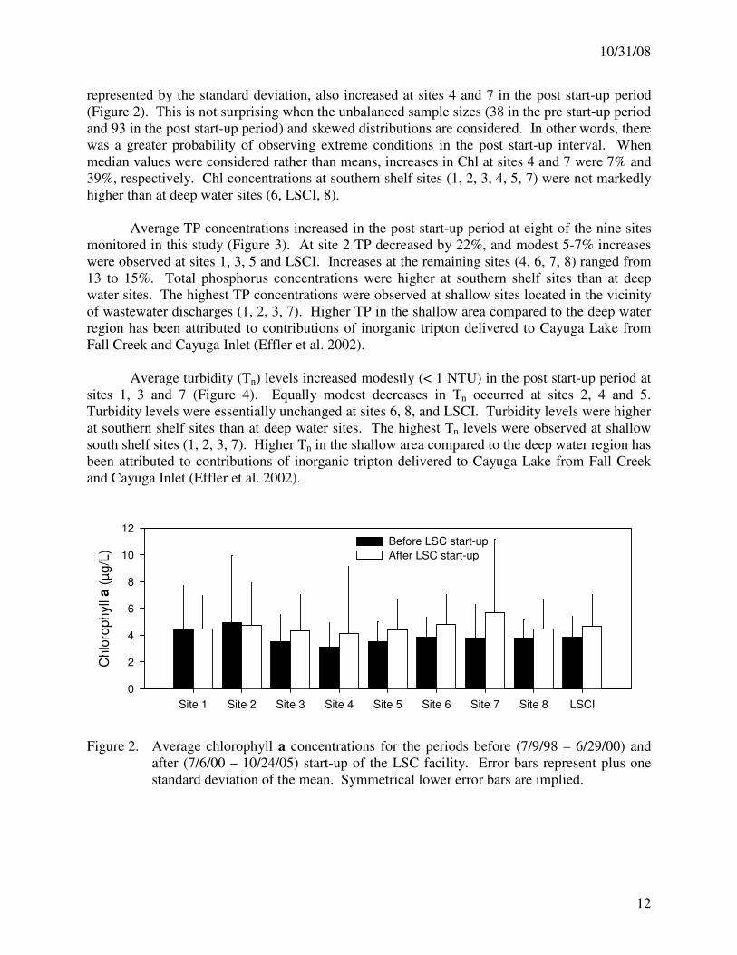
Average chlorophyll a concentrations increased in the post start-up period at eight of the
nine sites monitored in this study (Figure 2). At site 2 Chl decreased by 4% and the increase at
site 1 was just 1%. Increases at the remaining sites (3, 4, 5, 6, 7, 8, LSCI) ranged from 16 to
49%. The largest increases occurred at site 4 (31%) and site 7 (49%). Temporal variability, as
10/31/08
12
represented by the standard deviation, also increased at sites 4 and 7 in the post start-up period
(Figure 2). This is not surprising when the unbalanced sample sizes (38 in the pre start-up period
and 93 in the post start-up period) and skewed distributions are considered. In other words, there
was a greater probability of observing extreme conditions in the post start-up interval. When
median values were considered rather than means, increases in Chl at sites 4 and 7 were 7% and
39%, respectively. Chl concentrations at southern shelf sites (1, 2, 3, 4, 5, 7) were not markedly
higher than at deep water sites (6, LSCI, 8).
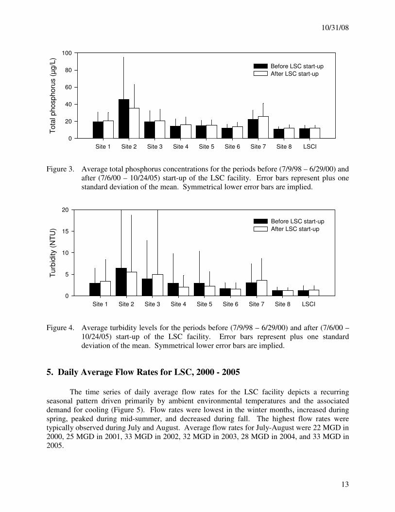
Average TP concentrations increased in the post start-up period at eight of the nine sites
monitored in this study (Figure 3). At site 2 TP decreased by 22%, and modest 5-7% increases
were observed at sites 1, 3, 5 and LSCI. Increases at the remaining sites (4, 6, 7, 8) ranged from
13 to 15%. Total phosphorus concentrations were higher at southern shelf sites than at deep
water sites. The highest TP concentrations were observed at shallow sites located in the vicinity
of wastewater discharges (1, 2, 3, 7). Higher TP in the shallow area compared to the deep water
region has been attributed to contributions of inorganic tripton delivered to Cayuga Lake from
Fall Creek and Cayuga Inlet (Effler et al. 2002).
Average turbidity (Tn) levels increased modestly (< 1 NTU) in the post start-up period at
sites 1, 3 and 7 (Figure 4). Equally modest decreases in Tn occurred at sites 2, 4 and 5.
Turbidity levels were essentially unchanged at sites 6, 8, and LSCI. Turbidity levels were higher
at southern shelf sites than at deep water sites. The highest Tn levels were observed at shallow
south shelf sites (1, 2, 3, 7). Higher Tn in the shallow area compared to the deep water region has
been attributed to contributions of inorganic tripton delivered to Cayuga Lake from Fall Creek
and Cayuga Inlet (Effler et al. 2002).
Site 1 Site 2 Site 3 Site 4 Site 5 Site 6 Site 7 Site 8 LSCI
Chlo
rophyll
a (
µg/L
)
0
2
4
6
8
10
12Before LSC start-up
After LSC start-up
Figure 2. Average chlorophyll a concentrations for the periods before (7/9/98 – 6/29/00) and
after (7/6/00 – 10/24/05) start-up of the LSC facility. Error bars represent plus one
standard deviation of the mean. Symmetrical lower error bars are implied.
10/31/08
13
Site 1 Site 2 Site 3 Site 4 Site 5 Site 6 Site 7 Site 8 LSCI
Tota
l phosp
horu
s (
µg/L
)
0
20
40
60
80
100
Before LSC start-up
After LSC start-up
Figure 3. Average total phosphorus concentrations for the periods before (7/9/98 – 6/29/00) and
after (7/6/00 – 10/24/05) start-up of the LSC facility. Error bars represent plus one
standard deviation of the mean. Symmetrical lower error bars are implied.
Site 1 Site 2 Site 3 Site 4 Site 5 Site 6 Site 7 Site 8 LSCI
Turb
idity (
NT
U)
0
5
10
15
20
Before LSC start-up
After LSC start-up
Figure 4. Average turbidity levels for the periods before (7/9/98 – 6/29/00) and after (7/6/00 –
10/24/05) start-up of the LSC facility. Error bars represent plus one standard
deviation of the mean. Symmetrical lower error bars are implied.
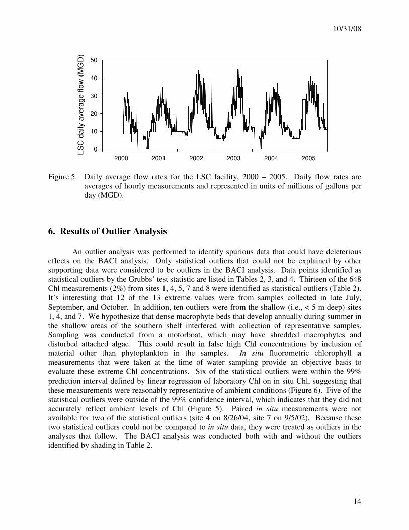
5. Daily Average Flow Rates for LSC, 2000 - 2005
The time series of daily average flow rates for the LSC facility depicts a recurring
seasonal pattern driven primarily by ambient environmental temperatures and the associated
demand for cooling (Figure 5). Flow rates were lowest in the winter months, increased during
spring, peaked during mid-summer, and decreased during fall. The highest flow rates were
typically observed during July and August. Average flow rates for July-August were 22 MGD in
2000, 25 MGD in 2001, 33 MGD in 2002, 32 MGD in 2003, 28 MGD in 2004, and 33 MGD in
2005.
10/31/08
14
2000 2001 2002 2003 2004 2005
LS
C d
aily
avera
ge flo
w (
MG
D)
0
10
20
30
40
50
Figure 5. Daily average flow rates for the LSC facility, 2000 – 2005. Daily flow rates are
averages of hourly measurements and represented in units of millions of gallons per
day (MGD).
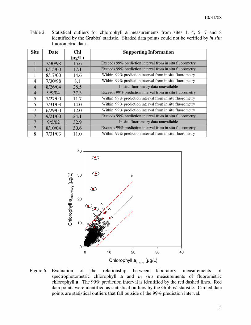
6. Results of Outlier Analysis
An outlier analysis was performed to identify spurious data that could have deleterious
effects on the BACI analysis. Only statistical outliers that could not be explained by other
supporting data were considered to be outliers in the BACI analysis. Data points identified as
statistical outliers by the Grubbs’ test statistic are listed in Tables 2, 3, and 4. Thirteen of the 648
Chl measurements (2%) from sites 1, 4, 5, 7 and 8 were identified as statistical outliers (Table 2).
It’s interesting that 12 of the 13 extreme values were from samples collected in late July,
September, and October. In addition, ten outliers were from the shallow (i.e., < 5 m deep) sites
1, 4, and 7. We hypothesize that dense macrophyte beds that develop annually during summer in
the shallow areas of the southern shelf interfered with collection of representative samples.
Sampling was conducted from a motorboat, which may have shredded macrophytes and
disturbed attached algae. This could result in false high Chl concentrations by inclusion of
material other than phytoplankton in the samples. In situ fluorometric chlorophyll a
measurements that were taken at the time of water sampling provide an objective basis to
evaluate these extreme Chl concentrations. Six of the statistical outliers were within the 99%
prediction interval defined by linear regression of laboratory Chl on in situ Chl, suggesting that
these measurements were reasonably representative of ambient conditions (Figure 6). Five of the
statistical outliers were outside of the 99% confidence interval, which indicates that they did not
accurately reflect ambient levels of Chl (Figure 5). Paired in situ measurements were not
available for two of the statistical outliers (site 4 on 8/26/04, site 7 on 9/5/02). Because these
two statistical outliers could not be compared to in situ data, they were treated as outliers in the
analyses that follow. The BACI analysis was conducted both with and without the outliers
identified by shading in Table 2.
10/31/08
15
Table 2. Statistical outliers for chlorophyll a measurements from sites 1, 4, 5, 7 and 8
identified by the Grubbs’ statistic. Shaded data points could not be verified by in situ
fluorometric data.
Site Date Chl
(µg/L)
Supporting Information
1 7/30/98 15.6 Exceeds 99% prediction interval from in situ fluorometry
1 6/15/00 17.1 Exceeds 99% prediction interval from in situ fluorometry
1 8/17/00 14.6 Within 99% prediction interval from in situ fluorometry
4 7/30/98 8.1 Within 99% prediction interval from in situ fluorometry
4 8/26/04 28.5 In situ fluorometry data unavailable
4 9/9/04 37.3 Exceeds 99% prediction interval from in situ fluorometry
5 7/27/00 11.7 Within 99% prediction interval from in situ fluorometry
5 7/31/03 14.0 Within 99% prediction interval from in situ fluorometry
7 6/29/00 12.0 Within 99% prediction interval from in situ fluorometry
7 9/21/00 24.1 Exceeds 99% prediction interval from in situ fluorometry
7 9/5/02 32.9 In situ fluorometry data unavailable
7 8/10/04 30.6 Exceeds 99% prediction interval from in situ fluorometry
8 7/31/03 11.0 Within 99% prediction interval from in situ fluorometry
Chlorophyll ain situ
(µg/L)
0 10 20 30 40
Chlo
rophyll
ala
bora
tory (
µg/L
)
0
10
20
30
40
Figure 6. Evaluation of the relationship between laboratory measurements of
spectrophotometric chlorophyll a and in situ measurements of fluorometric
chlorophyll a. The 99% prediction interval is identified by the red dashed lines. Red
data points were identified as statistical outliers by the Grubbs’ statistic. Circled data
points are statistical outliers that fall outside of the 99% prediction interval.
10/31/08
16
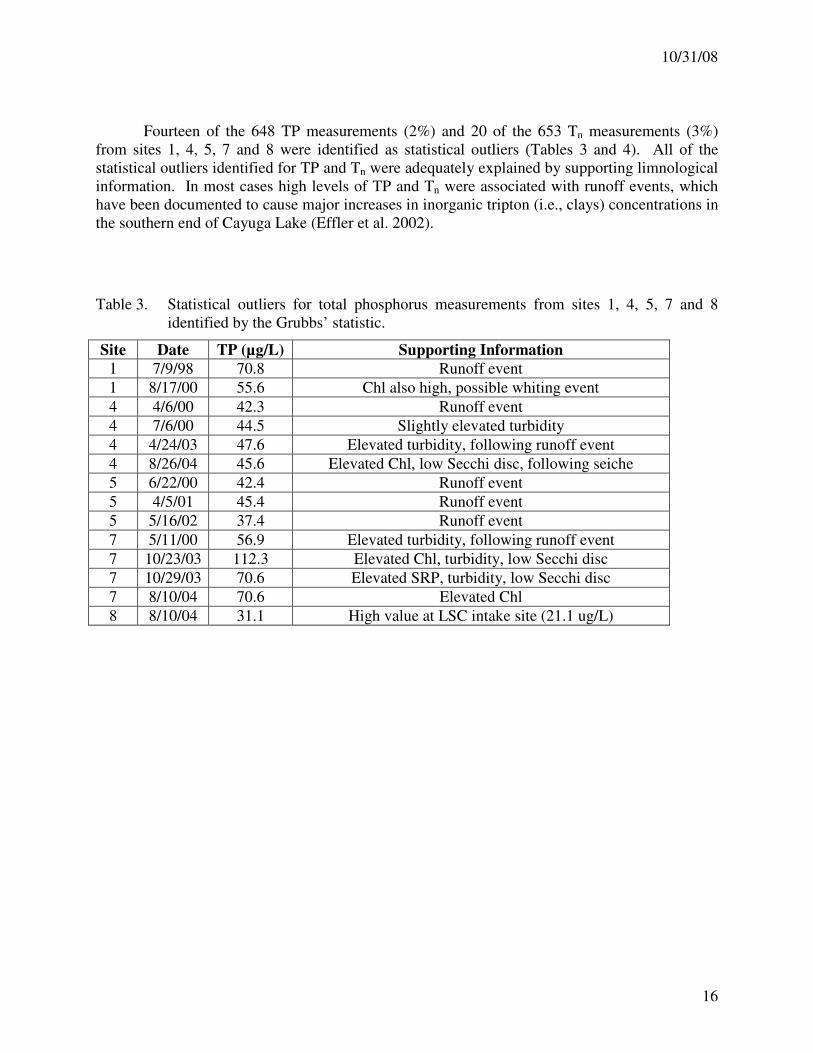
Fourteen of the 648 TP measurements (2%) and 20 of the 653 Tn measurements (3%)
from sites 1, 4, 5, 7 and 8 were identified as statistical outliers (Tables 3 and 4). All of the
statistical outliers identified for TP and Tn were adequately explained by supporting limnological
information. In most cases high levels of TP and Tn were associated with runoff events, which
have been documented to cause major increases in inorganic tripton (i.e., clays) concentrations in
the southern end of Cayuga Lake (Effler et al. 2002).
Table 3. Statistical outliers for total phosphorus measurements from sites 1, 4, 5, 7 and 8
identified by the Grubbs’ statistic.
Site Date TP (µg/L) Supporting Information
1 7/9/98 70.8 Runoff event
1 8/17/00 55.6 Chl also high, possible whiting event
4 4/6/00 42.3 Runoff event
4 7/6/00 44.5 Slightly elevated turbidity
4 4/24/03 47.6 Elevated turbidity, following runoff event
4 8/26/04 45.6 Elevated Chl, low Secchi disc, following seiche
5 6/22/00 42.4 Runoff event
5 4/5/01 45.4 Runoff event
5 5/16/02 37.4 Runoff event
7 5/11/00 56.9 Elevated turbidity, following runoff event
7 10/23/03 112.3 Elevated Chl, turbidity, low Secchi disc
7 10/29/03 70.6 Elevated SRP, turbidity, low Secchi disc
7 8/10/04 70.6 Elevated Chl
8 8/10/04 31.1 High value at LSC intake site (21.1 ug/L)
10/31/08
17
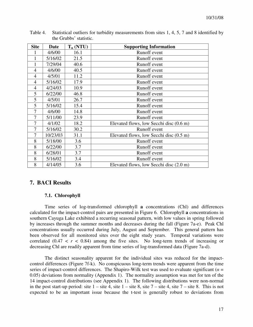
Table 4. Statistical outliers for turbidity measurements from sites 1, 4, 5, 7 and 8 identified by
the Grubbs’ statistic.
Site Date Tn (NTU) Supporting Information
1 4/6/00 16.1 Runoff event
1 5/16/02 21.5 Runoff event
1 7/29/04 40.6 Runoff event
4 4/6/00 40.5 Runoff event
4 4/5/01 11.2 Runoff event
4 5/16/02 17.9 Runoff event
4 4/24/03 10.9 Runoff event
5 6/22/00 46.8 Runoff event
5 4/5/01 26.7 Runoff event
5 5/16/02 15.4 Runoff event
7 4/6/00 14.8 Runoff event
7 5/11/00 23.9 Runoff event
7 4/1/02 18.2 Elevated flows, low Secchi disc (0.6 m)
7 5/16/02 30.2 Runoff event
7 10/23/03 31.1 Elevated flows, low Secchi disc (0.5 m)
8 5/18/00 3.6 Runoff event
8 6/22/00 3.7 Runoff event
8 6/28/01 3.7 Runoff event
8 5/16/02 3.4 Runoff event
8 4/14/05 3.6 Elevated flows, low Secchi disc (2.0 m)
7. BACI Results
7.1. Chlorophyll
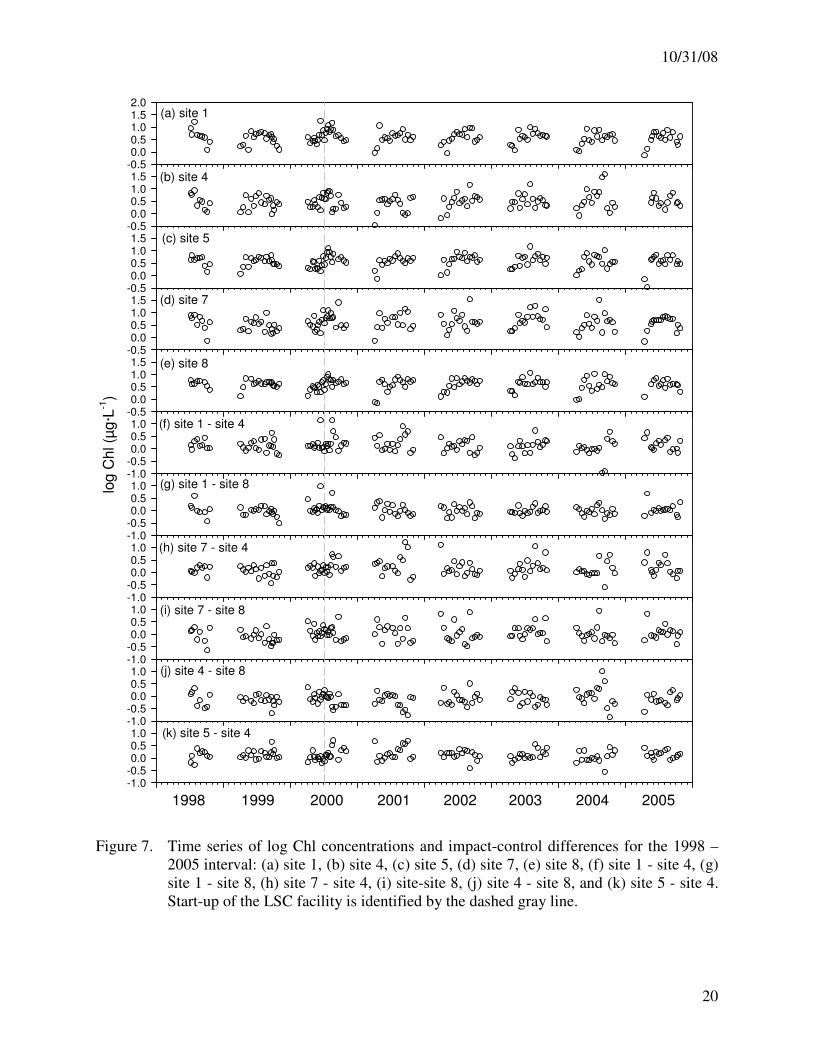
Time series of log-transformed chlorophyll a concentrations (Chl) and differences
calculated for the impact-control pairs are presented in Figure 6. Chlorophyll a concentrations in
southern Cayuga Lake exhibited a recurring seasonal pattern, with low values in spring followed
by increases through the summer months and decreases during the fall (Figure 7a-e). Peak Chl
concentrations usually occurred during July, August and September. This general pattern has
been observed for all monitored sites over the eight study years. Temporal variations were
correlated (0.47 < r < 0.84) among the five sites. No long-term trends of increasing or
decreasing Chl are readily apparent from time series of log-transformed data (Figure 7a-d).
The distinct seasonality apparent for the individual sites was reduced for the impact-
control differences (Figure 7f-k). No conspicuous long-term trends were apparent from the time
series of impact-control differences. The Shapiro-Wilk test was used to evaluate significant (α =
0.05) deviations from normality (Appendix 1). The normality assumption was met for ten of the
14 impact-control distributions (see Appendix 1). The following distributions were non-normal
in the post start-up period: site 1 – site 4, site 1 – site 8, site 7 – site 4, site 7 – site 8. This is not
expected to be an important issue because the t-test is generally robust to deviations from
10/31/08
18
normality and sample sizes are large enough to invoke the Central Limit Theorem. Differences
calculated from the site 7 – site 4 pairing showed significant negative serial correlation in the
pre-LSC period (lag 1 r = -0.32) and positive correlation during the post-LSC period (lag 1 r =
0.25) (Appendix 2). Positive serial correlation was observed for the following impact-control
pairings during the post start-up period: site1 – site 4 (lag 1 r = 0.30), site 4 – site 8 (lag 1 r =
0.25), site 5 – site 4 (lag 1 r = 0.20). Serial correlation was low (r < 0.2) for the other impact-
control pairs. No serious violations of the additivity assumption were detected based on the
weak (r2 ≤ 0.2) relationships observed between the differences and averages for log Chl
(Appendix 3).
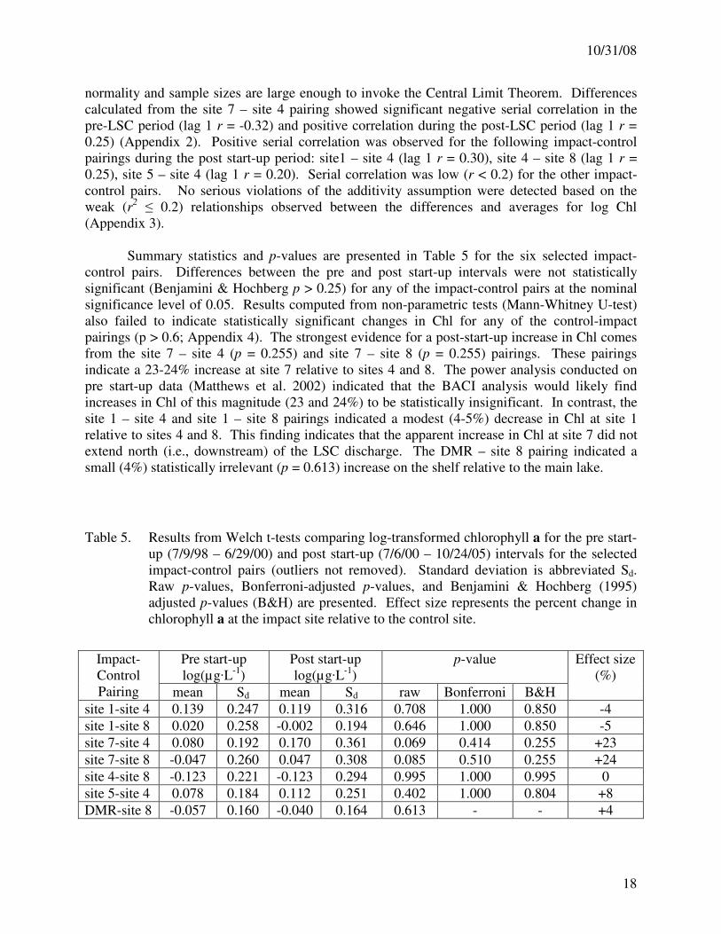
Summary statistics and p-values are presented in Table 5 for the six selected impact-
control pairs. Differences between the pre and post start-up intervals were not statistically
significant (Benjamini & Hochberg p > 0.25) for any of the impact-control pairs at the nominal
significance level of 0.05. Results computed from non-parametric tests (Mann-Whitney U-test)
also failed to indicate statistically significant changes in Chl for any of the control-impact
pairings (p > 0.6; Appendix 4). The strongest evidence for a post-start-up increase in Chl comes
from the site 7 – site 4 (p = 0.255) and site 7 – site 8 (p = 0.255) pairings. These pairings
indicate a 23-24% increase at site 7 relative to sites 4 and 8. The power analysis conducted on
pre start-up data (Matthews et al. 2002) indicated that the BACI analysis would likely find
increases in Chl of this magnitude (23 and 24%) to be statistically insignificant. In contrast, the
site 1 – site 4 and site 1 – site 8 pairings indicated a modest (4-5%) decrease in Chl at site 1
relative to sites 4 and 8. This finding indicates that the apparent increase in Chl at site 7 did not
extend north (i.e., downstream) of the LSC discharge. The DMR – site 8 pairing indicated a
small (4%) statistically irrelevant (p = 0.613) increase on the shelf relative to the main lake.
Table 5. Results from Welch t-tests comparing log-transformed chlorophyll a for the pre start-
up (7/9/98 – 6/29/00) and post start-up (7/6/00 – 10/24/05) intervals for the selected
impact-control pairs (outliers not removed). Standard deviation is abbreviated Sd.
Raw p-values, Bonferroni-adjusted p-values, and Benjamini & Hochberg (1995)
adjusted p-values (B&H) are presented. Effect size represents the percent change in
chlorophyll a at the impact site relative to the control site.
Impact-
Control
Pairing
Pre start-up
log(µg·L-1
)
Post start-up
log(µg·L-1
)
p-value Effect size
(%)
mean Sd mean Sd raw Bonferroni B&H
site 1-site 4 0.139 0.247 0.119 0.316 0.708 1.000 0.850 -4
site 1-site 8 0.020 0.258 -0.002 0.194 0.646 1.000 0.850 -5
site 7-site 4 0.080 0.192 0.170 0.361 0.069 0.414 0.255 +23
site 7-site 8 -0.047 0.260 0.047 0.308 0.085 0.510 0.255 +24
site 4-site 8 -0.123 0.221 -0.123 0.294 0.995 1.000 0.995 0
site 5-site 4 0.078 0.184 0.112 0.251 0.402 1.000 0.804 +8
DMR-site 8 -0.057 0.160 -0.040 0.164 0.613 - - +4
10/31/08
19
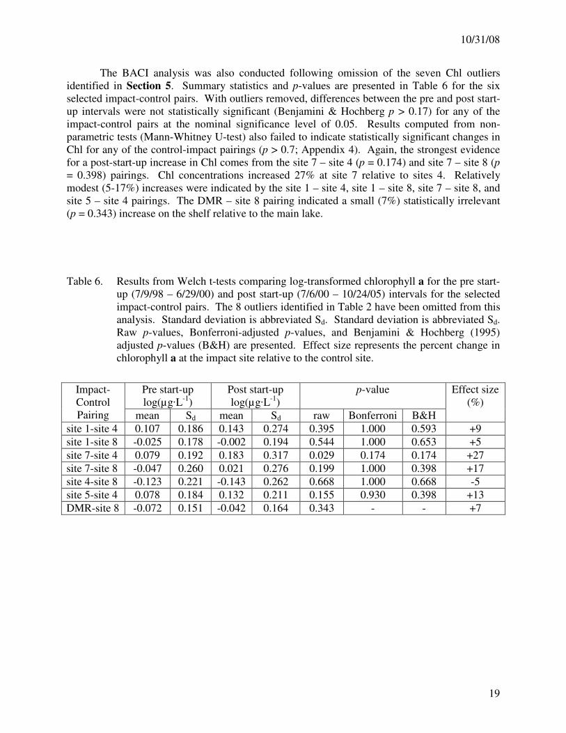
The BACI analysis was also conducted following omission of the seven Chl outliers
identified in Section 5. Summary statistics and p-values are presented in Table 6 for the six
selected impact-control pairs. With outliers removed, differences between the pre and post start-
up intervals were not statistically significant (Benjamini & Hochberg p > 0.17) for any of the
impact-control pairs at the nominal significance level of 0.05. Results computed from non-
parametric tests (Mann-Whitney U-test) also failed to indicate statistically significant changes in
Chl for any of the control-impact pairings (p > 0.7; Appendix 4). Again, the strongest evidence
for a post-start-up increase in Chl comes from the site 7 – site 4 (p = 0.174) and site 7 – site 8 (p
= 0.398) pairings. Chl concentrations increased 27% at site 7 relative to sites 4. Relatively
modest (5-17%) increases were indicated by the site 1 – site 4, site 1 – site 8, site 7 – site 8, and
site 5 – site 4 pairings. The DMR – site 8 pairing indicated a small (7%) statistically irrelevant
(p = 0.343) increase on the shelf relative to the main lake.
Table 6. Results from Welch t-tests comparing log-transformed chlorophyll a for the pre start-
up (7/9/98 – 6/29/00) and post start-up (7/6/00 – 10/24/05) intervals for the selected
impact-control pairs. The 8 outliers identified in Table 2 have been omitted from this
analysis. Standard deviation is abbreviated Sd. Standard deviation is abbreviated Sd.
Raw p-values, Bonferroni-adjusted p-values, and Benjamini & Hochberg (1995)
adjusted p-values (B&H) are presented. Effect size represents the percent change in
chlorophyll a at the impact site relative to the control site.
Impact-
Control
Pairing
Pre start-up
log(µg·L-1
)
Post start-up
log(µg·L-1
)
p-value Effect size
(%)
mean Sd mean Sd raw Bonferroni B&H
site 1-site 4 0.107 0.186 0.143 0.274 0.395 1.000 0.593 +9
site 1-site 8 -0.025 0.178 -0.002 0.194 0.544 1.000 0.653 +5
site 7-site 4 0.079 0.192 0.183 0.317 0.029 0.174 0.174 +27
site 7-site 8 -0.047 0.260 0.021 0.276 0.199 1.000 0.398 +17
site 4-site 8 -0.123 0.221 -0.143 0.262 0.668 1.000 0.668 -5
site 5-site 4 0.078 0.184 0.132 0.211 0.155 0.930 0.398 +13
DMR-site 8 -0.072 0.151 -0.042 0.164 0.343 - - +7
10/31/08
20
-0.50.00.51.01.52.0
(a) site 1
-0.50.00.51.01.5 (b) site 4
-0.50.00.51.01.5 (c) site 5
-0.50.00.51.01.5
log C
hl (µ
g·L
-1)
-1.0-0.50.00.51.0
-1.0-0.50.00.51.0
(e) site 8
(f) site 1 - site 4
(g) site 1 - site 8
-1.0-0.50.00.51.0 (j) site 4 - site 8
-1.0-0.50.00.51.0 (k) site 5 - site 4
1998 1999 2000 2001 2002 2003
-0.50.00.51.01.5 (d) site 7
-1.0-0.50.00.51.0 (h) site 7 - site 4
-1.0-0.50.00.51.0 (i) site 7 - site 8
2004 2005
Figure 7. Time series of log Chl concentrations and impact-control differences for the 1998 –
2005 interval: (a) site 1, (b) site 4, (c) site 5, (d) site 7, (e) site 8, (f) site 1 - site 4, (g)
site 1 - site 8, (h) site 7 - site 4, (i) site-site 8, (j) site 4 - site 8, and (k) site 5 - site 4.
Start-up of the LSC facility is identified by the dashed gray line.
10/31/08
21
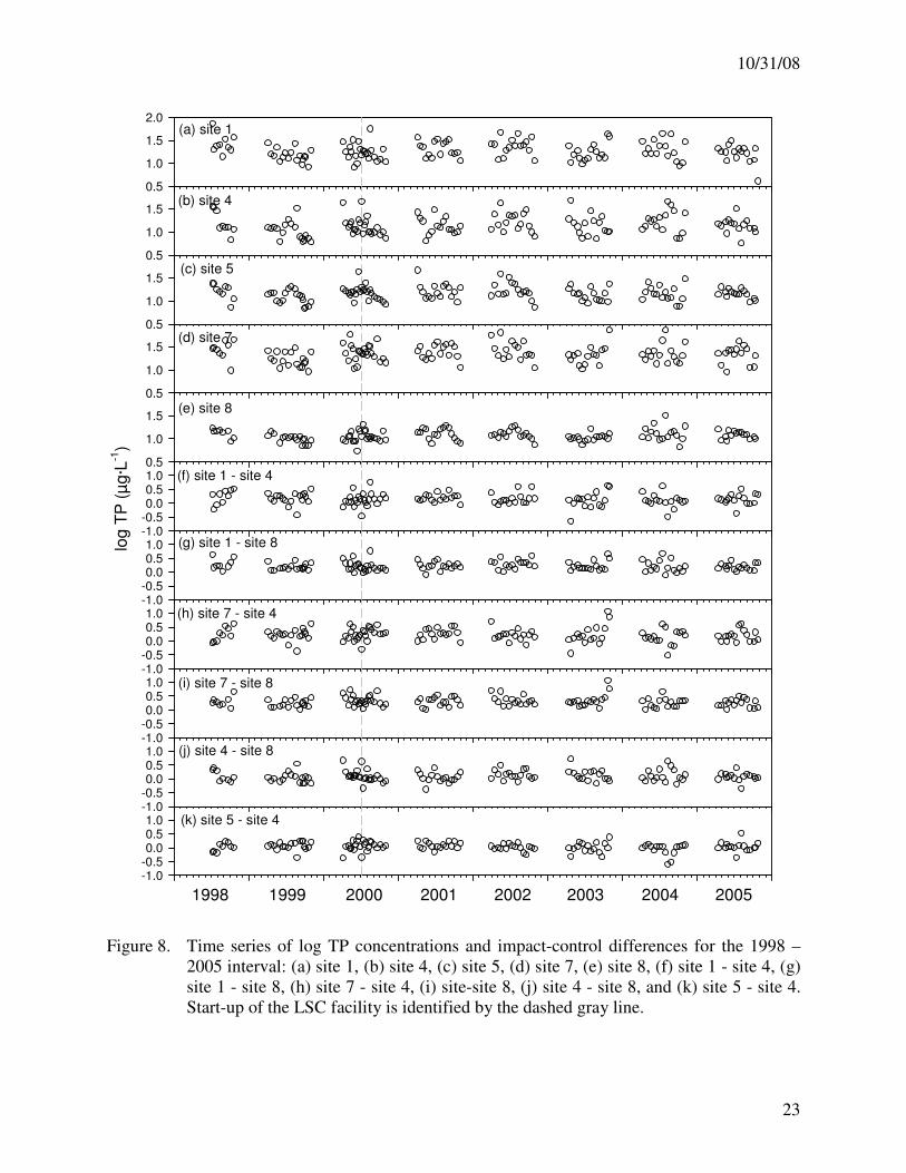
7.2. Total Phosphorus
Time series of log-transformed total phosphorus concentrations (TP) and differences
calculated for the impact-control pairs are presented in Figure 8. In contrast to Chl, TP did not
exhibit a recurring seasonal pattern in southern Cayuga Lake (Figure 8a-e). The highest TP
concentrations on the shelf have generally been observed during periods of high runoff (UFI
1999, 2000, 2001, 2002, 2003, 2004, 2005, 2006) when terrigenous inputs of inorganic tripton
are greatest. Effler et al. (2002) found that ~ 50% of the TP on the shelf over the June – October
interval of 1999 was tripton. The time period included in this study was particularly dry and it is
likely that contributions from tripton to the TP pool are even higher during high flow intervals
(Effler et. al. 2002). Total phosphorus concentrations have been relatively high during spring
(Figure 8a-e), indicative of contributions from terrigenous inputs. Summertime peaks in TP
(Figure 8a-e) that coincided with peaks in Chl (Figure 7a-e) were observed at various sites over
the eight-year study period. However, correlations between paired measurements of log TP and
log Chl for the five sites were weak (r < 0.4). Temporal variations in log TP were correlated
(0.32 < r < 0.68) among the four sites. The strongest correlation (r = 0.68) was between sites 1
and 7 and the weakest (0.32) between sites 7 and 4. No long-term trends of increasing or
decreasing TP are readily apparent from time series of log-transformed data (Figure 8a-e).
No distinct seasonality or conspicuous long-term trends were apparent for the impact-
control differences (Figure 8f-k). The Shapiro-Wilk test was used to evaluate significant (α =
0.05) deviations from normality (Appendix 1). The normality assumption was met for six of the
14 impact-control distributions (see Appendix 1). Three distributions were non-normal in the pre
start-up period (site 1 – site 8, site 4 – site 8, DMR – site 8) and five distributions were non-
normal in the post start-up period (site 1 – site 4, site 1 – site 8, site 7 – site 8, site 4 – site 8, site
5 – site 4). Although eight of the 14 impact-control distributions violated the normality
assumption (Appendix 1), this is not expected to invalidate the results of t-tests. The t-test is
generally robust to deviations from normality and sample sizes are large enough to invoke the
Central Limit Theorem. Significant positive serial correlation was evident for the DMR – site 8
pairing during the pre-LSC interval (lag 1 r = 0.30). Differences calculated from the site 7 – site
4 (lag 1 r = 0.21) and site 5 – site 4 (lag 1 r = 0.23) pairings showed significant positive serial
correlation in the post-LSC period (Appendix 2). Serial correlation was low (r < 0.2) for the
other impact-control pairs. The additivity assumption was violated for pairings with site 8 as the
control site (Appendix 3). This is a result of the disproportionate impact of runoff events on TP
concentrations on the shelf compared to site 8.
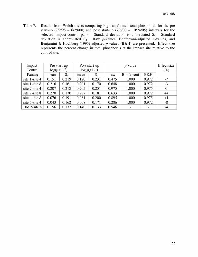
Summary statistics and p-values are presented in Table 7 for the six selected impact-
control pairs. Differences between the pre and post start-up intervals were not statistically
significant (Benjamini & Hochberg p > 0.97) for any of the impact-control pairs at the nominal
significance level of 0.05. Results computed from non-parametric tests (Mann-Whitney U-test)
also failed to indicate statistically significant changes in TP for any of the control-impact
pairings (p > 0.9; Appendix 4). Effect sizes were small (<10%) and there was no evidence for
substantial changes in TP following start-up of the LSC facility. The DMR – site 8 pairing
indicated a small (4%) statistically irrelevant (p = 0.546) decrease on the shelf relative to the
main lake.
10/31/08
22
Table 7. Results from Welch t-tests comparing log-transformed total phosphorus for the pre
start-up (7/9/98 – 6/29/00) and post start-up (7/6/00 – 10/24/05) intervals for the
selected impact-control pairs. Standard deviation is abbreviated Sd. Standard
deviation is abbreviated Sd. Raw p-values, Bonferroni-adjusted p-values, and
Benjamini & Hochberg (1995) adjusted p-values (B&H) are presented. Effect size
represents the percent change in total phosphorus at the impact site relative to the
control site.
Impact-
Control
Pairing
Pre start-up
log(µg·L-1
)
Post start-up
log(µg·L-1
)
p-value Effect size
(%)
mean Sd mean Sd raw Bonferroni B&H
site 1-site 4 0.151 0.219 0.120 0.231 0.475 1.000 0.972 -7
site 1-site 8 0.216 0.161 0.201 0.170 0.648 1.000 0.972 -3
site 7-site 4 0.207 0.218 0.205 0.251 0.975 1.000 0.975 0
site 7-site 8 0.270 0.170 0.287 0.181 0.633 1.000 0.972 +4
site 4-site 8 0.076 0.191 0.081 0.200 0.895 1.000 0.975 +1
site 5-site 4 0.043 0.162 0.008 0.171 0.286 1.000 0.972 -8
DMR-site 8 0.156 0.132 0.140 0.133 0.546 - - -4
10/31/08
23
0.5
1.0
1.5
2.0(a) site 1
0.5
1.0
1.5(b) site 4
0.5
1.0
1.5(c) site 5
0.5
1.0
1.5
log T
P (
µg·L
-1)
-1.0-0.50.00.51.0
-1.0-0.50.00.51.0
(e) site 8
(f) site 1 - site 4
(g) site 1 - site 8
-1.0-0.50.00.51.0 (j) site 4 - site 8
-1.0-0.50.00.51.0 (k) site 5 - site 4
1998 1999 2000 2001 2002 2003
0.5
1.0
1.5(d) site 7
-1.0-0.50.00.51.0 (h) site 7 - site 4
-1.0-0.50.00.51.0 (i) site 7 - site 8
2004 2005
Figure 8. Time series of log TP concentrations and impact-control differences for the 1998 –
2005 interval: (a) site 1, (b) site 4, (c) site 5, (d) site 7, (e) site 8, (f) site 1 - site 4, (g)
site 1 - site 8, (h) site 7 - site 4, (i) site-site 8, (j) site 4 - site 8, and (k) site 5 - site 4.
Start-up of the LSC facility is identified by the dashed gray line.
10/31/08
24
7.3. Turbidity
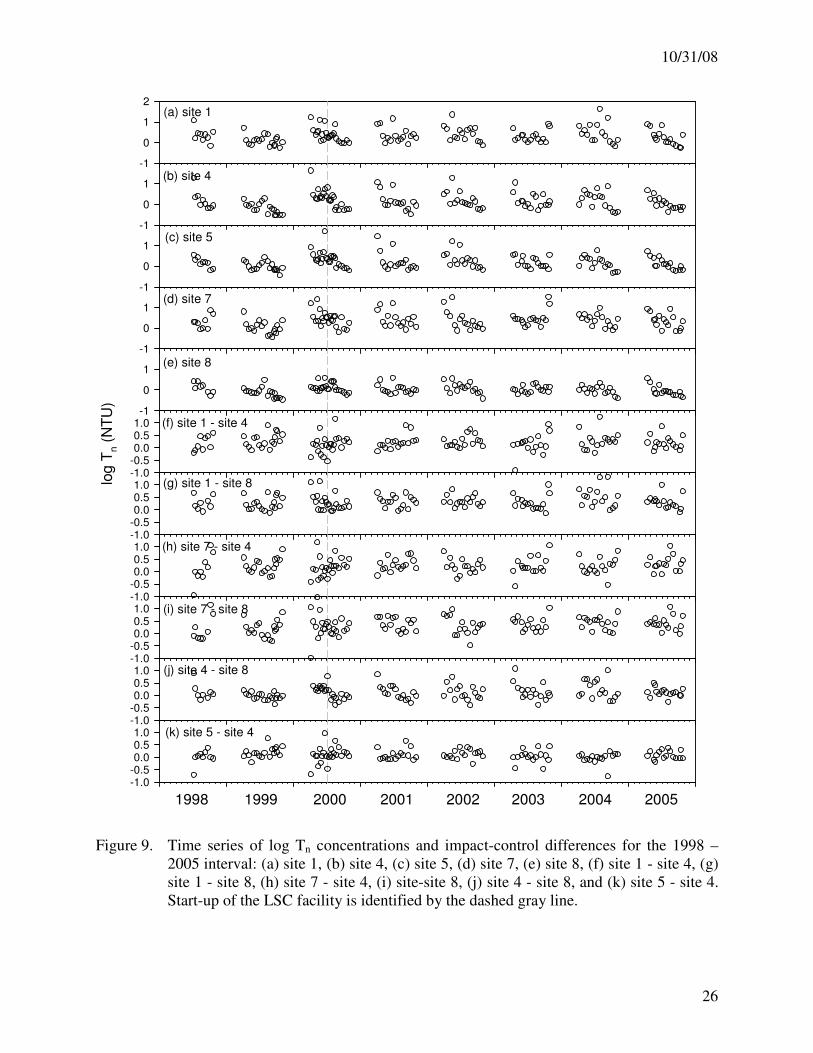
Time series of log-transformed turbidity values (Tn) and differences calculated for the
impact-control pairs are presented in Figure 9. Turbidity values have varied widely, both among
sites and over time at individual sites (Figure 9a-e). Effler et al. (2002) found that inorganic
tripton, rather than phytoplankton biomass, is the primary regulator of Tn (clarity) in southern
Cayuga Lake, and that the higher levels of these constituents (particularly clay minerals) on the
shelf are responsible for the generally higher Tn (lower clarity) values observed in this portion of
the lake. Elevated turbidity on the shelf is not surprising considering its location with respect to
major tributaries and the susceptibility of this shallow area to wind driven resuspension (Figure
1). The extremely high Tn values that accompany major runoff events (Figure 9a-e; see also UFI
1999, 2000, 2001, 2002, 2003, 2005, 2005, 2006) serve to inflate temporal variability and cause
mean values to be highly uncertain. Compared to the shelf sites, the deep water sampling
location (sites 8) exhibits much lower variability and, in general, substantially lower Tn values
(Figure 9e). Paired measurements of log Tn and log TP were positively correlated for all five
sites (r > 0.43). The coupling between these two variables was particularly strong (r > 0.6) for
the shelf sites. Temporal variations in log Tn were positively correlated (0.44 < r < 0.79) among
the four shelf sites. No long-term trends of increasing or decreasing Tn levels are readily
apparent from these time series (Figure 9a-e).
No obvious long-term trends were apparent from the time series of impact-control
differences (Figure 9f-k). The normality assumption was not met for twelve of the 14 impact-
control pairs (Appendix 1). For the reasons stated above, this is not considered a serious issue
for the t-tests conducted as part of the BACI analysis. Impact-control differences for log Tn were
significantly serially correlated for the following impact-control pairs in the post start-up period:
site 7 – site 4, site 7 – site 8, site 4 – site 8 (Appendix 2). The additivity assumption was violated
for pairings with site 8 as the control site (Appendix 3). As with TP, this is a result of the
disproportionate impact of runoff events on the shelf compared to site 8.
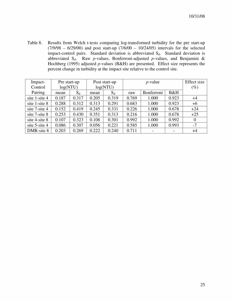
Summary statistics and p-values are presented in Table 8 for the six selected impact-
control pairs. Differences between the pre and post start-up intervals were not statistically
significant (Benjamini & Hochberg p > 0.67) for any of the impact-control pairs at the nominal
significance level of 0.05. Results computed from non-parametric tests (Mann-Whitney U-test)
also failed to indicate statistically significant changes in Tn for any of the control-impact pairings
(p > 0.2; Appendix 4). The strongest evidence for a post-start-up increase in Tn comes from the
site 7 – site 4 (p = 0.678) and site 7 – site 8 (p = 0.678) pairings. These pairings indicate a 24-
25% increase at site 7 relative to sites 4 and 8. Modest increases in Tn were indicated for site 1
relative to control sites, which suggests that the apparent increase in Tn at site 7 did not extend
north (i.e., downstream) of the LSC discharge. The DMR – site 8 pairing indicated a small (4%)
statistically irrelevant (p = 0.711) increase on the shelf relative to the main lake.
10/31/08
25
Table 8. Results from Welch t-tests comparing log-transformed turbidity for the pre start-up
(7/9/98 – 6/29/00) and post start-up (7/6/00 – 10/24/05) intervals for the selected
impact-control pairs. Standard deviation is abbreviated Sd. Standard deviation is
abbreviated Sd. Raw p-values, Bonferroni-adjusted p-values, and Benjamini &
Hochberg (1995) adjusted p-values (B&H) are presented. Effect size represents the
percent change in turbidity at the impact site relative to the control site.
Impact-
Control
Pairing
Pre start-up
log(NTU)
Post start-up
log(NTU)
p-value Effect size
(%)
mean Sd mean Sd raw Bonferroni B&H
site 1-site 4 0.187 0.317 0.205 0.319 0.769 1.000 0.923 +4
site 1-site 8 0.288 0.312 0.313 0.291 0.683 1.000 0.923 +6
site 7-site 4 0.152 0.419 0.245 0.331 0.226 1.000 0.678 +24
site 7-site 8 0.253 0.430 0.351 0.313 0.216 1.000 0.678 +25
site 4-site 8 0.107 0.323 0.108 0.301 0.992 1.000 0.992 0
site 5-site 4 0.086 0.307 0.056 0.221 0.585 1.000 0.993 -7
DMR-site 8 0.203 0.269 0.222 0.240 0.711 - - +4
10/31/08
26
-1
0
1
2(a) site 1
-1
0
1(b) site 4
-1
0
1(c) site 5
-1
0
1
log T
n (
NT
U)
-1.0-0.50.00.51.0
-1.0-0.50.00.51.0
(e) site 8
(f) site 1 - site 4
(g) site 1 - site 8
-1.0-0.50.00.51.0 (j) site 4 - site 8
-1.0-0.50.00.51.0 (k) site 5 - site 4
1998 1999 2000 2001 2002 2003
-1
0
1(d) site 7
-1.0-0.50.00.51.0 (h) site 7 - site 4
-1.0-0.50.00.51.0 (i) site 7 - site 8
2004 2005
Figure 9. Time series of log Tn concentrations and impact-control differences for the 1998 –
2005 interval: (a) site 1, (b) site 4, (c) site 5, (d) site 7, (e) site 8, (f) site 1 - site 4, (g)
site 1 - site 8, (h) site 7 - site 4, (i) site-site 8, (j) site 4 - site 8, and (k) site 5 - site 4.
Start-up of the LSC facility is identified by the dashed gray line.
10/31/08
27
8. Limnological Interpretation
8.1. Introduction
The primary objective of this report was to determine if statistically significant changes
occurred in three water quality parameters (chlorophyll a, total phosphorus, turbidity) in the
southern portion of Cayuga Lake coincident in time with start-up of Cornell’s Lake Source
Cooling (LSC) facility. Quantitative decision criteria, determined by appropriate statistical
models and techniques are widely desired. However, the effective design, analysis, and
interpretation of environmental monitoring studies are formidable tasks fraught with difficult
statistical and limnological judgments. Examples of difficult judgments encountered in the
BACI analysis presented here include the selection of appropriate control-impact comparisons
and the choice of a suitable balance between the costs of Type I and Type II errors. Furthermore,
statistical impact analysis cannot, by itself, establish definitively the cause of a documented
change in water quality. Discovering the cause of any observed water quality changes in the
southern end of Cayuga Lake is particularly complicated because of the potential for
simultaneous changes in multiple drivers not associated with LSC operation. Natural variation in
meteorological conditions, improvements in treatment at domestic wastewater treatment plants,
and the uncertain effects of zebra mussel populations are potential confounding variables.
The issues encountered here are characteristic of observational studies and are not unique
to the BACI analysis for the LSC facility. Researchers have advocated a variety of alternate
methods for interpreting data from such studies, including the use of graphical presentation, the
informal use of statistical tests, expert judgment, and common sense (Stewart-Oaten 1995,
Murtaugh 2002). Ultimately, responsible assessment of potential water quality impacts
associated with LSC operation requires the integration of limnological and statistical analyses.
The purpose of this section is to focus on limnological interpretations rather than p-values
derived from hypothesis tests of questionable validity. The following issues are considered: the
relative contributions of LSC, wastewater treatment plants, and tributaries to material loading to
southern Cayuga Lake; the systematic increase in soluble reactive phosphorus concentrations
(SRP) in the hypolimnion of Cayuga Lake; hydraulic loading and residence time in the southern
shelf of Cayuga Lake; biological significance of observed water quality changes; and potential
effects of zebra mussel populations.
8.2. Material Loading Contributions to the Southern Shelf of Cayuga Lake
The potential for operation of the LSC facility to effect water quality conditions in the
southern shelf of Cayuga Lake is regulated to a large extent by material loading contributions.
The primary constituent of concern is TP, as Chl and Tn levels were routinely much lower in the
hypolimnion of Cayuga Lake (i.e., LSC effluent) than in the receiving waters of the southern
shelf (UFI 1999-2006). Although TP concentrations in the LSC effluent have been routinely
lower than those of the southern shelf, soluble reactive phosphorus concentrations (SRP) have
been a factor of 2 to 5 higher in the LSC discharge. SRP is a component of total dissolved
phosphorus (TDP) that is usually assumed to be immediately available to support phytoplankton
growth. Thus, the LSC discharge has the potential to increase phytoplankton biomass (i.e., Chl)
on the southern shelf. This potential impact was acknowledged in the Environmental Impact
Statement (Stearns and Wheler 1997) prepared for the LSC facility, which stated “The estimated
10/31/08
28
potential cumulative increase in concentration of chlorophyll a is approximately 2.5 µg/L (range
1.25 to 5 µg/L) over the June to October period. Even if the potential increase in phytoplankton
biomass is restricted to the region of the outfall, the increase in chlorophyll a would be very
small.”
The potential for phosphorus loading from LSC to affect phytoplankton biomass is small
relative to phosphorus inputs from wastewater treatment plants and tributaries. Following
upgrades in treatment at the Ithaca Area and Cayuga Heights WWTPs and under the low flow
conditions of 2007, LSC represented about 7.5% of the phosphorus loading to the southern shelf.
The maximum contribution of LSC to phosphorus loading on a monthly basis was 13% during
August of 2006 and 2007 (Cornell University 2008). The tributaries have been the dominant
source of phosphorus and turbidity to shelf, particularly during high runoff years (Effler et al.
2002, 2008). Despite the phosphorus loading received from local sources, summer average Chl
concentrations have not been substantially higher on the shelf compared to bounding pelagic
waters because of the high flushing rate of the shelf promoted by mixing with pelagic waters
(UFI 2008).
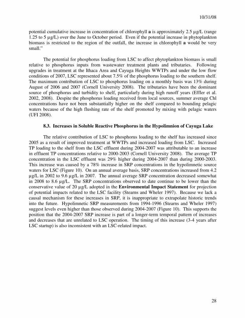
8.3. Increases in Soluble Reactive Phosphorus in the Hypolimnion of Cayuga Lake
The relative contribution of LSC to phosphorus loading to the shelf has increased since
2005 as a result of improved treatment at WWTPs and increased loading from LSC. Increased
TP loading to the shelf from the LSC effluent during 2004-2007 was attributable to an increase
in effluent TP concentrations relative to 2000-2003 (Cornell University 2008). The average TP
concentration in the LSC effluent was 29% higher during 2004-2007 than during 2000-2003.
This increase was caused by a 78% increase in SRP concentrations in the hypolimnetic source
waters for LSC (Figure 10). On an annual average basis, SRP concentrations increased from 4.2
µg/L in 2002 to 9.6 µg/L in 2007. The annual average SRP concentration decreased somewhat
in 2008 to 8.6 µg/L. The SRP concentrations observed to date continue to be lower than the
conservative value of 20 µg/L adopted in the Environmental Impact Statement for projection
of potential impacts related to the LSC facility (Stearns and Wheler 1997). Because we lack a
causal mechanism for these increases in SRP, it is inappropriate to extrapolate historic trends
into the future. Hypolimnetic SRP measurements from 1994-1996 (Stearns and Wheler 1997)
suggest levels even higher than those observed during 2004-2007 (Figure 10). This supports the
position that the 2004-2007 SRP increase is part of a longer-term temporal pattern of increases
and decreases that are unrelated to LSC operation. The timing of this increase (3-4 years after
LSC startup) is also inconsistent with an LSC-related impact.
10/31/08
29
SR
P (
µg·L
-1)
0
5
10
15
20
25
2000 2001 2002 2003 2004 2005 200820072006
assumed in EIS
Figure 10. Time series of SRP concentrations measured weekly in the LSC effluent for the 2000
– 2008 interval. LSC effluent concentrations are representative of the hypolimnetic
source water (UFI 2007). The dashed line represents the SRP concentration of 20
µg/L used in the Environmental Impact Statement to assess potential impacts of
the LSC facility (Stearns and Wheler 1997).
An unambiguous explanation for the apparent increases in TP, SRP, and Tn in the lake’s
hypolimnion has not been identified. In large deep lakes such as Cayuga, changes in
hypolimnetic water quality are expected to occur over long time scales, on the order of decades
rather than years. Temporary increases in Tn and the particulate fraction of TP in bottom waters
can be caused by plunging turbid inflows and internal waves or seiches. However, hypolimnetic
SRP levels are generally considered to reflect lake-wide metabolism rather than local effects.
Soluble reactive phosphorus is produced during microbial decomposition of organic matter and
often accumulates in the hypolimnia of stratifying lakes during summer. Increases in primary
production (phytoplankton growth) and subsequent decomposition could cause increases in SRP
levels, but noteworthy increases in chlorophyll concentrations (phytoplankton biomass) have not
been observed. Longer intervals of thermal stratification, increased hypolimnetic temperatures
or depletion of dissolved oxygen could also cause higher concentrations of SRP in the bottom
waters. Such changes have not been observed. The apparent increase in hypolimnetic SRP
concentrations may represent a short-term anomaly rather than a long-term trend. Regardless,
this phenomenon has the potential to affect phosphorus loading to the shelf from the LSC
effluent and should be diligently monitored in the future in order to discern the permanence and
significance of these changes.
8.4. Hydraulic Loading and Residence Time in the Southern Shelf of Cayuga Lake
Substantial interannual variations in hydrologic loading to the southern shelf occurred
over the 1998-2007 interval, driven primarily by natural variations in runoff from tributaries
(UFI 2008). These variations in runoff have caused conspicuous water quality signatures in the
shelf, as manifested in higher levels of TP, Tn, and Chl in high runoff years (Cornell University
2008). It is noteworthy that 1999, the only complete year of pre start-up data, was the lowest
runoff year of the 1998 – 2005 interval. Runoff was also relatively low in 2001 and 2005, and
relatively high in 2000, 2002, 2003, and 2004. The average inflow rate to the shelf for the April-
October interval increased approximately 11% following start-up of the LSC facility in 2000
(UFI 2008). However, the LSC effluent contributes more than 50% of the inflow to the shelf
during low runoff summertime periods (UFI 2003). UFI (2008) reported that the shelf is flushed
10/31/08
30
rapidly, approximately once per day during the May – October interval. The high flushing rate
of the shelf is caused primarily by exchange with water from the main lake. Wind-induced
upwelling events occur commonly on the shelf and promote exchange with metalimnetic and
hypolimnetic waters of the pelagic zone. The rapid exchange of shelf waters with those of the
main lake discourages the development of gradients in Chl from local phosphorus loading to the
shelf.
Preliminary numerical simulations conducted with an unvalidated three dimensional (3-
D) free surface hydrodynamic model suggest that the exchange of water in and out of the shelf is
affected by both inflow events and the internal wave oscillations (personal communication with
E. Cowen, Cornell University). Preliminary model results also indicate that transport in-out of
the shelf is lower in magnitude during non-inflow events at site 7 than at sites 1 and 4. The
relative isolation of site 7 from the pelagic waters may contribute to the higher levels of Chl, TP,
and Tn at this location. However, water quality conditions at site 7 are also likely to be
influenced by the proximity of this site to WWTP discharges. The effects of the LSC effluent on
flow patterns in the shelf have not been documented, although it has undoubtedly increased
flushing rates on the shelf during low runoff periods.
8.5. Biological Significance of Observed Water Quality Changes
The strongest evidence for water quality changes following LSC start-up was a 27%
increase in Chl at site 7 relative to site 4 (Table 6) and a 24% increase in Tn at site 7 relative to
site 8 (Table 8). Although the magnitude of these effects was found to be statistically
insignificant, it is important to evaluate the potential biological significance of these changes.
Admittedly, the assessment of biological significance is no less complex or subjective than the
assessment of statistical significance. The 27% increase in Chl at site 7 relative to site 4 is
equivalent to an additional increase of approximately 1 µg/L at site 7. An increase of this
magnitude would likely be deemed noteworthy in the pelagic waters of an oligotrophic lake, but
probably not in the littoral zone of a heavily impacted mesotrophic lake. The 27% increase in Tn
at site 7 relative to site 8 is equivalent to an additional increase of approximately 1 NTU at site 7.
Again, an increase of this magnitude might be considered noteworthy in the pelagic waters of an
oligotrophic lake, but it would probably not be a major cause for concern in the
anthropogenically perturbed littoral zone of a mesotrophic lake. In other words, variations of a
similar magnitude are not uncommon in lakes.
The apparent large scale increase in Chl depicted in Figure 2 is perhaps more noteworthy,
and an obvious cause for this change is not apparent. However, it is important to note that higher
Chl concentrations were measured on the shelf during 1994 – 1996. Chl concentrations on the
shelf decreased 35% from 1994 – 1996 to 1998 – 1999 in the absence of any documented
perturbation. The recent increase in Chl on the shelf has resulted in a rebound to levels observed
during 1994-1996. The large spatial extent of this change is not consistent with the type of
localized impact that might be expected as a result of LSC operation. It is likely that the
association between LSC start-up and this increase in Chl is coincidental rather than causal.
10/31/08
31
8.6. Potential Effects of Zebra Mussel Populations
Dense populations of zebra mussels have been demonstrated to cause major changes in
common measures of water quality associated with various aspects of their metabolism. In
particular, conspicuous reductions in Chl and increases in clarity have been documented for a
number of aquatic ecosystems in North America associated with the filter feeding of this exotic
invader (e.g., Effler et al. 1996, Caraco et al. 1997). Effects on phosphorus cycling are less
straightforward; e.g., decreases in the particulate fraction may result from filter feeding while
excretion causes increases in the dissolved fraction (Arnott and Vanni 1996, Effler et al. 1997).
Hecky et al. (2003) developed a conceptual model called the nearshore shunt that describes the
redirection of nutrient and energy flow caused by dense zebra mussel populations. The
nearshore shunt has been linked to degraded water quality in nearshore zones in many parts of
the Laurentian Great Lakes, including the proliferation of the benthic filamentous alga
Cladophora. Improved water clarity associated with the filter feeding of zebra mussels resulted
in increased macrophyte habitat, species richness, frequency of occurrence, and community
composition in nearby Oneida Lake (Zhu et al. 2006). Dense macrophyte beds can be a nuisance
to boaters and are often considered a symptom of degraded water quality. Shifts in the density of
Cayuga Lake’s zebra mussel population could cause larger changes in trophic state indicators
than any associated with management actions to reduce inputs of phosphorus.
9. Summary
A Before-After-Control-Impact (BACI) design was applied to in-lake monitoring data
collected over the 1998 – 2005 interval for three water quality parameters (chlorophyll a, total
phosphorus, turbidity) to determine whether statistically significant changes occurred in the
southern portion of Cayuga Lake coincident in time with start-up of Cornell’s Lake Source
Cooling (LSC) facility. The BACI analysis included data from six in-lake sites, and seven
impact-control pairings were considered. Statistical significance was assessed using p-values
adjusted for multiple comparisons according to the method of Benjamini and Hochberg (1995),
which is the most powerful of the widely used methods to control Type I errors or the occurrence
of false positives. No statistically significant (α = 0.05) impacts were found for the three water
quality parameters on any of the seven impact-control pairs. Nonparametric test results (Mann-
Whitney U-test; Appendix 4) also failed to reveal statistically significant (α = 0.05) changes in
water quality.
The strongest evidence for a water quality impact coincident in time with LSC start-up
was indicated by increases of approximately 25% in chlorophyll a concentrations (Chl) and
turbidity levels (Tn) at site 7 relative to sites 4 and 8. The magnitude of these increases (~ 1
µg/L, ~ 1 NTU) was small and changes of this size are common in moderately productive lakes.
The apparent increase in Chl at site 7 was less than the potential cumulative increase of 1.25 to 5
µg/L estimated in the Environmental Impact Statement (Stearns and Wheler 1997). The
absence of similar increases in total phosphorus concentrations (TP) complicates interpretation
of these results because both phytoplankton and the particles that cause turbidity contain
phosphorus. Interpretations are further confounded by the absence of substantial increases in Chl
or Tn at site 1, perhaps the site most likely to be impacted by the LSC discharge. Preliminary
hydrodynamic modeling suggests transport in-out of the shelf is lower in magnitude during non-
inflow events at site 7 than at sites 1 and 4. The relative isolation of site 7 from the pelagic

10/31/08
32
waters may contribute to the higher levels of Chl, TP, and Tn at this location. The effects of the
LSC effluent on flow patterns in the shelf have not been documented, although it has
undoubtedly increased flushing rates on the shelf during low runoff periods. Average Chl
concentrations increased in the post LSC start-up period at eight of the nine sites monitored in
this study. Because of the relatively small contributions of the LSC discharge to TP loading on
the southern shelf (< 10%), it is unlikely that LSC was the direct cause of these increases.
10/31/08
33
References
APHA (American Public Health Association). 1992. Standard Methods for the Examination of
Water and Wastewater, 18th edition. American Public Health Assoc., Washington, DC.
APHA (American Public Health Association). 1996. Standard Methods for the Examination of
Water and Wastewater, 20th edition. American Public Health Assoc., Washington, DC.
Arnott, D. L. and M. J. Vanni. 1996. Nitrogen and phosphorus recycling by the zebra mussel
(Dreissena polymorpha) in the western basin of Lake Erie. Can. J. Fish. Aquat. Sci.
53:646-659.
Benjamini, Y. and Y. Hochberg. 1995. Controlling the false discovery rate: a practical and
powerful approach to multiple testing. J. R. Statist. Soc. B 57:289-300.
Caraco, N. F., J. J. Cole, P. A. Raymond, D. L. Strayer, M. L. Pace, S. E. G. Findlay and D. T.
Fischer. 1997. Zebra mussel invasion in a large, turbid river: Phytoplankton response to
increased grazing. Ecology 78:588-602.
Carlson, R. F. 1977. A trophic status index for lakes. Limnol. Oceanogr. 22:361-368.
Carpenter, S. R., T. M. Frost, D. Heisey and T. K. Kratz. 1989. Randomized intervention
analysis and the interpretation of whole-ecosystem experiments. Ecol. 70:1142-1152.
Cornell University. 2008. Cayuga Lake water quality monitoring related to the LSC Facility:
2007.
Eberhardt, L. L. and J. M. Thomas. 1991. Designing environmental field studies. Ecol. Monogr.
61:53-73.
Effler, S. W., M. T. Auer and N. A. Johnson. 1989. Modeling Cl concentration in Cayuga Lake,
USA. Water Air Soil Pollut. 44:347-362.
Effler, S. W., S. R. Boone, C. A. Siegfried, L. Walrath and S. L. Ashby. 1997. Mobilization of
ammonia and phosphorus by zebra mussels ( Dreissena polymorpha) in the Seneca River,
New York. P. 187-208. In F. M. D'Itri (ed). Zebra Mussels and Aquatic Nuisance
Species. Ann Arbor Press, Chelsea, Michigan.
Effler, S. W., C. M. Brooks, K. A. Whitehead, B. Wagner, S. M. Doerr, M. G. Perkins, C. A.
Siegfried, L. Walrath and R. P. Canale. 1996. Impact of zebra mussel invasion on river
water quality. Wat. Environ. Res. 68:205-214.
Effler, S. W., D. A. Matthews, M. G. Perkins, D. L. Johnson, F. Peng, M. R. Penn and M. T.
Auer. 2002. Patterns and impacts of inorganic tripton in Cayuga Lake. Hydrobiologia
482:137-150.
Hecky, R. E., R. E. H. Smith, D. R. Barton, S. J. Guildford, W. D. Taylor, M. N. Charlton and T.
Howell. 2004. The nearshore phosphorus shunt: a consequence of ecosystem engineering
by dreissenids in the Laurentian Great Lakes. Can. J. Fish. Aquat. Sci. 61:1285-1293.
10/31/08
34
Kuehl, R. O. 1994. Statistical principles of research design and analysis. Duxbury Press.
Belmont, CA.
Matsunaga, M. 2007. Familywise error in multiple comparisons: disentangling a knot through a
critique of O’Keefe’s argument against alpha adjustment. Communication, Methods and
Measures 1:243-265.
Matthews, D. A., S. V. Stehman and S. W. Effler. 2002. Limnological and statistical issues for
monitoring the impact of a lake source cooling facility: Cayuga Lake, NY. Lake and
Reserv. Manage. 18(3):239-256.
Murtaugh, P. A. 2002. On rejection rates of paired intervention analysis. Ecology 83:1752-1761.
NYSDEC (New York State Department of Environmental Conservation). 1993. New York State
Fact Sheet for Phosphorus:Ambient Water Quality Value for Protection of Recreational
Uses. Bureau of Technological Services and Research, Albany, NY.
Oglesby, R. T. 1978. The limnology of Cayuga Lake. P. 2-121. In J. A. Bloomfield (ed). Lakes
of New York State, Volume I, Ecology of Finger Lakes. Academic Press, New York.
O’Keefe, D. J. 2003. Colloquy: should familywise alpha be adjusted? Human Communication
Research 29:431-447.
Osenberg, C. W., R. J. Schmitt, S. J. Holbrook, K. E. Abu-Saba and A. R. Flegal. 1994.
Detection of environmental impacts: Natural variability, effect size, and power analysis.
Ecological Applications 4:16-30.
Parsons, T. R., Y. Maita and C. M. Lalli. 1984. A Manual of Chemical and Biological Methods
for Seawater Analysis. Pergamon Press, New York, NY.
R Development Core Team (2008). R: A language and environment for statistical computing. R
Foundation for Statistical Computing, Vienna, Austria. ISBN 3-900051-07-0, URL
http://www.R-project.org.
Rice, W. R. 1989. Analyzing tables of statistical tests. Evolution 43:223-225.
Rothman, K. J. 1990. No adjustments are needed for multiple comparisons. Epidemeology 1:43-
46.
Schaffner, W. R. and R. T. Oglesby. 1978. Limnology of eight Finger Lakes: Hemlock,
Canadice, Honeoye, Keuka, Seneca, Owasco, Skaneateles, and Otisco. P. 313-470. In J.
A. Bloomfield (ed). Lakes of New York State, Volume I, Ecology of Finger Lakes.
Academic Press, New York.
Scheiner, S. M. and J. Gurevitch. 2001. Design and analysis of ecological experiments. Oxford
University Press, Inc. New York, NY.
10/31/08
35
Smith, E. P., D. R. Orvos and J. Cairns, Jr. 1993. Impact assessment using the before-after-
control-impact (BACI) model: Concerns and Comments. Can. J. Fish. Aquat. Sci.
50:627-637.
Snedecor, G. W. and W. G. Cochran. 1980. Statistical Methods (7th ed.) Iowa State University
Press, Ames, IA, USA.
Sokal R. R. and F. J. Rohlf, 1995. Biometry: the principles and practice of statistics in biological
research. 3rd
ed. W. H. Freeman and Company, New York.
StatSoft, Inc. (2003). STATISTICA (data analysis software system), version 6.
www.statsoft.com.
Stearns and Wheler. 1997. Environmental Impact Statement - Lake Source Cooling Project:
Cornell University.
Stewart-Oaten, A. 1995. Rules and judgments in statistics: three examples. Ecology 76:2001-
2009.
Stewart-Oaten, A. 1996. Problems in the analysis of environmental monitoring, in Detecting
Ecological Impacts: Concepts and Applications in Coastal Habitats, R. J. Schmitt and C.
W. Osenberg (eds.), Academic Press, San Diego, pp. 109-131.
Stewart-Oaten, A., J. R. Bence and C. W. Osenberg. 1992. Assessing effects of unreplicated
perturbations: no simple solutions. Ecology 73:1396-1404.
Stewart-Oaten, A., W. W. Murdoch and K. R. Parker. 1986. Environmental impact assessment:
"Pseudoreplication" in time? Ecology 67:929-940.
Tukey, J. W. 1949. One degree of freedom for non-additivity. Biometrics 5:232-242.
Underwood, A. J. 1992. Beyond BACI: the detection of environmental impacts on populations in
the real, but variable, world. J. Exp. Mar. Biol. Ecol. 161:145-178.
Underwood, A. J. 1994. On beyond BACI: Sampling designs that might reliably detect
environmental disturbances. Ecological Applications 4:3-15.
Upstate Freshwater Institute. 1999. Cayuga Lake water quality monitoring related to the LSC
Facility: 1998. prepared for Cornell University. Upstate Freshwater Institute, Syracuse,
NY.
Upstate Freshwater Institute. 2000. Cayuga Lake water quality monitoring related to the LSC
Facility: 1999. prepared for Cornell University. Upstate Freshwater Institute, Syracuse,
NY.
Upstate Freshwater Institute. 2001. Cayuga Lake water quality monitoring related to the LSC
Facility: 2000. prepared for Cornell University. Upstate Freshwater Institute, Syracuse,
NY.
10/31/08
36
Upstate Freshwater Institute. 2002. Cayuga Lake water quality monitoring related to the LSC
Facility: 2001. prepared for Cornell University. Upstate Freshwater Institute, Syracuse,
NY.
Upstate Freshwater Institute. 2003. Cayuga Lake water quality monitoring related to the LSC
Facility: 2002. prepared for Cornell University. Upstate Freshwater Institute, Syracuse,
NY.
Upstate Freshwater Institute. 2004. Cayuga Lake water quality monitoring related to the LSC
Facility: 2003. prepared for Cornell University. Upstate Freshwater Institute, Syracuse,
NY.
Upstate Freshwater Institute. 2005. Cayuga Lake water quality monitoring related to the LSC
Facility: 2004. prepared for Cornell University. Upstate Freshwater Institute, Syracuse,
NY.
Upstate Freshwater Institute. 2006. Cayuga Lake water quality monitoring related to the LSC
Facility: 2005. prepared for Cornell University. Upstate Freshwater Institute, Syracuse,
NY.
Upstate Freshwater Institute. 2007. Cayuga Lake water quality monitoring related to the LSC
Facility: 2006. prepared for Cornell University. Upstate Freshwater Institute, Syracuse,
NY.
Upstate Freshwater Institute. 2008. Trophic state, tripton, pelagic versus nearshore, and modeling
issues for Cayuga Lake, NY. A report prepared for Tompkins County.
Waite, T. A. and L. G. Campbell. 2006. Controlling the false discovery rate and increasing
statistical power in ecological studies. Ecoscience 13:439-442.
Zhu, B., D. G. Fitzgerald, C. M. Mayer, L. G. Rudstam, and E. L. Mills. 2006. Alteration of
ecosystem function by zebra mussels in Oneida Lake: impacts on submerged
macrophytes. Ecosystems 9:1017-1028.

10/31/08
37
Appendix 1 - Normality
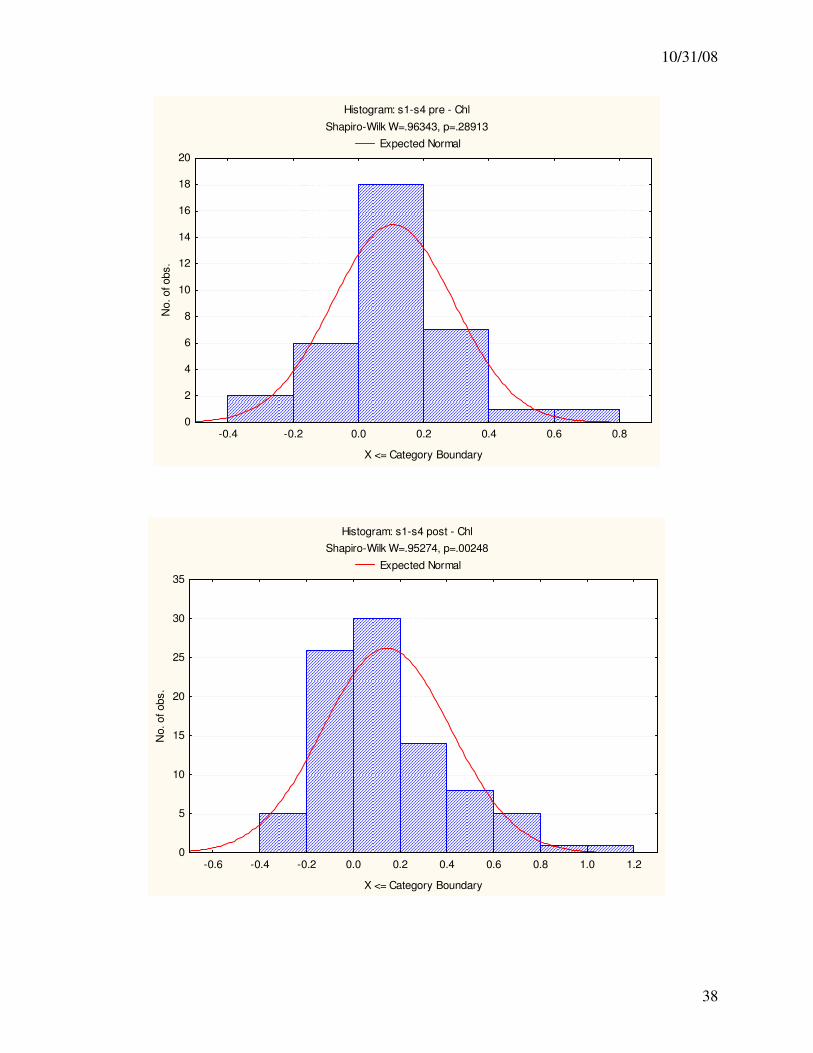
10/31/08
38
Histogram: s1-s4 pre - Chl
Shapiro-Wilk W=.96343, p=.28913
Expected Normal
-0.4 -0.2 0.0 0.2 0.4 0.6 0.8
X <= Category Boundary
0
2
4
6
8
10
12
14
16
18
20N
o. of obs.
Histogram: s1-s4 post - Chl
Shapiro-Wilk W=.95274, p=.00248
Expected Normal
-0.6 -0.4 -0.2 0.0 0.2 0.4 0.6 0.8 1.0 1.2
X <= Category Boundary
0
5
10
15
20
25
30
35
No. of obs.
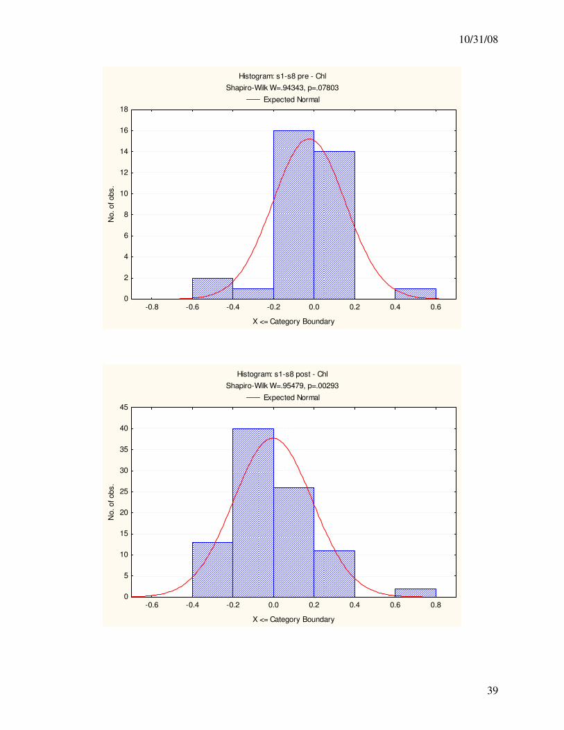
10/31/08
39
Histogram: s1-s8 pre - Chl
Shapiro-Wilk W=.94343, p=.07803
Expected Normal
-0.8 -0.6 -0.4 -0.2 0.0 0.2 0.4 0.6
X <= Category Boundary
0
2
4
6
8
10
12
14
16
18N
o. of obs.
Histogram: s1-s8 post - Chl
Shapiro-Wilk W=.95479, p=.00293
Expected Normal
-0.6 -0.4 -0.2 0.0 0.2 0.4 0.6 0.8
X <= Category Boundary
0
5
10
15
20
25
30
35
40
45
No. of obs.
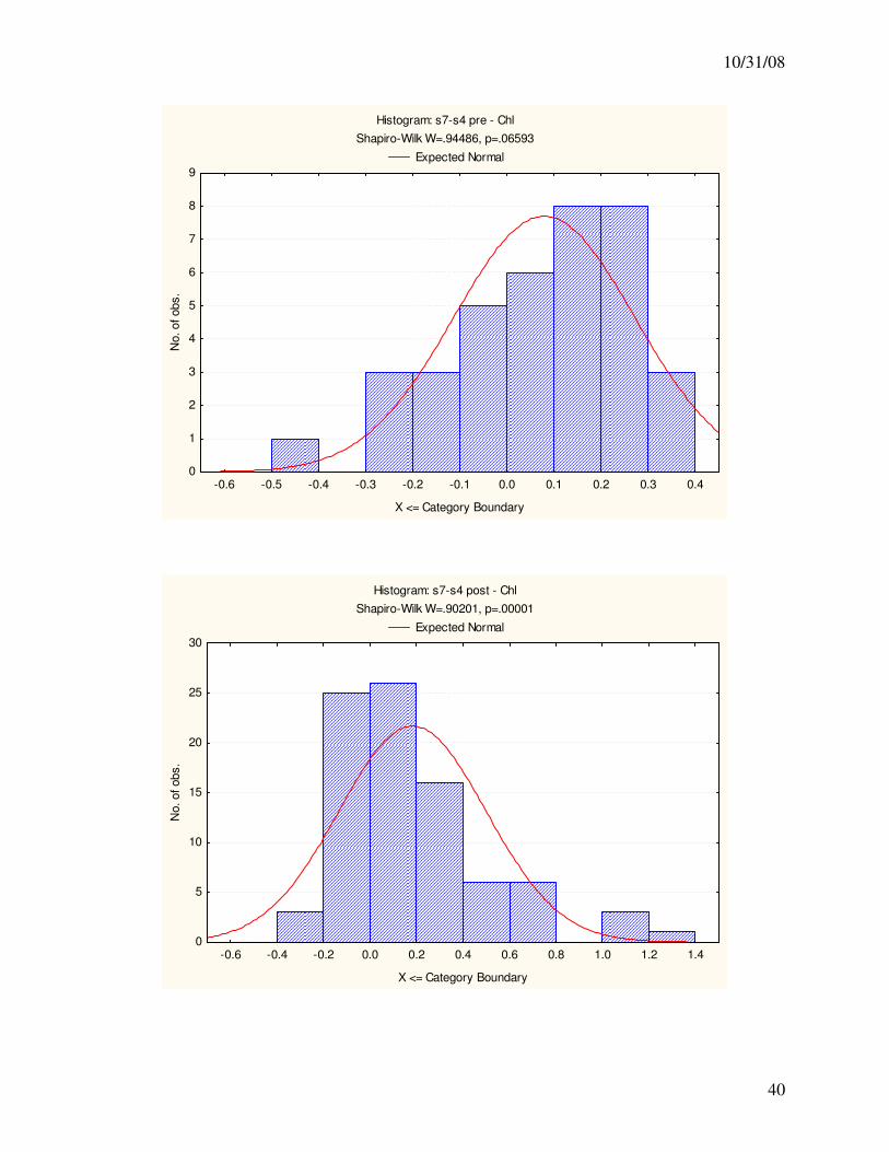
10/31/08
40
Histogram: s7-s4 pre - Chl
Shapiro-Wilk W=.94486, p=.06593
Expected Normal
-0.6 -0.5 -0.4 -0.3 -0.2 -0.1 0.0 0.1 0.2 0.3 0.4
X <= Category Boundary
0
1
2
3
4
5
6
7
8
9N
o. of obs.
Histogram: s7-s4 post - Chl
Shapiro-Wilk W=.90201, p=.00001
Expected Normal
-0.6 -0.4 -0.2 0.0 0.2 0.4 0.6 0.8 1.0 1.2 1.4
X <= Category Boundary
0
5
10
15
20
25
30
No. of obs.
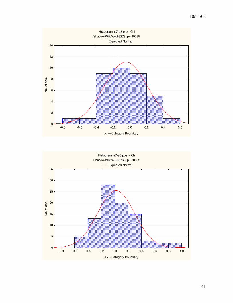
10/31/08
41
Histogram: s7-s8 pre - Chl
Shapiro-Wilk W=.99273, p=.99725
Expected Normal
-0.8 -0.6 -0.4 -0.2 0.0 0.2 0.4 0.6
X <= Category Boundary
0
2
4
6
8
10
12
14N
o. of obs.
Histogram: s7-s8 post - Chl
Shapiro-Wilk W=.95766, p=.00582
Expected Normal
-0.8 -0.6 -0.4 -0.2 0.0 0.2 0.4 0.6 0.8 1.0
X <= Category Boundary
0
5
10
15
20
25
30
35
No. of obs.
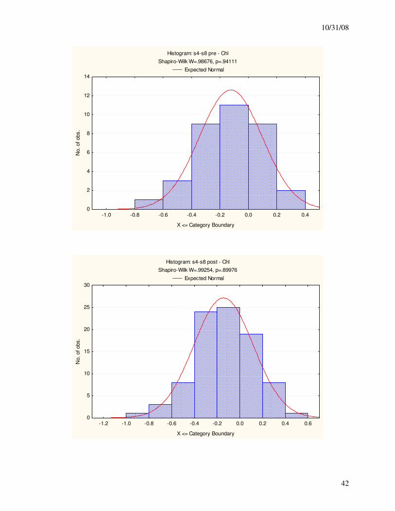
10/31/08
42
Histogram: s4-s8 pre - Chl
Shapiro-Wilk W=.98676, p=.94111
Expected Normal
-1.0 -0.8 -0.6 -0.4 -0.2 0.0 0.2 0.4
X <= Category Boundary
0
2
4
6
8
10
12
14N
o. of obs.
Histogram: s4-s8 post - Chl
Shapiro-Wilk W=.99254, p=.89976
Expected Normal
-1.2 -1.0 -0.8 -0.6 -0.4 -0.2 0.0 0.2 0.4 0.6
X <= Category Boundary
0
5
10
15
20
25
30
No. of obs.
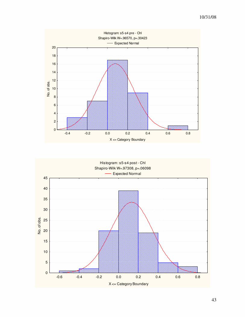
10/31/08
43
Histogram: s5-s4 pre - Chl
Shapiro-Wilk W=.96570, p=.30423
Expected Normal
-0.4 -0.2 0.0 0.2 0.4 0.6 0.8
X <= Category Boundary
0
2
4
6
8
10
12
14
16
18
20N
o. of obs.
Histogram: s5-s4 post - Chl
Shapiro-Wilk W=.97308, p=.06098
Expected Normal
-0.6 -0.4 -0.2 0.0 0.2 0.4 0.6 0.8
X <= Category Boundary
0
5
10
15
20
25
30
35
40
45
No
. o
f o
bs.
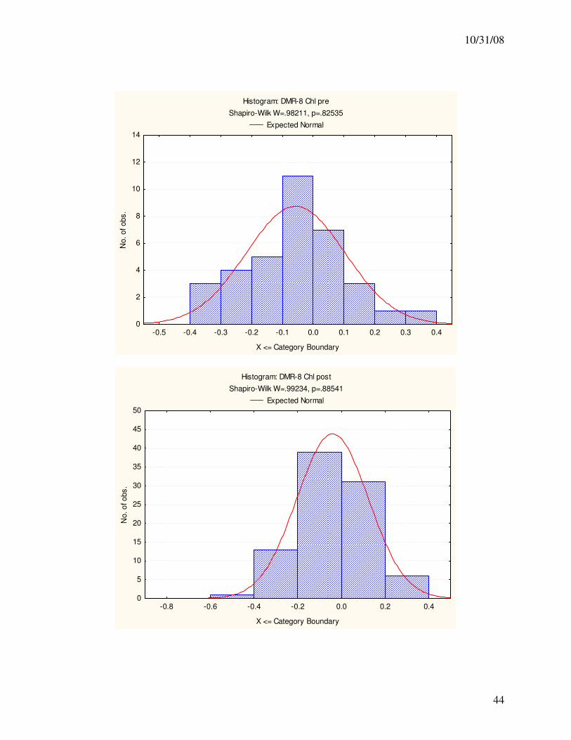
10/31/08
44
Histogram: DMR-8 Chl pre
Shapiro-Wilk W=.98211, p=.82535
Expected Normal
-0.5 -0.4 -0.3 -0.2 -0.1 0.0 0.1 0.2 0.3 0.4
X <= Category Boundary
0
2
4
6
8
10
12
14
No.
of
ob
s.
Histogram: DMR-8 Chl post
Shapiro-Wilk W=.99234, p=.88541
Expected Normal
-0.8 -0.6 -0.4 -0.2 0.0 0.2 0.4
X <= Category Boundary
0
5
10
15
20
25
30
35
40
45
50
No
. o
f o
bs
.
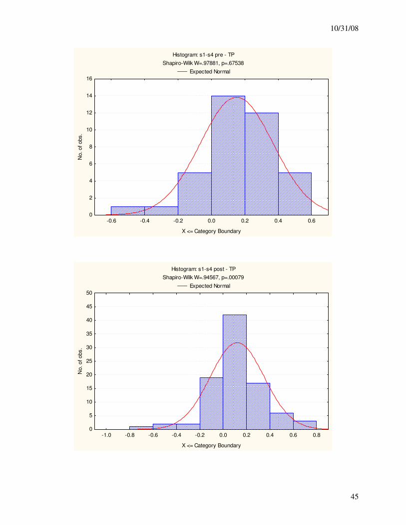
10/31/08
45
Histogram: s1-s4 pre - TP
Shapiro-Wilk W=.97881, p=.67538
Expected Normal
-0.6 -0.4 -0.2 0.0 0.2 0.4 0.6
X <= Category Boundary
0
2
4
6
8
10
12
14
16N
o. of obs.
Histogram: s1-s4 post - TP
Shapiro-Wilk W=.94567, p=.00079
Expected Normal
-1.0 -0.8 -0.6 -0.4 -0.2 0.0 0.2 0.4 0.6 0.8
X <= Category Boundary
0
5
10
15
20
25
30
35
40
45
50
No. of obs.
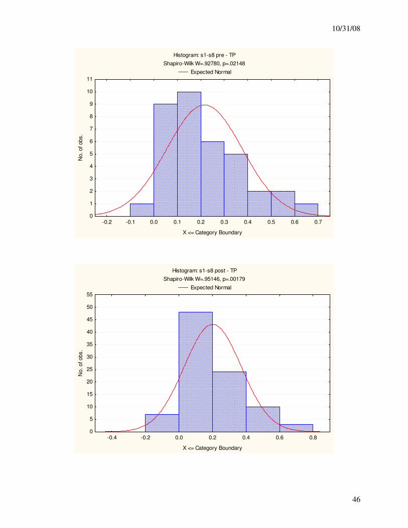
10/31/08
46
Histogram: s1-s8 pre - TP
Shapiro-Wilk W=.92780, p=.02148
Expected Normal
-0.2 -0.1 0.0 0.1 0.2 0.3 0.4 0.5 0.6 0.7
X <= Category Boundary
0
1
2
3
4
5
6
7
8
9
10
11N
o. of obs.
Histogram: s1-s8 post - TP
Shapiro-Wilk W=.95146, p=.00179
Expected Normal
-0.4 -0.2 0.0 0.2 0.4 0.6 0.8
X <= Category Boundary
0
5
10
15
20
25
30
35
40
45
50
55
No. of obs.
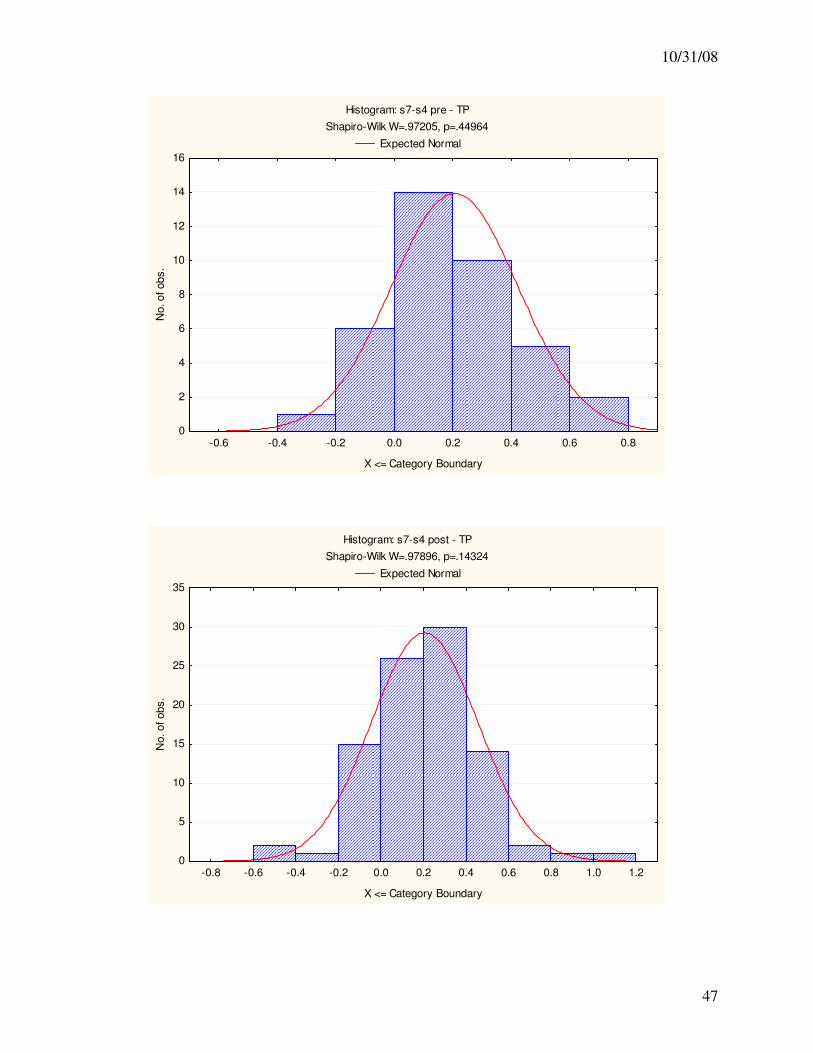
10/31/08
47
Histogram: s7-s4 pre - TP
Shapiro-Wilk W=.97205, p=.44964
Expected Normal
-0.6 -0.4 -0.2 0.0 0.2 0.4 0.6 0.8
X <= Category Boundary
0
2
4
6
8
10
12
14
16N
o. of obs.
Histogram: s7-s4 post - TP
Shapiro-Wilk W=.97896, p=.14324
Expected Normal
-0.8 -0.6 -0.4 -0.2 0.0 0.2 0.4 0.6 0.8 1.0 1.2
X <= Category Boundary
0
5
10
15
20
25
30
35
No. of obs.
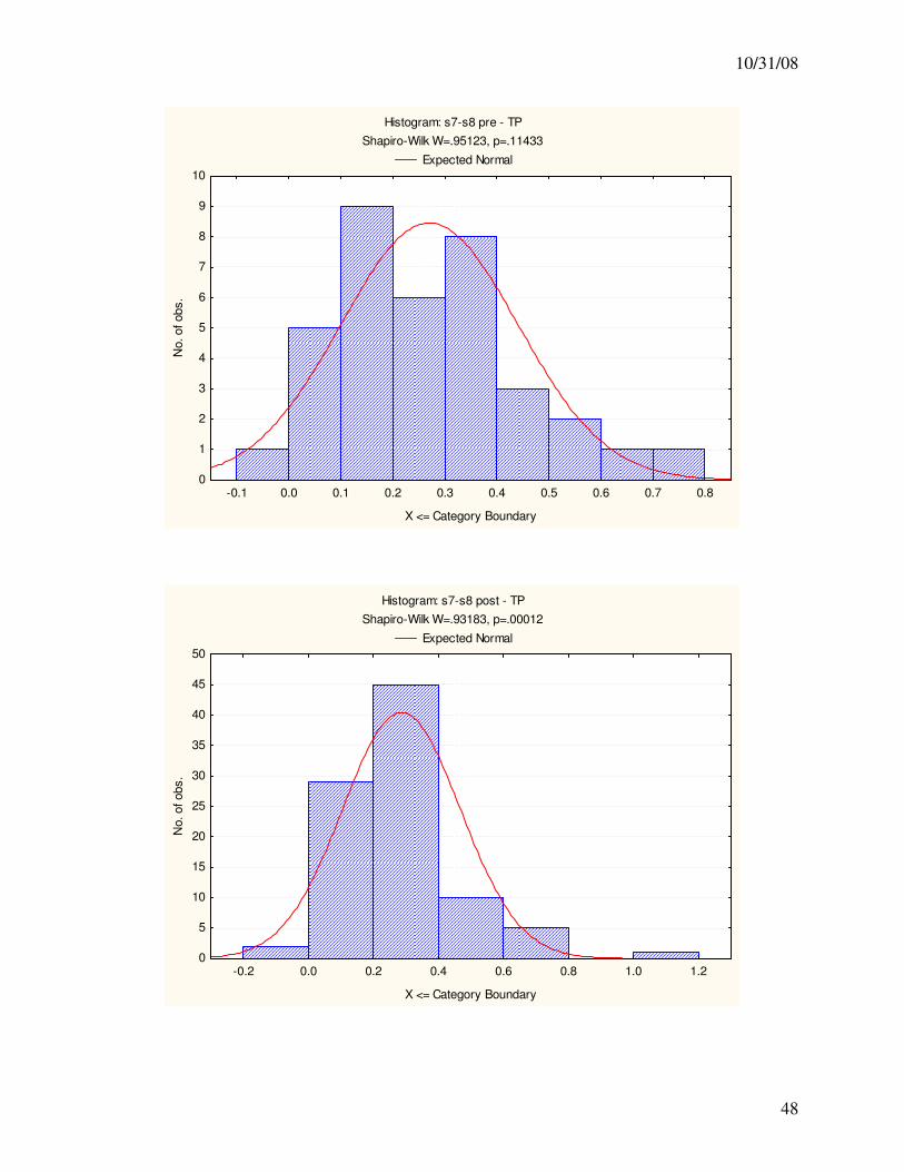
10/31/08
48
Histogram: s7-s8 pre - TP
Shapiro-Wilk W=.95123, p=.11433
Expected Normal
-0.1 0.0 0.1 0.2 0.3 0.4 0.5 0.6 0.7 0.8
X <= Category Boundary
0
1
2
3
4
5
6
7
8
9
10N
o. of obs.
Histogram: s7-s8 post - TP
Shapiro-Wilk W=.93183, p=.00012
Expected Normal
-0.2 0.0 0.2 0.4 0.6 0.8 1.0 1.2
X <= Category Boundary
0
5
10
15
20
25
30
35
40
45
50
No. of obs.
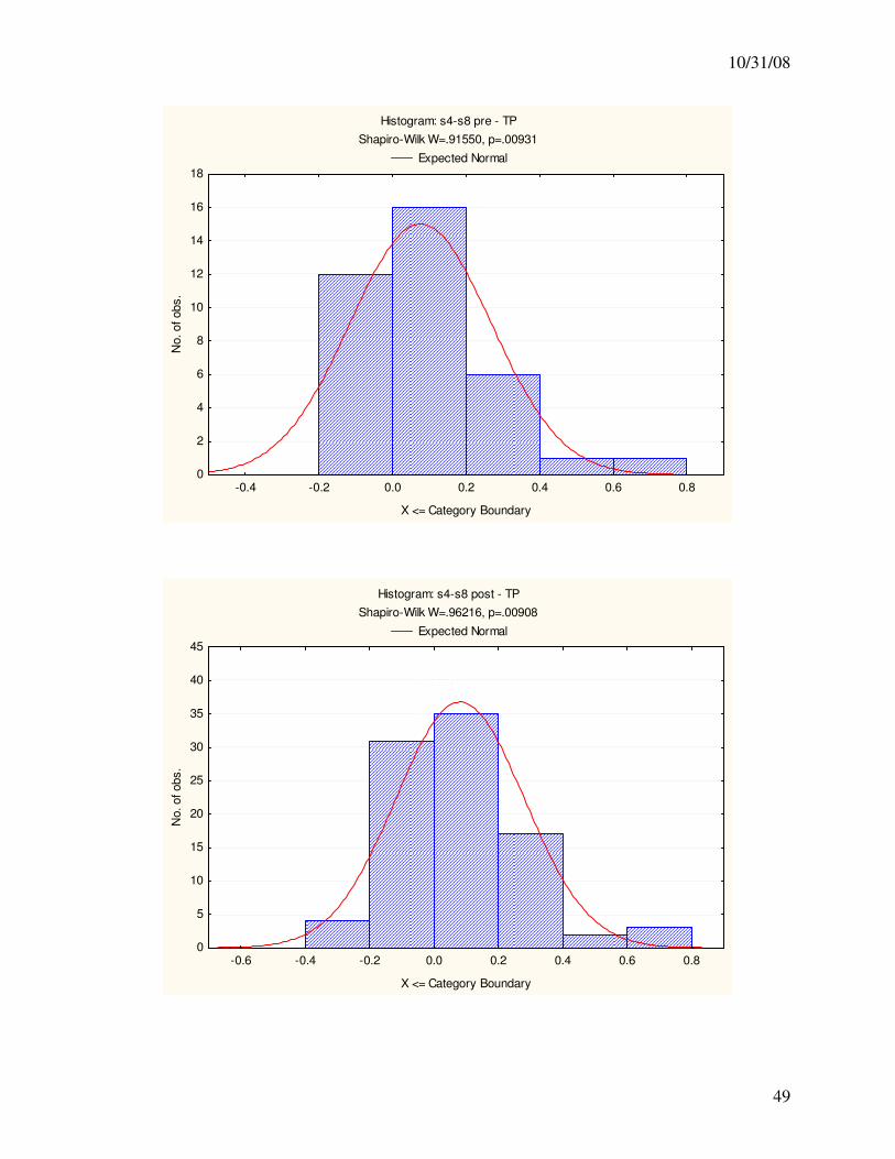
10/31/08
49
Histogram: s4-s8 pre - TP
Shapiro-Wilk W=.91550, p=.00931
Expected Normal
-0.4 -0.2 0.0 0.2 0.4 0.6 0.8
X <= Category Boundary
0
2
4
6
8
10
12
14
16
18N
o. of obs.
Histogram: s4-s8 post - TP
Shapiro-Wilk W=.96216, p=.00908
Expected Normal
-0.6 -0.4 -0.2 0.0 0.2 0.4 0.6 0.8
X <= Category Boundary
0
5
10
15
20
25
30
35
40
45
No. of obs.
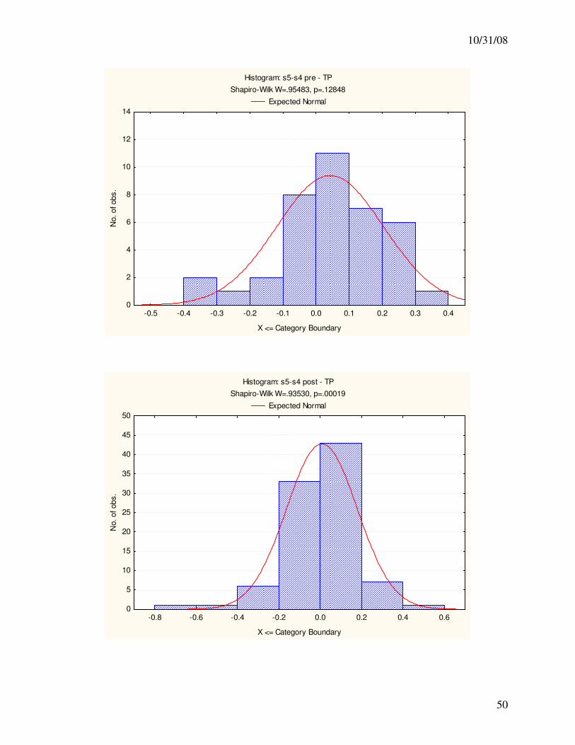
10/31/08
50
Histogram: s5-s4 pre - TP
Shapiro-Wilk W=.95483, p=.12848
Expected Normal
-0.5 -0.4 -0.3 -0.2 -0.1 0.0 0.1 0.2 0.3 0.4
X <= Category Boundary
0
2
4
6
8
10
12
14N
o. of obs.
Histogram: s5-s4 post - TP
Shapiro-Wilk W=.93530, p=.00019
Expected Normal
-0.8 -0.6 -0.4 -0.2 0.0 0.2 0.4 0.6
X <= Category Boundary
0
5
10
15
20
25
30
35
40
45
50
No. of obs.
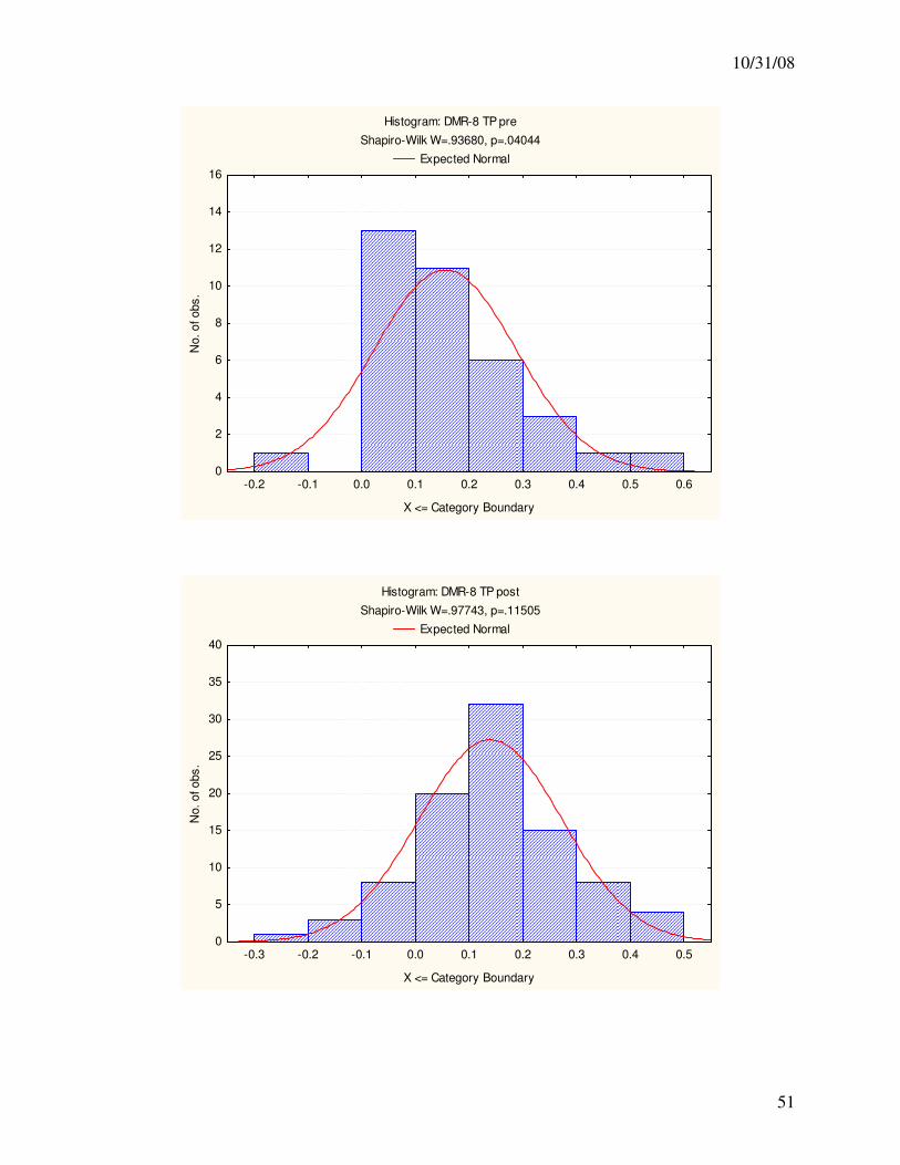
10/31/08
51
Histogram: DMR-8 TP pre
Shapiro-Wilk W=.93680, p=.04044
Expected Normal
-0.2 -0.1 0.0 0.1 0.2 0.3 0.4 0.5 0.6
X <= Category Boundary
0
2
4
6
8
10
12
14
16
No.
of o
bs
.
Histogram: DMR-8 TP post
Shapiro-Wilk W=.97743, p=.11505
Expected Normal
-0.3 -0.2 -0.1 0.0 0.1 0.2 0.3 0.4 0.5
X <= Category Boundary
0
5
10
15
20
25
30
35
40
No.
of o
bs
.
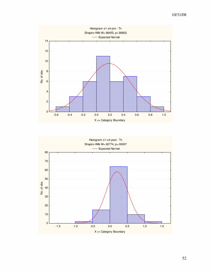
10/31/08
52
Histogram: s1-s4 pre - Tn
Shapiro-Wilk W=.98455, p=.86802
Expected Normal
-0.6 -0.4 -0.2 0.0 0.2 0.4 0.6 0.8 1.0
X <= Category Boundary
0
2
4
6
8
10
12
14N
o. of obs.
Histogram: s1-s4 post - Tn
Shapiro-Wilk W=.92774, p=.00007
Expected Normal
-1.5 -1.0 -0.5 0.0 0.5 1.0 1.5
X <= Category Boundary
0
10
20
30
40
50
60
70
80
No. of obs.
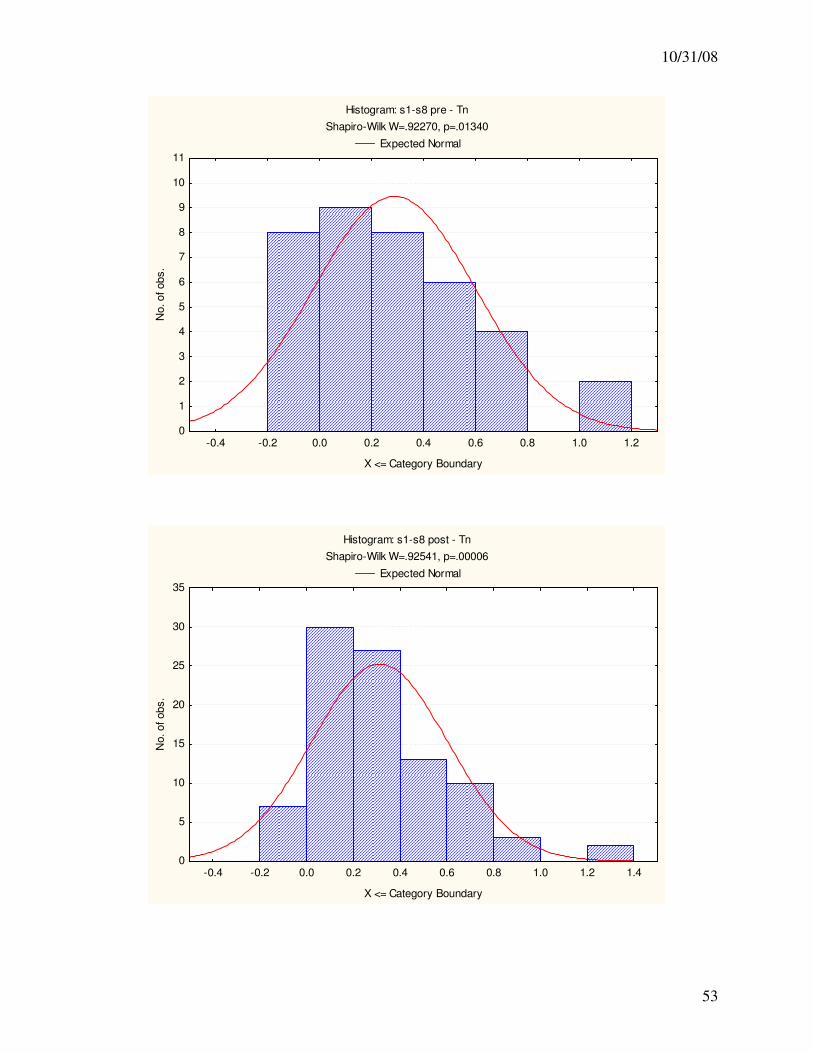
10/31/08
53
Histogram: s1-s8 pre - Tn
Shapiro-Wilk W=.92270, p=.01340
Expected Normal
-0.4 -0.2 0.0 0.2 0.4 0.6 0.8 1.0 1.2
X <= Category Boundary
0
1
2
3
4
5
6
7
8
9
10
11N
o. of obs.
Histogram: s1-s8 post - Tn
Shapiro-Wilk W=.92541, p=.00006
Expected Normal
-0.4 -0.2 0.0 0.2 0.4 0.6 0.8 1.0 1.2 1.4
X <= Category Boundary
0
5
10
15
20
25
30
35
No. of obs.
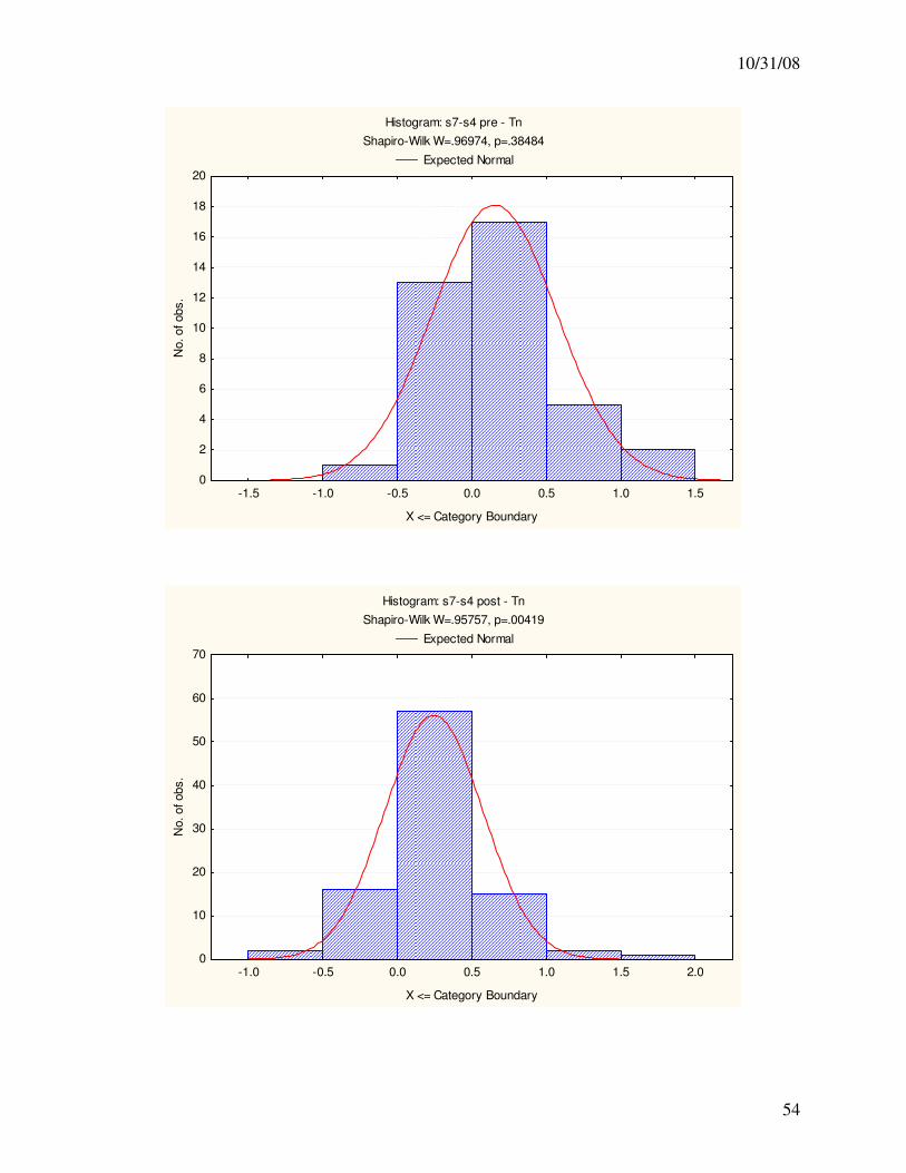
10/31/08
54
Histogram: s7-s4 pre - Tn
Shapiro-Wilk W=.96974, p=.38484
Expected Normal
-1.5 -1.0 -0.5 0.0 0.5 1.0 1.5
X <= Category Boundary
0
2
4
6
8
10
12
14
16
18
20N
o. of obs.
Histogram: s7-s4 post - Tn
Shapiro-Wilk W=.95757, p=.00419
Expected Normal
-1.0 -0.5 0.0 0.5 1.0 1.5 2.0
X <= Category Boundary
0
10
20
30
40
50
60
70
No. of obs.
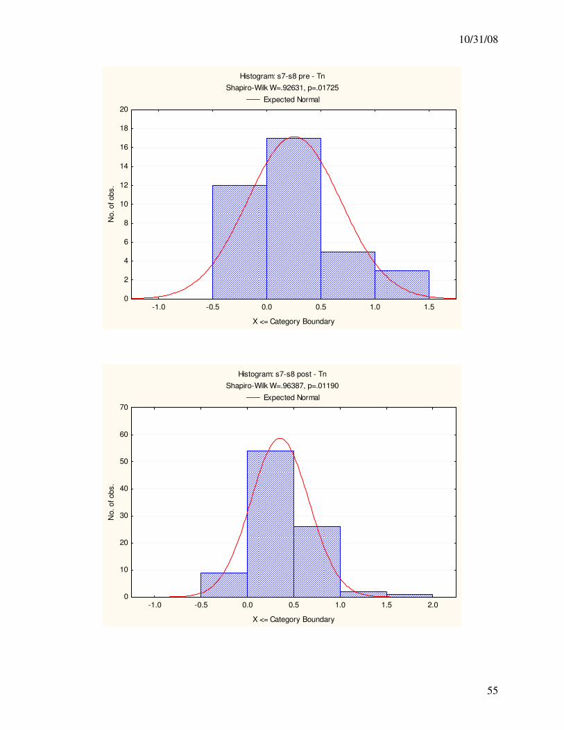
10/31/08
55
Histogram: s7-s8 pre - Tn
Shapiro-Wilk W=.92631, p=.01725
Expected Normal
-1.0 -0.5 0.0 0.5 1.0 1.5
X <= Category Boundary
0
2
4
6
8
10
12
14
16
18
20N
o. of obs.
Histogram: s7-s8 post - Tn
Shapiro-Wilk W=.96387, p=.01190
Expected Normal
-1.0 -0.5 0.0 0.5 1.0 1.5 2.0
X <= Category Boundary
0
10
20
30
40
50
60
70
No. of obs.
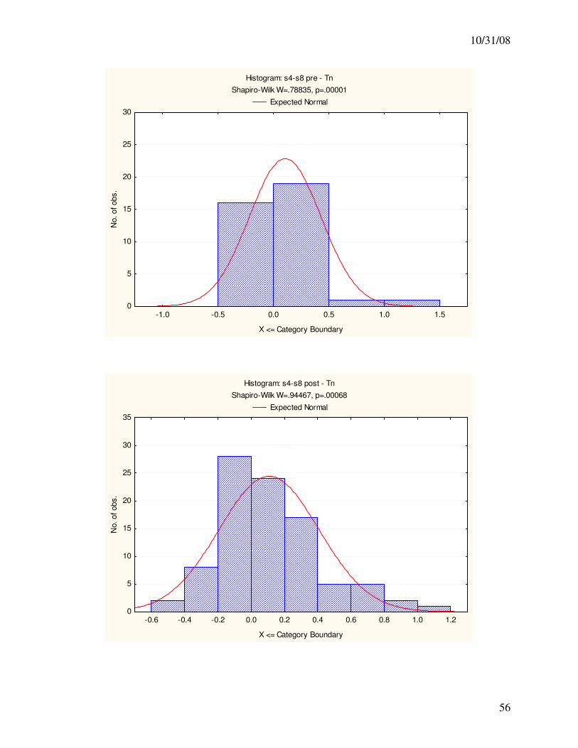
10/31/08
56
Histogram: s4-s8 pre - Tn
Shapiro-Wilk W=.78835, p=.00001
Expected Normal
-1.0 -0.5 0.0 0.5 1.0 1.5
X <= Category Boundary
0
5
10
15
20
25
30N
o. of obs.
Histogram: s4-s8 post - Tn
Shapiro-Wilk W=.94467, p=.00068
Expected Normal
-0.6 -0.4 -0.2 0.0 0.2 0.4 0.6 0.8 1.0 1.2
X <= Category Boundary
0
5
10
15
20
25
30
35
No. of obs.
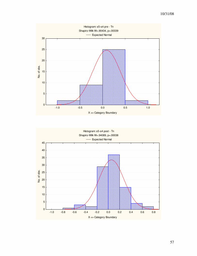
10/31/08
57
Histogram: s5-s4 pre - Tn
Shapiro-Wilk W=.90434, p=.00339
Expected Normal
-1.0 -0.5 0.0 0.5 1.0
X <= Category Boundary
0
5
10
15
20
25
30N
o. of obs.
Histogram: s5-s4 post - Tn
Shapiro-Wilk W=.94089, p=.00038
Expected Normal
-1.0 -0.8 -0.6 -0.4 -0.2 0.0 0.2 0.4 0.6 0.8
X <= Category Boundary
0
5
10
15
20
25
30
35
40
45
No. of obs.
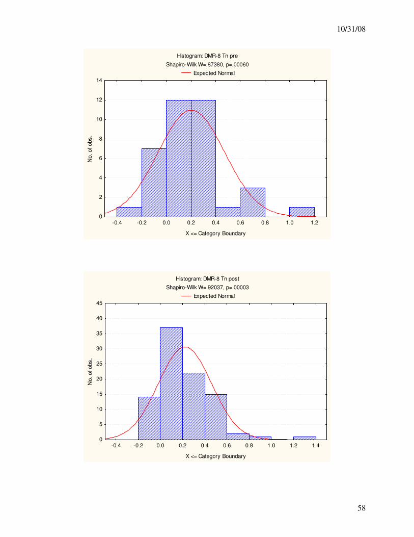
10/31/08
58
Histogram: DMR-8 Tn pre
Shapiro-Wilk W=.87380, p=.00060
Expected Normal
-0.4 -0.2 0.0 0.2 0.4 0.6 0.8 1.0 1.2
X <= Category Boundary
0
2
4
6
8
10
12
14
No
. o
f o
bs
.
Histogram: DMR-8 Tn post
Shapiro-Wilk W=.92037, p=.00003
Expected Normal
-0.4 -0.2 0.0 0.2 0.4 0.6 0.8 1.0 1.2 1.4
X <= Category Boundary
0
5
10
15
20
25
30
35
40
45
No
. o
f o
bs
.

10/31/08
59
Appendix 2 - Independence
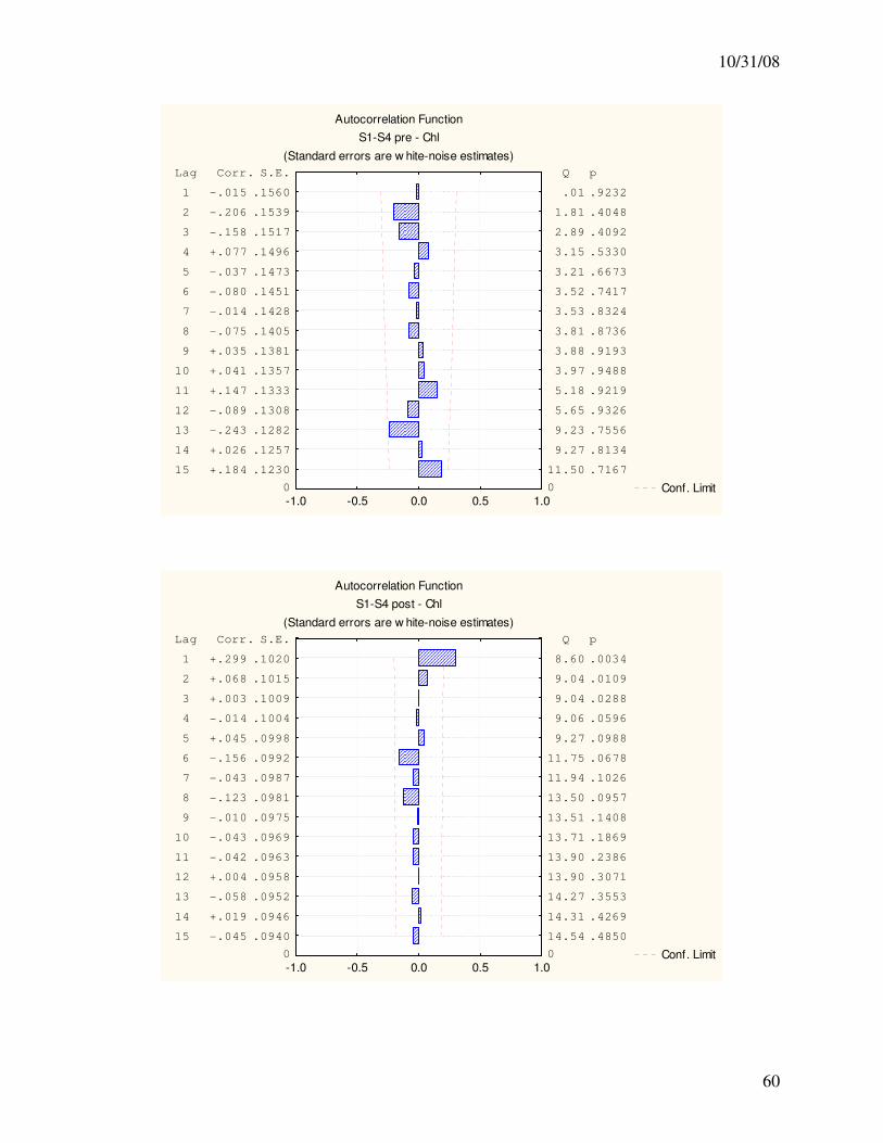
10/31/08
60
Autocorrelation Function
S1-S4 pre - Chl
(Standard errors are w hite-noise estimates)
Conf. Limit-1.0 -0.5 0.0 0.5 1.00
15 +.184 .1230
14 +.026 .1257
13 -.243 .1282
12 -.089 .1308
11 +.147 .1333
10 +.041 .1357
9 +.035 .1381
8 -.075 .1405
7 -.014 .1428
6 -.080 .1451
5 -.037 .1473
4 +.077 .1496
3 -.158 .1517
2 -.206 .1539
1 -.015 .1560
Lag Corr. S.E.
0
11.50 .7167
9.27 .8134
9.23 .7556
5.65 .9326
5.18 .9219
3.97 .9488
3.88 .9193
3.81 .8736
3.53 .8324
3.52 .7417
3.21 .6673
3.15 .5330
2.89 .4092
1.81 .4048
.01 .9232
Q p
Autocorrelation Function
S1-S4 post - Chl
(Standard errors are w hite-noise estimates)
Conf. Limit-1.0 -0.5 0.0 0.5 1.00
15 -.045 .0940
14 +.019 .0946
13 -.058 .0952
12 +.004 .0958
11 -.042 .0963
10 -.043 .0969
9 -.010 .0975
8 -.123 .0981
7 -.043 .0987
6 -.156 .0992
5 +.045 .0998
4 -.014 .1004
3 +.003 .1009
2 +.068 .1015
1 +.299 .1020
Lag Corr. S.E.
0
14.54 .4850
14.31 .4269
14.27 .3553
13.90 .3071
13.90 .2386
13.71 .1869
13.51 .1408
13.50 .0957
11.94 .1026
11.75 .0678
9.27 .0988
9.06 .0596
9.04 .0288
9.04 .0109
8.60 .0034
Q p
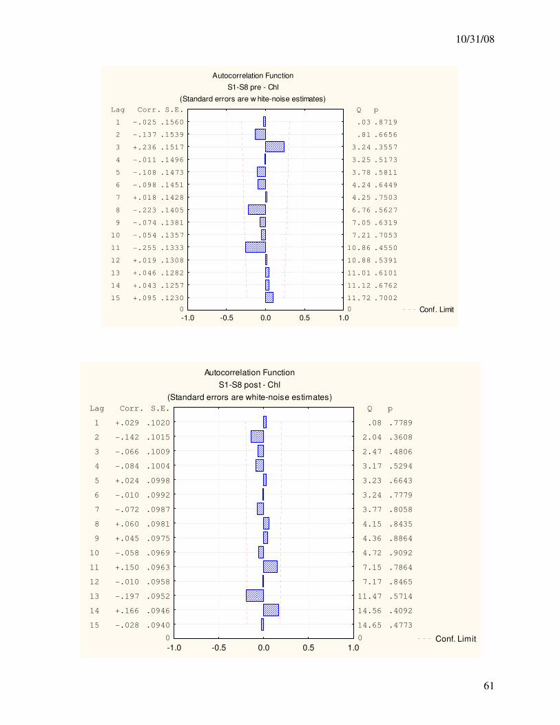
10/31/08
61
Autocorrelation Function
S1-S8 pre - Chl
(Standard errors are w hite-noise estimates)
Conf. Limit-1.0 -0.5 0.0 0.5 1.00
15 +.095 .1230
14 +.043 .1257
13 +.046 .1282
12 +.019 .1308
11 -.255 .1333
10 -.054 .1357
9 -.074 .1381
8 -.223 .1405
7 +.018 .1428
6 -.098 .1451
5 -.108 .1473
4 -.011 .1496
3 +.236 .1517
2 -.137 .1539
1 -.025 .1560
Lag Corr. S.E.
0
11.72 .7002
11.12 .6762
11.01 .6101
10.88 .5391
10.86 .4550
7.21 .7053
7.05 .6319
6.76 .5627
4.25 .7503
4.24 .6449
3.78 .5811
3.25 .5173
3.24 .3557
.81 .6656
.03 .8719
Q p
Autocorrelation Function
S1-S8 post - Chl
(Standard errors are white-noise estimates)
Conf. Limit-1.0 -0.5 0.0 0.5 1.0
0
15 -.028 .0940
14 +.166 .0946
13 -.197 .0952
12 -.010 .0958
11 +.150 .0963
10 -.058 .0969
9 +.045 .0975
8 +.060 .0981
7 -.072 .0987
6 -.010 .0992
5 +.024 .0998
4 -.084 .1004
3 -.066 .1009
2 -.142 .1015
1 +.029 .1020
Lag Corr. S.E.
0
14.65 .4773
14.56 .4092
11.47 .5714
7.17 .8465
7.15 .7864
4.72 .9092
4.36 .8864
4.15 .8435
3.77 .8058
3.24 .7779
3.23 .6643
3.17 .5294
2.47 .4806
2.04 .3608
.08 .7789
Q p
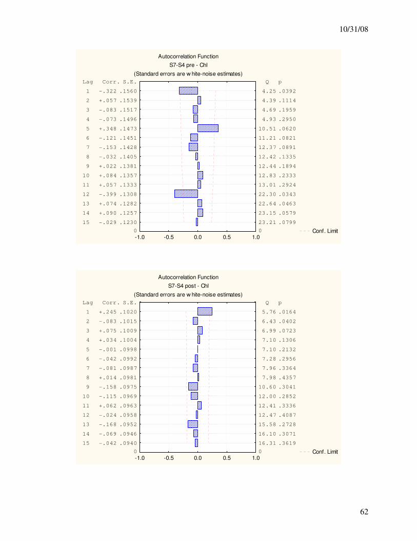
10/31/08
62
Autocorrelation Function
S7-S4 pre - Chl
(Standard errors are w hite-noise estimates)
Conf. Limit-1.0 -0.5 0.0 0.5 1.00
15 -.029 .1230
14 +.090 .1257
13 +.074 .1282
12 -.399 .1308
11 +.057 .1333
10 +.084 .1357
9 +.022 .1381
8 -.032 .1405
7 -.153 .1428
6 -.121 .1451
5 +.348 .1473
4 -.073 .1496
3 -.083 .1517
2 +.057 .1539
1 -.322 .1560
Lag Corr. S.E.
0
23.21 .0799
23.15 .0579
22.64 .0463
22.30 .0343
13.01 .2924
12.83 .2333
12.44 .1894
12.42 .1335
12.37 .0891
11.21 .0821
10.51 .0620
4.93 .2950
4.69 .1959
4.39 .1114
4.25 .0392
Q p
Autocorrelation Function
S7-S4 post - Chl
(Standard errors are w hite-noise estimates)
Conf. Limit-1.0 -0.5 0.0 0.5 1.00
15 -.042 .0940
14 -.069 .0946
13 -.168 .0952
12 -.024 .0958
11 +.062 .0963
10 -.115 .0969
9 -.158 .0975
8 +.014 .0981
7 -.081 .0987
6 -.042 .0992
5 -.001 .0998
4 +.034 .1004
3 +.075 .1009
2 -.083 .1015
1 +.245 .1020
Lag Corr. S.E.
0
16.31 .3619
16.10 .3071
15.58 .2728
12.47 .4087
12.41 .3336
12.00 .2852
10.60 .3041
7.98 .4357
7.96 .3364
7.28 .2956
7.10 .2132
7.10 .1306
6.99 .0723
6.43 .0402
5.76 .0164
Q p
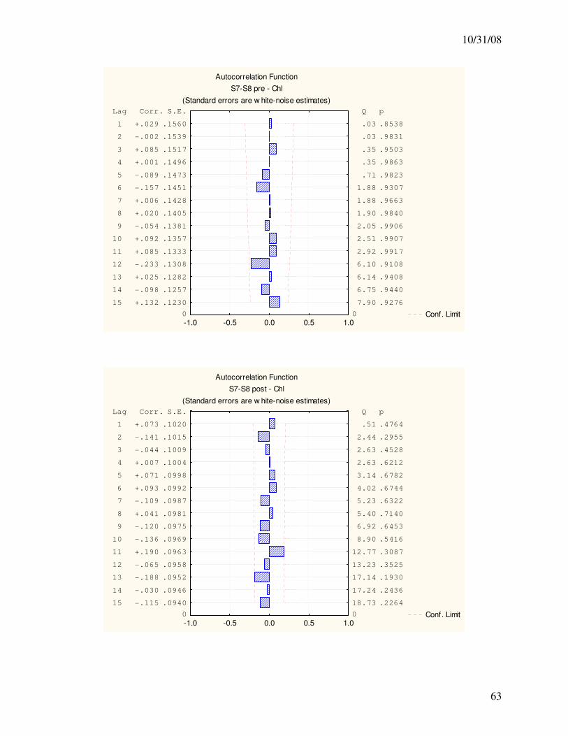
10/31/08
63
Autocorrelation Function
S7-S8 pre - Chl
(Standard errors are w hite-noise estimates)
Conf. Limit-1.0 -0.5 0.0 0.5 1.00
15 +.132 .1230
14 -.098 .1257
13 +.025 .1282
12 -.233 .1308
11 +.085 .1333
10 +.092 .1357
9 -.054 .1381
8 +.020 .1405
7 +.006 .1428
6 -.157 .1451
5 -.089 .1473
4 +.001 .1496
3 +.085 .1517
2 -.002 .1539
1 +.029 .1560
Lag Corr. S.E.
0
7.90 .9276
6.75 .9440
6.14 .9408
6.10 .9108
2.92 .9917
2.51 .9907
2.05 .9906
1.90 .9840
1.88 .9663
1.88 .9307
.71 .9823
.35 .9863
.35 .9503
.03 .9831
.03 .8538
Q p
Autocorrelation Function
S7-S8 post - Chl
(Standard errors are w hite-noise estimates)
Conf. Limit-1.0 -0.5 0.0 0.5 1.00
15 -.115 .0940
14 -.030 .0946
13 -.188 .0952
12 -.065 .0958
11 +.190 .0963
10 -.136 .0969
9 -.120 .0975
8 +.041 .0981
7 -.109 .0987
6 +.093 .0992
5 +.071 .0998
4 +.007 .1004
3 -.044 .1009
2 -.141 .1015
1 +.073 .1020
Lag Corr. S.E.
0
18.73 .2264
17.24 .2436
17.14 .1930
13.23 .3525
12.77 .3087
8.90 .5416
6.92 .6453
5.40 .7140
5.23 .6322
4.02 .6744
3.14 .6782
2.63 .6212
2.63 .4528
2.44 .2955
.51 .4764
Q p
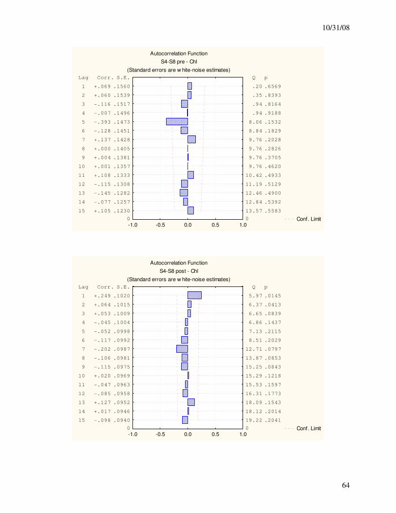
10/31/08
64
Autocorrelation Function
S4-S8 pre - Chl
(Standard errors are w hite-noise estimates)
Conf. Limit-1.0 -0.5 0.0 0.5 1.00
15 +.105 .1230
14 -.077 .1257
13 -.145 .1282
12 -.115 .1308
11 +.108 .1333
10 +.001 .1357
9 +.004 .1381
8 +.000 .1405
7 +.137 .1428
6 -.128 .1451
5 -.393 .1473
4 -.007 .1496
3 -.116 .1517
2 +.060 .1539
1 +.069 .1560
Lag Corr. S.E.
0
13.57 .5583
12.84 .5392
12.46 .4900
11.19 .5129
10.42 .4933
9.76 .4620
9.76 .3705
9.76 .2826
9.76 .2028
8.84 .1829
8.06 .1532
.94 .9188
.94 .8164
.35 .8393
.20 .6569
Q p
Autocorrelation Function
S4-S8 post - Chl
(Standard errors are w hite-noise estimates)
Conf. Limit-1.0 -0.5 0.0 0.5 1.00
15 -.098 .0940
14 +.017 .0946
13 +.127 .0952
12 -.085 .0958
11 -.047 .0963
10 +.020 .0969
9 -.115 .0975
8 -.106 .0981
7 -.202 .0987
6 -.117 .0992
5 -.052 .0998
4 -.045 .1004
3 +.053 .1009
2 +.064 .1015
1 +.249 .1020
Lag Corr. S.E.
0
19.22 .2041
18.12 .2014
18.09 .1543
16.31 .1773
15.53 .1597
15.29 .1218
15.25 .0843
13.87 .0853
12.71 .0797
8.51 .2029
7.13 .2115
6.86 .1437
6.65 .0839
6.37 .0413
5.97 .0145
Q p
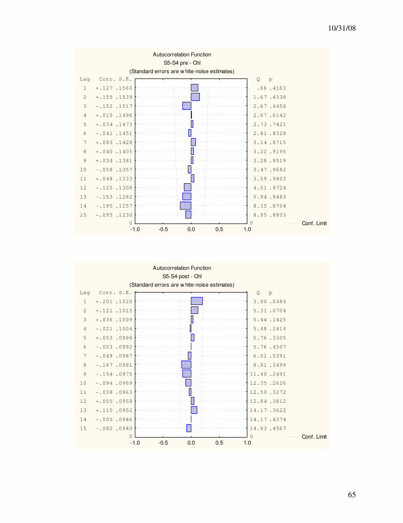
10/31/08
65
Autocorrelation Function
S5-S4 pre - Chl
(Standard errors are w hite-noise estimates)
Conf. Limit-1.0 -0.5 0.0 0.5 1.00
15 -.095 .1230
14 -.195 .1257
13 -.153 .1282
12 -.125 .1308
11 +.048 .1333
10 -.058 .1357
9 +.034 .1381
8 +.040 .1405
7 +.083 .1428
6 -.041 .1451
5 +.034 .1473
4 +.010 .1496
3 -.152 .1517
2 +.155 .1539
1 +.127 .1560
Lag Corr. S.E.
0
8.95 .8803
8.35 .8704
5.94 .9483
4.51 .9724
3.59 .9803
3.47 .9682
3.28 .9519
3.22 .9195
3.14 .8715
2.81 .8328
2.73 .7421
2.67 .6142
2.67 .4458
1.67 .4338
.66 .4163
Q p
Autocorrelation Function
S5-S4 post - Chl
(Standard errors are w hite-noise estimates)
Conf. Limit-1.0 -0.5 0.0 0.5 1.00
15 -.082 .0940
14 -.000 .0946
13 +.110 .0952
12 +.055 .0958
11 -.038 .0963
10 -.094 .0969
9 -.154 .0975
8 -.167 .0981
7 -.049 .0987
6 -.003 .0992
5 +.053 .0998
4 -.021 .1004
3 +.036 .1009
2 +.121 .1015
1 +.201 .1020
Lag Corr. S.E.
0
14.93 .4567
14.17 .4374
14.17 .3622
12.84 .3812
12.50 .3272
12.35 .2626
11.40 .2491
8.91 .3499
6.01 .5391
5.76 .4507
5.76 .3305
5.48 .2414
5.44 .1425
5.31 .0704
3.90 .0484
Q p
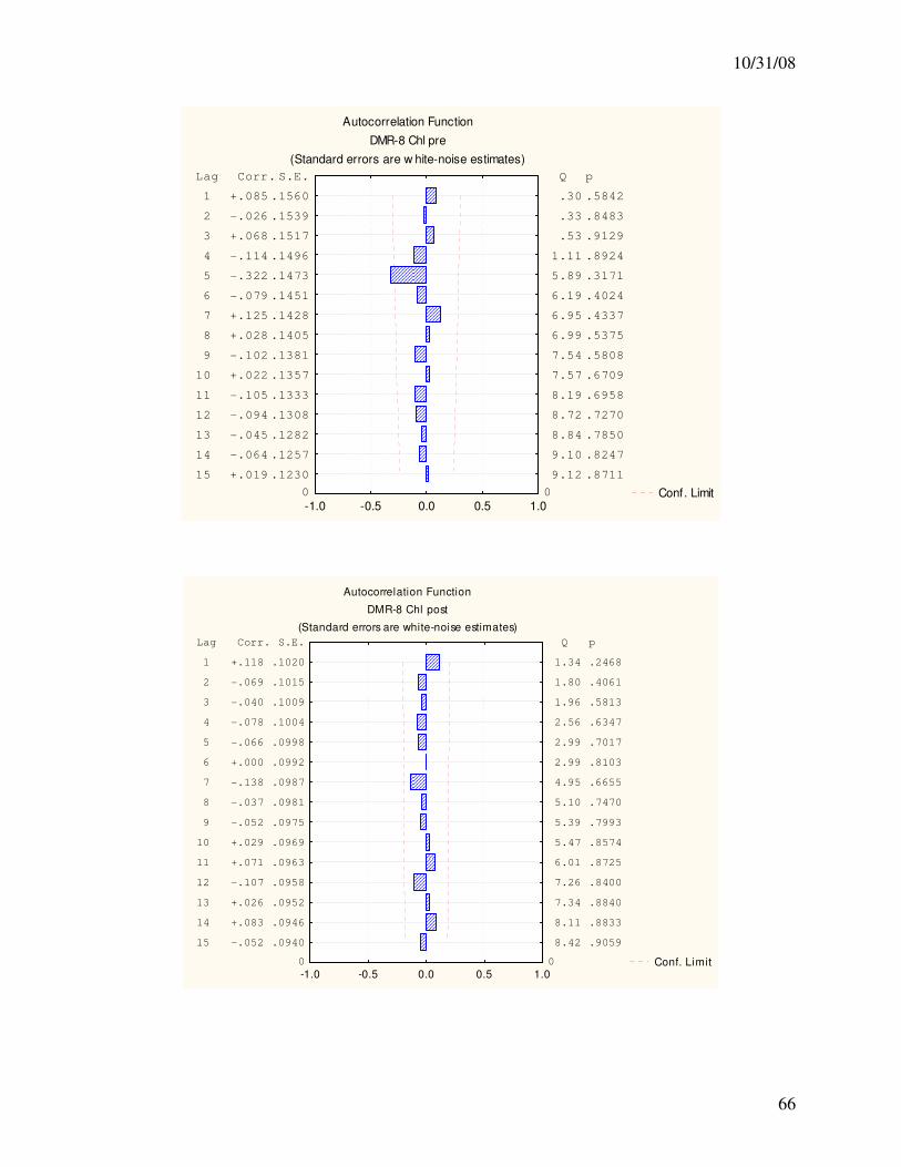
10/31/08
66
Autocorrelation Function
DMR-8 Chl pre
(Standard errors are w hite-noise estimates)
Conf. Limit-1.0 -0.5 0.0 0.5 1.00
15 +.019 .1230
14 -.064 .1257
13 -.045 .1282
12 -.094 .1308
11 -.105 .1333
10 +.022 .1357
9 -.102 .1381
8 +.028 .1405
7 +.125 .1428
6 -.079 .1451
5 -.322 .1473
4 -.114 .1496
3 +.068 .1517
2 -.026 .1539
1 +.085 .1560
Lag Corr. S.E.
0
9.12 .8711
9.10 .8247
8.84 .7850
8.72 .7270
8.19 .6958
7.57 .6709
7.54 .5808
6.99 .5375
6.95 .4337
6.19 .4024
5.89 .3171
1.11 .8924
.53 .9129
.33 .8483
.30 .5842
Q p
Autocorrelation Function
DMR-8 Chl post
(Standard errors are white-noise estimates)
Conf. Limit-1.0 -0.5 0.0 0.5 1.00
15 -.052 .0940
14 +.083 .0946
13 +.026 .0952
12 -.107 .0958
11 +.071 .0963
10 +.029 .0969
9 -.052 .0975
8 -.037 .0981
7 -.138 .0987
6 +.000 .0992
5 -.066 .0998
4 -.078 .1004
3 -.040 .1009
2 -.069 .1015
1 +.118 .1020
Lag Corr. S.E.
0
8.42 .9059
8.11 .8833
7.34 .8840
7.26 .8400
6.01 .8725
5.47 .8574
5.39 .7993
5.10 .7470
4.95 .6655
2.99 .8103
2.99 .7017
2.56 .6347
1.96 .5813
1.80 .4061
1.34 .2468
Q p
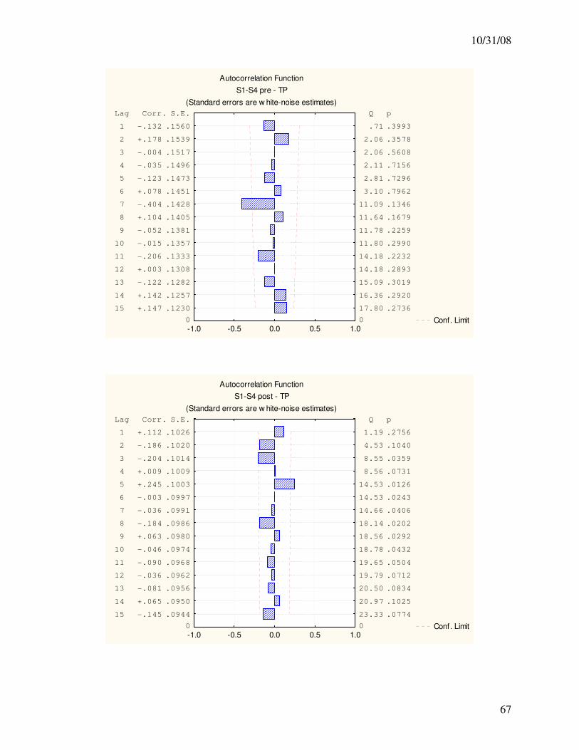
10/31/08
67
Autocorrelation Function
S1-S4 pre - TP
(Standard errors are w hite-noise estimates)
Conf. Limit-1.0 -0.5 0.0 0.5 1.00
15 +.147 .1230
14 +.142 .1257
13 -.122 .1282
12 +.003 .1308
11 -.206 .1333
10 -.015 .1357
9 -.052 .1381
8 +.104 .1405
7 -.404 .1428
6 +.078 .1451
5 -.123 .1473
4 -.035 .1496
3 -.004 .1517
2 +.178 .1539
1 -.132 .1560
Lag Corr. S.E.
0
17.80 .2736
16.36 .2920
15.09 .3019
14.18 .2893
14.18 .2232
11.80 .2990
11.78 .2259
11.64 .1679
11.09 .1346
3.10 .7962
2.81 .7296
2.11 .7156
2.06 .5608
2.06 .3578
.71 .3993
Q p
Autocorrelation Function
S1-S4 post - TP
(Standard errors are w hite-noise estimates)
Conf. Limit-1.0 -0.5 0.0 0.5 1.00
15 -.145 .0944
14 +.065 .0950
13 -.081 .0956
12 -.036 .0962
11 -.090 .0968
10 -.046 .0974
9 +.063 .0980
8 -.184 .0986
7 -.036 .0991
6 -.003 .0997
5 +.245 .1003
4 +.009 .1009
3 -.204 .1014
2 -.186 .1020
1 +.112 .1026
Lag Corr. S.E.
0
23.33 .0774
20.97 .1025
20.50 .0834
19.79 .0712
19.65 .0504
18.78 .0432
18.56 .0292
18.14 .0202
14.66 .0406
14.53 .0243
14.53 .0126
8.56 .0731
8.55 .0359
4.53 .1040
1.19 .2756
Q p
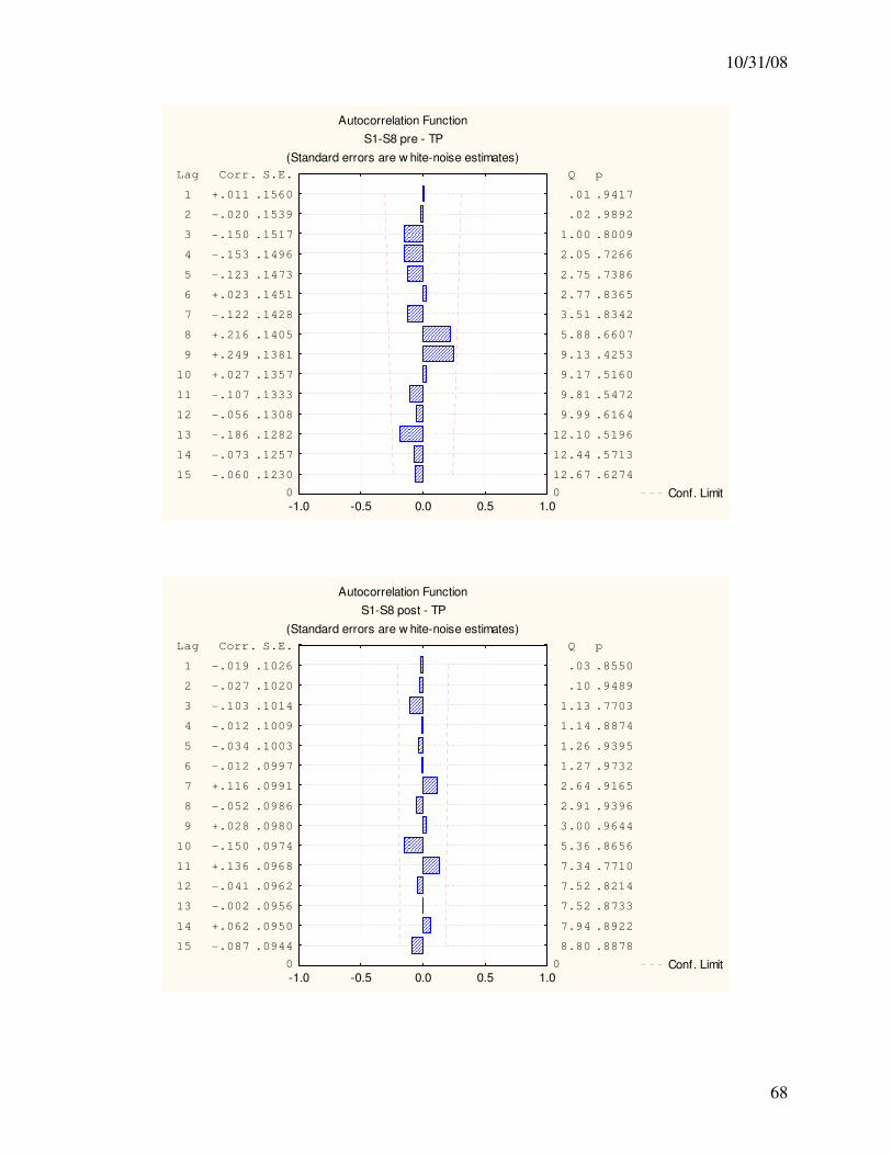
10/31/08
68
Autocorrelation Function
S1-S8 pre - TP
(Standard errors are w hite-noise estimates)
Conf. Limit-1.0 -0.5 0.0 0.5 1.00
15 -.060 .1230
14 -.073 .1257
13 -.186 .1282
12 -.056 .1308
11 -.107 .1333
10 +.027 .1357
9 +.249 .1381
8 +.216 .1405
7 -.122 .1428
6 +.023 .1451
5 -.123 .1473
4 -.153 .1496
3 -.150 .1517
2 -.020 .1539
1 +.011 .1560
Lag Corr. S.E.
0
12.67 .6274
12.44 .5713
12.10 .5196
9.99 .6164
9.81 .5472
9.17 .5160
9.13 .4253
5.88 .6607
3.51 .8342
2.77 .8365
2.75 .7386
2.05 .7266
1.00 .8009
.02 .9892
.01 .9417
Q p
Autocorrelation Function
S1-S8 post - TP
(Standard errors are w hite-noise estimates)
Conf. Limit-1.0 -0.5 0.0 0.5 1.00
15 -.087 .0944
14 +.062 .0950
13 -.002 .0956
12 -.041 .0962
11 +.136 .0968
10 -.150 .0974
9 +.028 .0980
8 -.052 .0986
7 +.116 .0991
6 -.012 .0997
5 -.034 .1003
4 -.012 .1009
3 -.103 .1014
2 -.027 .1020
1 -.019 .1026
Lag Corr. S.E.
0
8.80 .8878
7.94 .8922
7.52 .8733
7.52 .8214
7.34 .7710
5.36 .8656
3.00 .9644
2.91 .9396
2.64 .9165
1.27 .9732
1.26 .9395
1.14 .8874
1.13 .7703
.10 .9489
.03 .8550
Q p
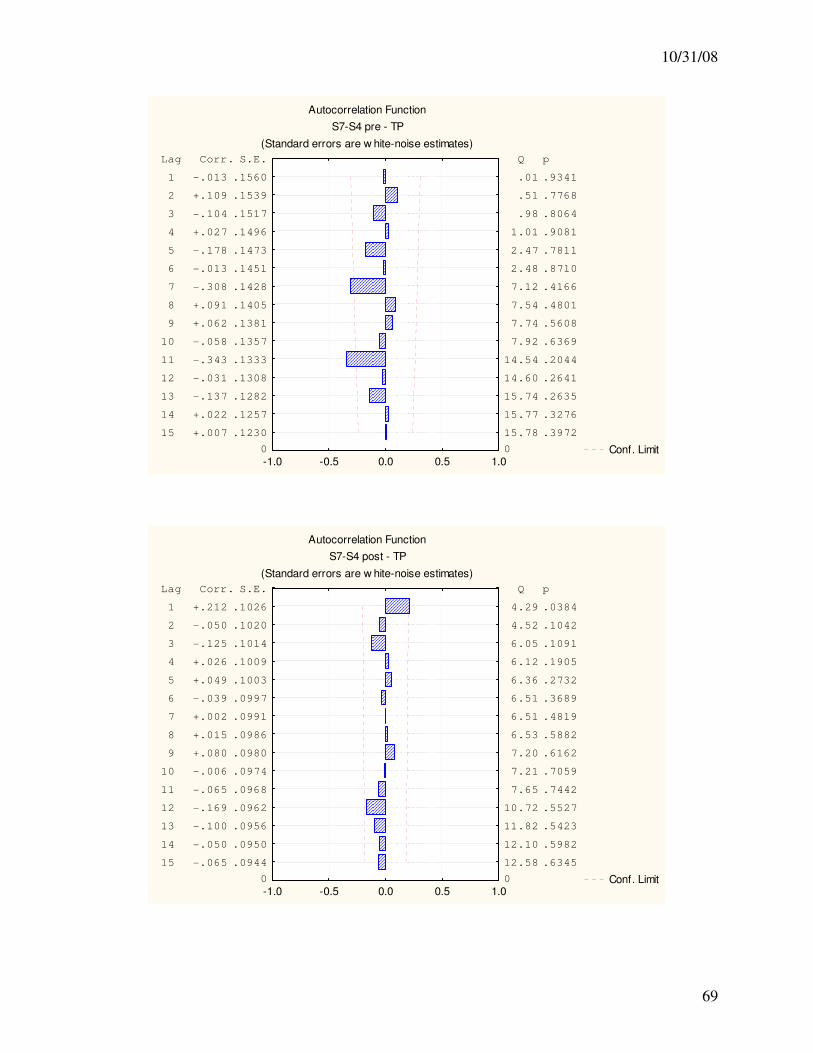
10/31/08
69
Autocorrelation Function
S7-S4 pre - TP
(Standard errors are w hite-noise estimates)
Conf. Limit-1.0 -0.5 0.0 0.5 1.00
15 +.007 .1230
14 +.022 .1257
13 -.137 .1282
12 -.031 .1308
11 -.343 .1333
10 -.058 .1357
9 +.062 .1381
8 +.091 .1405
7 -.308 .1428
6 -.013 .1451
5 -.178 .1473
4 +.027 .1496
3 -.104 .1517
2 +.109 .1539
1 -.013 .1560
Lag Corr. S.E.
0
15.78 .3972
15.77 .3276
15.74 .2635
14.60 .2641
14.54 .2044
7.92 .6369
7.74 .5608
7.54 .4801
7.12 .4166
2.48 .8710
2.47 .7811
1.01 .9081
.98 .8064
.51 .7768
.01 .9341
Q p
Autocorrelation Function
S7-S4 post - TP
(Standard errors are w hite-noise estimates)
Conf. Limit-1.0 -0.5 0.0 0.5 1.00
15 -.065 .0944
14 -.050 .0950
13 -.100 .0956
12 -.169 .0962
11 -.065 .0968
10 -.006 .0974
9 +.080 .0980
8 +.015 .0986
7 +.002 .0991
6 -.039 .0997
5 +.049 .1003
4 +.026 .1009
3 -.125 .1014
2 -.050 .1020
1 +.212 .1026
Lag Corr. S.E.
0
12.58 .6345
12.10 .5982
11.82 .5423
10.72 .5527
7.65 .7442
7.21 .7059
7.20 .6162
6.53 .5882
6.51 .4819
6.51 .3689
6.36 .2732
6.12 .1905
6.05 .1091
4.52 .1042
4.29 .0384
Q p
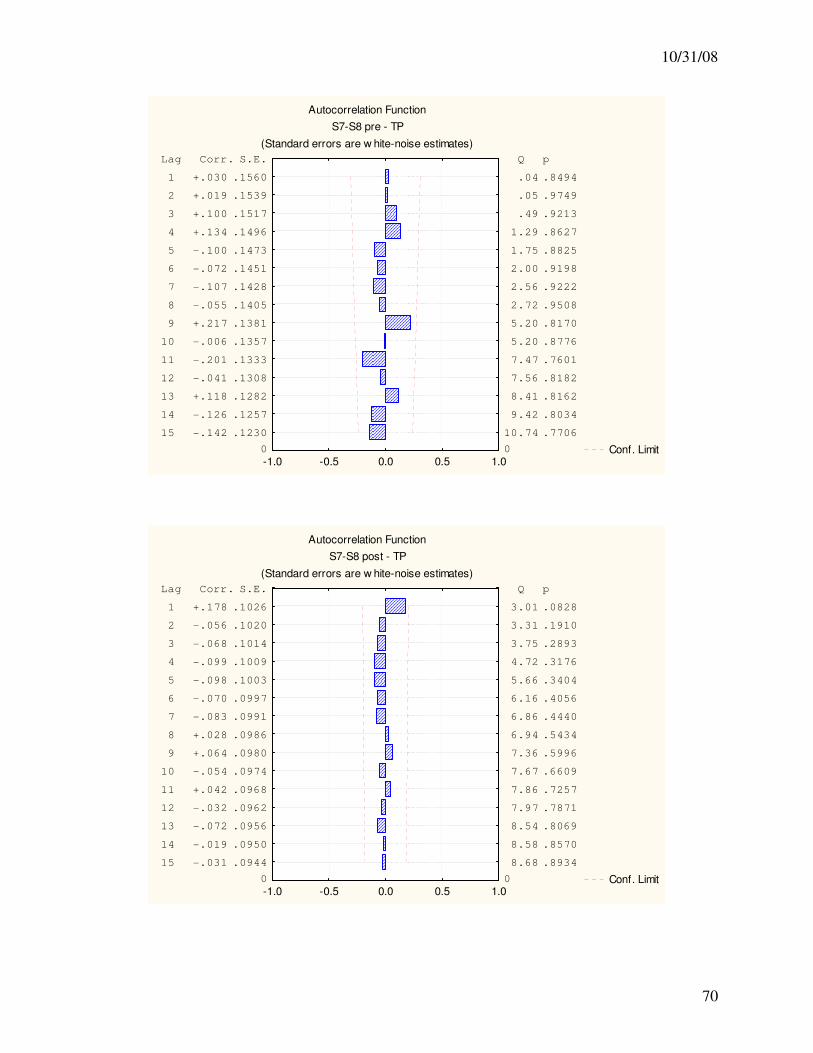
10/31/08
70
Autocorrelation Function
S7-S8 pre - TP
(Standard errors are w hite-noise estimates)
Conf. Limit-1.0 -0.5 0.0 0.5 1.00
15 -.142 .1230
14 -.126 .1257
13 +.118 .1282
12 -.041 .1308
11 -.201 .1333
10 -.006 .1357
9 +.217 .1381
8 -.055 .1405
7 -.107 .1428
6 -.072 .1451
5 -.100 .1473
4 +.134 .1496
3 +.100 .1517
2 +.019 .1539
1 +.030 .1560
Lag Corr. S.E.
0
10.74 .7706
9.42 .8034
8.41 .8162
7.56 .8182
7.47 .7601
5.20 .8776
5.20 .8170
2.72 .9508
2.56 .9222
2.00 .9198
1.75 .8825
1.29 .8627
.49 .9213
.05 .9749
.04 .8494
Q p
Autocorrelation Function
S7-S8 post - TP
(Standard errors are w hite-noise estimates)
Conf. Limit-1.0 -0.5 0.0 0.5 1.00
15 -.031 .0944
14 -.019 .0950
13 -.072 .0956
12 -.032 .0962
11 +.042 .0968
10 -.054 .0974
9 +.064 .0980
8 +.028 .0986
7 -.083 .0991
6 -.070 .0997
5 -.098 .1003
4 -.099 .1009
3 -.068 .1014
2 -.056 .1020
1 +.178 .1026
Lag Corr. S.E.
0
8.68 .8934
8.58 .8570
8.54 .8069
7.97 .7871
7.86 .7257
7.67 .6609
7.36 .5996
6.94 .5434
6.86 .4440
6.16 .4056
5.66 .3404
4.72 .3176
3.75 .2893
3.31 .1910
3.01 .0828
Q p
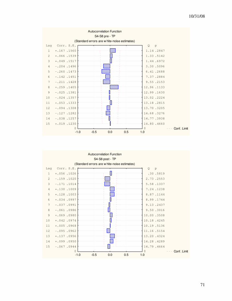
10/31/08
71
Autocorrelation Function
S4-S8 pre - TP
(Standard errors are w hite-noise estimates)
Conf. Limit-1.0 -0.5 0.0 0.5 1.00
15 +.019 .1230
14 -.038 .1257
13 -.127 .1282
12 -.094 .1308
11 +.053 .1333
10 -.024 .1357
9 -.025 .1381
8 +.259 .1405
7 -.211 .1428
6 -.142 .1451
5 -.260 .1473
4 -.204 .1496
3 +.049 .1517
2 +.066 .1539
1 +.167 .1560
Lag Corr. S.E.
0
14.80 .4660
14.77 .3938
14.68 .3276
13.70 .3205
13.18 .2815
13.02 .2224
12.99 .1630
12.96 .1133
9.55 .2153
7.37 .2884
6.41 .2688
3.30 .5096
1.44 .6972
1.33 .5142
1.14 .2847
Q p
Autocorrelation Function
S4-S8 post - TP
(Standard errors are w hite-noise estimates)
Conf. Limit-1.0 -0.5 0.0 0.5 1.00
15 -.067 .0944
14 +.099 .0950
13 +.137 .0956
12 -.095 .0962
11 +.005 .0968
10 +.042 .0974
9 +.069 .0980
8 -.061 .0986
7 -.037 .0991
6 +.034 .0997
5 +.128 .1003
4 +.130 .1009
3 -.171 .1014
2 -.159 .1020
1 +.056 .1026
Lag Corr. S.E.
0
14.79 .4664
14.28 .4289
13.20 .4324
11.16 .5154
10.19 .5136
10.18 .4245
10.00 .3508
9.50 .3016
9.13 .2437
8.99 .1744
8.87 .1144
7.24 .1238
5.58 .1337
2.73 .2553
.30 .5819
Q p
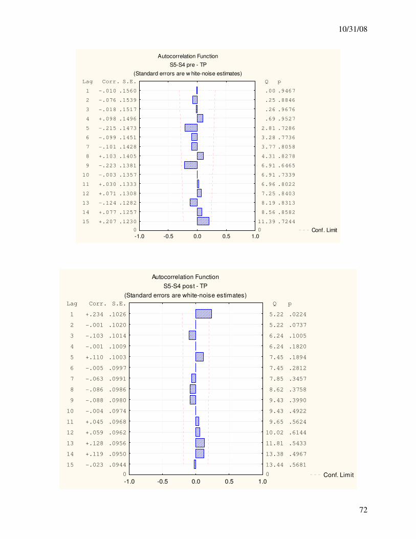
10/31/08
72
Autocorrelation Function
S5-S4 pre - TP
(Standard errors are w hite-noise estimates)
Conf. Limit-1.0 -0.5 0.0 0.5 1.00
15 +.207 .1230
14 +.077 .1257
13 -.124 .1282
12 +.071 .1308
11 +.030 .1333
10 -.003 .1357
9 -.223 .1381
8 +.103 .1405
7 -.101 .1428
6 -.099 .1451
5 -.215 .1473
4 +.098 .1496
3 -.018 .1517
2 -.076 .1539
1 -.010 .1560
Lag Corr. S.E.
0
11.39 .7244
8.56 .8582
8.19 .8313
7.25 .8403
6.96 .8022
6.91 .7339
6.91 .6465
4.31 .8278
3.77 .8058
3.28 .7736
2.81 .7286
.69 .9527
.26 .9676
.25 .8846
.00 .9467
Q p
Autocorrelation Function
S5-S4 post - TP
(Standard errors are white-noise estimates)
Conf. Limit-1.0 -0.5 0.0 0.5 1.0
0
15 -.023 .0944
14 +.119 .0950
13 +.128 .0956
12 +.059 .0962
11 +.045 .0968
10 -.004 .0974
9 -.088 .0980
8 -.086 .0986
7 -.063 .0991
6 -.005 .0997
5 +.110 .1003
4 -.001 .1009
3 -.103 .1014
2 -.001 .1020
1 +.234 .1026
Lag Corr. S.E.
0
13.44 .5681
13.38 .4967
11.81 .5433
10.02 .6144
9.65 .5624
9.43 .4922
9.43 .3990
8.62 .3758
7.85 .3457
7.45 .2812
7.45 .1894
6.24 .1820
6.24 .1005
5.22 .0737
5.22 .0224
Q p
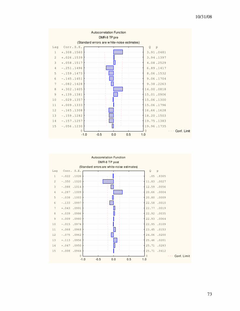
10/31/08
73
Autocorrelation Function
DMR-8 TP pre
(Standard errors are w hite-noise estimates)
Conf. Limit-1.0 -0.5 0.0 0.5 1.00
15 -.056 .1230
14 -.157 .1257
13 -.159 .1282
12 -.165 .1308
11 +.009 .1333
10 -.029 .1357
9 +.139 .1381
8 +.302 .1405
7 -.082 .1428
6 -.145 .1451
5 -.159 .1473
4 -.251 .1496
3 +.058 .1517
2 +.026 .1539
1 +.308 .1560
Lag Corr. S.E.
0
19.96 .1735
19.75 .1383
18.20 .1503
16.66 .1628
15.06 .1796
15.06 .1300
15.01 .0906
14.00 .0818
9.38 .2263
9.06 .1704
8.06 .1532
6.89 .1417
4.08 .2529
3.94 .1397
3.91 .0481
Q p
Autocorrelation Function
DMR-8 TP post
(Standard errors are white-noise estimates)
Conf. Limit-1.0 -0.5 0.0 0.5 1.0
0
15 +.008 .0944
14 +.047 .0950
13 +.113 .0956
12 -.075 .0962
11 +.068 .0968
10 -.015 .0974
9 +.009 .0980
8 +.039 .0986
7 +.043 .0991
6 -.133 .0997
5 -.038 .1003
4 +.287 .1009
3 -.088 .1014
2 -.350 .1020
1 -.022 .1026
Lag Corr. S.E.
0
25.71 .0412
25.71 .0283
25.46 .0201
24.06 .0200
23.45 .0153
22.95 .0109
22.93 .0064
22.92 .0035
22.77 .0019
22.58 .0010
20.80 .0009
20.66 .0004
12.59 .0056
11.83 .0027
.05 .8305
Q p
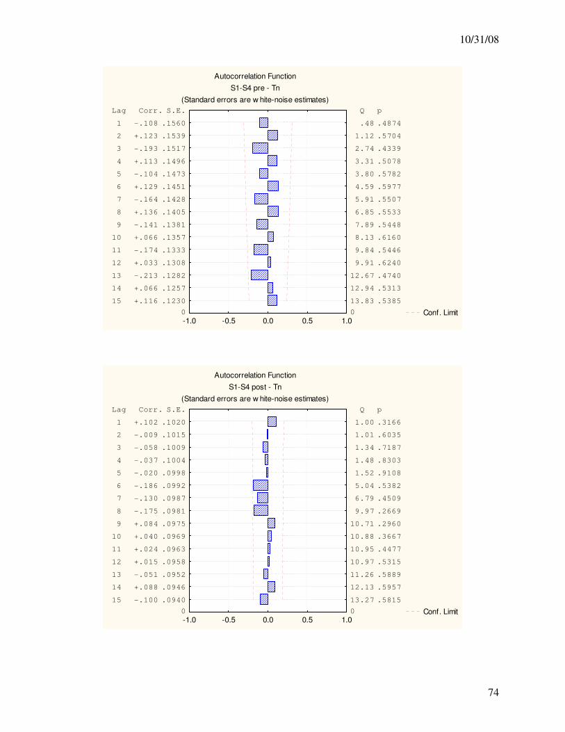
10/31/08
74
Autocorrelation Function
S1-S4 pre - Tn
(Standard errors are w hite-noise estimates)
Conf. Limit-1.0 -0.5 0.0 0.5 1.00
15 +.116 .1230
14 +.066 .1257
13 -.213 .1282
12 +.033 .1308
11 -.174 .1333
10 +.066 .1357
9 -.141 .1381
8 +.136 .1405
7 -.164 .1428
6 +.129 .1451
5 -.104 .1473
4 +.113 .1496
3 -.193 .1517
2 +.123 .1539
1 -.108 .1560
Lag Corr. S.E.
0
13.83 .5385
12.94 .5313
12.67 .4740
9.91 .6240
9.84 .5446
8.13 .6160
7.89 .5448
6.85 .5533
5.91 .5507
4.59 .5977
3.80 .5782
3.31 .5078
2.74 .4339
1.12 .5704
.48 .4874
Q p
Autocorrelation Function
S1-S4 post - Tn
(Standard errors are w hite-noise estimates)
Conf. Limit-1.0 -0.5 0.0 0.5 1.00
15 -.100 .0940
14 +.088 .0946
13 -.051 .0952
12 +.015 .0958
11 +.024 .0963
10 +.040 .0969
9 +.084 .0975
8 -.175 .0981
7 -.130 .0987
6 -.186 .0992
5 -.020 .0998
4 -.037 .1004
3 -.058 .1009
2 -.009 .1015
1 +.102 .1020
Lag Corr. S.E.
0
13.27 .5815
12.13 .5957
11.26 .5889
10.97 .5315
10.95 .4477
10.88 .3667
10.71 .2960
9.97 .2669
6.79 .4509
5.04 .5382
1.52 .9108
1.48 .8303
1.34 .7187
1.01 .6035
1.00 .3166
Q p
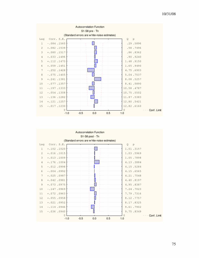
10/31/08
75
Autocorrelation Function
S1-S8 pre - Tn
(Standard errors are w hite-noise estimates)
Conf. Limit-1.0 -0.5 0.0 0.5 1.00
15 -.017 .1230
14 +.121 .1257
13 -.136 .1282
12 -.054 .1308
11 -.197 .1333
10 -.077 .1357
9 +.241 .1381
8 -.075 .1405
7 -.252 .1428
6 +.059 .1451
5 +.112 .1473
4 +.033 .1496
3 +.080 .1517
2 +.082 .1539
1 -.084 .1560
Lag Corr. S.E.
0
12.82 .6160
12.80 .5421
11.87 .5383
10.75 .5502
10.58 .4787
8.41 .5890
8.08 .5257
5.04 .7537
4.75 .6903
1.65 .9490
1.48 .9150
.90 .9240
.86 .8362
.58 .7496
.29 .5896
Q p
Autocorrelation Function
S1-S8 post - Tn
(Standard errors are w hite-noise estimates)
Conf. Limit-1.0 -0.5 0.0 0.5 1.00
15 -.036 .0940
14 -.114 .0946
13 +.021 .0952
12 +.055 .0958
11 +.072 .0963
10 -.147 .0969
9 +.073 .0975
8 +.042 .0981
7 +.025 .0987
6 -.004 .0992
5 -.012 .0998
4 +.176 .1004
3 +.013 .1009
2 +.016 .1015
1 +.102 .1020
Lag Corr. S.E.
0
9.75 .8349
9.61 .7902
8.17 .8325
8.12 .7757
7.79 .7316
7.24 .7023
4.95 .8387
4.40 .8197
4.21 .7548
4.15 .6565
4.15 .5284
4.13 .3884
1.05 .7898
1.03 .5969
1.01 .3157
Q p
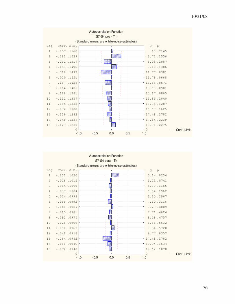
10/31/08
76
Autocorrelation Function
S7-S4 pre - Tn
(Standard errors are w hite-noise estimates)
Conf. Limit-1.0 -0.5 0.0 0.5 1.00
15 +.127 .1230
14 -.049 .1257
13 -.116 .1282
12 -.074 .1308
11 -.094 .1333
10 -.112 .1357
9 -.168 .1381
8 +.014 .1405
7 -.197 .1428
6 -.020 .1451
5 -.318 .1473
4 +.153 .1496
3 -.232 .1517
2 +.291 .1539
1 +.057 .1560
Lag Corr. S.E.
0
18.71 .2275
17.64 .2239
17.48 .1782
16.67 .1625
16.35 .1287
15.85 .1040
15.17 .0865
13.69 .0901
13.68 .0571
11.79 .0668
11.77 .0381
7.10 .1306
6.06 .1087
3.72 .1556
.13 .7145
Q p
Autocorrelation Function
S7-S4 post - Tn
(Standard errors are w hite-noise estimates)
Conf. Limit-1.0 -0.5 0.0 0.5 1.00
15 -.072 .0940
14 -.118 .0946
13 -.264 .0952
12 -.046 .0958
11 +.090 .0963
10 -.028 .0969
9 -.092 .0975
8 -.065 .0981
7 +.041 .0987
6 -.099 .0992
5 -.024 .0998
4 -.037 .1004
3 -.084 .1009
2 -.026 .1015
1 +.231 .1020
Lag Corr. S.E.
0
19.62 .1870
19.04 .1634
17.48 .1782
9.77 .6357
9.54 .5720
8.68 .5632
8.59 .4757
7.71 .4624
7.27 .4009
7.10 .3116
6.10 .2967
6.04 .1962
5.90 .1165
5.21 .0741
5.14 .0234
Q p
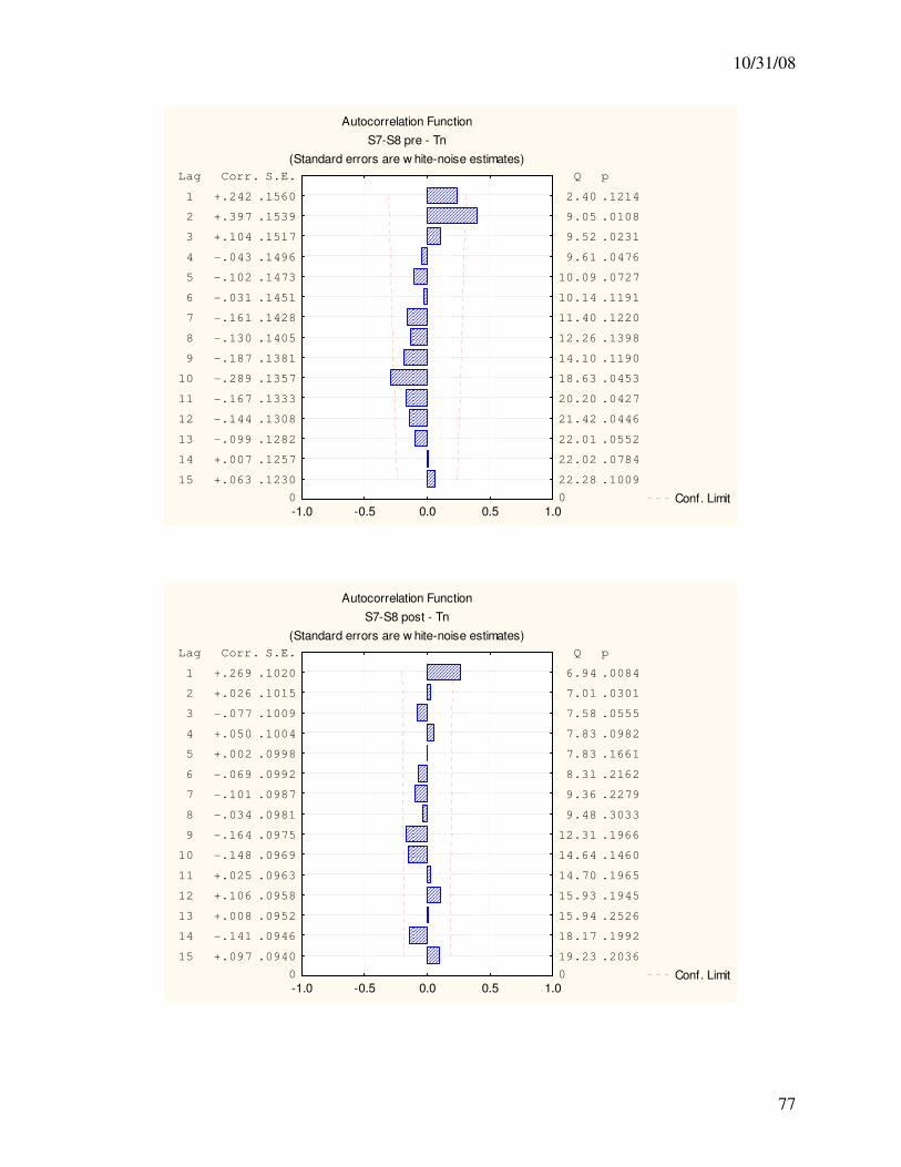
10/31/08
77
Autocorrelation Function
S7-S8 pre - Tn
(Standard errors are w hite-noise estimates)
Conf. Limit-1.0 -0.5 0.0 0.5 1.00
15 +.063 .1230
14 +.007 .1257
13 -.099 .1282
12 -.144 .1308
11 -.167 .1333
10 -.289 .1357
9 -.187 .1381
8 -.130 .1405
7 -.161 .1428
6 -.031 .1451
5 -.102 .1473
4 -.043 .1496
3 +.104 .1517
2 +.397 .1539
1 +.242 .1560
Lag Corr. S.E.
0
22.28 .1009
22.02 .0784
22.01 .0552
21.42 .0446
20.20 .0427
18.63 .0453
14.10 .1190
12.26 .1398
11.40 .1220
10.14 .1191
10.09 .0727
9.61 .0476
9.52 .0231
9.05 .0108
2.40 .1214
Q p
Autocorrelation Function
S7-S8 post - Tn
(Standard errors are w hite-noise estimates)
Conf. Limit-1.0 -0.5 0.0 0.5 1.00
15 +.097 .0940
14 -.141 .0946
13 +.008 .0952
12 +.106 .0958
11 +.025 .0963
10 -.148 .0969
9 -.164 .0975
8 -.034 .0981
7 -.101 .0987
6 -.069 .0992
5 +.002 .0998
4 +.050 .1004
3 -.077 .1009
2 +.026 .1015
1 +.269 .1020
Lag Corr. S.E.
0
19.23 .2036
18.17 .1992
15.94 .2526
15.93 .1945
14.70 .1965
14.64 .1460
12.31 .1966
9.48 .3033
9.36 .2279
8.31 .2162
7.83 .1661
7.83 .0982
7.58 .0555
7.01 .0301
6.94 .0084
Q p
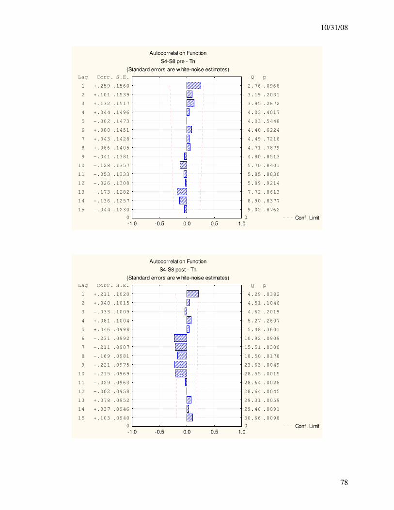
10/31/08
78
Autocorrelation Function
S4-S8 pre - Tn
(Standard errors are w hite-noise estimates)
Conf. Limit-1.0 -0.5 0.0 0.5 1.00
15 -.044 .1230
14 -.136 .1257
13 -.173 .1282
12 -.026 .1308
11 -.053 .1333
10 -.128 .1357
9 -.041 .1381
8 +.066 .1405
7 +.043 .1428
6 +.088 .1451
5 -.002 .1473
4 +.044 .1496
3 +.132 .1517
2 +.101 .1539
1 +.259 .1560
Lag Corr. S.E.
0
9.02 .8762
8.90 .8377
7.72 .8613
5.89 .9214
5.85 .8830
5.70 .8401
4.80 .8513
4.71 .7879
4.49 .7216
4.40 .6224
4.03 .5448
4.03 .4017
3.95 .2672
3.19 .2031
2.76 .0968
Q p
Autocorrelation Function
S4-S8 post - Tn
(Standard errors are w hite-noise estimates)
Conf. Limit-1.0 -0.5 0.0 0.5 1.00
15 +.103 .0940
14 +.037 .0946
13 +.078 .0952
12 -.002 .0958
11 -.029 .0963
10 -.215 .0969
9 -.221 .0975
8 -.169 .0981
7 -.211 .0987
6 -.231 .0992
5 +.046 .0998
4 +.081 .1004
3 -.033 .1009
2 +.048 .1015
1 +.211 .1020
Lag Corr. S.E.
0
30.66 .0098
29.46 .0091
29.31 .0059
28.64 .0045
28.64 .0026
28.55 .0015
23.63 .0049
18.50 .0178
15.51 .0300
10.92 .0909
5.48 .3601
5.27 .2607
4.62 .2019
4.51 .1046
4.29 .0382
Q p
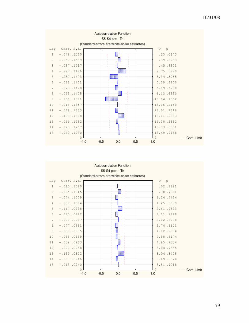
10/31/08
79
Autocorrelation Function
S5-S4 pre - Tn
(Standard errors are w hite-noise estimates)
Conf. Limit-1.0 -0.5 0.0 0.5 1.00
15 +.049 .1230
14 +.023 .1257
13 -.055 .1282
12 +.166 .1308
11 -.079 .1333
10 -.016 .1357
9 -.366 .1381
8 +.093 .1405
7 -.078 .1428
6 -.031 .1451
5 -.237 .1473
4 +.227 .1496
3 -.037 .1517
2 +.057 .1539
1 -.078 .1560
Lag Corr. S.E.
0
15.49 .4168
15.33 .3561
15.30 .2892
15.11 .2353
13.51 .2616
13.16 .2150
13.14 .1562
6.13 .6330
5.69 .5768
5.39 .4950
5.34 .3755
2.75 .5999
.45 .9301
.39 .8233
.25 .6173
Q p
Autocorrelation Function
S5-S4 post - Tn
(Standard errors are w hite-noise estimates)
Conf. Limit-1.0 -0.5 0.0 0.5 1.00
15 +.013 .0940
14 -.063 .0946
13 +.165 .0952
12 -.029 .0958
11 +.059 .0963
10 -.066 .0969
9 -.060 .0975
8 -.077 .0981
7 +.009 .0987
6 -.070 .0992
5 +.117 .0998
4 -.007 .1004
3 -.074 .1009
2 +.084 .1015
1 -.015 .1020
Lag Corr. S.E.
0
8.51 .9018
8.49 .8624
8.04 .8408
5.04 .9565
4.95 .9334
4.58 .9174
4.12 .9034
3.74 .8801
3.12 .8738
3.11 .7948
2.61 .7593
1.25 .8699
1.24 .7424
.70 .7031
.02 .8821
Q p
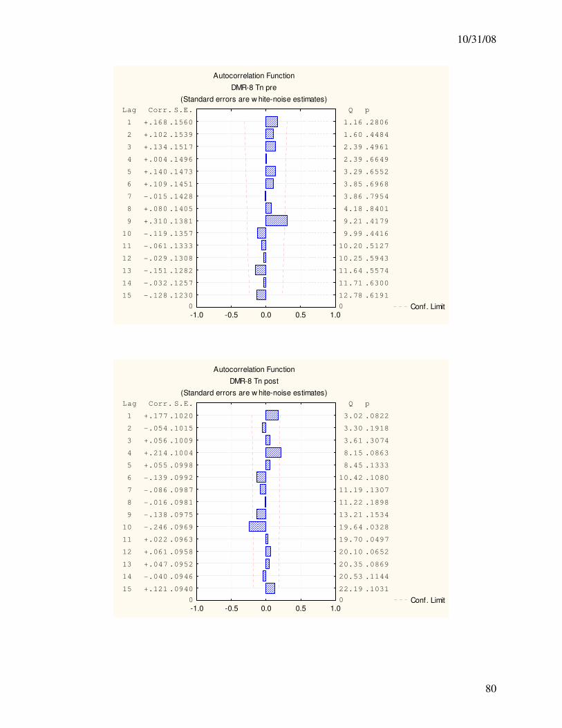
10/31/08
80
Autocorrelation Function
DMR-8 Tn pre
(Standard errors are w hite-noise estimates)
Conf. Limit-1.0 -0.5 0.0 0.5 1.00
15 -.128 .1230
14 -.032 .1257
13 -.151 .1282
12 -.029 .1308
11 -.061 .1333
10 -.119 .1357
9 +.310 .1381
8 +.080 .1405
7 -.015 .1428
6 +.109 .1451
5 +.140 .1473
4 +.004 .1496
3 +.134 .1517
2 +.102 .1539
1 +.168 .1560
Lag Corr. S.E.
0
12.78 .6191
11.71 .6300
11.64 .5574
10.25 .5943
10.20 .5127
9.99 .4416
9.21 .4179
4.18 .8401
3.86 .7954
3.85 .6968
3.29 .6552
2.39 .6649
2.39 .4961
1.60 .4484
1.16 .2806
Q p
Autocorrelation Function
DMR-8 Tn post
(Standard errors are w hite-noise estimates)
Conf. Limit-1.0 -0.5 0.0 0.5 1.00
15 +.121 .0940
14 -.040 .0946
13 +.047 .0952
12 +.061 .0958
11 +.022 .0963
10 -.246 .0969
9 -.138 .0975
8 -.016 .0981
7 -.086 .0987
6 -.139 .0992
5 +.055 .0998
4 +.214 .1004
3 +.056 .1009
2 -.054 .1015
1 +.177 .1020
Lag Corr. S.E.
0
22.19 .1031
20.53 .1144
20.35 .0869
20.10 .0652
19.70 .0497
19.64 .0328
13.21 .1534
11.22 .1898
11.19 .1307
10.42 .1080
8.45 .1333
8.15 .0863
3.61 .3074
3.30 .1918
3.02 .0822
Q p

10/31/08
81
Appendix 3 - Additivity
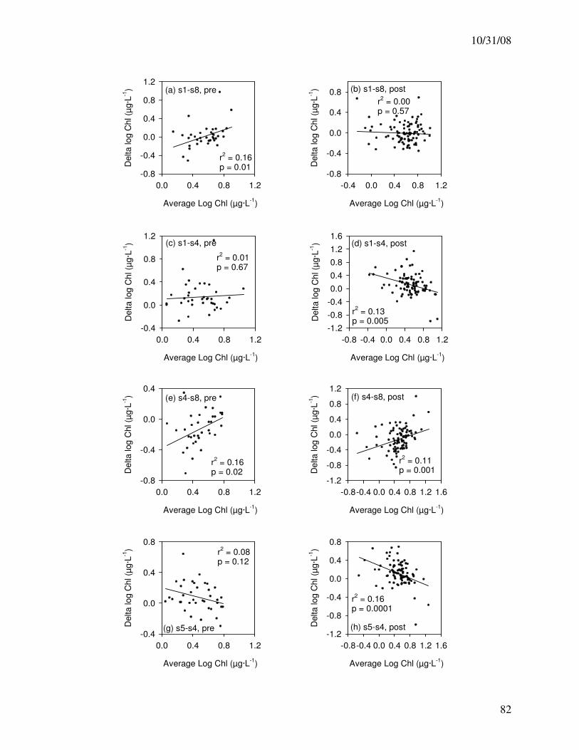
10/31/08
82
Average Log Chl (µg·L-1
)
0.0 0.4 0.8 1.2
Delta log C
hl (µ
g·L
-1)
-0.8
-0.4
0.0
0.4
0.8
1.2(a) s1-s8, pre
r2 = 0.16
p = 0.01
Average Log Chl (µg·L-1
)
-0.4 0.0 0.4 0.8 1.2
Delta log C
hl (µ
g·L
-1)
-0.8
-0.4
0.0
0.4
0.8r2 = 0.00
p = 0.57
(b) s1-s8, post
Average Log Chl (µg·L-1
)
0.0 0.4 0.8 1.2
Delta log C
hl (µ
g·L
-1)
-0.8
-0.4
0.0
0.4
(c) s1-s4, pre
r2 = 0.01
p = 0.67
Average Log Chl (µg·L-1
)
-0.8-0.4 0.0 0.4 0.8 1.2 1.6
Delta log C
hl (µ
g·L
-1)
-1.2
-0.8
-0.4
0.0
0.4
0.8
1.2
(d) s1-s4, post
r2 = 0.13
p = 0.005
Average Log Chl (µg·L-1
)
0.0 0.4 0.8 1.2
Delta log C
hl (µ
g·L
-1)
-0.4
0.0
0.4
0.8
Average Log Chl (µg·L-1
)
-0.8-0.4 0.0 0.4 0.8 1.2 1.6
Delta log C
hl (µ
g·L
-1)
-1.2
-0.8
-0.4
0.0
0.4
0.8
(e) s4-s8, pre (f) s4-s8, post
(g) s5-s4, pre (h) s5-s4, post
r2 = 0.16
p = 0.02
r2 = 0.11
p = 0.001
Average Log Chl (µg·L-1
)
0.0 0.4 0.8 1.2
Delta log C
hl (µ
g·L
-1)
-0.4
0.0
0.4
0.8
1.2
Average Log Chl (µg·L-1
)
-0.8 -0.4 0.0 0.4 0.8 1.2
Delta log C
hl (µ
g·L
-1)
-1.2
-0.8
-0.4
0.0
0.4
0.8
1.2
1.6
r2 = 0.08
p = 0.12
r2 = 0.16
p = 0.0001
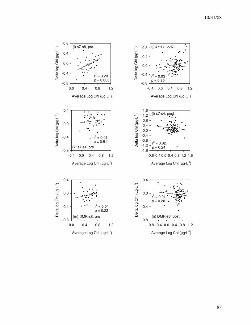
10/31/08
83
Average Log Chl (µg·L-1
)
0.0 0.4 0.8 1.2
De
lta lo
g C
hl (µ
g·L
-1)
-0.8
-0.4
0.0
0.4
0.8(i) s7-s8, pre
r2 = 0.20
p = 0.005
Average Log Chl (µg·L-1
)
-0.4 0.0 0.4 0.8 1.2
De
lta lo
g C
hl (µ
g·L
-1)
-0.8
-0.4
0.0
0.4
0.8
r2 = 0.03
p = 0.30
(j) s7-s8, post
(k) s7-s4, pre
r2 = 0.01
p = 0.51
(l) s7-s4, post
r2 = 0.02
p = 0.24
Average Log Chl (µg·L-1
)
-0.4 0.0 0.4 0.8 1.2
De
lta
log
Ch
l (µ
g·L
-1)
-0.8
-0.4
0.0
0.4
Average Log Chl (µg·L-1
)
-0.8-0.4 0.0 0.4 0.8 1.2 1.6
De
lta
log
Ch
l (µ
g·L
-1)
-1.6
-1.2
-0.8
-0.4
0.0
0.4
0.8
1.2
1.6
Average Log Chl (µg·L-1
)
0.0 0.4 0.8 1.2
De
lta lo
g C
hl (µ
g·L
-1)
-0.8
-0.4
0.0
0.4
Average Log Chl (µg·L-1
)
-0.8 -0.4 0.0 0.4 0.8 1.2
De
lta lo
g C
hl (µ
g·L
-1)
-0.8
-0.4
0.0
0.4
(m) DMR-s8, pre (n) DMR-s8, post
r2 = 0.04
p = 0.22
r2 = 0.01
p = 0.28
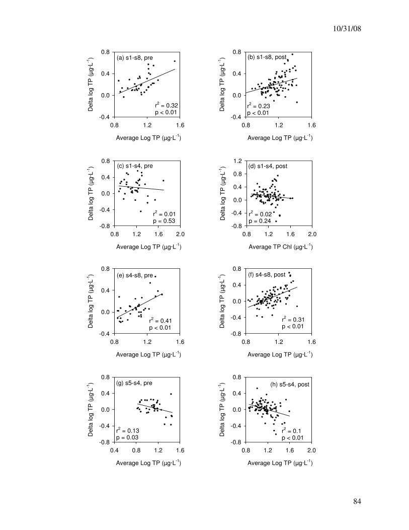
10/31/08
84
Average Log TP (µg·L-1
)
0.8 1.2 1.6
Delta log T
P (
µg·L
-1)
-0.4
0.0
0.4
0.8(a) s1-s8, pre
r2 = 0.32
p < 0.01
Average Log TP (µg·L-1
)
0.8 1.2 1.6
Delta log T
P (
µg·L
-1)
-0.4
0.0
0.4
0.8
r2 = 0.23
p < 0.01
(b) s1-s8, post
Average Log TP (µg·L-1
)
0.8 1.2 1.6
Delta log T
P (
µg·L
-1)
-0.4
0.0
0.4
0.8
(c) s1-s4, pre
r2 = 0.01
p = 0.53
Average Log TP (µg·L-1
)
0.8 1.2 1.6
Delta log T
P (
µg·L
-1)
-0.8
-0.4
0.0
0.4
0.8
(d) s1-s4, post
r2 = 0.02
p = 0.24
Average Log TP (µg·L-1
)
0.4 0.8 1.2 1.6
Delta log T
P (
µg·L
-1)
-0.8
-0.4
0.0
0.4
0.8
Average Log TP (µg·L-1
)
0.8 1.2 1.6 2.0
Delta log T
P (
µg·L
-1)
-0.8
-0.4
0.0
0.4
0.8
(e) s4-s8, pre (f) s4-s8, post
(g) s5-s4, pre (h) s5-s4, post
r2 = 0.41
p < 0.01
r2 = 0.31
p < 0.01
Average Log TP (µg·L-1
)
0.8 1.2 1.6 2.0
Delta log T
P (
µg·L
-1)
-0.8
-0.4
0.0
0.4
0.8
Average TP Chl (µg·L-1
)
0.8 1.2 1.6 2.0
Delta log T
P (
µg·L
-1)
-0.8
-0.4
0.0
0.4
0.8
1.2
r2 = 0.13
p = 0.03r2 = 0.1
p < 0.01
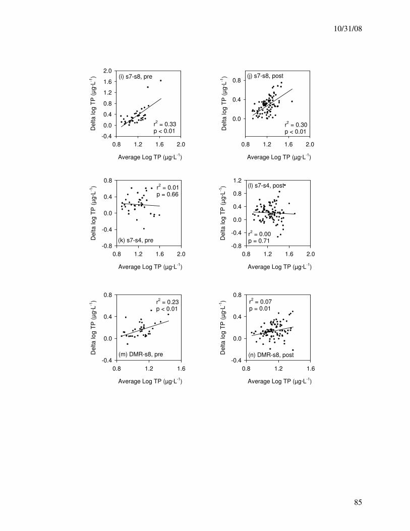
10/31/08
85
Average Log TP (µg·L-1
)
0.8 1.2 1.6 2.0
De
lta lo
g T
P (
µg·L
-1)
-0.4
0.0
0.4
0.8
1.2
1.6
2.0(i) s7-s8, pre
r2 = 0.33
p < 0.01
Average Log TP (µg·L-1
)
0.8 1.2 1.6 2.0
De
lta lo
g T
P (
µg·L
-1)
0.0
0.4
0.8
r2 = 0.30
p < 0.01
(j) s7-s8, post
(k) s7-s4, pre
r2 = 0.01
p = 0.66
(l) s7-s4, post
r2 = 0.00
p = 0.71
Average Log TP (µg·L-1
)
0.8 1.2 1.6 2.0
De
lta lo
g T
P (
µg
·L-1
)
-0.8
-0.4
0.0
0.4
0.8
Average Log TP (µg·L-1
)
0.8 1.2 1.6 2.0
De
lta lo
g T
P (
µg
·L-1
)
-0.8
-0.4
0.0
0.4
0.8
1.2
Average Log TP (µg·L-1
)
0.8 1.2 1.6
Delta
lo
g T
P (
µg
·L-1
)
-0.4
0.0
0.4
0.8
Average Log TP (µg·L-1
)
0.8 1.2 1.6
Delta
lo
g T
P (
µg
·L-1
)
-0.4
0.0
0.4
0.8
(m) DMR-s8, pre (n) DMR-s8, post
r2 = 0.23
p < 0.01r2 = 0.07
p = 0.01
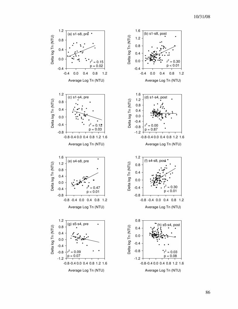
10/31/08
86
Average Log Tn (NTU)
-0.4 0.0 0.4 0.8 1.2
Delta log T
n (
NT
U)
-0.4
0.0
0.4
0.8
1.2(a) s1-s8, pre
r2 = 0.15
p = 0.02
Average Log Tn (NTU)
-0.4 0.0 0.4 0.8 1.2
Delta log T
n (
NT
U)
-0.4
0.0
0.4
0.8
1.2
1.6
r2 = 0.30
p < 0.01
(b) s1-s8, post
Average Log Tn (NTU)
-0.8 -0.4 0.0 0.4 0.8 1.2
Delta log T
n (
NT
U)
-0.8
-0.4
0.0
0.4
0.8
1.2
1.6
(c) s1-s4, pre
r2 = 0.12
p = 0.03
Average Log Tn (NTU)
-0.8 -0.4 0.0 0.4 0.8 1.2
Delta log T
n (
NT
U)
-0.8
-0.4
0.0
0.4
0.8
1.2
(d) s1-s4, post
r2 = 0.00
p = 0.87
Average Log Tn (NTU)
-0.8-0.4 0.0 0.4 0.8 1.2 1.6
Delta log T
n (
NT
U)
-1.2
-0.8
-0.4
0.0
0.4
0.8
1.2
Average Log Tn (NTU)
-0.8-0.4 0.0 0.4 0.8 1.2 1.6
Delta log T
n (
NT
U)
-1.2
-0.8
-0.4
0.0
0.4
0.8
(e) s4-s8, pre (f) s4-s8, post
(g) s5-s4, pre (h) s5-s4, post
r2 = 0.47
p < 0.01
r2 = 0.30
p < 0.01
Average Log Tn (NTU)
-0.8-0.4 0.0 0.4 0.8 1.2 1.6
Delta log T
n (
NT
U)
-0.8
-0.4
0.0
0.4
0.8
1.2
Average Log Tn (NTU)
-0.8-0.4 0.0 0.4 0.8 1.2 1.6
Delta log T
n (
NT
U)
-1.2
-0.8
-0.4
0.0
0.4
0.8
1.2
1.6
r2 = 0.09
p = 0.07r2 = 0.03
p = 0.08
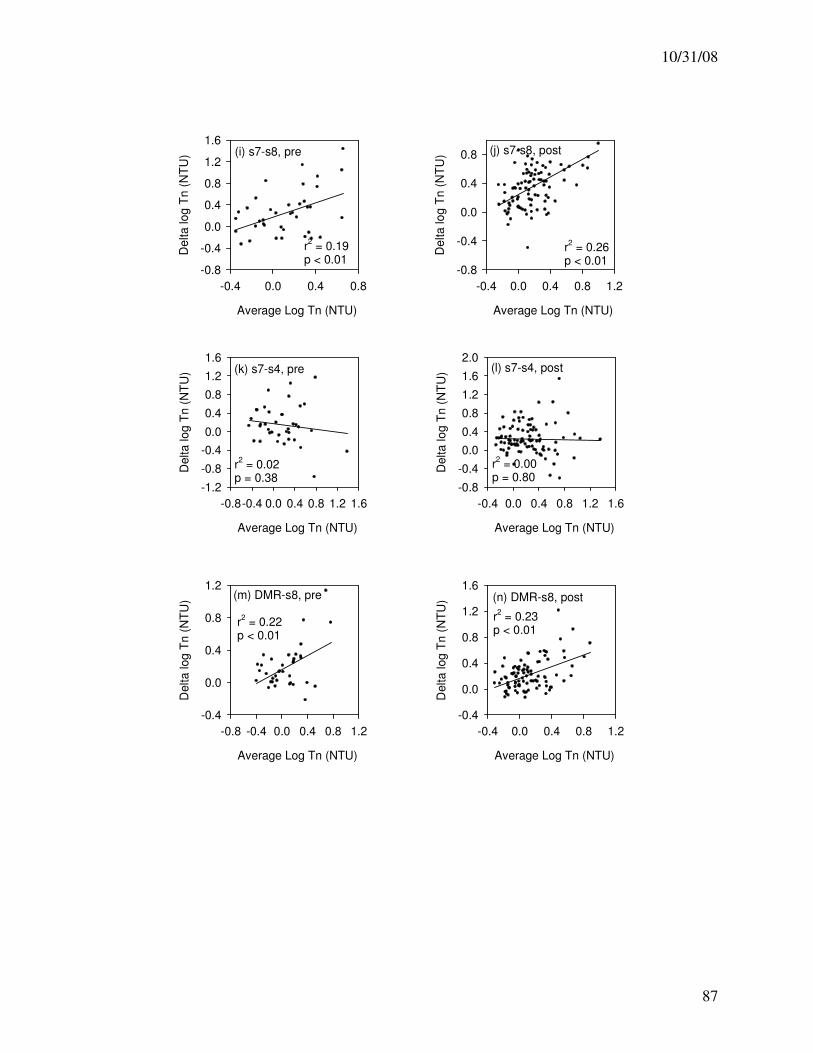
10/31/08
87
Average Log Tn (NTU)
-0.4 0.0 0.4 0.8
De
lta lo
g T
n (
NT
U)
-0.8
-0.4
0.0
0.4
0.8
1.2
1.6(i) s7-s8, pre
r2 = 0.19
p < 0.01
Average Log Tn (NTU)
-0.4 0.0 0.4 0.8 1.2
De
lta lo
g T
n (
NT
U)
-0.8
-0.4
0.0
0.4
0.8
r2 = 0.26
p < 0.01
(j) s7-s8, post
(k) s7-s4, pre
r2 = 0.02
p = 0.38
(l) s7-s4, post
r2 = 0.00
p = 0.80
Average Log Tn (NTU)
-0.8-0.4 0.0 0.4 0.8 1.2 1.6
Delta
lo
g T
n (
NT
U)
-1.2
-0.8
-0.4
0.0
0.4
0.8
1.2
1.6
Average Log Tn (NTU)
-0.4 0.0 0.4 0.8 1.2 1.6
Delta
lo
g T
n (
NT
U)
-0.8
-0.4
0.0
0.4
0.8
1.2
1.6
2.0
Average Log Tn (NTU)
-0.8 -0.4 0.0 0.4 0.8 1.2
Delta
log
Tn
(N
TU
)
-0.4
0.0
0.4
0.8
1.2
Average Log Tn (NTU)
-0.4 0.0 0.4 0.8 1.2
Delta
log
Tn
(N
TU
)
-0.4
0.0
0.4
0.8
1.2
1.6(m) DMR-s8, pre (n) DMR-s8, post
r2 = 0.22
p < 0.01
r2 = 0.23
p < 0.01

10/31/08
88
Appendix 4 – Nonparametric Analysis
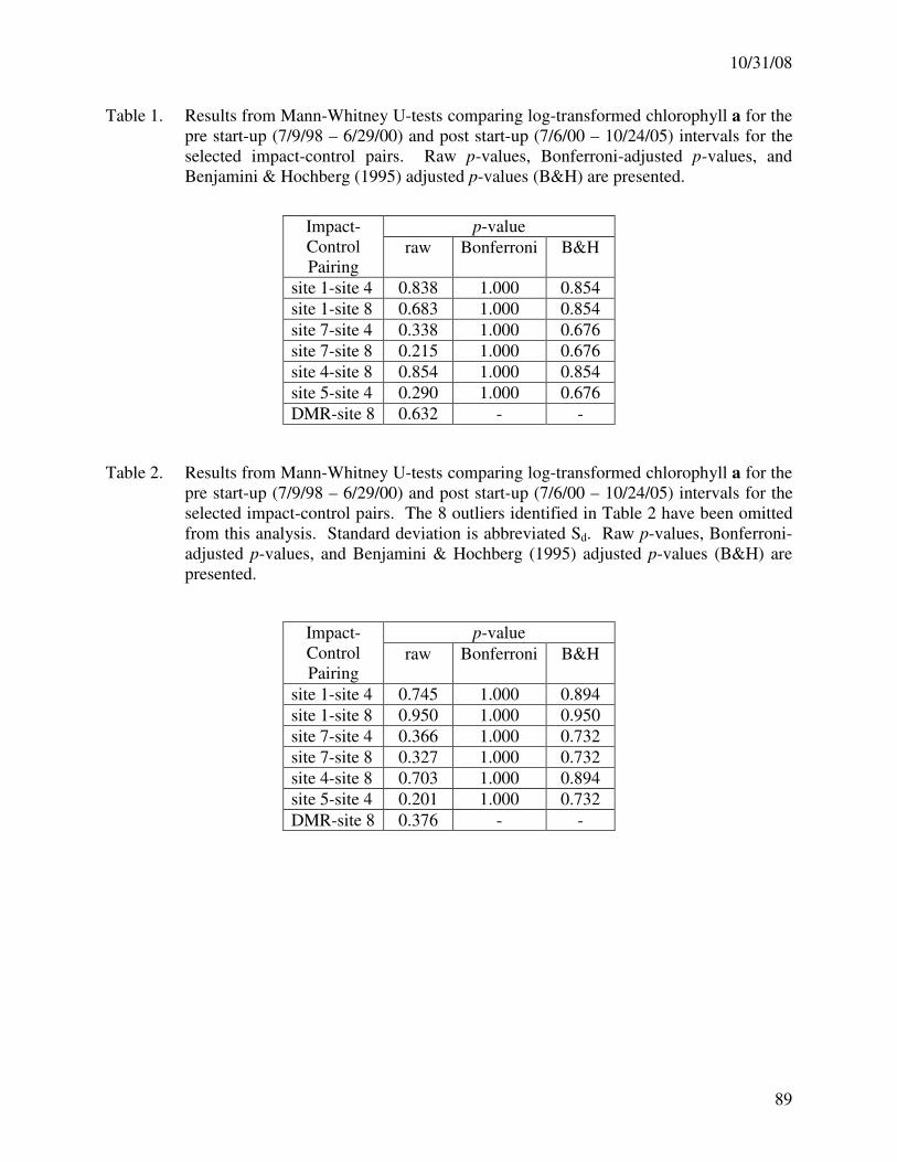
10/31/08
89
Table 1. Results from Mann-Whitney U-tests comparing log-transformed chlorophyll a for the
pre start-up (7/9/98 – 6/29/00) and post start-up (7/6/00 – 10/24/05) intervals for the
selected impact-control pairs. Raw p-values, Bonferroni-adjusted p-values, and
Benjamini & Hochberg (1995) adjusted p-values (B&H) are presented.
Impact-
Control
Pairing
p-value
raw Bonferroni B&H
site 1-site 4 0.838 1.000 0.854
site 1-site 8 0.683 1.000 0.854
site 7-site 4 0.338 1.000 0.676
site 7-site 8 0.215 1.000 0.676
site 4-site 8 0.854 1.000 0.854
site 5-site 4 0.290 1.000 0.676
DMR-site 8 0.632 - -
Table 2. Results from Mann-Whitney U-tests comparing log-transformed chlorophyll a for the
pre start-up (7/9/98 – 6/29/00) and post start-up (7/6/00 – 10/24/05) intervals for the
selected impact-control pairs. The 8 outliers identified in Table 2 have been omitted
from this analysis. Standard deviation is abbreviated Sd. Raw p-values, Bonferroni-
adjusted p-values, and Benjamini & Hochberg (1995) adjusted p-values (B&H) are
presented.
Impact-
Control
Pairing
p-value
raw Bonferroni B&H
site 1-site 4 0.745 1.000 0.894
site 1-site 8 0.950 1.000 0.950
site 7-site 4 0.366 1.000 0.732
site 7-site 8 0.327 1.000 0.732
site 4-site 8 0.703 1.000 0.894
site 5-site 4 0.201 1.000 0.732
DMR-site 8 0.376 - -
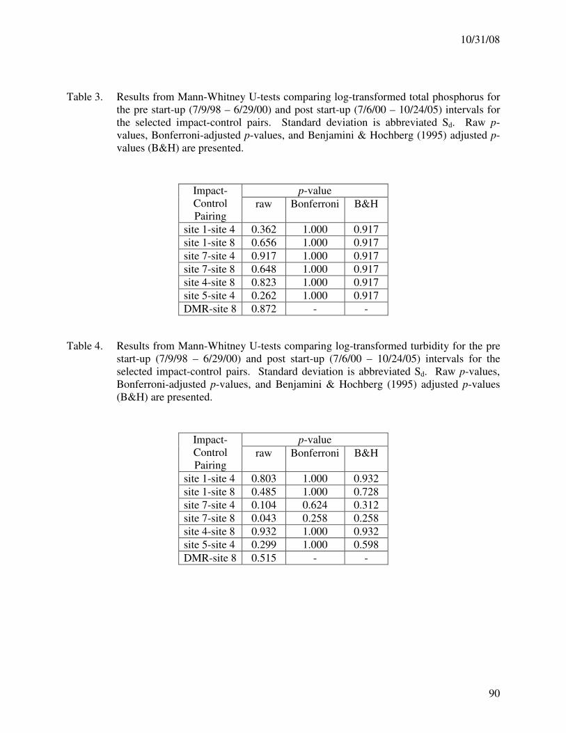
10/31/08
90
Table 3. Results from Mann-Whitney U-tests comparing log-transformed total phosphorus for
the pre start-up (7/9/98 – 6/29/00) and post start-up (7/6/00 – 10/24/05) intervals for
the selected impact-control pairs. Standard deviation is abbreviated Sd. Raw p-
values, Bonferroni-adjusted p-values, and Benjamini & Hochberg (1995) adjusted p-
values (B&H) are presented.
Impact-
Control
Pairing
p-value
raw Bonferroni B&H
site 1-site 4 0.362 1.000 0.917
site 1-site 8 0.656 1.000 0.917
site 7-site 4 0.917 1.000 0.917
site 7-site 8 0.648 1.000 0.917
site 4-site 8 0.823 1.000 0.917
site 5-site 4 0.262 1.000 0.917
DMR-site 8 0.872 - -
Table 4. Results from Mann-Whitney U-tests comparing log-transformed turbidity for the pre
start-up (7/9/98 – 6/29/00) and post start-up (7/6/00 – 10/24/05) intervals for the
selected impact-control pairs. Standard deviation is abbreviated Sd. Raw p-values,
Bonferroni-adjusted p-values, and Benjamini & Hochberg (1995) adjusted p-values
(B&H) are presented.
Impact-
Control
Pairing
p-value
raw Bonferroni B&H
site 1-site 4 0.803 1.000 0.932
site 1-site 8 0.485 1.000 0.728
site 7-site 4 0.104 0.624 0.312
site 7-site 8 0.043 0.258 0.258
site 4-site 8 0.932 1.000 0.932
site 5-site 4 0.299 1.000 0.598
DMR-site 8 0.515 - -

10/31/08
91
Appendix 5 – Raw Time Series Plots
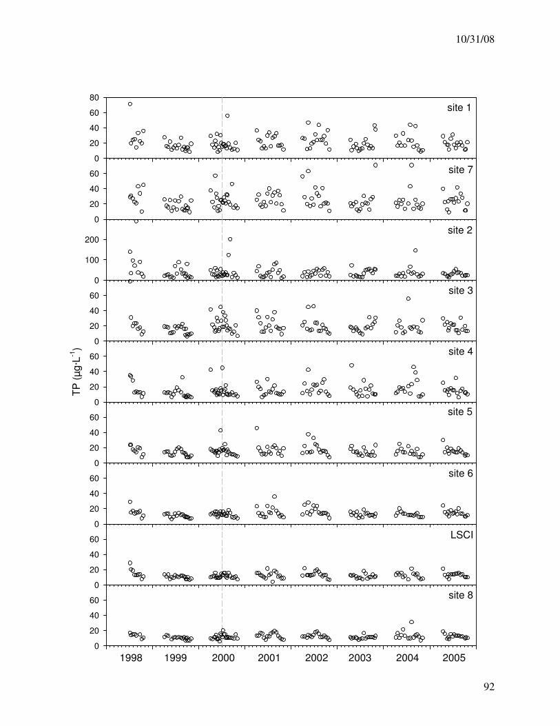
10/31/08
92
0
20
40
60
80
site 1
0
20
40
60 site 7
0
100
200site 2
0
20
40
60
TP
(µ
g·L
-1)
0
20
40
60
0
20
40
60
site 3
site 4
site 5
0
20
40
60site 6
0
20
40
60 LSCI
0
20
40
60site 8
1998 1999 2000 2001 2002 2003 2004 2005
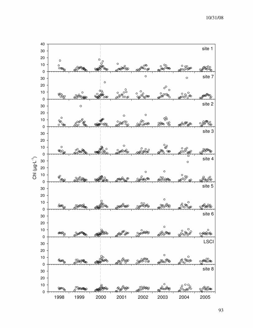
10/31/08
93
0
10
20
30
40
site 1
0
10
20
30 site 7
0
10
20
30 site 2
0
10
20
30
Chl (µ
g·L
-1)
0
10
20
30
0
10
20
30
site 3
site 4
site 5
0
10
20
30site 6
0
10
20
30 LSCI
0
10
20
30site 8
1998 1999 2000 2001 2002 2003 2004 2005
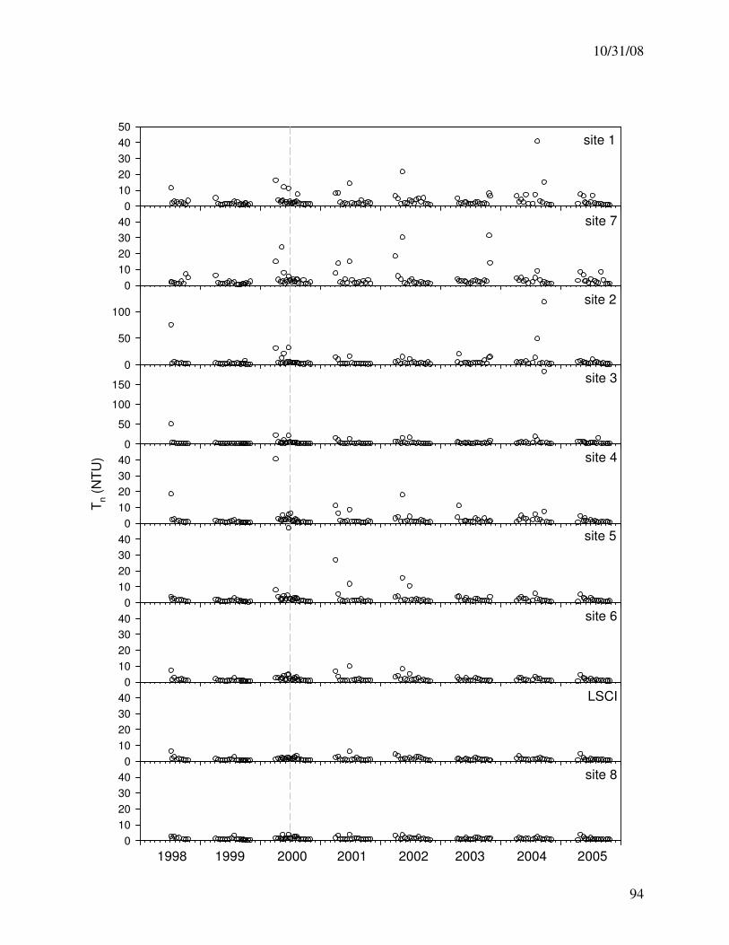
10/31/08
94
0
10
20
30
40
50
site 1
0
10
20
30
40 site 7
0
50
100site 2
0
50
100
150
Tn (
NT
U)
0
10
20
30
40
0
10
20
30
40
site 3
site 4
site 5
0
10
20
30
40 site 6
0
10
20
30
40 LSCI
0
10
20
30
40 site 8
1998 1999 2000 2001 2002 2003 2004 2005


![)( CORNELL REPORTS - [email protected] - Cornell University](https://img.pdfslide.net/doc/110x75/6206299f8c2f7b17300506a0/-cornell-reports-emailprotected-cornell-university.jpg)