Sequencing costs have fallen so dramatically that a sin-gle laboratory can now afford to sequence large, even human-sized, genomes. Ironically, although sequencing has become easy, in many ways, genome annotation has become more challenging. Several factors are respon-sible for this. First, the shorter read lengths of second-generation sequencing platforms mean that current genome assemblies rarely attain the contiguity of the classic shotgun assemblies of the Drosophila mela-nogaster 1,2 or human genomes3,4. Second, the exotic nature of many recently sequenced genomes also pre-sents annotation challenges, especially for gene finding. Whereas the first generation of genome projects had recourse to large numbers of pre-existing gene mod-els, the contents of today’s genomes are often terra incognita. This makes it difficult to train, optimize and configure gene prediction and annotation tools.

A third new challenge is posed by the need to update and merge annotation data sets. RNA-sequencing data (RNA-seq data)5–8 provide an obvious means for updating older annotation data sets; however, doing so is not trivial. It is also not straightforward to ascertain whether the result improves on the original annotation. Furthermore, it is not unusual today for multiple groups to annotate the same genome using different annota-tion procedures. Merging these to produce a consensus annotation data set is a complex task.

Finally, the demographics of genome annotation projects are changing as well. Unlike the massive genome projects of the past, today’s genome annota-tion projects are usually smaller-scale affairs and often involve researchers who have little bioinformatics and computational biology expertise. Eukaryotic genome annotation is not a point-and-click process; however,

with some basic UNIX skills, ‘do-it-yourself ’ genome annotation projects are quite feasible using present-day tools. Here we provide an overview of the eukary-otic genome annotation process, describe the available toolsets and outline some best-practice approaches.

Assembly and annotation: an overviewAssembly. The first step towards the successful annota-tion of any genome is determining whether its assem-bly is ready for annotation. Several summary statistics are used to describe the completeness and contiguity of a genome assembly, and by far the most important is N50 (BOX 1). Other useful assembly statistics are the average gap size of a scaffold and the average number of gaps per scaffold (BOX 1). Most current genomes are ‘standard draft’ assemblies, meaning that they meet minimum standards for submission to public data-bases9. However, a ‘high-quality draft’ assembly9 is a much better target for annotation, as it is at least 90% complete.

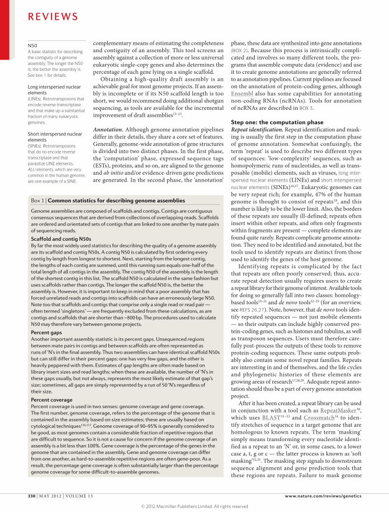
Although there are no strict rules, an assembly with an N50 scaffold length that is gene-sized is a decent target for annotation. The reason is simple: if the scaffold N50 is around the median gene length, then ~50% of the genes will be contained on a single scaf-fold; these complete genes, together with fragments from the rest of the genome, will provide a sizable resource for downstream analyses10,11. As can be seen in FIG. 1, median gene lengths are roughly propor-tional to genome size. Thus, if the size of the genome of interest is known, it is possible to use this figure to obtain a rough estimate of gene lengths and hence to obtain an estimate of the minimum N50 scaffold length for annotation. CEGMA12 provides another,

Department of Human Genetics, Eccles Institute of Human Genetics, School of Medicine, University of Utah, Salt Lake City, Utah 84112‑5330, USA. Correspondence to M.Y. e‑mail: myandell@genetics.utah.edu doi:10.1038/nrg3174

Genome annotation A term used to describe two distinct processes. ‘Structural’ genome annotation is the process of identifying genes and their intron–exon structures. ‘Functional’ genome annotation is the process of attaching meta-data such as gene ontology terms to structural annotations. This Review focuses on structural annotation.

RNA-sequencing data (RNA-seq data). Data sets derived from the shotgun sequencing of a whole transcriptome using next-generation sequencing (NGS) techniques. RNA-seq data are the NGS equivalent of expressed sequence tags generated by the Sanger sequencing method.

A beginner’s guide to eukaryotic genome annotationMark Yandell and Daniel Ence

Abstract | The falling cost of genome sequencing is having a marked impact on the research community with respect to which genomes are sequenced and how and where they are annotated. Genome annotation projects have generally become small-scale affairs that are often carried out by an individual laboratory. Although annotating a eukaryotic genome assembly is now within the reach of non-experts, it remains a challenging task. Here we provide an overview of the genome annotation process and the available tools and describe some best-practice approaches.

S T U DY D E S I G N S

R E V I E W S

NATURE REVIEWS | GENETICS VOLUME 13 | MAY 2012 | 329

© 2012 Macmillan Publishers Limited. All rights reserved

N50 A basic statistic for describing the contiguity of a genome assembly. The longer the N50 is, the better the assembly is. See box 1 for details.

Long interspersed nuclear elements (LINEs). Retrotransposons that encode reverse transcriptase and that make up a substantial fraction of many eukaryotic genomes.

Short interspersed nuclear elements (SINEs). Retrotransposons that do no encode reverse transcriptase and that parasitize LINE elements. ALU elements, which are very common in the human genome, are one example of a SINE.

complementary means of estimating the completeness and contiguity of an assembly. This tool screens an assembly against a collection of more or less universal eukaryotic single-copy genes and also determines the percentage of each gene lying on a single scaffold.

Obtaining a high-quality draft assembly is an achievable goal for most genome projects. If an assem-bly is incomplete or if its N50 scaffold length is too short, we would recommend doing additional shotgun sequencing, as tools are available for the incremental improvement of draft assemblies13–15.

Annotation. Although genome annotation pipelines differ in their details, they share a core set of features. Generally, genome-wide annotation of gene structures is divided into two distinct phases. In the first phase, the ‘computation’ phase, expressed sequence tags (ESTs), proteins, and so on, are aligned to the genome and ab initio and/or evidence-driven gene predictions are generated. In the second phase, the ‘annotation’

phase, these data are synthesized into gene annotations (BOX 2). Because this process is intrinsically compli-cated and involves so many different tools, the pro-grams that assemble compute data (evidence) and use it to create genome annotations are generally referred to as annotation pipelines. Current pipelines are focused on the annotation of protein-coding genes, although Ensembl also has some capabilities for annotating non-coding RNAs (ncRNAs). Tools for annotation of ncRNAs are described in BOX 3.

Step one: the computation phaseRepeat identification. Repeat identification and mask-ing is usually the first step in the computation phase of genome annotation. Somewhat confusingly, the term ‘repeat’ is used to describe two different types of sequences: ‘low-complexity’ sequences, such as homopolymeric runs of nucleotides, as well as trans-posable (mobile) elements, such as viruses, long inter-spersed nuclear elements (LINEs) and short interspersed nuclear elements (SINEs)16,17. Eukaryotic genomes can be very repeat rich; for example, 47% of the human genome is thought to consist of repeats18, and this number is likely to be the lower limit. Also, the borders of these repeats are usually ill-defined; repeats often insert within other repeats, and often only fragments within fragments are present — complete elements are found quite rarely. Repeats complicate genome annota-tion. They need to be identified and annotated, but the tools used to identify repeats are distinct from those used to identify the genes of the host genome.

Identifying repeats is complicated by the fact that repeats are often poorly conserved; thus, accu-rate repeat detection usually requires users to create a repeat library for their genome of interest. Available tools for doing so generally fall into two classes: homology- based tools19–21 and de novo tools22–25 (for an overview, see REFS 26,27). Note, however, that de novo tools iden-tify repeated sequences — not just mobile elements — so their outputs can include highly conserved pro-tein-coding genes, such as histones and tubulins, as well as transposon sequences. Users must therefore care-fully post-process the outputs of these tools to remove protein-coding sequences. These same outputs prob-ably also contain some novel repeat families. Repeats are interesting in and of themselves, and the life cycles and phylogenetic histories of these elements are growing areas of research17,28,29. Adequate repeat anno-tation should thus be a part of every genome annotation project.

After it has been created, a repeat library can be used in conjunction with a tool such as RepeatMasker30, which uses BLAST31–33 and Crossmatch34 to iden-tify stretches of sequence in a target genome that are homologous to known repeats. The term ‘masking’ simply means transforming every nucleotide identi-fied as a repeat to an ‘N’ or, in some cases, to a lower case a, t, g or c — the latter process is known as ‘soft masking’32,35. The masking step signals to downstream sequence alignment and gene prediction tools that these regions are repeats. Failure to mask genome

Box 1 | Common statistics for describing genome assemblies

Genome assemblies are composed of scaffolds and contigs. Contigs are contiguous consensus sequences that are derived from collections of overlapping reads. Scaffolds are ordered and orientated sets of contigs that are linked to one another by mate pairs of sequencing reads.

Scaffold and contig N50sBy far the most widely used statistics for describing the quality of a genome assembly are its scaffold and contig N50s. A contig N50 is calculated by first ordering every contig by length from longest to shortest. Next, starting from the longest contig, the lengths of each contig are summed, until this running sum equals one-half of the total length of all contigs in the assembly. The contig N50 of the assembly is the length of the shortest contig in this list. The scaffold N50 is calculated in the same fashion but uses scaffolds rather than contigs. The longer the scaffold N50 is, the better the assembly is. However, it is important to keep in mind that a poor assembly that has forced unrelated reads and contigs into scaffolds can have an erroneously large N50. Note too that scaffolds and contigs that comprise only a single read or read pair — often termed ‘singletons’ — are frequently excluded from these calculations, as are contigs and scaffolds that are shorter than ~800 bp. The procedures used to calculate N50 may therefore vary between genome projects.

Percent gaps Another important assembly statistic is its percent gaps. Unsequenced regions between mate pairs in contigs and between scaffolds are often represented as runs of ‘N’s in the final assembly. Thus two assemblies can have identical scaffold N50s but can still differ in their percent gaps: one has very few gaps, and the other is heavily peppered with them. Estimates of gap lengths are often made based on library insert sizes and read lengths; when these are available, the number of ‘N’s in these gaps usually, but not always, represents the most likely estimate of that gap’s size; sometimes, all gaps are simply represented by a run of 50 ‘N’s regardless of their size.

Percent coverage Percent coverage is used in two senses: genome coverage and gene coverage. The first number, genome coverage, refers to the percentage of the genome that is contained in the assembly based on size estimates; these are usually based on cytological techniques116,117. Genome coverage of 90–95% is generally considered to be good, as most genomes contain a considerable fraction of repetitive regions that are difficult to sequence. So it is not a cause for concern if the genome coverage of an assembly is a bit less than 100%. Gene coverage is the percentage of the genes in the genome that are contained in the assembly. Gene and genome coverage can differ from one another, as hard-to-assemble repetitive regions are often gene-poor. As a result, the percentage gene coverage is often substantially larger than the percentage genome coverage for some difficult-to-assemble genomes.

R E V I E W S

330 | MAY 2012 | VOLUME 13 www.nature.com/reviews/genetics

© 2012 Macmillan Publishers Limited. All rights reserved

Nature Reviews | Genetics

Escherichia coli

Saccharomycescerevisiae

Schizosaccharomycespombe

Caenorhabditiselegans

Arabidopsisthaliana

Volvoxcarteri

Drosophila melanogaster

Citrus clementina

Takifugurubripes

Oryzasativa

Populustrichocarpa

Eucalyptusgrandis

Gallus gallus

Danio rerio

Ornithorhynchusanatinus

Zea mays

Ailuropodamelanoleuca

Musmusculus

Homosapiens

1.0 1.5 2.0 2.5 3.0 3.50.5

3.0

2.8

3.2

3.4

3.6

3.8

4.0

4.2

log10 (genome size) (Mbp)

log 10

(gen

e si

ze) (

bp)

Fungi

Invertebrates

Plants

Bacteria

Mammalian vertebrates

Non−mammalian vertebrates

Figure 1 | Genome and gene sizes for a representative set of genomes. Gene size is plotted as a function of genome size for some representative bacteria, fungi, plants and animals. This figure illustrates a simple rule of thumb: in general, bigger genomes have bigger genes. Thus, accurate annotation of a larger genome requires a more contiguous genome assembly in order to avoid splitting genes across scaffolds. Note too that although the human and mouse genomes deviate from the simple linear model shown here, the trend still holds. Their unusually large genes are likely to be a consequence of the mature status of their annotations, which are much more complete as regards annotation of alternatively spliced transcripts and untranslated regions than those of most other genomes.

sequences can be catastrophic. Left unmasked, repeats can seed millions of spurious BLAST alignments32, pro-ducing false evidence for gene annotations. Worse still, many transposon open reading frames (ORFs) look like true host genes to gene predictors, causing portions of transposon ORFs to be added as additional exons to gene predictions, completely corrupting the final gene annotations. Good repeat masking is thus crucial for the accurate annotation of protein-coding genes.

Evidence alignment. After repeat masking, most pipe-lines align proteins, ESTs and RNA-seq data to the genome assembly. These sequences include previously identified transcripts and proteins from the organism whose genome is being annotated. Sequences from other organisms are also included; generally, these are restricted to proteins, as these retain substantial

sequence similarity over much greater spans of evo-lutionary time than nucleotide sequences do. In prin-ciple, TBLASTX31,32,36 can be used to align ESTs and RNA-seq data from phylogenetically distant organisms but, owing to high computational costs, this is only done rarely.

UniProtKB/SwissProt 37–39 is an excellent core resource for protein sequences. As SwissProt is restricted to highly curated proteins, many users might want to supplement this database with the proteomes of related, previously annotated genomes. One easy way to assemble additional protein and EST data sets is to download sequences from related organisms using the NCBI taxonomy browser40,41.

EST and protein sequence data sets are often aligned to the genome in a two-tiered process. Frequently, BLAST31,32,36 and BLAT42 are used to

R E V I E W S

NATURE REVIEWS | GENETICS VOLUME 13 | MAY 2012 | 331

© 2012 Macmillan Publishers Limited. All rights reserved

Box 2 | Gene prediction versus gene annotation

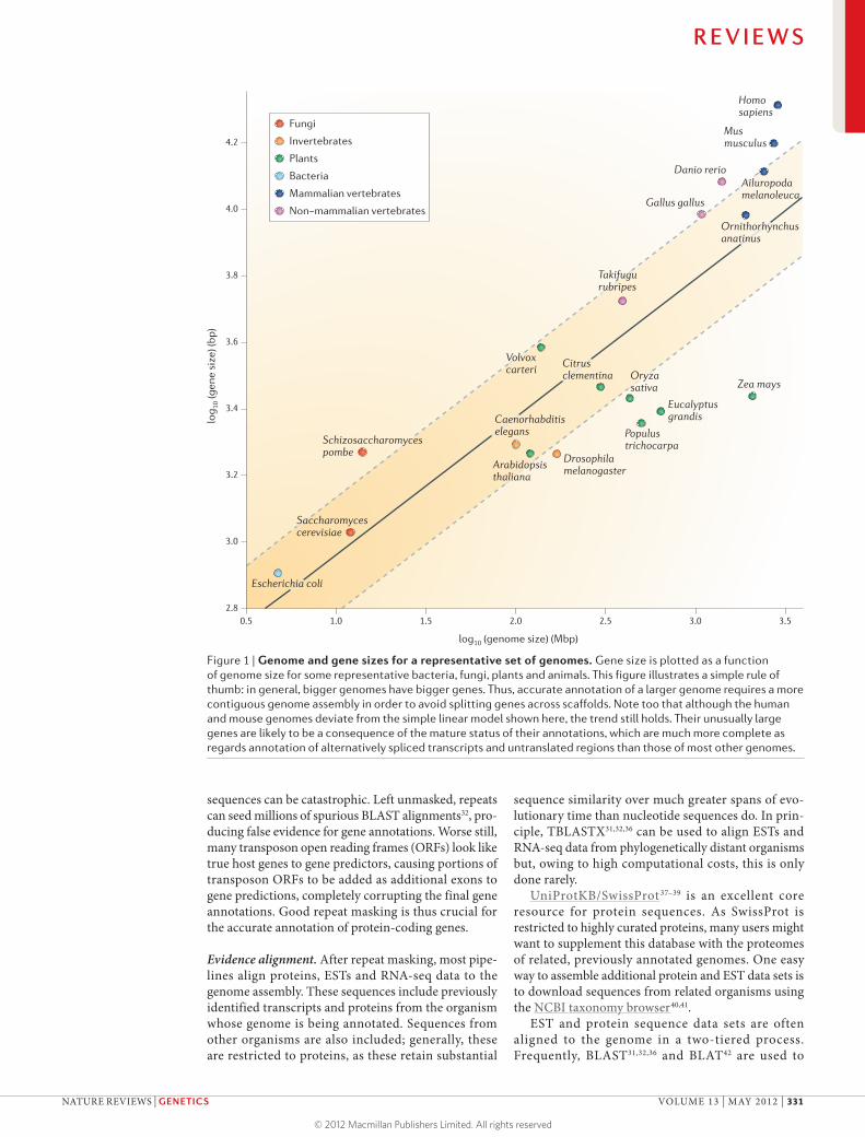
Although the terms ‘gene prediction’ and ‘gene annotation’ are often used as if they are synonyms, they are not. With a few exceptions, gene predictors find the single most likely coding sequence (CDS) of a gene and do not report untranslated regions (UTRs) or alternatively spliced variants. Gene prediction is therefore a somewhat misleading term. A more accurate description might be ‘canonical CDS prediction’.

Gene annotations, conversely, generally include UTRs, alternative splice isoforms and have attributes such as evidence trails. The figure shows a genome annotation and its associated evidence. Terms in parentheses are the names of commonly used software tools for assembling particular types of evidence. Note that the gene annotation (shown in blue) captures both alternatively spliced forms and the 5′ and 3′UTRs suggested by the evidence. By contrast, the gene prediction that is generated by SNAP (shown in green) is incorrect as regards the gene’s 5′ exons and start-of-translation site and, like most gene-predictors, it predicts only a single transcript with no UTR.

Gene annotation is thus a more complex task than gene prediction. A pipeline for genome annotation must not only deal with heterogeneous types of evidence in the form of the expressed sequence tags (ESTs), RNA-seq data, protein homologies and gene predictions, but it must also synthesize all of these data into coherent gene models and produce an output that describes its results in sufficient detail for these outputs to become suitable inputs to genome browsers and annotation databases.

Nature Reviews | Genetics

229,500 229,000 228,500 228,000 227,500 226,500227,000bp

5′UTR 3′UTR

Gene annotation resultingfrom synthesizing all available evidence (two alternative splice forms)

Protein evidence(BLASTX)

mRNA or EST evidence(Exonerate)

Gene prediction(SNAP)

Start codon Stop codon

Percent similarity The percent similarity of a sequence alignment refers to the percentage of positive scoring aligned bases or amino acids in a nucleotide or protein alignment, respectively. The term positive scoring refers to the score assigned to the paired nucleotides or amino acids by the scoring matrix that is used to align the sequences.

Percent identity The percent identity of a sequence alignment refers to the percentage of identical aligned bases or amino acids in a nucleotide or protein alignment, respectively.

identify approximate regions of homology rapidly. These alignments are usually filtered to identify and to remove marginal alignments on the basis of met-rics such as percent similarity or percent identity. After filtering, the remaining data are sometimes clustered to identify overlapping alignments and predictions. Clustering has two purposes. First, it groups diverse computational results into a single cluster of data, all supporting the same gene. Second, it identifies and purges redundant evidence; highly expressed genes, for example, may be supported by hundreds if not thousands of identical ESTs.

The term ‘polishing’ is sometimes used to describe the next phase of the alignment process. After cluster-ing, highly similar sequences identified by BLAST and BLAT are realigned to the target genome in order to obtain greater precision at exon boundaries. BLAST, for example, although rapid, has no model for splice sites, and so the edges of its sequence alignments are only rough approximations of exon boundaries43. For this reason, splice-site-aware alignment algorithms, such as Splign44, Spidey45, sim4 (REF. 46) and Exonerate43, are often used to realign matching and highly similar ESTs, mRNAs and proteins to the genomic

input sequence. Although these programs take longer to run, they provide the annotation pipeline with much improved information about splice sites and exon boundaries.

Of all forms of evidence, RNA-seq data have the greatest potential to improve the accuracy of gene annotations, as these data provide copious evidence for better delimitation of exons, splice sites and alter-natively spliced exons. However, these data can be difficult to use because of their large size and com-plexity. The use of RNA-seq data currently lies at the cutting edge of genome annotation, and the available toolset is evolving quickly47. Currently, RNA-seq reads are usually handled in two ways. They can be assem-bled de novo — that is, independently of the genome — using tools such as ABySS48, SOAPdenovo49 and Trinity50; the resulting transcripts are then realigned to the genome in the same way as ESTs. Alternatively, the RNA-seq data can be directly aligned to the genome using tools such as TopHat51, GSNAP52 or Scripture53 followed by the assembly of alignments (rather than reads) into transcripts using tools such as Cufflinks54. See REF. 55 for guidance on the best way to use TopHat with Cufflinks.

R E V I E W S

332 | MAY 2012 | VOLUME 13 www.nature.com/reviews/genetics

© 2012 Macmillan Publishers Limited. All rights reserved

Opinions differ as to the best approach for using RNA-seq data, and the most promising avenue will probably heavily depend on both genome biology (for example, gene density) and the contiguity and com-pleteness of the genome assembly. Gene density is an important consideration. If genes are closely spaced in the genome, then tools such as Cufflinks54 some-times erroneously merge RNA-seq reads from neigh-bouring genes. In such cases, de novo assembly of the RNA-seq data mitigates the problem; in fact, Trinity50 is designed to deal with this issue. Several annotation pipelines are now compatible with RNA-seq data: these include PASA56, which uses inchworm50 outputs, and MAKER10, which can operate directly from Cufflinks54 outputs or can use preassembled RNA-seq data.

Ab initio gene prediction. When gene predictors57–60 first became available in the 1990s (see REF. 61 for an overview), they revolutionized genome analyses because they provided a fast and easy means to identify genes in assembled DNA sequences. These tools are often referred to as ab initio gene predictors because they use mathematical models rather than external evidence (such as EST and protein alignments) to identify genes and to determine their intron–exon structures.

The great advantage of ab initio gene predictors for annotation is that, in principle, they need no external evidence to identify a gene or to determine its intron–exon structure. However, these tools have practical limitations from an annotation perspective.

For instance, most gene predictors find the single most likely coding sequence (CDS) and do not report untranslated regions (UTRs) or alternatively spliced transcripts (BOX 2). Training is also an issue; ab initio gene predictors use organism-specific genomic traits, such as codon frequencies and distributions of intron–exon lengths, to distinguish genes from intergenic regions and to determine intron–exon structures. Most gene predictors come with precalculated param-eter files that contain such information for a few classic genomes, such as Caenorhabditis elegans, D. mela-nogaster, Arabidopsis thaliana, humans and mice. However, unless your genome is very closely related to an organism for which precompiled parameter files are available, the gene predictor needs to be trained on the genome that is under study, as even closely related organisms can differ with respect to intron lengths, codon usage and GC content62.

Given enough training data, the gene-level sensi-tivity of ab initio tools can approach 100%63,64 (BOX 4). However, the accuracy of the predicted intron–exon structures is usually much lower, ~60–70%. It is also important to understand that large numbers of pre-existing, high-quality gene models and near base-perfect genome assemblies are usually required to produce highly accurate gene predictions63,65; such data sets are rarely available for newly sequenced genomes.

In principle, alignments of ESTs, RNA-seq and protein sequences to a genome can be used to train gene predictors even in the absence of pre-existing reference gene models. Although many popular gene predictors can be trained in this way, doing so often requires the user to have some basic programming skills. The MAKER pipeline provides a simplified process for training the predictors Augustus66,67 and SNAP62 using the EST, protein and mRNA-seq align-ments that MAKER has produced10,56. An alternative is to use GeneMark-ES68,69: a self-training, but sometimes less-accurate, algorithm69,70.

Evidence-driven gene prediction. In recent years, the distinction between ab initio prediction and gene annotation has been blurred. Many ab initio tools, such as TwinScan71, FGENESH72, Augustus, Gnomon73, GAZE74 and SNAP, can use external evidence to improve the accuracy of their predictions. ESTs, for example, can be used to identify exon boundaries unambiguously. This process is often referred to as evidence-driven (in contrast to ab initio) gene pre-diction. Evidence-driven gene prediction has great potential to improve the quality of gene prediction in newly sequenced genomes, but in practice it can be difficult to use. ESTs and proteins must first be aligned to the genome; RNA-seq data must be aligned too, if they are available. Splice sites must then be identified, and the assembled evidence must be post-processed before a synopsis of these data can be passed to the gene finder. In practice, this is a lot of work, requir-ing a lot of specialized software. In fact, it is one of the main obstacles that genome annotation pipelines attempt to overcome.

Box 3 | Non-coding RNAs

Non-coding RNA (ncRNA) annotation is still in its infancy compared with protein-coding gene annotation, but it is advancing rapidly. The heterogeneity and poorly conserved nature of many ncRNA genes present major challenges for annotation pipelines. Unlike protein-encoding genes, ncRNAs are usually not well-conserved at the primary sequence level; even when they are, nucleotide homologies are not as easily detected as protein homologies, which limits the power of evidence-based approaches.

One common approach is to identify ncRNA genes using conserved secondary structures and motifs. Established examples of these types of tools include tRNAscan-SE118 and Snoscan119. MicroRNA (miRNA) gene finders are also available120. A more general approach is first to align nucleotide sequences — genomic, RNA-seq and ESTs — from closely related organisms to the target genome and then search these for signs of conserved secondary structures. This is a complex process, however, and can require substantial computational resources; qRNA is one such tool121, another is StemLoc122. Be aware that these tools have high false-positive rates. RNA sequencing is also greatly aiding ncRNA identification. For example, miRNAs can be directly identified using specialized RNA preps and sequencing protocols123,124. Even with such sophisticated tools and techniques, distinguishing between bona fide ncRNA genes, spurious transcription and poorly conserved protein-encoding genes that produce small peptides remains difficult, especially in the cases of long intergenic non-coding RNAs (lincRNAs)125,126 and expressed pseudogenes127,128.

Another approach is to annotate possible ncRNA genes liberally and then use Infernal129 and Rfam114 to triage and classify these genes based on primary and secondary sequence similarities. Even with these resources, however, many ncRNAs will remain unclassifiable. Currently, ncRNA annotation is cutting edge, and those using ncRNA annotations should bear in mind that ncRNA annotation accuracies are generally much lower than those of their protein-coding counterparts.

R E V I E W S

NATURE REVIEWS | GENETICS VOLUME 13 | MAY 2012 | 333

© 2012 Macmillan Publishers Limited. All rights reserved

Nature Reviews | Genetics

A

Prediction 1

Prediction 2

SN SP AC

1 (1) 1 (1) 1 (1)

0.63 (0.33) 1 (0.5) 0.81 (0.42)

Reference gene model

Bb

Ba

EvidenceEST

Ab initio gene predictions

Protein

Annotation 1

Annotation 2

AED

0.2

0.6

Intron Exon

Gap Alignment

Intron Exon UTR

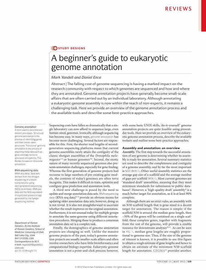
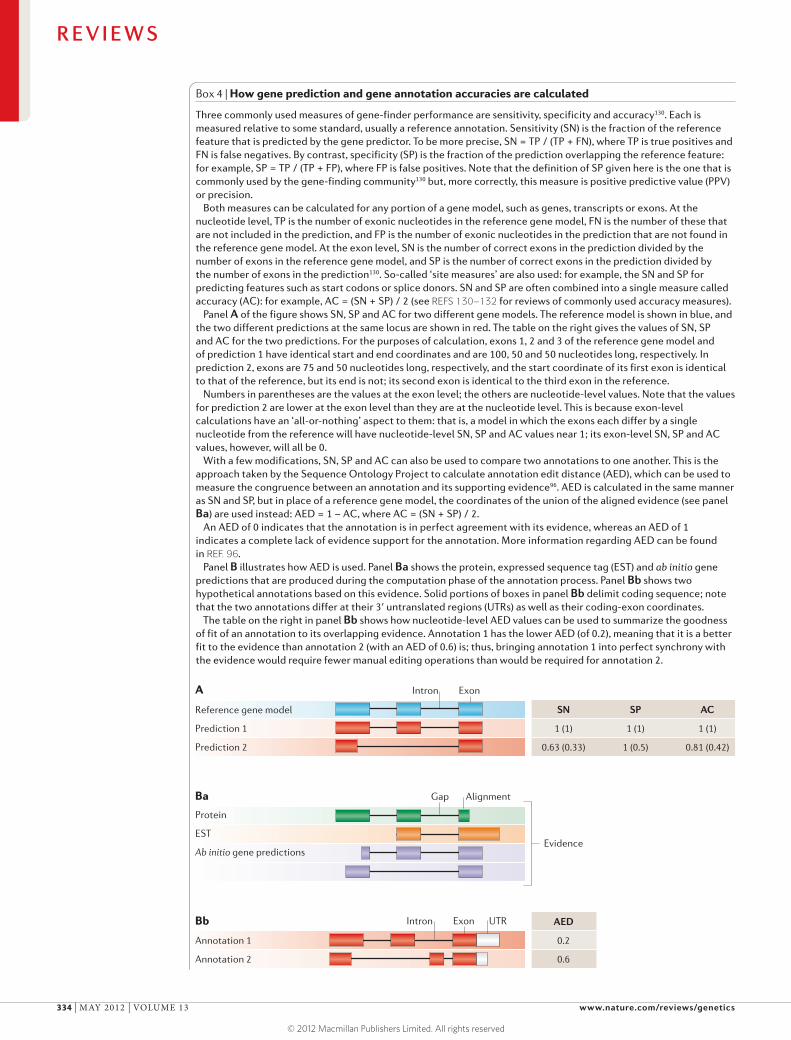
Box 4 | How gene prediction and gene annotation accuracies are calculated

Three commonly used measures of gene-finder performance are sensitivity, specificity and accuracy130. Each is measured relative to some standard, usually a reference annotation. Sensitivity (SN) is the fraction of the reference feature that is predicted by the gene predictor. To be more precise, SN = TP / (TP + FN), where TP is true positives and FN is false negatives. By contrast, specificity (SP) is the fraction of the prediction overlapping the reference feature: for example, SP = TP / (TP + FP), where FP is false positives. Note that the definition of SP given here is the one that is commonly used by the gene-finding community130 but, more correctly, this measure is positive predictive value (PPV) or precision.

Both measures can be calculated for any portion of a gene model, such as genes, transcripts or exons. At the nucleotide level, TP is the number of exonic nucleotides in the reference gene model, FN is the number of these that are not included in the prediction, and FP is the number of exonic nucleotides in the prediction that are not found in the reference gene model. At the exon level, SN is the number of correct exons in the prediction divided by the number of exons in the reference gene model, and SP is the number of correct exons in the prediction divided by the number of exons in the prediction130. So-called ‘site measures’ are also used: for example, the SN and SP for predicting features such as start codons or splice donors. SN and SP are often combined into a single measure called accuracy (AC): for example, AC = (SN + SP) / 2 (see REFS 130–132 for reviews of commonly used accuracy measures).

Panel A of the figure shows SN, SP and AC for two different gene models. The reference model is shown in blue, and the two different predictions at the same locus are shown in red. The table on the right gives the values of SN, SP and AC for the two predictions. For the purposes of calculation, exons 1, 2 and 3 of the reference gene model and of prediction 1 have identical start and end coordinates and are 100, 50 and 50 nucleotides long, respectively. In prediction 2, exons are 75 and 50 nucleotides long, respectively, and the start coordinate of its first exon is identical to that of the reference, but its end is not; its second exon is identical to the third exon in the reference.

Numbers in parentheses are the values at the exon level; the others are nucleotide-level values. Note that the values for prediction 2 are lower at the exon level than they are at the nucleotide level. This is because exon-level calculations have an ‘all-or-nothing’ aspect to them: that is, a model in which the exons each differ by a single nucleotide from the reference will have nucleotide-level SN, SP and AC values near 1; its exon-level SN, SP and AC values, however, will all be 0.

With a few modifications, SN, SP and AC can also be used to compare two annotations to one another. This is the approach taken by the Sequence Ontology Project to calculate annotation edit distance (AED), which can be used to measure the congruence between an annotation and its supporting evidence96. AED is calculated in the same manner as SN and SP, but in place of a reference gene model, the coordinates of the union of the aligned evidence (see panel Ba) are used instead: AED = 1 – AC, where AC = (SN + SP) / 2.

An AED of 0 indicates that the annotation is in perfect agreement with its evidence, whereas an AED of 1 indicates a complete lack of evidence support for the annotation. More information regarding AED can be found in REF. 96.

Panel B illustrates how AED is used. Panel Ba shows the protein, expressed sequence tag (EST) and ab initio gene predictions that are produced during the computation phase of the annotation process. Panel Bb shows two hypothetical annotations based on this evidence. Solid portions of boxes in panel Bb delimit coding sequence; note that the two annotations differ at their 3′ untranslated regions (UTRs) as well as their coding-exon coordinates.

The table on the right in panel Bb shows how nucleotide-level AED values can be used to summarize the goodness of fit of an annotation to its overlapping evidence. Annotation 1 has the lower AED (of 0.2), meaning that it is a better fit to the evidence than annotation 2 (with an AED of 0.6) is; thus, bringing annotation 1 into perfect synchrony with the evidence would require fewer manual editing operations than would be required for annotation 2.

R E V I E W S

334 | MAY 2012 | VOLUME 13 www.nature.com/reviews/genetics

© 2012 Macmillan Publishers Limited. All rights reserved

Unsupervised learning methods Refers to methods that can be trained using unlabelled data. One example is a gene prediction algorithm that can be trained without a reference set of correct gene models; instead, the algorithm is trained using a collection of annotations, not all of which might be correct.

Step two: the annotation phaseThe ultimate goal of annotation efforts is to obtain a synthesis of alignment-based evidence with ab initio gene predictions to obtain a final set of gene annota-tions. Traditionally, this was done manually; human genome annotators would review the evidence for each gene in order to decide on their intron–exon struc-tures75. Although this results in high-quality annota-tion76,77, it is so labour-intensive that, for budgetary reasons, smaller genome projects are increasingly being forced to rely on automated annotations.

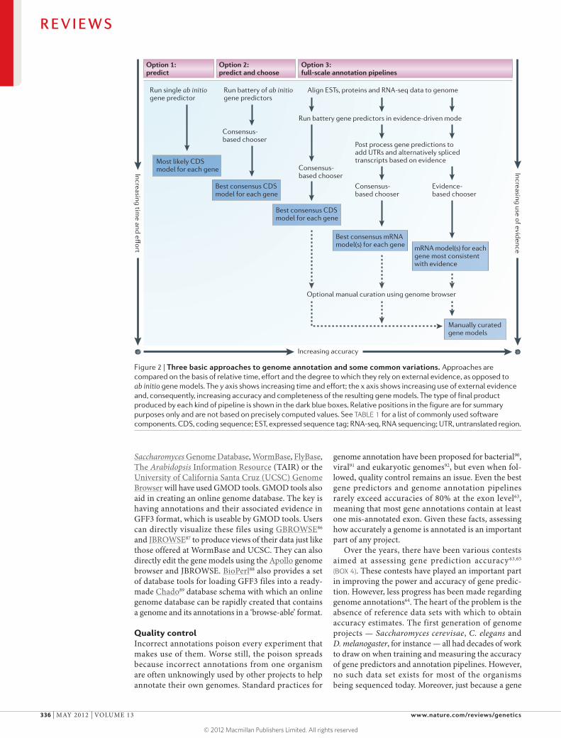
There are almost as many strategies for creating automated annotations as there are annotation pipe-lines, but the common theme is to use evidence to improve the accuracy of gene models, usually through some combination of pre- and post-processing of the gene predictions. FIGURE 2 and TABLE 1 provide an over-view of some of the more commonly used approaches.

Automated annotation. The simplest form of auto-mated annotation is to run a battery of different gene finders on the genome and then to use a ‘chooser algorithm’ (also known as a ‘combiner’) to select the single prediction whose intron–exon structure best represents the consensus of the models from among the overlapping predictions that define each putative gene locus. This is the process used by JIGSAW78. EVidenceModeler (EVM)79 and GLEAN80 (and its successor, Evigan81) go one step further, attempting to choose the best possible set of exons automatically and to combine them to produce annotations. This is done by estimating the types and frequencies of errors that are made by each source of gene evidence and then choosing combinations of evidence that minimize such errors. Like ab initio gene predictors, JIGSAW must be retrained for each new genome, and so it requires a source of known gene models that were not already used to train the underlying ab initio gene predictors. EVM allows the user to set expected evidence error rates manually or to learn them from a training set. By con-trast, GLEAN and Evigan use an unsupervised learning method to estimate a joint error model, and thus they require no additional training. In a recent gene pre-diction competition64, the combiners nearly always improved on the underlying gene prediction models, and JIGSAW, EVM or Evigan performed similarly.

Another popular approach is to feed the align-ment evidence to the gene predictors at run time (that is, evidence-driven prediction) to improve the accuracy of the prediction process — a chooser can then be used to identify the most representative prediction. The pre-dictions can also be processed — before or after running the chooser — to attain still greater accuracies by hav-ing the annotation pipeline add UTRs as suggested by the RNA-seq and EST data. This is the process used by PASA56,82, Gnomon73 and MAKER10. The evidence can also be used to inform the choices made by the chooser algorithm — by picking the post-processed gene model that is most consistent with the protein, EST and RNA-seq alignments83; EVM, MAKER and PASA all provide methods for doing so (TABLE 1; FIG. 2).

So which approach should you use? Probably the best way to think about the problem is in terms of effort versus accuracy. Simply running a single ab initio gene finder over even a very large genome can be done in a few hours of central processing unit (CPU) time. By contrast, a full run by an annotation pipeline such as MAKER or PASA can take weeks, but because these pipelines align evidence to the genome, their outputs provide starting points for annotation curation and downstream analyses, such as differential expres-sion analyses using RNA-seq data. Another factor to consider is the phylogenetic relationship of the study genome to other annotated genomes. If it is the first of its taxonomic order or family to be annotated, it would definitely be preferable to use a pipeline that can use the full repertory of external evidence, especially RNA-seq data, to inform its gene annotations; not doing so will almost certainly result in low-quality annotations80.

Visualizing the annotation data Output data: the importance of using a fully docu-mented format. The outputs of a genome annota-tion pipeline will include the transcript and protein sequences of every annotation, which are almost always provided in FASTA format84. Although FASTA files are useful, they only enable a small subset of pos-sible downstream analyses. Visualizing annotations in a genome browser and creating a genome database requires a more descriptive output file. At a bare mini-mum, output files need to describe the intron–exon structures of each annotation, their start and stop codons, UTRs and alternative transcripts. Ideally, these outputs should go one step further and should include information about the sequence alignments and gene predictions that support each gene model.

Four commonly used formats for describing annota-tions are the GenBank, GFF3, GTF and EMBL formats. Using a fully documented format is important for three reasons. First, doing so will remove the trouble of writ-ing software to convert outputs into a format that other tools can use. Second, common formats, especially those such as GenBank and GFF3, which use controlled vocabularies and ontologies to define their descriptive terminologies, guarantee ‘interoperability’ between analysis tools. Third, unless a common vocabulary is used to describe gene models85, comparative genomic analyses can be frustratingly difficult or downright impossible. In response to these needs, the Generic Model Organism Database (GMOD) project commu-nity has developed a series of standards and tools for description, analyses, visualization and redistribution of genome annotations, all of which use the GFF3 file format as inputs and outputs. Leveraging GMOD tools and GFF3 substantially simplifies curation, analysis, publication and management of genome annotations.

GMOD. The GMOD project is an umbrella organiza-tion that provides a large suite of tools for creating, managing and using genome annotations, includ-ing the analysis, visualization and redistribution of annotation data. Users who have browsed the

R E V I E W S

NATURE REVIEWS | GENETICS VOLUME 13 | MAY 2012 | 335

© 2012 Macmillan Publishers Limited. All rights reserved

Nature Reviews | Genetics

Post process gene predictions to add UTRs and alternatively splicedtranscripts based on evidence

Consensus-based chooser

Consensus-based chooser

Run battery of ab initiogene predictors

Align ESTs, proteins and RNA-seq data to genome

Run battery gene predictors in evidence-driven mode

Run single ab initiogene predictor

Best consensus CDSmodel for each gene

Best consensus mRNAmodel(s) for each gene mRNA model(s) for each

gene most consistent with evidence

Most likely CDSmodel for each gene

Optional manual curation using genome browser

Manually curatedgene models

Increasing accuracy

Consensus-based chooser

Evidence-based chooser

Best consensus CDSmodel for each gene

Option 2:predict and choose

Option 3:full-scale annotation pipelines

Option 1:predict

Increasing time and eff

ort

Increasing use of evidence

Figure 2 | Three basic approaches to genome annotation and some common variations. Approaches are compared on the basis of relative time, effort and the degree to which they rely on external evidence, as opposed to ab initio gene models. The y axis shows increasing time and effort; the x axis shows increasing use of external evidence and, consequently, increasing accuracy and completeness of the resulting gene models. The type of final product produced by each kind of pipeline is shown in the dark blue boxes. Relative positions in the figure are for summary purposes only and are not based on precisely computed values. See TABLE 1 for a list of commonly used software components. CDS, coding sequence; EST, expressed sequence tag; RNA-seq, RNA sequencing; UTR, untranslated region.

Saccharomyces Genome Database, WormBase, FlyBase, The Arabidopsis Information Resource (TAIR) or the University of California Santa Cruz (UCSC) Genome Browser will have used GMOD tools. GMOD tools also aid in creating an online genome database. The key is having annotations and their associated evidence in GFF3 format, which is useable by GMOD tools. Users can directly visualize these files using GBROWSE86 and JBROWSE87 to produce views of their data just like those offered at WormBase and UCSC. They can also directly edit the gene models using the Apollo genome browser and JBROWSE. BioPerl88 also provides a set of database tools for loading GFF3 files into a ready-made Chado89 database schema with which an online genome database can be rapidly created that contains a genome and its annotations in a ‘browse-able’ format.

Quality controlIncorrect annotations poison every experiment that makes use of them. Worse still, the poison spreads because incorrect annotations from one organism are often unknowingly used by other projects to help annotate their own genomes. Standard practices for

genome annotation have been proposed for bacterial90, viral91 and eukaryotic genomes92, but even when fol-lowed, quality control remains an issue. Even the best gene predictors and genome annotation pipelines rarely exceed accuracies of 80% at the exon level63, meaning that most gene annotations contain at least one mis-annotated exon. Given these facts, assessing how accurately a genome is annotated is an important part of any project.

Over the years, there have been various contests aimed at assessing gene prediction accuracy 63,65 (BOX 4). These contests have played an important part in improving the power and accuracy of gene predic-tion. However, less progress has been made regarding genome annotations64. The heart of the problem is the absence of reference data sets with which to obtain accuracy estimates. The first generation of genome projects — Saccharomyces cerevisae, C. elegans and D. melanogaster, for instance — all had decades of work to draw on when training and measuring the accuracy of gene predictors and annotation pipelines. However, no such data set exists for most of the organisms being sequenced today. Moreover, just because a gene

R E V I E W S

336 | MAY 2012 | VOLUME 13 www.nature.com/reviews/genetics

© 2012 Macmillan Publishers Limited. All rights reserved

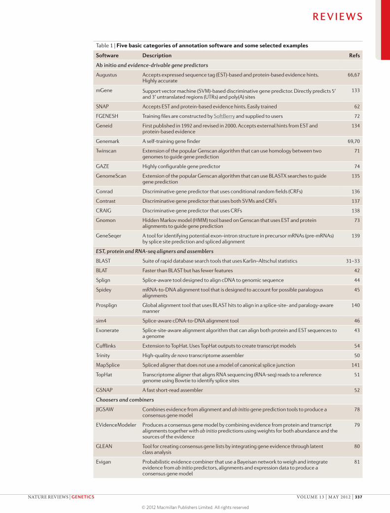
Table 1 | Five basic categories of annotation software and some selected examples

Software Description Refs

Ab initio and evidence-drivable gene predictors

Augustus Accepts expressed sequence tag (EST)-based and protein-based evidence hints. Highly accurate

66,67

mGene Support vector machine (SVM)-based discriminative gene predictor. Directly predicts 5′ and 3′ untranslated regions (UTRs) and poly(A) sites

133

SNAP Accepts EST and protein-based evidence hints. Easily trained 62

FGENESH Training files are constructed by SoftBerry and supplied to users 72

Geneid First published in 1992 and revised in 2000. Accepts external hints from EST and protein-based evidence

134

Genemark A self-training gene finder 69,70

Twinscan Extension of the popular Genscan algorithm that can use homology between two genomes to guide gene prediction

71

GAZE Highly configurable gene predictor 74

GenomeScan Extension of the popular Genscan algorithm that can use BLASTX searches to guide gene prediction

135

Conrad Discriminative gene predictor that uses conditional random fields (CRFs) 136

Contrast Discriminative gene predictor that uses both SVMs and CRFs 137

CRAIG Discriminative gene predictor that uses CRFs 138

Gnomon Hidden Markov model (HMM) tool based on Genscan that uses EST and protein alignments to guide gene prediction

73

GeneSeqer A tool for identifying potential exon–intron structure in precursor mRNAs (pre-mRNAs) by splice site prediction and spliced alignment

139

EST, protein and RNA-seq aligners and assemblers

BLAST Suite of rapid database search tools that uses Karlin–Altschul statistics 31–33

BLAT Faster than BLAST but has fewer features 42

Splign Splice-aware tool designed to align cDNA to genomic sequence 44

Spidey mRNA-to-DNA alignment tool that is designed to account for possible paralogous alignments

45

Prosplign Global alignment tool that uses BLAST hits to align in a splice-site- and paralogy-aware manner

140

sim4 Splice-aware cDNA-to-DNA alignment tool 46

Exonerate Splice-site-aware alignment algorithm that can align both protein and EST sequences to a genome

43

Cufflinks Extension to TopHat. Uses TopHat outputs to create transcript models 54

Trinity High-quality de novo transcriptome assembler 50

MapSplice Spliced aligner that does not use a model of canonical splice junction 141

TopHat Transcriptome aligner that aligns RNA sequencing (RNA-seq) reads to a reference genome using Bowtie to identify splice sites

51

GSNAP A fast short-read assembler 52

Choosers and combiners

JIGSAW Combines evidence from alignment and ab initio gene prediction tools to produce a consensus gene model

78

EVidenceModeler Produces a consensus gene model by combining evidence from protein and transcript alignments together with ab initio predictions using weights for both abundance and the sources of the evidence

79

GLEAN Tool for creating consensus gene lists by integrating gene evidence through latent class analysis

80

Evigan Probabilistic evidence combiner that use a Bayeisan network to weigh and integrate evidence from ab initio predictors, alignments and expression data to produce a consensus gene model

81

R E V I E W S

NATURE REVIEWS | GENETICS VOLUME 13 | MAY 2012 | 337

© 2012 Macmillan Publishers Limited. All rights reserved

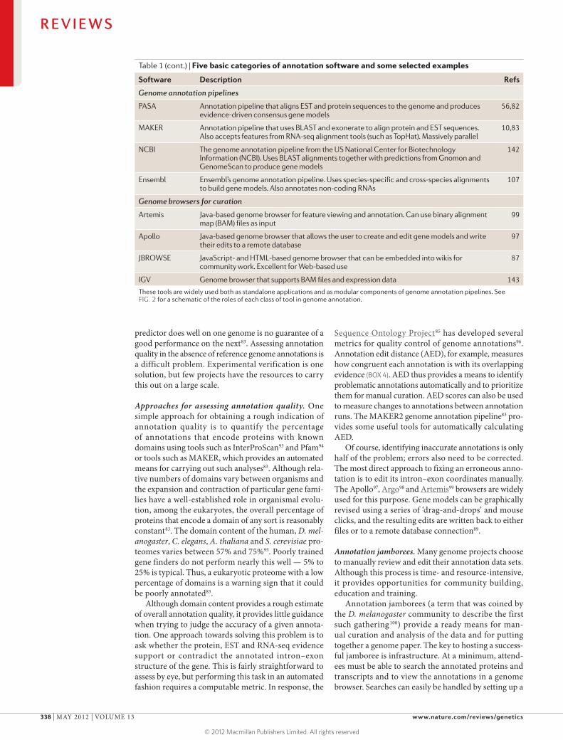
Table 1 (cont.) | Five basic categories of annotation software and some selected examples

Software Description Refs

Genome annotation pipelines

PASA Annotation pipeline that aligns EST and protein sequences to the genome and produces evidence-driven consensus gene models

56,82

MAKER Annotation pipeline that uses BLAST and exonerate to align protein and EST sequences. Also accepts features from RNA-seq alignment tools (such as TopHat). Massively parallel

10,83

NCBI The genome annotation pipeline from the US National Center for Biotechnology Information (NCBI). Uses BLAST alignments together with predictions from Gnomon and GenomeScan to produce gene models

142

Ensembl Ensembl’s genome annotation pipeline. Uses species-specific and cross-species alignments to build gene models. Also annotates non-coding RNAs

107

Genome browsers for curation

Artemis Java-based genome browser for feature viewing and annotation. Can use binary alignment map (BAM) files as input

99

Apollo Java-based genome browser that allows the user to create and edit gene models and write their edits to a remote database

97

JBROWSE JavaScript- and HTML-based genome browser that can be embedded into wikis for community work. Excellent for Web-based use

87

IGV Genome browser that supports BAM files and expression data 143

These tools are widely used both as standalone applications and as modular components of genome annotation pipelines. See FIG. 2 for a schematic of the roles of each class of tool in genome annotation.

predictor does well on one genome is no guarantee of a good performance on the next83. Assessing annotation quality in the absence of reference genome annotations is a difficult problem. Experimental verification is one solution, but few projects have the resources to carry this out on a large scale.

Approaches for assessing annotation quality. One simple approach for obtaining a rough indication of annotation quality is to quantify the percentage of annotations that encode proteins with known domains using tools such as InterProScan93 and Pfam94 or tools such as MAKER, which provides an automated means for carrying out such analyses83. Although rela-tive numbers of domains vary between organisms and the expansion and contraction of particular gene fami-lies have a well-established role in organismal evolu-tion, among the eukaryotes, the overall percentage of proteins that encode a domain of any sort is reasonably constant83. The domain content of the human, D. mel-anogaster, C. elegans, A. thaliana and S. cerevisiae pro-teomes varies between 57% and 75%95. Poorly trained gene finders do not perform nearly this well — 5% to 25% is typical. Thus, a eukaryotic proteome with a low percentage of domains is a warning sign that it could be poorly annotated83.

Although domain content provides a rough estimate of overall annotation quality, it provides little guidance when trying to judge the accuracy of a given annota-tion. One approach towards solving this problem is to ask whether the protein, EST and RNA-seq evidence support or contradict the annotated intron–exon structure of the gene. This is fairly straightforward to assess by eye, but performing this task in an automated fashion requires a computable metric. In response, the

Sequence Ontology Project85 has developed several metrics for quality control of genome annotations96. Annotation edit distance (AED), for example, measures how congruent each annotation is with its overlapping evidence (BOX 4). AED thus provides a means to identify problematic annotations automatically and to prioritize them for manual curation. AED scores can also be used to measure changes to annotations between annotation runs. The MAKER2 genome annotation pipeline83 pro-vides some useful tools for automatically calculating AED.

Of course, identifying inaccurate annotations is only half of the problem; errors also need to be corrected. The most direct approach to fixing an erroneous anno-tation is to edit its intron–exon coordinates manually. The Apollo97, Argo98 and Artemis99 browsers are widely used for this purpose. Gene models can be graphically revised using a series of ‘drag-and-drops’ and mouse clicks, and the resulting edits are written back to either files or to a remote database connection89.

Annotation jamborees. Many genome projects choose to manually review and edit their annotation data sets. Although this process is time- and resource-intensive, it provides opportunities for community building, education and training.

Annotation jamborees (a term that was coined by the D. melanogaster community to describe the first such gathering100) provide a ready means for man-ual curation and analysis of the data and for putting together a genome paper. The key to hosting a success-ful jamboree is infrastructure. At a minimum, attend-ees must be able to search the annotated proteins and transcripts and to view the annotations in a genome browser. Searches can easily be handled by setting up a

R E V I E W S

338 | MAY 2012 | VOLUME 13 www.nature.com/reviews/genetics

© 2012 Macmillan Publishers Limited. All rights reserved

BLAST database server coupled with a graphical user interface (GUI) such as a Web browser. The WWW BLAST server package101 provides an easy means to do so. GBrowse86,102 and JBrowse87 can also easily be con-figured to allow remote users to view the annotated genome, as can the Apollo genome browser, which also provides a means to edit incorrect annotations. As all of these resources can be set up and configured remotely, it is now possible to support a distributed jamboree, in which the community collaborates via the Internet. This model recently proved to be successful for the ant genome community, which organized a distributed jamboree in which investigators and students collabo-rated to curate and analyse three different ant genomes quickly, all in a distributed manner103–106.

Making data publicly available Successful genome annotation projects do not just end with the publication of a paper; they also produce pub-licly available annotations. Genome annotations fuel the bench work and computational analyses that con-stitute the day-to-day operations of molecular biology and bioinformatics laboratories worldwide. They also provide an essential resource for other genome anno-tation projects; the transcripts and proteins produced by one annotation project will probably be used to help annotate other genomes. There are three basic routes to making annotations publicly available: you can build your own genome database and place it online; you can submit your annotations to GenBank and Ensembl; or you can submit them to any of a growing number of theme-based genome databases. We recommend taking all three routes.

Submitting annotations to public databases. One way to make annotations publicly available is to submit them to GenBank. Parties working on vertebrate genomes are also encouraged to contact Ensembl, which con-tinues to incorporate new species at the rate of 5–10 per year in order to create a comprehensive annotation resource for vertebrate genomes, all of which are anno-tated by its gene build pipeline107. Both GenBank and Ensembl have much to offer to smaller genome pro-jects, including powerful data-marts that allow users to browse and download data. Ensembl and GenBank also automatically handle the heavy lifting that is involved in relating gene models to those of other organisms and identifying homologues, paralogues and orthologues. They also provide an easy means to search and browse data; in short, they integrate a data set into the larger landscape of genomics and genome annotations. Best of all, the entire process is free, and submission to these sites in no way abridges the rights of the generators of the data to host and maintain their own genome data-base. For the research communities of most organisms, members will prefer to visit the specialized genome database for that organism, whereas the larger biologi-cal community will tend to access the data through GenBank and Ensembl. In addition to these large sites, intermediate-sized projects that host, manage and maintain sets of annotated genomes that are all

related by a common theme are gaining in popularity. Examples include BeeBase103, Gramene108, PlantGDB109, Phytozome110 and VectorBase111.

Updating annotations. Many genomes were annotated so long ago that the existing annotations could be dra-matically improved using modern tools and data sets such as RNA-seq. In many cases, improved assemblies are possible as well. The question then becomes how to merge, update and improve the existing annotations and, at the same time, to document the process. Like annotation quality control, this is a thorny problem that until recently has garnered little attention, and few published tools yet exist to automate the pro-cess. Among existing tools, GLEAN and PASA can be used to report differences between pre-existing gene models and newly created ones. Ensembl has a proce-dure to merge annotation data sets to produce a con-sensus, and PASA has one for updating annotations with RNA-seq data. The MAKER annotation pipeline provides an automated toolkit with all of these func-tionalities and can revise, update and merge existing annotation data sets, as well as map them forwards to new assemblies10,83.

GenBank provides two avenues for redistributing the results of updates and re-annotation of genomes. If the group that is updating the annotations includes the original authors, the update can simply be submit-ted; if not, there are two routes for submission. If the work involves substantial improvements to the original assembly, the parties producing them can submit the new annotations to GenBank as primary authors; if not — that is, if the revisions merely improve the original annotations — those producing them can submit their work through the third party submission channel. Ensembl also allows submission of such data, although the process is less formal, and interested parties should contact Ensembl directly.

ConclusionsIn some ways, cheap sequencing has complicated genome annotation. As we have explained, the frag-mented assemblies and exotic nature of many of the cur-rent genome-sequencing projects are part of the reason that this is so, but it is the ever-widening scope of annotation that is presenting the greatest challenges. Genome annotation has moved beyond merely identi-fying protein-coding genes to include an ever-greater emphasis on the annotation of transposons, regula-tory regions, pseudogenes and ncRNA genes112–115. Annotation quality control and management are also increasingly becoming bottlenecks. As long as tools and sequencing technologies continue to develop, periodic updates to every genome’s annotations will remain nec-essary. Those undertaking genome annotation projects need to reflect on this fact. Like parenthood, annota-tion responsibilities do not end with birth. Incorrect and incomplete annotations poison every experi-ment that makes use of them. In today’s genomics- driven world, providing accurate and up-to-date annotations is simply a must.

Data-mart Provides users with online access to the contents of a data warehouse through user-configurable queries. A data-mart allows users to download data that meet their particular needs: for example, all transcripts from all annotated genes on human chromosome 3.

R E V I E W S

NATURE REVIEWS | GENETICS VOLUME 13 | MAY 2012 | 339

© 2012 Macmillan Publishers Limited. All rights reserved

1. Adams, M. D. et al. The genome sequence of Drosophila melanogaster. Science 287, 2185–2195 (2000).

2. Celniker, S. E. et al. Finishing a whole-genome shotgun: release 3 of the Drosophila melanogaster euchromatic genome sequence. Genome Biol. 3, research0079 (2002).

3. Venter, J. C. et al. The sequence of the human genome. Science 291, 1304–1351 (2001).

4. Finishing the euchromatic sequence of the human genome. Nature 431, 931–945 (2004).

5. Denoeud, F. et al. Annotating genomes with massive-scale RNA sequencing. Genome Biol. 9, R175 (2008).

6. Ozsolak, F. et al. Direct RNA sequencing. Nature 461, 814–818 (2009).

7. Mortazavi, A., Williams, B. A., McCue, K., Schaeffer, L. & Wold, B. Mapping and quantifying mammalian transcriptomes by RNA-seq. Nature Methods 5, 621–628 (2008).

8. Wang, E. T. et al. Alternative isoform regulation in human tissue transcriptomes. Nature 456, 470–476 (2008).This paper provides one of the most extensively documented surveys of alternatively spliced transcripts. It is a key publication for understanding how extensive alternative splicing is in human tissues, for understanding how powerful RNA-seq data are as a tool for discovering new transcripts and for quantifying their abundance and differential expression patterns.

9. Chain, P. S. et al. Genomics. Genome project standards in a new era of sequencing. Science 326, 236–237 (2009).

10. Cantarel, B. L. et al. MAKER: an easy-to-use annotation pipeline designed for emerging model organism genomes. Genome Res. 18, 188–196 (2008).

11. Ye, L. et al. A vertebrate case study of the quality of assemblies derived from next-generation sequences. Genome Biol. 12, R31 (2011).

12. Parra, G., Bradnam, K. & Korf, I. CEGMA: a pipeline to accurately annotate core genes in eukaryotic genomes. Bioinformatics 23, 1061–1067 (2007).

13. Tsai, I. J., Otto, T. D. & Berriman, M. Improving draft assemblies by iterative mapping and assembly of short reads to eliminate gaps. Genome Biol. 11, R41 (2010).

14. Assefa, S., Keane, T. M., Otto, T. D., Newbold, C. & Berriman, M. ABACAS: algorithm-based automatic contiguation of assembled sequences. Bioinformatics 25, 1968–1969 (2009).

15. Husemann, P. & Stoye, J. r2cat: synteny plots and comparative assembly. Bioinformatics 26, 570–571 (2010).

16. Kapitonov, V. V. & Jurka, J. A novel class of SINE elements derived from 5S rRNA. Mol. Biol. Evol. 20, 694–702 (2003).

17. Kapitonov, V. V. & Jurka, J. A universal classification of eukaryotic transposable elements implemented in Repbase. Nature Rev. Genet. 9, 411–412; author reply 414 (2008).

18. Lander, E. S. et al. Initial sequencing and analysis of the human genome. Nature 409, 860–921 (2001).

19. Buisine, N., Quesneville, H. & Colot, V. Improved detection and annotation of transposable elements in sequenced genomes using multiple reference sequence sets. Genomics 91, 467–475 (2008).

20. Han, Y. & Wessler, S. R. MITE-Hunter: a program for discovering miniature inverted-repeat transposable elements from genomic sequences. Nucleic Acids Res. 38, e199 (2010).

21. McClure, M. A. et al. Automated characterization of potentially active retroid agents in the human genome. Genomics 85, 512–523 (2005).

22. Bao, Z. & Eddy, S. R. Automated de novo identification of repeat sequence families in sequenced genomes. Genome Res. 12, 1269–1276 (2002).

23. Price, A. L., Jones, N. C. & Pevzner, P. A. De novo identification of repeat families in large genomes. Bioinformatics 21 (Suppl. 1), i351–i358 (2005).

24. Smit, A. & Hubley, R. RepeatModeler 1.05. repeatmasker.org [online], http://www.repeatmasker.org/RepeatModeler.html (2011).

25. Morgulis, A., Gertz, E. M., Schaffer, A. A. & Agarwala, R. WindowMasker: window-based masker for sequenced genomes. Bioinformatics 22, 134–141 (2006).

26. Treangen, T. J. & Salzberg, S. L. Repetitive DNA and next-generation sequencing: computational challenges and solutions. Nature Rev. Genet. 13, 36–46 (2012).

27. Bergman, C. M. & Quesneville, H. Discovering and detecting transposable elements in genome sequences. Brief. Bioinform. 8, 382–392 (2007).

28. Cordaux, R. & Batzer, M. A. The impact of retrotransposons on human genome evolution. Nature Rev. Genet. 10, 691–703 (2009).

29. Witherspoon, D. J. et al. Alu repeats increase local recombination rates. BMC Genomics 10, 530 (2009).

30. Smit, A. F., Hubley, R. & Green, P. RepeatMasker 3.0 repeatmasker.org [online], http://www.repeatmasker.org/webrepeatmaskerhelp.html (1996–2010).

31. Altschul, S. F., Gish, W., Miller, W., Myers, E. W. & Lipman, D. J. Basic local alignment search tool. J. Mol. Biol. 215, 403–410 (1990).

32. Korf, I., Yandell, M. & Bedell, J. BLAST: an Essential Guide to the Basic Local Alignment Search Tool 339 (O’Reilly & Associates, 2003).Everyone involved with a genome project should be familiar with BLAST. Reference 31 is the original paper describing this tool. Reference 32 is an entire book describing BLAST and how it is used.

33. Altschul, S. F. et al. Gapped BLAST and PSI-BLAST: a new generation of protein database search programs. Nucleic Acids Res. 25, 3389–3402 (1997).

34. Green, P. Crossmatch. A general purpose utility for comparing any two sets of DNA sequences. PHRAP [online], http://www.phrap.org/phredphrap/general.html (1993–1996).

35. Majoros, W. H. Methods for Computational Gene Prediction 2 (Cambridge Univ. Press, 2007).

36. Camacho, C. et al. BLAST+: architecture and applications. BMC Bioinformatics 10, 421 (2009).

37. Bairoch, A., Boeckmann, B., Ferro, S. & Gasteiger, E. Swiss-Prot: juggling between evolution and stability. Brief. Bioinform. 5, 39–55 (2004).

38. Boeckmann, B. et al. Protein variety and functional diversity: Swiss-Prot annotation in its biological context. C.R. Biol. 328, 882–899 (2005).

39. The UniProt Consortium. Ongoing and future developments at the Universal Protein Resource. Nucleic Acids Res. 39, D214–D219 (2011).

40. Benson, D. A., Karsch-Mizrachi, I., Lipman, D. J., Ostell, J. & Sayers, E. W. GenBank. Nucleic Acids Res. 37, D26–D31 (2009).

41. Sayers, E. W. et al. Database resources of the National Center for Biotechnology Information. Nucleic Acids Res. 37, D5–D15 (2009).

42. Kent, W. J. BLAT—the BLAST-like alignment tool. Genome Res. 12, 656–664 (2002).

43. Slater, G. S. & Birney, E. Automated generation of heuristics for biological sequence comparison. BMC Bioinformatics 6, 31 (2005).

44. Kapustin, Y., Souvorov, A., Tatusova, T. & Lipman, D. Splign: algorithms for computing spliced alignments with identification of paralogs. Biol. Direct 3, 20 (2008).

45. Wheelan, S. J., Church, D. M. & Ostell, J. M. Spidey: a tool for mRNA-to-genomic alignments. Genome Res. 11, 1952–1957 (2001).

46. Florea, L., Hartzell, G., Zhang, Z., Rubin, G. M. & Miller, W. A computer program for aligning a cDNA sequence with a genomic DNA sequence. Genome Res. 8, 967–974 (1998).

47. Garber, M., Grabherr, M. G., Guttman, M. & Trapnell, C. Computational methods for transcriptome annotation and quantification using RNA-seq. Nature Methods 8, 469–477 (2011).

48. Simpson, J. T. et al. ABySS: a parallel assembler for short read sequence data. Genome Res. 19, 1117–1123 (2009).

49. Li, R. et al. De novo assembly of human genomes with massively parallel short read sequencing. Genome Res. 20, 265–272 (2010).

50. Grabherr, M. G. et al. Full-length transcriptome assembly from RNA-seq data without a reference genome. Nature Biotech. 29, 644–652 (2011).This paper describes Trinity, a transcriptome assembler that was specifically designed for next-generation sequence data. It is required reading for anyone trying to use RNA-seq data for genome annotation.

51. Trapnell, C., Pachter, L. & Salzberg, S. L. TopHat: discovering splice junctions with RNA-seq. Bioinformatics 25, 1105–1111 (2009).

52. Wu, T. D. & Nacu, S. Fast and SNP-tolerant detection of complex variants and splicing in short reads. Bioinformatics 26, 873–881 (2010).

53. Guttman, M. et al. Ab initio reconstruction of cell type-specific transcriptomes in mouse reveals the conserved multi-exonic structure of lincRNAs. Nature Biotech. 28, 503–510 (2010).

54. Trapnell, C. et al. Transcript assembly and quantification by RNA-seq reveals unannotated transcripts and isoform switching during cell differentiation. Nature Biotech. 28, 511–515 (2010).

55. Trapnell, C. et al. Differential gene and transcript expression analysis of RNA-seq experiments with TopHat and Cufflinks. Nature Protoc. 7, 562–578 (2012).This paper describes best practice approaches for combining TopHat and Cufflinks when using RNA-seq data for genome annotation.

56. Haas, B. J. et al. Improving the Arabidopsis genome annotation using maximal transcript alignment assemblies. Nucleic Acids Res. 31, 5654–5666 (2003).

57. Guigo, R., Knudsen, S., Drake, N. & Smith, T. Prediction of gene structure. J. Mol. Biol. 226, 141–157 (1992).

58. Solovyev, V. V., Salamov, A. A. & Lawrence, C. B. The prediction of human exons by oligonucleotide composition and discriminant analysis of spliceable open reading frames. Proc. Int. Conf. Intell. Syst. Mol. Biol. 2, 354–362 (1994).

59. Burge, C. & Karlin, S. Prediction of complete gene structures in human genomic DNA. J. Mol. Biol. 268, 78–94 (1997).This study describes the ab initio gene predictor GenScan. It is a classic paper that is full of informative explanations of the problems associated with eukaryotic gene prediction.

60. Reese, M. G., Kulp, D., Tammana, H. & Haussler, D. Genie—gene finding in Drosophila melanogaster. Genome Res. 10, 529–538 (2000).

61. Brent, M. R. Genome annotation past, present, and future: how to define an ORF at each locus. Genome Res. 15, 1777–1786 (2005).

62. Korf, I. Gene finding in novel genomes. BMC Bioinformatics 5, 59 (2004).This paper describes a gene predictor, SNAP, that is easy to use and to configure. It also clearly explains the pitfalls that are associated with using a poorly trained gene finder or one that has been trained on a different genome from the one that is being annotated.

63. Reese, M. G. & Guigo, R. EGASP: Introduction. Genome Biol. 7 (Suppl. 1), 1–3 (2006).This is the introduction to an entire issue of Genome Biology that is dedicated to benchmarking an entire host of eukaryotic gene finders and annotation pipelines. Anyone involved with a genome annotation project should have a look at every paper in this special supplement.

64. Coghlan, A. et al. nGASP—the nematode genome annotation assessment project. BMC Bioinformatics 9, 549 (2008).

65. Guigo, R. & Reese, M. G. EGASP: collaboration through competition to find human genes. Nature Methods 2, 575–577 (2005).

66. Stanke, M. & Waack, S. Gene prediction with a hidden Markov model and a new intron submodel. Bioinformatics 19 (Suppl. 2), ii215–ii225 (2003).

67. Stanke, M., Schoffmann, O., Morgenstern, B. & Waack, S. Gene prediction in eukaryotes with a generalized hidden Markov model that uses hints from external sources. BMC Bioinformatics 7, 62 (2006).

68. Lukashin, A. V. & Borodovsky, M. GeneMark.hmm: new solutions for gene finding. Nucleic Acids Res. 26, 1107–1115 (1998).

69. Ter-Hovhannisyan, V., Lomsadze, A., Chernoff, Y. O. & Borodovsky, M. Gene prediction in novel fungal genomes using an ab initio algorithm with unsupervised training. Genome Res. 18, 1979–1990 (2008).

70. Zhu, W., Lomsadze, A. & Borodovsky, M. Ab initio gene identification in metagenomic sequences. Nucleic Acids Res. 38, e132 (2010).

71. Korf, I., Flicek, P., Duan, D. & Brent, M. R. Integrating genomic homology into gene structure prediction. Bioinformatics 17, S140–S148 (2001).

72. Salamov, A. A. & Solovyev, V. V. Ab initio gene finding in Drosophila genomic DNA. Genome Res. 10, 516–522 (2000).

73. Souvorov, A. et al. Gnomon — the NCBI eukaryotic gene prediction tool. National Center for Biotechnology Information [online], http://www.ncbi.nlm.nih.gov/genome/guide/gnomon.shtml (2010).

R E V I E W S

340 | MAY 2012 | VOLUME 13 www.nature.com/reviews/genetics

© 2012 Macmillan Publishers Limited. All rights reserved

74. Howe, K. L., Chothia, T. & Durbin, R. GAZE: a generic framework for the integration of gene-prediction data by dynamic programming. Genome Res. 12, 1418–1427 (2002).

75. Mungall, C. J. et al. An integrated computational pipeline and database to support whole-genome sequence annotation. Genome Biol. 3, research0081 (2002).

76. Misra, S. et al. Annotation of the Drosophila melanogaster euchromatic genome: a systematic review. Genome Biol. 3, research0083 (2002).

77. Yandell, M. et al. A computational and experimental approach to validating annotations and gene predictions in the Drosophila melanogaster genome. Proc. Natl Acad. Sci. USA 102, 1566–1571 (2005).

78. Allen, J. E. & Salzberg, S. L. JIGSAW: integration of multiple sources of evidence for gene prediction. Bioinformatics 21, 3596–3603 (2005).

79. Haas, B. J. et al. Automated eukaryotic gene structure annotation using EVidenceModeler and the Program to Assemble Spliced Alignments. Genome Biol. 9, R7 (2008).

80. Elsik, C. G. et al. Creating a honey bee consensus gene set. Genome Biol. 8, R13 (2007).

81. Liu, Q., Mackey, A. J., Roos, D. S. & Pereira, F. C. Evigan: a hidden variable model for integrating gene evidence for eukaryotic gene prediction. Bioinformatics 24, 597–605 (2008).

82. Haas, B. J., Zeng, Q., Pearson, M. D., Cuomo, C. A. & Wortman, J. R. Approaches to fungal genome annotation. Mycology 2, 118–141 (2011).This paper provides an excellent description of the process used by the Broad Institute for fungal annotation. It is also a good resource for those seeking to learn more about PASA; for more information about PASA, see reference 56.

83. Holt, C. & Yandell, M. MAKER2: an annotation pipeline and genome-database management tool for second-generation genome projects. BMC Bioinformatics 12, 491 (2011).This study describes the database management and annotation quality-control tools for the MAKER2 genome annotation pipeline. It also explains many of the challenges that are associated with annotating novel genomes and how to overcome them.

84. Pearson, W. R. & Lipman, D. J. Improved tools for biological sequence comparison. Proc. Natl Acad. Sci. USA 85, 2444–2448 (1988).

85. Eilbeck, K. et al. The Sequence Ontology: a tool for the unification of genome annotations. Genome Biol. 6, R44 (2005).

86. Donlin, M. J. in Current Protocols in Bioinformatics. Ch. 9, Unit 9.9 (2007).

87. Skinner, M. E., Uzilov, A. V., Stein, L. D., Mungall, C. J. & Holmes, I. H. JBrowse: a next-generation genome browser. Genome Res. 19, 1630–1638 (2009).

88. Stajich, J. E. et al. The Bioperl toolkit: Perl modules for the life sciences. Genome Res. 12, 1611–1618 (2002).

89. Zhou, P., Emmert, D. & Zhang, P. in Current Protocols in Bioinformatics Ch. 9, Unit 9.6 (2006).

90. Klimke, W. et al. Solving the problem: genome annotation standards before the data deluge. Stand. Genomic Sci. 5, 168–193 (2011).

91. Brister, J. R. et al. Towards viral genome annotation standards, report from the 2010 NCBI annotation workshop. Viruses 2, 2258–2268 (2010).

92. Madupu, R. et al. Meeting report: a workshop on best practices in genome annotation. Database 2010, baq001 (2010).

93. Mulder, N. & Apweiler, R. InterPro and InterProScan: tools for protein sequence classification and comparison. Methods Mol. Biol. 396, 59–70 (2007).

94. Finn, R. D. et al. The Pfam protein families database. Nucleic Acids Res. 38, D211–D222 (2010).

95. Holt, C. Tools and Techniques for Genome Annotation Analysis. Ph.D. thesis, Univ. Utah (2011).

96. Eilbeck, K., Moore, B., Holt, C. & Yandell, M. Quantitative measures for the management and comparison of annotated genomes. BMC Bioinformatics 10, 67 (2009).This paper describes a number of annotation quality- control measures, including annotation edit distance (AED). It also provides some interesting meta-analyses describing the impact of curation efforts on the gene annotations of several model organism databases over a period of several years.

97. Lewis, S. E. et al. Apollo: a sequence annotation editor. Genome Biol. 3, research0082 (2002).

98. Engels, R. Argo Genome Browser version 1.0.31. Broad Institute [online], http://www.broadinstitute.org/annotation/argo (2010).

99. Rutherford, K. et al. Artemis: sequence visualization and annotation. Bioinformatics 16, 944–945 (2000).

100. Hartl, D. L. Fly meets shotgun: shotgun wins. Nature Genet. 24, 327–328 (2000).

101. Desk, B. H. Introduction to the standalone WWW Blast server. National Center for Biotechnology Information [online], http://www.ncbi.nlm.nih.gov/blast/docs/wwwblast.html (2002).This page explains how to use a suite of programs to set up a local Blast server for your local database.

102. Stein, L. D. et al. The generic genome browser: a building block for a model organism system database. Genome Res. 12, 1599–1610 (2002).

103. Munoz-Torres, M. C. et al. Hymenoptera Genome Database: integrated community resources for insect species of the order Hymenoptera. Nucleic Acids Res. 39, D658–D662 (2011).

104. Smith, C. D. et al. Draft genome of the globally widespread and invasive Argentine ant (Linepithema humile). Proc. Natl Acad. Sci. USA 108, 5673–5678 (2011).

105. Suen, G. et al. The genome sequence of the leaf-cutter ant Atta cephalotes reveals insights into its obligate symbiotic lifestyle. PLoS Genet. 7, e1002007 (2011).

106. Nygaard, S. et al. The genome of the leaf-cutting ant Acromyrmex echinatior suggests key adaptations to advanced social life and fungus farming. Genome Res. 21, 1339–1348 (2011).

107. Curwen, V. et al. The Ensembl automatic gene annotation system. Genome Res. 14, 942–950 (2004).This paper describes the Ensembl genome annotation pipeline; although the article is now several years old, it is still a good place to start. We would recommend reading this paper and then browsing the extensive Ensembl web site for more information.

108. Youens-Clark, K. et al. Gramene database in 2010: updates and extensions. Nucleic Acids Res. 39, D1085–D1094 (2011).

109. Duvick, J. et al. PlantGDB: a resource for comparative plant genomics. Nucleic Acids Res. 36, D959–D965 (2008).

110. Goodstein, D. M. et al. Phytozome: a comparative platform for green plant genomics. Nucleic Acids Res. 40, D1178–D1186 (2012).

111. Lawson, D. et al. VectorBase: a data resource for invertebrate vector genomics. Nucleic Acids Res. 37, D583–D587 (2009).

112. Karro, J. E. et al. Pseudogene.org: a comprehensive database and comparison platform for pseudogene annotation. Nucleic Acids Res. 35, D55–D60 (2007).

113. Zheng, D. et al. Integrated pseudogene annotation for human chromosome 22: evidence for transcription. J. Mol. Biol. 349, 27–45 (2005).

114. Griffiths-Jones, S., Bateman, A., Marshall, M., Khanna, A. & Eddy, S. R. Rfam: an RNA family database. Nucleic Acids Res. 31, 439–441 (2003).

115. Lagesen, K. et al. RNAmmer: consistent and rapid annotation of ribosomal RNA genes. Nucleic Acids Res. 35, 3100–3108 (2007).

116. Dolezel, J. & Bartos, J. Plant DNA flow cytometry and estimation of nuclear genome size. Ann. Botany 95, 99–110 (2005).

117. Laird, C. D. & McCarthy, B. J. Molecular characterization of the Drosophila genome. Genetics 63, 865–882 (1969).

118. Lowe, T. M. & Eddy, S. R. tRNAscan-SE: a program for improved detection of transfer RNA genes in genomic sequence. Nucleic Acids Res. 25, 955–964 (1997).

119. Schattner, P., Brooks, A. N. & Lowe, T. M. The tRNAscan-SE, snoscan and snoGPS web servers for the detection of tRNAs and snoRNAs. Nucleic Acids Res. 33, W686–W689 (2005).

120. Lewis, B. P., Shih, I. H., Jones-Rhoades, M. W., Bartel, D. P. & Burge, C. B. Prediction of mammalian microRNA targets. Cell 115, 787–798 (2003).

121. Eddy, S. R. A memory-efficient dynamic programming algorithm for optimal alignment of a sequence to an RNA secondary structure. BMC Bioinformatics 3, 18 (2002).

122. Holmes, I. & Rubin, G. M. Pairwise RNA structure comparison with stochastic context-free grammars. Pac. Symp. Biocomput. 7, 163–174 (2002).

123. QIAGEN. Quick-Start Protocol miRNAeasy Mini Kit. QIAGEN [online], http://www.qiagen.com/products/rnastabilizationpurification/microrna/mirneasyminikit.aspx#Tabs=t2 (2011).

124. Chen, C. et al. Real-time quantification of microRNAs by stem–loop RT-PCR. Nucleic Acids Res. 33, e179 (2005).

125. van Leeuwen, S. & Mikkers, H. Long non-coding RNAs: guardians of development. Differentiation 80, 175–183 (2010).

126. Hung., T. & Chang, H. Y. Long noncoding RNA in genome regulation: prospects and mechanisms. RNA Biol. 7, 582–585 (2010).

127. Tam, O. H. et al. Pseudogene-derived small interfering RNAs regulate gene expression in mouse oocytes. Nature 453, 534–538 (2008).

128. Zhang, Z., Carriero, N. & Gerstein, M. Comparative analysis of processed pseudogenes in the mouse and human genomes. Trends Genet. 20, 62–67 (2004).

129. Nawrocki, E. P., Kolbe, D. L. & Eddy, S. R. Infernal 1.0: inference of RNA alignments. Bioinformatics 25, 1335–1337 (2009).

130. Burset, M. & Guigo, R. Evaluation of gene structure prediction programs. Genomics 34, 353–367 (1996).This paper provides an excellent explanation of how sensitivity and specificity measures can be used to evaluate gene finder performance. This is a classic paper in the field and should be read by anyone involved in gene annotation.

131. Baldi, P., Brunak, S., Chauvin, Y., Andersen, C. A. & Nielsen, H. Assessing the accuracy of prediction algorithms for classification: an overview. Bioinformatics 16, 412–424 (2000).

132. Guigo, R. et al. EGASP: the human ENCODE Genome Annotation Assessment Project. Genome Biol. 7 (Suppl. 1), 1–31 (2006).

133. Schweikert, G. et al. mGene: accurate SVM-based gene finding with an application to nematode genomes. Genome Res. 19, 2133–2143 (2009).

134. Parra, G., Blanco, E. & Guigo, R. GeneID in Drosophila. Genome Res.10, 511–515 (2000).

135. Yeh, R. F., Lim, L. P. & Burge, C. B. Computational inference of homologous gene structures in the human genome. Genome Res. 11, 803–816 (2001).

136. DeCaprio, D. et al. Conrad: gene prediction using conditional random fields. Genome Res. 17, 1389–1398 (2007).

137. Gross, S. S., Do, C. B., Sirota, M. & Batzoglou, S. CONTRAST: a discriminative, phylogeny-free approach to multiple informant de novo gene prediction. Genome Biol. 8, R269 (2007).

138. Bernal, A., Crammer, K., Hatzigeorgiou, A. & Pereira, F. Global discriminative learning for higher-accuracy computational gene prediction. PLoS Comput. Biol. 3, e54 (2007).

139. Usuka, J., Zhu, W. & Brendel, V. Optimal spliced alignment of homologous cDNA to a genomic DNA template. Bioinformatics 16, 203–211 (2000).

140. Kiryutin, B. ProSplign. National Center for Biotechnology Information [online], http://www. ncbi.nlm.nih.gov/sutils/static/prosplign/prosplign.html (2011).

141. Wang, K. et al. MapSplice: accurate mapping of RNA-seq reads for splice junction discovery. Nucleic Acids Res. 38, e178 (2010).

142. Kitts, P. in The NCBI Handbook (ed. McEntyre, J. & Ostell, J.) (National Center for Biotechnology Information, 2003).

143. Robinson, J. T. et al. Integrative genomics viewer. Nature Biotech. 29, 24–26 (2011).

AcknowledgementsThe authors would like to thank P. Flicek, B. Haas, N. Jiang, D. Lipman, A. Mackey, K. Pruitt, Y. Sun and J. Stajich for reading an earlier version of this manuscript and for their many helpful suggestions. This work was supported by the US National Institutes of Health grants R01GM099939 and R01-HG004694 and by the US National Science Foundation IOS-1126998 to M.Y.

Competing interests statementThe authors declare no competing financial interests.

R E V I E W S

NATURE REVIEWS | GENETICS VOLUME 13 | MAY 2012 | 341

© 2012 Macmillan Publishers Limited. All rights reserved

FURTHER INFORMATIONMark Yandell’s homepage: http://www.yandell-lab.orgABySS: http://www.bcgsc.ca/platform/bioinfo/software/abyss Apollo: http://apollo.berkeleybop.org/current/index.html The Arabidopsis Information Resource (TAIR): http://www.arabidopsis.orgArgo: http://www.broadinstitute.org/annotation/argo Artemis: http://www.sanger.ac.uk/resources/software/artemis Augustus: http://bioinf.uni-greifswald.de/augustus BeeBase: http://hymenopteragenome.org/beebase BioPerl: http://www.bioperl.org/wiki/Main_Page BLAST: blast.ncbi.nlm.nih.gov/Blast.cgi The Brent Lab software (for TwinScan): http://mblab.wustl.edu/software.html CEGMA: http://korflab.ucdavis.edu/Datasets/cegma CHADO: http://gmod.org/wiki/Chado_-_Getting_Started Crossmatch: http://www.incogen.com/public_documents/vibe/details/crossmatch.html Cufflinks: http://cufflinks.cbcb.umd.edu EMBL: http://www.ebi.ac.uk/help/formats.html#EMBL Ensembl: http://www.ensembl.org/index.html Ensembl Genome Annotation: http://www.ensembl.org/info/docs/genebuild/genome_annotation.html EVidenceModeler: http://evidencemodeler.sourceforge.net Evigan: http://www.seas.upenn.edu/~strctlrn/evigan/evigan.html Exonerate: http://www.genome.iastate.edu/bioinfo/resources/manuals/exonerate FlyBase: http://flybase.org

GAZE: http://www.sanger.ac.uk/resources/software/gaze GBrowse: http://gmod.org/wiki/GBrowse GenBank homepage: http://www.ncbi.nlm.nih.gov/genbank GenBank submission guide for eukaryotic genomes: http://www.ncbi.nlm.nih.gov/genbank/eukaryotic_genome_submissionGeneMark-ES: http://exon.gatech.edu GFF3: http://www.sequenceontology.org/gff3.shtml GLEAN: http://sourceforge.net/projects/glean-gene Generic Model Organism Database (GMOD) overview: http://gmod.org/wiki/Overview Gnomon: http://www.ncbi.nlm.nih.gov/genome/guide/gnomon.shtml GSNAP: http://research-pub.gene.com/gmap Gramene: http://www.gramene.org/genome_browser/index.html GTF: http://mblab.wustl.edu/GTF22.html Infernal: http://infernal.janelia.org JBrowse: http://jbrowse.org JIGSAW: http://www.cbcb.umd.edu/software/jigsaw MAKER: http://www.yandell-lab.org/software/maker.html Nature Reviews Genetics article series on Study designs: http://www.nature.com/nrg/series/studydesigns/index.html NCBI taxonomy browser: http://www.ncbi.nlm.nih.gov/Taxonomy/Browser/wwwtax.cgi PASA: http://pasa.sourceforge.net Phytozome: http://www.phytozome.net

PlantGDB: www.plantgdb.org qRNA: http://selab.janelia.org/software/#qrna RepeatMasker: http://www.repeatmasker.org Rfam: http://rfam.sanger.ac.uk Saccharomyces Genome Database: http://www.yeastgenome.org Scripture: http://www.broadinstitute.org/software/scripture Sequence Ontology Project: http://www.sequenceontology.org/index.html sim4: http://globin.bx.psu.edu/html/docs/sim4.html Spidey: http://www.ncbi.nlm.nih.gov/spidey/spideydoc.html Splign: http://www.ncbi.nlm.nih.gov/sutils/splign/splign.cgi SNAP: http://homepage.mac.com/iankorf Snoscan: http://lowelab.ucsc.edu/snoscan SOAPdenovo: http://soap.genomics.org.cn/soapdenovo.html SoftBerry: http://www.softberry.comSoftBerry products (for FGENESH): http://linux1.softberry.com/berry.phtml?topic=products Stemloc: http://biowiki.org/StemLoc TopHat: http://tophat.cbcb.umd.edu/index.html Trinity: http://trinityrnaseq.sourceforge.net tRNAscan-SE: http://lowelab.ucsc.edu/tRNAscan-SE UniProtKB/SwissProt: http://www.uniprot.org University of California Santa Cruz (UCSC) Genome Browser: http://genome.ucsc.edu VectorBase: http://www.vectorbase.org WormBase: http://www.wormbase.org ALL LINKS ARE ACTIVE IN THE ONLINE PDF

R E V I E W S

342 | MAY 2012 | VOLUME 13 www.nature.com/reviews/genetics

© 2012 Macmillan Publishers Limited. All rights reserved