Embed Size (px)
Citation preview

A belief-based theory of homophily∗
Willemien Kets† Alvaro Sandroni‡
October 2, 2014
Abstract
We introduce a model of homophily that does not rely on the assumption of ho-
mophilous preferences. Rather, it builds on the dual process account of Theory of Mind
in psychology which emphasizes the role of introspection in decision making. Homophily
emerges because players find it easier to put themselves in each other’s shoes when they
share a similar background. The model delivers novel comparative statics that emphasize
the interplay of cultural and economic factors.
∗We thank Vincent Crawford, Georgy Egorov, Tim Feddersen, Matthew Jackson, Rachel Kranton, Nicola
Persico, Yuval Salant, Eran Shmaya, and Jakub Steiner for helpful comments.†Kellogg School of Management, Northwestern University. E-mail: [email protected]‡Kellogg School of Management, Northwestern University. E-mail: [email protected]
1

1. Introduction
Homophily, the tendency of people to interact with similar people, is a widespread phe-
nomenon that has been studied in a variety of different fields, ranging from economics (Ben-
habib et al., 2010), to organizational research (Borgatti and Foster, 2003), social psychology
(Gruenfeld and Tiedens, 2010), political science (Mutz, 2002), and sociology (McPherson
et al., 2001). Homophily can lead to segregated social and professional networks, affect hiring
and promotion decisions, investment in education, and the diffusion of information. Thus,
understanding the root sources of homophily is of paramount importance.
Much of the existing literature explains homophily by assuming a direct preference for
associating with similar others. However, without a theory of the determinants of these
preferences, it is difficult to explain why homophily is observed in some cases, but not in
others (beyond positing homophilous preferences only in the former cases).
We provide a theory of homophily that is not based on homophilous preferences. It is
based on the dual process account of Theory of Mind in psychology.1 The model shows that
high levels of homophily can occur even if it is costly to associate with similar people. It
also provides foundations for informal narratives on cultural norms and focal points within
the context of organizations (Kreps, 1990). Companies that are dealing with complicated
business processes must often rely on their employees to take the best decisions, as centralized
decision-making is not feasible (Milgrom and Roberts, 1992). Organizational culture can then
aid in coordinating individual activities towards a common course of action. If employees
follow the same cultural rule, their activities may be coordinated. Companies like General
Electric foster a strong cultural identity, which provides employees with a hierarchy of values
and legitimate patterns of interpretation and behavior for dealing with issues that arise (Tichy
and Sherman, 2005). Such focal points may depend not only on cultural background, but also
on context. To illustrate, consider the (pure) coordination game:
s1 s2
s1 1,1 0,0
s2 0,0 1,1
Such games are rife with strategic uncertainty: the payoff structure provides little guidance.
However, a focal point may direct players. Players belong to different groups and we assume
1See Epley and Waytz (2010) for a survey of research on Theory of Mind. The dual process account of
Theory of Mind relies on a distinction between a rapid instinctive process and a slower cognitive process. As
such, it is structurally similar to the two-systems account of decision-making under uncertainty, as popularized
by Kahneman (2011). The foundations of dual process theory go back to the work of the psychologist William
James (1890/1983). See Section 2 for an extended discussion.
2

that each player has some initial (random) impulse telling him which action is appropriate.
Players’ impulses are (imperfectly) correlated within groups and independent across groups.
This reflects the idea that cultural background may affect a player’s instinct about which
action is appropriate in a given context. So, if impulses are highly correlated, players from
the same group are likely to agree on which action is focal in a particular context.
A player’s first reaction is to follow his impulse. After some introspection, the player
realizes that he may act on instinct and that his opponent may also act on instinct. In
addition, the impulse of the opponent may be close to his own (at least if they belong to the
same group). This means that impulses can be used to form initial beliefs. But if the player
thinks a little more, he realizes that his opponent is likewise introspective, and may have gone
through a similar reasoning process, leading the player to revise his initial beliefs. And so on.
The limit of this process, where players go through the entire reasoning process before making
a decision, defines an introspective equilibrium.
Our first result shows that in the unique introspective equilibrium, each player follows his
initial impulse. That is, the naive response of following one’s initial impulse is also optimal
under the infinite process of reasoning through higher-order beliefs. This holds even if the
signals from impulses are noisy and people from different subcultures have independent im-
pulses. It now follows that players coordinate effectively if they belong to same group, but
not otherwise. Intuitively, individuals find it easier to put themselves in the shoes of people
that are similar to themselves.
The benefit from coordination produces an incentive to choose activities that enhance
the chances of meeting similar people.2 We capture this in an extended game where players
first choose a project (e.g., hobbies, professions, or neighborhoods) and subsequently play
the coordination game with an opponent that has chosen the same project. We analyze this
extended game using the same method as before. Players introspect on their impulses, and
beliefs are modified by higher-order reasoning. We show that there is a unique introspective
equilibrium. In this equilibrium, similar players overwhelmingly choose the same project,
regardless of their intrinsic sentiments over projects. The degree of homophily depends on
economic incentives (i.e., the coordination payoffs) and the strength of cultural identity (i.e.,
similarity in impulses). So, when focal points depend on cultural background and on context,
introspection leads to homophily.
Introspection also acts as an equilibrium selection device: it selects an unique equilibrium.
Since similar players tend to have an impulse to choose the same project, this project becomes
even more attractive to group members. This leads players to believe that an even larger
2Alternatively, players could reduce the risk of miscoordinating by learning the cultural code of the other
group (Lazear, 1999). However, learning the finesses of another culture may be prohibitively costly.
3

share of players will adopt the project, making it even more attractive. Thus, the introspective
process leads players to coordinate effectively. This compares to a large number of equilibria,
some of which are highly inefficient.
Our model provides an explanation for the fact that we see homophily in some contexts,
but not in others, even if the underlying game is the same. For example, in rapidly changing
environments, culture may not strongly guides initial impulses. This leads to less compart-
mentalized interactions (Staber, 2001). Consistent with these observations, our model predicts
that while the levels of homophily can be very large, it is reduced when cultural identity is
weaker. Also, if groups have complementary skills, individuals have to trade off the higher
predictability of the own group with the higher coordination payoffs when they interact with
the other group. This also reduces the level of homophily (Aldrich and Kim, 2007). Our model
shows how these factors interact: if cultural codes give little guidance, then complementarities
of skills become more important in shaping interactions. Finally, the mechanism that leads
people to seek out similar others may also lead them to become similar on other dimensions
as well. For example, people may want to associate with others with similar values and, in
order to do so, choose the same hobbies, professions, or clubs (Ruef et al., 2003; Kossinets and
Watts, 2009).3
We also consider the problem of network formation by allowing players to interact with
multiple players, at a cost. The level of homophily can now be even greater. We observe the
same reinforcing dynamic as before, where a project becomes more and more attractive to a
group the more it is chosen by group members. However, this effect may be enhanced in a
network setting: the more players from one group choose a project, the stronger incentives
group members have in forming connections; this, in turn, makes the project even more
attractive to the group. In addition, the model is able to accommodate important properties of
social and economic networks. Since these features arise endogenously in our model, our theory
provides novel testable hypotheses about how these properties change when the fundamentals
vary. For example, when there is a strong cultural identity, networks tend to be densely
connected, with high levels of homophily and inequality in the number of connections that
players have. That is, the network consists of a tightly connected core of gregarious players
from one group, with a periphery of hermits from the other group that are loosely connected
to the core. Both phenomena are widely observed in social and economic networks (Jackson,
2008). On the other hand, when cultural identity is less pronounced, networks have fewer
connections, lower levels of homophily, and less inequality in connectedness. Intuitively, when
3This is different from the well-known phenomenon that individuals who interact frequently influence each
other, and thus become more similar in terms of behavior (e.g., Benhabib et al., 2010). Here, becoming more
similar is a pre-condition for interaction, not the result thereof.
4

there is no strong culture, players have a weaker incentive to choose the project that is favored
by their group, and the incentives to form connections are roughly equal for each group.
Finally, when players’ identities are imperfectly observable, players have an incentive to
use markers, such as a tattoo or formal business attire, to signal their identity. In this setting,
our model produces high level of homophily and comparative statics that resemble those in
the case where players choose projects. Thus, our model provides an explanation for the well-
known phenomenon that groups distinguish themselves with seemingly meaningless traits like
distinctive styles of dress or speech (Barth, 1969).
This paper is organized as follows. Section 2 analyzes the coordination game. Section
3 presents the extended game, where players first choose a project and then interact in the
coordination game. Section 4 studies network formation and Section 5 concludes. Proofs are
relegated to the appendix.
Related literature Our model predicts that the degree of homophily can be high, consistent
with experimental and empirical evidence (see, e.g., Currarini et al. (2009) and Currarini and
Mengel (2013) for empirical and experimental evidence, respectively; see McPherson et al.
(2001) for a survey of the literature in sociology). The existing literature on homophily
in economics mostly assumes homophilous preferences and investigates the implications for
network structure and economic outcomes (e.g., Schelling, 1971; Currarini et al., 2009; Golub
and Jackson, 2012; Alger and Weibull, 2013), with Baccara and Yariv (2013) and Peski (2008)
being notable exceptions.4 Unlike much of the literature, we do not assume homophilous
preferences, and high levels of homophily may persist even if players have a mild distaste for
interacting with similar players.
While the introspective process we consider bears some resemblance with level-k models
(see Crawford et al., 2013, for a survey), a critical difference with that literature is that we are
interested in the behavior of players that can reason through unboundedly many “steps.” In
contrast, level-k models focus on the case where players can only reason through finitely many
steps. Introspection thus gives an equilibrium (selection), whereas the literature on level-k
reasoning focuses on non-equilibrium behavior. Another important difference is that the level-
k literature does not consider (payoff-irrelevant) signals, which are critical in our setting. The
process we consider is also very different from the elimination process studied in the literature
4In the context of local public good provision, Baccara and Yariv (2013) show that groups are stable if
and only if their members have similar preferences over public goods. Peski (2008) shows that segregation is
possible if players have preferences over the interactions that their opponents have with other players (also see
Peski and Szentes, 2013). No such assumption is needed for our results.
5

on global games (e.g., Morris and Shin, 2003), as there is no payoff uncertainty in our model.
Importantly, in the pure coordination games that we consider, payoff perturbations of the kind
considered in global games have no bite, while our process selects the unique payoff-maximizing
equilibrium.5
Our work sheds light on experimental findings that social norms, group identity or group
competition can lead to a more efficient equilibrium or improve coordination, as in the
minimum-effort game (Weber, 2006; Chen and Chen, 2011), the provision point mechanism
(Croson et al., 2008) and the Battle of the Sexes (Charness et al., 2007). Chen and Chen
(2011) explain the high coordination rates on the efficient equilibrium in risky coordination
games in terms of social preferences: players choose the action that maximizes the payoffs to
their group. We provide an alternative explanation, based on beliefs: players are better at
predicting the actions of players with a similar background. This mechanism also operates
when no equilibrium is a priori superior to another, as in the pure coordination games that
we consider.
2. Coordination, culture and introspection
There are two groups, A and B, each consisting of a unit mass of players. Members of
these groups may be called A-players and B-players, respectively. Each player chooses either
action s1 or action s2. Payoffs are given by the coordination game:
s1 s2
s1 v,v 0,0
s2 0,0 v,v
where v > 0. Players are matched with an opponent of the same group with probability
p ∈ [0, 1]. In this section, the probability p is exogenous. In Section 3, we endogenize p.
Nature draws a state θG = 1, 2 for each group G = A,B, independently across groups.
The state is the focal point of the group. So, if θA = 1 then the culture of A-players takes s1
to be the appropriate action in the current context. Ex ante, states 1 and 2 are equally likely
for both groups.
Each player has an initial impulse to take an action. Their impulse is influenced by their
culture. That is, a player’s initial impulse is more likely to match the focal point of his group
than the alternative action. So, if θA = 1 then A-players initial impulse is to take action s1
5The introspective process also bears some formal resemblance to the deliberative process introduced by
Skyrms (1990). Skyrms focuses primarily on the philosophical underpinnings of learning processes and the
relation with classical game theory.
6

with probability q > 12, independently across players. The same statement holds for B-players.
When q is close to 1, a player’s culture strongly guides his initial impulse. When q is close to12, a player’s culture has a negligible influence on his initial impulse. Thus, players have an
imperfect understanding of their cultural code.
A player’s first instinct is to follow his initial impulse, without any strategic considerations.
We refer to this initial stage as level 0. For higher levels, players realize that if their opponent
is in the same group, then they are likely to have a similar impulse. So, by introspecting
(i.e., by observing their own impulses), players obtain an informative signal about what their
opponents will do. At level 1, a player formulates a best response to the belief that his
opponent will follow her impulse. This process needs not stop at level 1. At level k > 1,
players formulate a best response to the belief that the opponent is at level k − 1. Together,
this constitutes a reasoning process of increasing levels. These levels do not represent actual
behavior; they are constructs in a player’s mind. We are interested in the limit of this process,
as the level k goes to infinity. If such a limit exists for each player, then the profile of such
limiting strategies is referred to as an introspective equilibrium. This approach is motivated
the dual process account of the Theory of Mind (see Epley and Waytz (2010) for a survey).
The dual process emphasizes that while people have instinctive reactions, they may modify
their initial views using theoretical inferences about others’ mental states (captured in our
model by the different levels).6,7
A crucial assumption is that players’ impulses are correlated (perhaps mildly) within groups
(i.e., q > 12), that is, a player’s own impulses are informative of the impulses of players from
the same group. Thus, players find it easier to put themselves in the shoes of those from their
own group. This is consistent with findings from neuroscience and psychology. For example,
neurological evidence suggests that it is easier to predict the behavior or feelings of people
that are similar to oneself (de Vignemont and Singer, 2006; Mitchell et al., 2006; Mitchell,
2009). This is further supported by experimental studies in economics (Currarini and Mengel,
6These ideas have a long history in philosophy. Thinkers such as Kant (1781/1997) and Russell (1948)
suggested that the easiest way to predict what others are thinking or what they want is to use one’s own mental
experiences as a guide. So, understanding others’ mental states first requires, as Mill (1872/1974) suggested,
understanding “my own case.” According to Locke (1690/1975) people have a faculty of “Perception of the
Operation of our own Mind” which, “though it be not Sense, as having nothing to do with external Objects;
yet it is very like it, and might properly enough be call’d internal Sense,” and Kant (1781/1997) writes that
people can use this “inner sense” to learn about mental aspects of themselves. Russell (1948) observes that
“The behavior of other people is in many ways analogous to our own, and we suppose that it must have
analogous causes.”7Kimbrough et al. (2013) interpret Theory of Mind as the ability to learn other players’ payoffs, and shows
that this confers an evolutionary benefit in volatile environments.
7

2013; Jackson and Xing, 2014).
Our first result shows that the seemingly naive strategy of following one’s initial impulse
is the optimal strategy that follows from the infinite process of high order reasoning.
Proposition 2.1. There is a unique introspective equilibrium whenever the probability p of
being matched with the own group is positive. In this equilibrium, each player follows his initial
impulse.
So, the reasoning process delivers a simple answer: it is optimal to act on instinct. Intu-
itively, the initial optimality of following one’s impulse is reinforced at higher levels, through
introspection: if a player realizes that his opponent follows his impulse, it is optimal for her
to do so as well; this, in turn, makes it optimal for the opponent to follow his impulse.
While it is natural to assume that nonstrategic players follow their impulse, our results do
not depend on this. For example, as long as each player is more likely than not to follow his
impulse, our results continue to go through; what is needed for our results that players do not
have a strong predisposition to choose a fixed action, independent of the context. One can also
think of more elaborate models, where a player’s impulse takes the form of a belief about the
action of his opponent, or about payoffs. All these models lead to the same conclusion: varying
one’s action with the context may outperform rigid rules like “always choose s1” when focal
points are context-dependent and players are introspective; see Appendix A for an example of
such a model.
As is well-known, coordination games have multiple (correlated) equilibria. For example,
all players choosing action s1, regardless of their signal, is a correlated equilibrium. In contrast,
the introspection process selects only one equilibrium. This uniqueness will prove critical for
predictions and comparative static results in the next sections.
Let Q := q2 + (1 − q)2 > 12
be the odds that two players from the same group have the
same initial impulse. If Q is close to 1, impulses are strongly correlated within a group. If Q
is close to 12, impulses within a group are close to independent, as they are across groups. We
refer to Q as the strength of players’ cultural identity.
In the unique introspective equilibrium, expected payoffs are:[pQ+ (1− p) · 1
2
]· v.
Thus:
Corollary 2.2. For every Q > 12, the expected utility of a player strictly increases with the
probability p of being matched with a player from the own group.
8

Similar players are more likely to coordinate their actions on the focal point determined
by their culture (which may be context-dependent). This is consistent with work in social
psychology showing that people want to interact with members of their own group as a means
of reducing uncertainty (see Hogg, 2007, for a survey).
By Corollary 2.2, players have an incentive to seek out similar players.8 This is above and
beyond any direct preferences players may have over interacting with similar others. It follows
from the benefits from coordination. We explore the implications in the next section.
3. Homophily
3.1. Project choice
In ordinary life, there is often no exogenous matching mechanism. People meet after
they have independently chosen a common place or a common activity. Accordingly, in this
extended game, there are two projects (e.g., occupation, club, neighborhood) a and b. Players
first choose a project and are then matched uniformly at random with someone that has chosen
the same project. Once matched, players play the coordination game described in section 2.
Each player has an intrinsic value for each project. Players in group A have a slight
tendency to prefer project a.9 Specifically, for A-players, the value of project a is drawn
uniformly at random from [0, 1], while the value of project b is drawn uniformly at random
from [0, 1−2ε], for small ε > 0. For B-players, an analogous statement holds with the roles of
projects a and b reversed. So, B-players have a slight tendency to prefer project b. A fraction12
+ ε of A-players intrinsically prefer project a, and a fraction 12
+ ε of B-players intrinsically
prefers project b.10 Thus, project a is the group-preferred project for group A, and project b
is the group-preferred project for group B. Values are drawn independently (across players,
projects, and groups). Players’ payoffs are the sum of the intrinsic value of the chosen project
and the (expected) payoff from the coordination game.
8Similar results have been shown in other settings. See, for example, Cornell and Welch (1996) on hir-
ing practices, Sethi and Yildiz (2014) on prediction and information aggregation, and Crawford (2007) and
Ellingsen and Ostling (2010) on coordination and communication.9Some projects fit better with culture-specific norms than others. This may induce asymmetries in prefer-
ence over projects between groups (Akerlof and Kranton, 2000).10These distributional assumptions allow us to obtain closed-form solutions. However, the core of our results
does not depend on these assumptions.
9

3.2. Introspective equilibrium
Players follow an introspection process, as before. At level 0, a player follows his impulse
and selects the project he intrinsically prefers.11 At level k > 0, players formulate a best
response to level-(k − 1) play: a player chooses project a if and only if the expected payoff
from a is at least as high as from b, given the choices at level k − 1. Let pak be the fraction of
A-players among those with project a at level k. Let pbk be the fraction of B-players among
those with project b at level k. The limiting behavior, as k increases, is well-defined.
Lemma 3.1. The limit pπ of the fractions pπ0 , pπ1 , . . . exists for each project π = a, b. Moreover,
the limits are the same for both projects: pa = pb.
Let p := pa = pb be the limiting probability in the introspective equilibrium. So, p is
the probability that a player with the group-preferred project is matched with a player from
the own group. While we use the same symbol, p, here as in the previous section, p is now
endogenous, whereas it was exogenous in Section 2. Let the level of homophily h := p− 12
be
the difference between the probability that a player with the group-preferred project meets
a player from the same group in the introspective equilibrium and the probability that he
is matched with a player from the same group uniformly at random, independent of project
choice. When the level of homophily is close to 0, there is almost full integration. When the
level of homophily is close to 12, there is nearly complete segregation.
There is a fundamental difference between exogenous and endogenous matching. When
matching is exogenous, as in Section 2, players end up following their instincts after they
have gone through the entire reasoning process. Thus, their ability to successfully coordinate
is determined by their cultural identity, that is, by the degree to which their culture shapes
their initial impulses over actions. In contrast, in the case of endogenous matching, players
may modify their initial choice of project. Intuitively, at level 1, player realize that there is a
slightly higher chance of meeting a similar player if they choose the group-preferred project.
So, at level 1, they may select the group-preferred project even if their intrinsic value for the
alternative project is slightly higher. At level 2 an even higher fraction of agents may select the
group-preferred project because the odds of finding a similar player this way are now higher
than at level 1. So, the attractiveness of the group-preferred is reinforced throughout the entire
process. It is possible that the introspective process leads all players, even those who have a
strong intrinsic preference for the alternative project, to choose their group-preferred project.
Complete segregation may arise even in cases where there would be almost complete integration
11As a tie breaker, A-players choose project a whenever indifferent; B-players choose project b whenever
indifferent. This does not affect our results.
10
if players were to act on their initial impulses (i.e., ε small). In this sense, introspection and
reasoning are root causes of segregation. This intuition is formalized in the next result.
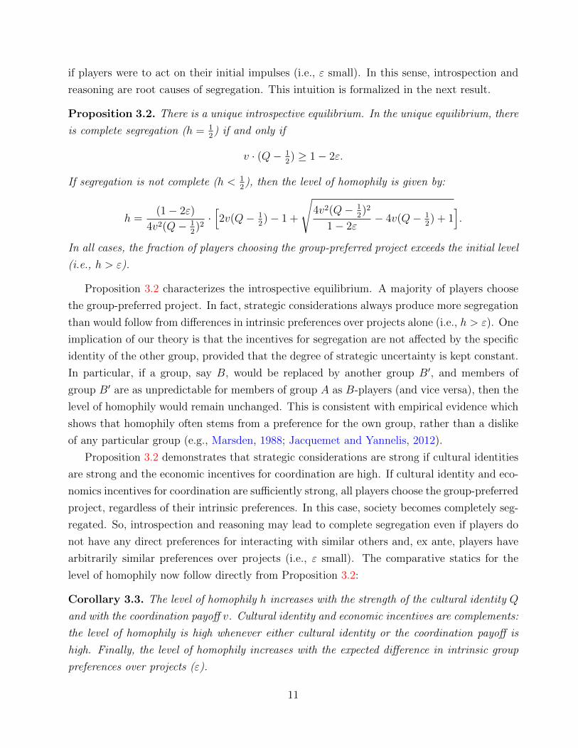
Proposition 3.2. There is a unique introspective equilibrium. In the unique equilibrium, there
is complete segregation (h = 12) if and only if
v · (Q− 12) ≥ 1− 2ε.
If segregation is not complete (h < 12), then the level of homophily is given by:
h =(1− 2ε)
4v2(Q− 12)2·[2v(Q− 1
2)− 1 +
√4v2(Q− 1
2)2
1− 2ε− 4v(Q− 1
2) + 1
].
In all cases, the fraction of players choosing the group-preferred project exceeds the initial level
(i.e., h > ε).
Proposition 3.2 characterizes the introspective equilibrium. A majority of players choose
the group-preferred project. In fact, strategic considerations always produce more segregation
than would follow from differences in intrinsic preferences over projects alone (i.e., h > ε). One
implication of our theory is that the incentives for segregation are not affected by the specific
identity of the other group, provided that the degree of strategic uncertainty is kept constant.
In particular, if a group, say B, would be replaced by another group B′, and members of
group B′ are as unpredictable for members of group A as B-players (and vice versa), then the
level of homophily would remain unchanged. This is consistent with empirical evidence which
shows that homophily often stems from a preference for the own group, rather than a dislike
of any particular group (e.g., Marsden, 1988; Jacquemet and Yannelis, 2012).
Proposition 3.2 demonstrates that strategic considerations are strong if cultural identities
are strong and the economic incentives for coordination are high. If cultural identity and eco-
nomics incentives for coordination are sufficiently strong, all players choose the group-preferred
project, regardless of their intrinsic preferences. In this case, society becomes completely seg-
regated. So, introspection and reasoning may lead to complete segregation even if players do
not have any direct preferences for interacting with similar others and, ex ante, players have
arbitrarily similar preferences over projects (i.e., ε small). The comparative statics for the
level of homophily now follow directly from Proposition 3.2:
Corollary 3.3. The level of homophily h increases with the strength of the cultural identity Q
and with the coordination payoff v. Cultural identity and economic incentives are complements:
the level of homophily is high whenever either cultural identity or the coordination payoff is
high. Finally, the level of homophily increases with the expected difference in intrinsic group
preferences over projects (ε).
11

0.5
0.6
0.7
0.8
0.9
1
0
1
2
3
40
0.1
0.2
0.3
0.4
0.5
Qv
h
Figure 1: The level of homophily h as a function of the coordination payoff v and the strength
of players’ cultural identity Q.
Figure 1 plots the level of homophily as a function of the coordination payoff and the
strength of players’ cultural identity. The level of homophily is determined by both cultural
and economic factors: it increases with economic incentives to coordinate and with cultural
identity. These comparative statics results deliver clear and testable predictions for the model.
One of the key results in this analysis of introspection and reasoning is that similar agents
will tend to successfully coordinate on the project that the majority of their group prefers.
This is intuitive. The project preferred by the majority may be the natural focal point for the
group. However, standard equilibrium analysis delivers a multiplicity of equilibria. Some of
these equilibria are highly inefficient. For example, there is an equilibrium where all players
choose the non-group preferred project (e.g., all A-players choose project b); see Appendix D.
In such equilibria, the majority of players choose a project that they do not intrinsically prefer.
Intuitively, choosing a project constitutes a coordination problem, and inefficient lock-in can
occur in equilibrium. In contrast, when players are introspective, the majority always chooses
the group-preferred project, society avoids inefficient lock-in, and successful coordination on
the payoff-maximizing outcome ensues. In particular, when players are introspective, there is
only one equilibrium. This uniqueness makes it possible to obtain global comparative statics
results.
Diversity-oriented policies involve difficult trade-offs that can be elucidated by this model.
12

Consider the question of whether students dorms should be determined at random or whether
students should be free to select their roommates. In the latter case, students’ expected pay-
offs will be higher, but these higher payoffs will be achieved through segregation. Thus, in
the future, students will continue to have incentives to segregate as they acquire a greater
understanding of those in their groups than of outgroup members. If students are matched
at random, they will experience lower expected payoffs (at least in the short run) but may
gain a greater understanding of people outside their group, reducing strategic uncertainty
in intergroup interactions. This may produce a more inclusive culture that will reduce fu-
ture incentives for segregation. Indeed, the contact hypothesis in sociology states that under
appropriate conditions interpersonal contact is an effective way to reduce prejudice and to
appreciate others’ point of view (Allport, 1954). While the contact hypothesis focuses on prej-
udice, stereotypes, and stigma, it is conceivable that interpersonal contact may also reduce
strategic uncertainty. Thus, in the long run, individuals may be better off in a more integrated
society, even if (partial) segregation is optimal in the long run.
Another rationale for diversity-oriented policies emerges when economic incentives may
change over time. Suppose there is a strong cultural identity, so that the society is fully
segregated (h = 12). Individuals successfully coordinate, and earn high payoffs. Now suppose
the payoffs change, so that coordinating on action s1 gives both players a payoff of 2v, while
coordinating on s2 gives both players a payoff of v. So, option s1 is now payoff dominant. As
before, there is a unique introspective equilibrium. In this unique equilibrium, players follow
their impulse whenever cultural identity is sufficiently strong. So, individuals do not manage
to coordinate exclusively on the payoff dominant outcome. Intuitively, the coordination motive
dwarves any other incentive. Now suppose that society is desegregated, that is, h = 0. Also
in this case, there is a unique introspective equilibrium. However, in this unique equilibrium,
players always coordinate on the payoff dominant option s1, regardless of their initial impulse.
The intuition is that when segregation is limited or even absent, the coordination motive is
weak, so that economic incentives have free rein. In other words, while high levels of homophily
are beneficial in the short run, when the game is fixed, it can lead to excessive conformism
when the game changes.12 This may partly explain why companies often invest considerable
effort into socio-cultural integration after mergers, for example, by transferring key personnel
between units (Shrivastava, 1986).
The goals of developing a more inclusive culture or a more adaptable culture must be
differentiated from another common rationale for diversity-oriented policies: the benefits from
12This result does not depend on the exact payoffs: for any payoff V ∗ > v level for the payoff dominant
option, individuals in a highly segregated society will continue to follow their impulse provided that cultural
identity is sufficiently strong.
13

complementary skills. If players in different groups have complementary skills then the levels
of segregation are reduced even in absence of any diversity-oriented policy. This can easily be
shown with our basic methodology. To incorporate complementary skills, assume that players
receive a payoff v > 0 if they coordinate with a member of their own group, and a payoff
V ≥ v if they coordinate with a member of the other group (and 0 otherwise). We analyze
this setting using the exact same approach as before. The next result shows that introspection
and reasoning lead to homophily when cultural identities and coordination payoffs are strong
relative to the rewards to skill complementarity.
Proposition 3.4. There is a unique introspective equilibrium, characterized by the limiting
probability p whenever Qv − 12V > −1
2.13 The level of homophily h decreases with V and
exceeds the initial level (i.e., h > ε) if and only if Qv > 12V .
Proposition 3.4 shows that as skill complementarity grows, the level of homophily falls, and
groups tend to be more integrated. On the other hand, as shown before, homophily increases
as the payoffs for coordination increase. In many organizations, productivity may depend on
both coordination and skill complementarity (Milliken and Martins, 1996). Thus, rewarding
teams based on their productivity alone, may increase or decrease homophily depending on
whether productivity relies more on coordination or on skill complementarity.
Finally, so far we have assumed that players can recognize the group of their opponents. If
group type is not observable then players can use markers, that is, observable attributes such
as tattoos or specific attire, to signal their identity. This helps explain why groups are often
marked by seemingly arbitrary traits (Barth, 1969). The model in which players first choose
markers, say a and b, and then play the coordination game is very similar to the model in
this section (with markers replacing projects) and is available from the authors upon request.
The comparative statics results are analogous and, once again, strong cultural identity and
economic incentives for coordination are driving forces for homophily. If cultural identity and
coordination payoffs are sufficiently strong, then complete segregation arises even if group
identity is unobservable, there are no direct preferences for interacting with members of the
same group and there is only a small tendency for A-players to intrinsically prefer marker a
and B-players to prefer marker b.
13If Qv− 12V −
12 , the sequence pπ0 , p
π1 , . . . does not settle down. Intuitively, the game bears some similarities
with a congestion game, with players fleeing from players of their own group to reap the high payoffs from
interacting with the other group. This leads to a large share of players switching continually between projects.
14

4. Network formation
In many situations, people can choose how many people they interact with. We extend the
basic model to allow players to choose how much effort they want to invest in meeting others.
We show that the basic mechanisms that drive the tendencies to segregate may be reinforced,
and that the model gives rise to network properties that are commonly observed in social and
economic networks.
To analyze this setting, it will be convenient to work with a finite (but large) player set in
this section.14 Each group G = A,B has N players, so that the total number of players is 2N .
Players simultaneously choose effort levels and projects in the first stage. They then interact
in the coordination game. Effort is costly: a player that invests effort e pays a cost ce2/2. By
investing effort, however, a player meets more partners to play the coordination game with
(in expectation). Specifically, if two players j, ` have chosen the same project π = a, b, and
invest effort ej and e`, respectively, then the probability that they are matched (and play the
coordination game) isej · e`Eπ
,
where Eπ is the total effort of the players with project π.15 Thus, efforts are complements:
players meet each other only if they both invest the time and the resources. This is related
to the assumption of bilateral consent in deterministic models of network formation (Jackson
and Wolinsky, 1996). By normalizing by the total effort Eπ, we ensure that the network does
not become arbitrarily dense as the number of players grows large.16 So, the probability p of
being matched with a member of the own group is endogenous here, as in Section 3. Matching
probabilities are now affected not only by players’ project choice, as in Section 3, but also by
their effort levels.
As before, at level 0 players choose the project that they intrinsically prefer. So, the
probability that a player chooses the group-preferred project is 12
+ ε. In addition, each player
chooses some default effort e0 > 0, independent of his project or group. At higher levels k,
each player formulates a best response to the choices at level k − 1. As before, each player
receives a (single) signal that tells him which action is appropriate in the coordination game.
14Defining networks with a continuum of players gives rise to technical problems. Our results in Sections
2 and 3 continue to hold under the present formulation of the model (with a finite player set), though the
notation becomes more tedious.15To be precise, to get a well-defined probability, if Eπ = 0, we take the probability to be 0; and if ej ·e` > Eπ,
we take the probability to be 1.16See, e.g., Cabrales et al. (2011) and Galeotti and Merlino (2014) for other applications of this model in
economics.
15

He then plays the coordination game with each of the players he is matched to.17
A first result is that the limiting behavior is well-defined, and that it is independent of the
choice of effort at level 0.
Lemma 4.1. The limiting probability p and the limiting effort choices exist and do not depend
on the effort choice at level 0.
As before, we have a unique introspective equilibrium, with potentially high levels of
homophily:
Proposition 4.2. There is a unique introspective equilibrium. In the unique equilibrium,
all players choose positive effort. Players that have chosen the group-preferred project exert
strictly more effort than players with the other project. In all cases, the fraction of players
choosing the group-preferred project exceeds the initial level (i.e., h > ε).
As before, players segregate for strategic reasons and the level of homophily is greater than
what would be expected on the basis of intrinsic preferences alone (i.e., h > ε). Importantly,
players with the group-preferred project invest more effort in equilibrium than players with the
other project. This is intuitive: a player with the group-preferred project has a high chance
of meeting people from her own group, and thus a high chance of coordinating successfully.
In turn, this reinforces the incentives to segregate.
Figure 2 illustrates the comparative statics of the unique equilibrium. As before, the
level of homophily increases with the strength of players’ cultural identity and with economic
incentives, and the two are complements. While the proof of Proposition 4.2 provides a full
characterization of the equilibrium, the comparative statics cannot be analyzed analytically,
as the effort levels and the level of homophily depend on each other in intricate ways. In the
remainder of this section, we therefore focus on deriving analytical results for the case where
the network becomes arbitrarily large (i.e., |N | → ∞). As a first step, we give an explicit
characterization of the unique introspective equilibrium:
Proposition 4.3. Consider the limit where the number of players in each group goes to infin-
ity. The effort chosen by the players with the group-preferred project in the unique introspective
equilibrium converges to
e∗ =v
4c·
(1 + 2Q− 1
2h+
√4Q2 − 1 +
1
4h2
),
17We allow players to take different actions in each of the (two-player) coordination games he is involved in.
Nevertheless, in any introspective equilibrium, a player chooses the same action in all his interactions, as it is
optimal for him to follow his impulse (Proposition 2.1).
16

0
1
2
3
4
5
0.50.55
0.60.65
0.70.75
0.80.85
0.90.95
1
0
0.05
0.1
0.15
0.2
0.25
0.3
0.35
0.4
0.45
0.5
vQ
h
Figure 2: The level of homophily h as a function of the coordination payoff v and the strength
of players’ cultural identity Q (c = 1).
while the effort chosen by the players with the other project converges to
e− =v
c· (Q+ 1
2)− e∗,
which is strictly smaller than the effort e∗ (while positive).
Proposition 4.3 shows that in the unique introspective equilibrium, the effort levels depend
on the level of homophily. The level of homophily, in turn, is a function of the equilibrium
effort levels. For example, by increasing her effort, an A-player with the group-preferred
project a increases the probability that players from both groups interact with her and thus
with members from group A. This makes project a more attractive for members from group
A, strengthening the incentives for players from group A to choose project a, and this leads
to higher levels of homophily. Conversely, if more players choose the group-preferred project,
this strengthens the incentives of players with the group-preferred project to invest effort, as
it increases their chances of meeting a player from their own group. This, in turn, further
increases the chances for players with the group-preferred project of meeting someone from
the own group, reinforcing the incentives to segregate. On the other hand, if effort is low, then
17

then the incentives to segregate are attenuated, as the probability of meeting similar others is
small. This, in turn, reduces the incentives to invest effort.
As a result of this feedback loop, there are two different regimes. If effort costs are small
relative to the benefits of coordinating, then players are willing to exert high effort, which in
turn leads more players to choose the group-preferred project, further enhancing the incentives
to invest effort. In that case, groups are segregated, and players are densely connected.
Importantly, players with the group-preferred project face much stronger incentives to invest
effort than players with the other project, as players with the group-preferred project have
a high chance of interacting with players from their own group. On the other hand, if effort
costs are sufficiently high, then the net benefit of interacting with others is small, even if
society is fully segregated. In that case, choices are guided primarily by intrinsic preferences
over projects, and the level of homophily is low. As a result, players face roughly the same
incentives to invest effort, regardless of their project choice, and all players have approximately
the same number of connections. Hence, high levels of homophily go hand in hand with
inequality in the number of connections that players have. The following result makes this
precise:
Proposition 4.4. Consider the limit where the number of players in each group goes to in-
finity. In the unique introspective equilibrium, the distribution of connections of players with
the group-preferred project first-order stochastically dominates the distribution of the number
of connections of players with the other project. Moreover, the expected number of connections
of a player with the group-preferred project is e∗, and the expected number of connections of
the other players is e− < e∗. The gap e∗− e− in the expected number of connections is greater
if the equilibrium level of homophily is greater.
The result follows directly from Proposition 4.2 and Theorem 3.13 of Bollobas et al. (2007).
These results are consistent with empirical evidence. It has been widely documented that the
distribution of the number of connections in social and economic networks has considerable
variance (Jackson, 2008). Furthermore, consistent with the theoretical results, friendships
are often biased towards own-group friendships, and larger groups form more friendships per
capita (Currarini et al., 2009).
Our results thus put restrictions on the type of networks that can be observed. When
relative benefits v/c are high and there is a strong cultural identity Q, then networks are dense
and are characterized by high levels of homophily and a skewed distribution of the number
of connections that players have. Moreover, the network consists of a tightly connected core
of players from one group, with a small periphery of players from the other group. When
v/c increases further, segregation is complete (h = 12), and a densely connected homogenous
18

network results. On the other hand, when economic benefits are limited and cultural identity
is weak, networks are disconnected, and feature low levels of homophily and limited variation
in the number of connections. Most data on network on social and economic networks is
consistent with the case where there is a strong cultural identity and sizeable economic benefits
to coordination, with many networks featuring high levels of homophily, a core-periphery
structure, high levels of connectedness, and a skewed degree distribution (Jackson, 2008).
More research is needed, of course, to establish to what extent these observations can indeed
be attributed to the economic and cultural factors that drive players’ preferences for reducing
strategic uncertainty.
5. Conclusions
We introduced a novel approach to model players’ introspective process, grounded in ev-
idence from psychology, that allows unique predictions in settings where individuals form
connections and want to reduce strategic uncertainty. We show that high levels of segregation
are possible even in the absence of any preferences for interactions with similar others. Con-
sistently with empirical and experimental evidence, homophily is high when cultural identities
are strong and when there are substantial benefits from coordination. Homophily can be even
higher if networks are formed endogenously. The theory also elucidates the tradeoffs inherent
in diversity-oriented policies. In particular, if skill complementarity or flexibility is important,
welfare is higher when the society is more integrated. Also, overall strategic uncertainty may
be reduced if a society becomes more integrated.
The results in this paper open up new perspectives. One question is whether strategic
uncertainty leads players to associate with similar others, and how this motive compares to
other potential drivers of homophily, such as social preferences. This question is addressed
in a companion experimental paper, Kets et al. (2014). Another question is how to develop
a general methodology, based on introspection and the Theory of Mind, capable of making
sharp predictions and global comparative statics results in general strategic situations. We
leave this question for future research.
Appendix A Introspection: The case of beliefs
Experimental evidence suggests that people intuitively think about other minds in terms
of the capacity to act or the capacity to have beliefs and emotions (Gray et al., 2007). In the
main text, we developed a model that takes beliefs about another player’s action as a starting
19

point; here, we sketch a model that starts with players’ beliefs about others’ beliefs. So, while
in the main text, we focus on the case where players have an impulse to act (and subsequently
realize that others may have a similar impulse), here, the order is reversed: a player empathizes
with the other player and thinks about how his opponent thinks first, before forming a belief
about his opponent’s action and formulating a best response. This alternative model gives
the same result: when players are introspective and focal points are context-dependent, it is
optimal for players to follow their impulse, where following one’s impulse now means playing
a best response to one’s initial belief.
As before, we focus on a symmetric pure coordination game. It will be convenient to
denote the action set by S := {s1, s2}. For simplicity, we use the same setting as before: each
group is characterized by a state, and player’s impulses are informative about the state (and
thus about the other players’ impulses). There are two states, λ and ν, and states are drawn
independently across groups according to the uniform distribution. Impulses take the form of
beliefs about the opponent’s beliefs. For simplicity, we assume that a player can have one of
two possible initial beliefs about her partner: either she thinks it is likely that he thinks it is
likely that she chooses s1, or she thinks it is likely that he thinks it is likely that she plays s2.
So, let λ0 be probability measure that assigns probability x > 12
to the event that the other
player assigns probability at least y to the event that his partner chooses s1 (and 1− x to the
complementary event); likewise, ν0 is the probability measure that assigns probability x > 12
to the event that the other player assigns probability y > 12
to the event that his partner
chooses s2. Conditional on the group’s state being θG = λ, a player has initial belief λ0 with
probability q > 12, independent across players; the analogous statement applies when θG = ν.
For a player to take a rational decision, she has to form a belief about her opponent’s
action, that is, a first-order belief. If she thinks her opponent is rational, then she must think
he chooses s whenever that action is a best response to his belief. So, if a player has initial
belief z0 = λ0, ν0 and believes that her opponent is rational, then the beliefs she can have
about his action are given by
M1(z0) := {µ ∈ ∆(S) : for all s ∈ S, µ(s) ≥ z0({µ1 ∈ ∆(S) : s is a strict best response to µ1})},
where ∆(X) is the set of Borel probabilities on a set X.18 Define
M1 := M1(λ0) ∪M1(ν0)
to be the set of all such first-order beliefs. At higher orders, players believe that an opponent
from the same group has the same initial belief with probability Q = q2 + (1− q)2, and that
18The set S is endowed with its usual discrete topology, and for any topological space X, the set ∆(X) of
Borel probability measures on X is endowed with the weak convergence topology. Also, we endow subspaces
and product spaces of topological spaces with their usual relative an product topologies, respectively.
20
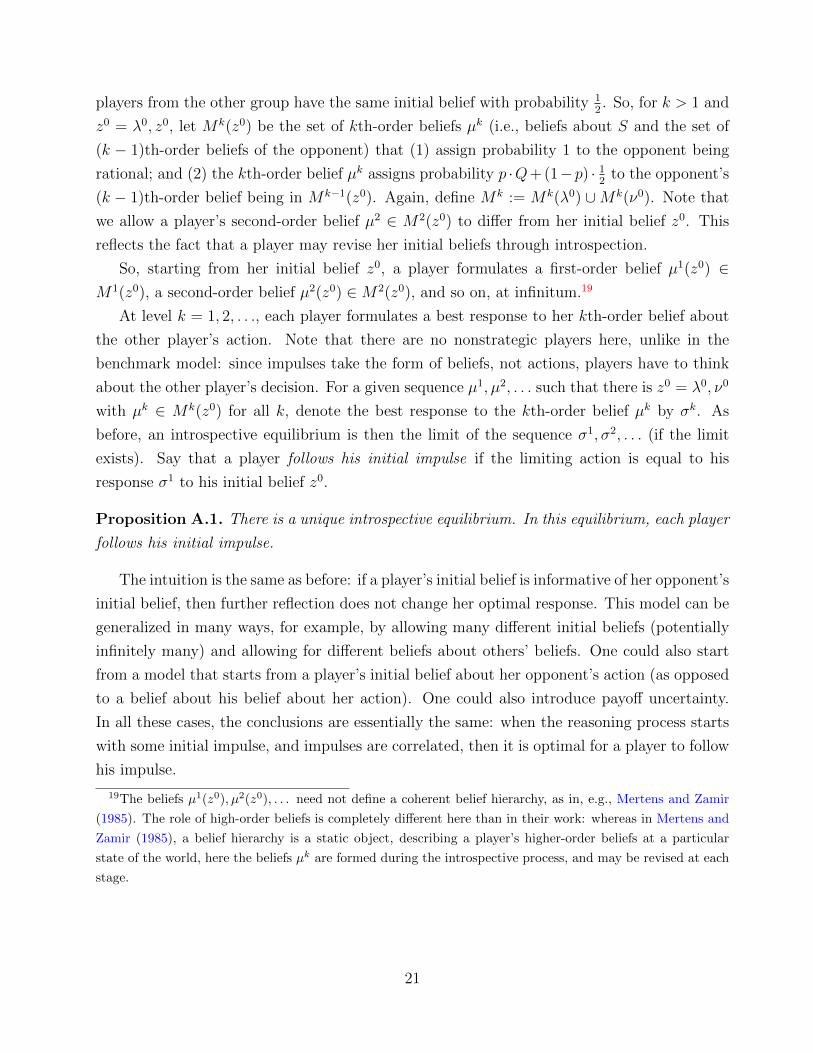
players from the other group have the same initial belief with probability 12. So, for k > 1 and
z0 = λ0, z0, let Mk(z0) be the set of kth-order beliefs µk (i.e., beliefs about S and the set of
(k − 1)th-order beliefs of the opponent) that (1) assign probability 1 to the opponent being
rational; and (2) the kth-order belief µk assigns probability p ·Q+ (1−p) · 12
to the opponent’s
(k − 1)th-order belief being in Mk−1(z0). Again, define Mk := Mk(λ0) ∪Mk(ν0). Note that
we allow a player’s second-order belief µ2 ∈ M2(z0) to differ from her initial belief z0. This
reflects the fact that a player may revise her initial beliefs through introspection.
So, starting from her initial belief z0, a player formulates a first-order belief µ1(z0) ∈M1(z0), a second-order belief µ2(z0) ∈M2(z0), and so on, at infinitum.19
At level k = 1, 2, . . ., each player formulates a best response to her kth-order belief about
the other player’s action. Note that there are no nonstrategic players here, unlike in the
benchmark model: since impulses take the form of beliefs, not actions, players have to think
about the other player’s decision. For a given sequence µ1, µ2, . . . such that there is z0 = λ0, ν0
with µk ∈ Mk(z0) for all k, denote the best response to the kth-order belief µk by σk. As
before, an introspective equilibrium is then the limit of the sequence σ1, σ2, . . . (if the limit
exists). Say that a player follows his initial impulse if the limiting action is equal to his
response σ1 to his initial belief z0.
Proposition A.1. There is a unique introspective equilibrium. In this equilibrium, each player
follows his initial impulse.
The intuition is the same as before: if a player’s initial belief is informative of her opponent’s
initial belief, then further reflection does not change her optimal response. This model can be
generalized in many ways, for example, by allowing many different initial beliefs (potentially
infinitely many) and allowing for different beliefs about others’ beliefs. One could also start
from a model that starts from a player’s initial belief about her opponent’s action (as opposed
to a belief about his belief about her action). One could also introduce payoff uncertainty.
In all these cases, the conclusions are essentially the same: when the reasoning process starts
with some initial impulse, and impulses are correlated, then it is optimal for a player to follow
his impulse.
19The beliefs µ1(z0), µ2(z0), . . . need not define a coherent belief hierarchy, as in, e.g., Mertens and Zamir
(1985). The role of high-order beliefs is completely different here than in their work: whereas in Mertens and
Zamir (1985), a belief hierarchy is a static object, describing a player’s higher-order beliefs at a particular
state of the world, here the beliefs µk are formed during the introspective process, and may be revised at each
stage.
21

Appendix B Distribution of intrinsic preferences
We denote the values of an A-player j for projects a and b are denoted by wA,aj and
wA,bj , respectively; likewise, the values of a B-player for projects b and a are wB,bj and wB,aj ,
respectively. As noted in the main text, the values wA,aj and wA,bj are drawn from the uniform
distribution on [0, 1] and [0, 1 − 2ε], respectively. Likewise, wB,bj and wB,aj are uniformly
distributed on [0, 1] and [0, x]. All values are drawn independently (across players, projects,
and groups). So, players in group A (on average) intrinsically prefer project a (in the sense of
first-order stochastic dominance) over project b; see Figure 3. Likewise, on average, players in
group B have an intrinsic preference for b.
−0.2 0 0.2 0.4 0.6 0.8 1 1.20
0.1
0.2
0.3
0.4
0.5
0.6
0.7
0.8
0.9
1
y
Pro
b(w
jA,a
≤ y)
, Pro
b(w
jA,b
≤ y)
Figure 3: The cumulative distribution functions of wA,ai (solid line) and wA,bi (dashed line) for
x = 0.75.
Given that the values are uniformly and independently distributed, the distribution of the
difference wA,aj −wB,aj in values for an A-player is given by the so-called trapezoidal distribution.
That is, if we define x := 1−2ε, we can define the tail distribution Hε(y) := P(wA,aj −wA,bj ≥ y)
by
Hε(y) =
1 if y < −(1− 2ε);
1− 12−4ε · (1− 2ε+ y)2 if y ∈ [−(1− 2ε), 0);
1− 12· (1− 2ε)− y if y ∈ [0, 2ε);
1
4(12−ε)· (1− y)2 if y ∈ [2ε, 1];
0 otherwise.
By symmetry, the probability P(wB,bj −wB,aj ≥ y) that the difference in values for the B-player
22

is at least y is also given by Hε(y). So, we can identify wA,aj − wA,bj and wB,bj − wB,aj with the
same random variable, denoted ∆j, with tail distribution Hε(·); see Figure 4.
00
y
Pro
b(w
A,a
j −
wA
,bj
≥ y
)
Figure 4: The probability that wA,aj − wA,bj is at least y, as a function of y, for ε = 0 (solid
line); ε = 0.125 (dotted line); and ε = 0.375 (dashed line).
The probability that A-players prefer the a-project, or, equivalently, the share of A-players
that intrinsically prefer a (i.e., wA,aj −wA,bj > 0), is 1− 1
2x, and similarly for the B-players and
their group-preferred project.
Appendix C Proofs
C.1 Proof of Proposition 2.1
By assumption, at level 0, a player chooses action si if and only if his initial impulse is
i = 1, 2. For k > 0, assume, inductively, that at level k − 1, a player chooses si if and only
if his initial impulse is i. Consider level k, and suppose a player’s impulse is i. Choosing si
is the unique best response for him if the expected payoff from choosing si is strictly greater
than the expected payoff from choosing the other action sj 6= si. That is, if we write j 6= i for
the alternate impulse, si is the unique best response for the player if[p · P(i | i) + (1− p) · P(i)
]· v >
[p · P(j | i) + (1− p) · P(j)
]· v,
where P(m | i) is the conditional probability that the impulse of a player from the same group
is m = 1, 2 given that the player’s own impulse is i, and P(m) is the probability that a player
from the other group has received signal m. Using that P(m) = 12, P(i | i) = q2 + (1− q)2 and
P(j | i) = 1− q2 − (1− q)2, and rearranging, we find that this holds if and only if
p(q2 + (1− q)2) + 12(1− p) > p(1− q2 − (1− q)2) + 1
2(1− p),
23

and this holds for every p > 0, since q2 + (1− q)2 > 12.
This shows that at each level, it is optimal for a player to follow his impulse. So, in the
unique introspective equilibrium, every player follows his impulse. �
C.2 Proof of Lemma 3.1
We show that the sequence {pπk}k is (weakly) increasing and bounded for every project
π. It will be useful to define β := v · (Q − 12). It can be checked that β is the derivative of
the expected payoff of a player in the introspective equilibrium with respect to p. So, β is
the marginal benefit of interacting with the own group. Also, recall from Appendix B that
x := 1− 2ε.
First note that for every k > 0, given pak−1, a player from group A chooses project A if and
only if [pak−1 ·Q+ (1− pak−1) · 12
]· v + wA,aj ≥
[(1− pak−1) ·Q+ pak−1 · 12
]· v + wA,bj .
This inequality can be rewritten as
wA,aj − wA,bj ≥ −(2pak−1 − 1) · β,
and the share of A-players for whom this holds is
pak := Hε
(−(2pk−1 − 1) · β
),
where we have used the expression for the tail distribution Hε from Appendix B. The same
law of motion holds, of course, if a is replaced with b and A is replaced with B.
Fix a project π. Notice that −(2pπ0−1) ·β < 0. We claim that pπ1 ≥ pπ0 and that pπ1 ∈ (12, 1].
By the argument above,
pπ1 = P(wA,aj − wA,bj ≥ −(2pπ0 − 1) · β)
= Hε(−(2pπ0 − 1) · β)
=
{1− 1
2−4ε · (1− 2ε− (2pπ0 − 1) · β)2 if (2pπ0 − 1) · β ≤ 1− 2ε;
1 if (2pπ0 − 1) · β > 1− 2ε;
where we have used the expression for the tail distribution Hε(y) from Appendix B. If (2pπ0 −1) · β > 1 − 2ε, the result is immediate, so suppose that (2pπ0 − 1) · β ≤ 1 − 2ε. We need to
show that
1− 12−4ε · (1− 2ε− (2pπ0 − 1) · β)2 ≥ pπ0 .
Rearranging and using that pπ0 ∈ (12, 1], we see that this holds if and only if
(2pπ0 − 1) · β ≤ 2 · (1− 2ε).
24

But this holds because (2pπ0 − 1) ·β ≤ 1− 2ε and 1− 2ε ≥ 0. Note that the inequality is strict
whenever β < 1− 2ε, so that pπ1 > pπ0 in that case.
For k > 1, suppose, inductively, that pπk−1 ≥ pπk−2 and that pπk−1 ∈ (12, 1]. By a similar
argument as above,
pπk =
{1− 1
2−4ε · (1− 2ε− (2pπk−1 − 1) · β)2 if (2pπk−1 − 1) · β ≤ 1− 2ε;
1 if (2pπk−1 − 1) · β > 1− 2ε.
Again, if (2pπk−1− 1) · β > 1− 2ε, the result is immediate, so suppose (2pπk−1− 1) · β ≤ 1− 2ε.
We need to show that
1− 12−4ε · (1− 2ε− (2pπk−1 − 1) · β)2 ≥ pπk−1,
or, equivalently,
2 · (1− 2ε) · (1− pπk−1) ≥ (1− 2ε− (2pπk−1 − 1) · β)2.
By the induction hypothesis, pπk−1 ≥ pπ0 , so that 1− 2ε ≥ 2− 2pπk−1. Using this, we have that
2 · (1− 2ε) · (1− pπk−1) ≥ 4 · (1− pπk−1)2. Moreover,
(1− 2ε− (2pπk−1 − 1) · β)2 ≤ 4 · (1− pπk−1)2 − 2β(1− 2ε)(2pπk−1 − 1) + (2pπk−1 − 1)2β2.
So, it suffices to show that
4 · (1− pπk−1)2 ≥ 4 · (1− pπk−1)2 − 2β(1− 2ε)(2pπk−1 − 1) + (2pπk−1 − 1)2β2.
The above inequality holds if and only if
(2pπk−1 − 1)β ≤ 2 · (1− 2ε),
and this is true since (2pπk−1 − 1) · β ≤ 1− 2ε.
So, the sequence {pπk}k is weakly increasing and bounded. It now follows from the monotone
sequence convergence theorem that the limit pπ exists. The argument clearly does not depend
on the project π, so we have pa = pb. �
C.3 Proof of Proposition 3.2
We first characterize the limiting fraction p, and show that p > 12
+ ε. By the proof of
Lemma 3.1, we have pk ≥ pk−1 for all k. By the monotone sequence convergence theorem,
p = supk pk, and by the inductive argument, p ∈ (12
+ ε, 1]. It is easy to see that p = 1 if and
only if Hε(−(2 · 1− 1) · β) = 1, which holds if and only if β ≥ 1− 2ε.
25

So suppose that β < 1 − 2ε, so that p < 1. Again, p = Hε(−(2p − 1) · β), or, using the
expression from Appendix B,
p = 1− 12−4ε · (1− 2ε− (2p− 1) · β)2.
It will be convenient to substitute x = 1− 2ε for ε, so that we are looking for the solution of
p = 1− 12x· (x− (2p− 1) · β)2. (C.1)
Equation (C.1) has two roots,
r1 = 12
+ 14β2
((2β − 1) · x+
√4β2x− (4β − 1) · x2
)and
r2 = 12
+ 14β2
((2β − 1) · x−
√4β2x− (4β − 1) · x2
).
We first show that r1 and r2 are real numbers, that is, that 4β2x − (4β − 1) · x2 ≥ 0. Since
x > 0, this is the case if and only if 4β ≥ (4β − 1) · x. This holds if β ≤ 14, so suppose that
β > 14. We need to show that
x ≤ 4β2
4β − 1.
Since the right-hand side achieves its minimum at β = 12, it suffices to show that x ≤ (4 ·
(12)2)/(4 · 1
2− 1) = 1. But this holds by definition. It follows that r1 and r2 are real numbers.
We next show that r1 >12, and r2 <
12. This implies that p = r1, as p = supk pk > p0 >
12.
It suffices to show that 4β2x − (4β − 1) · x2 > (1 − 2β)2x2. This holds if and only if
β > (2 − β) · x. Recalling that β ≤ 1 − 2ε < 1 by assumption, we see that this inequality is
satisfied. We conclude that p = r1. �
As for the comparative statics in Corollary 3.3, it is straightforward to verify that the
derivative of p with respect to v · (Q − 12)) is positive whenever p < 1 (and 0 otherwise). It
then follows from the chain rule that the derivatives of p with respect to v and Q are both
positive for any p < 1 (and 0 otherwise).
C.4 Proof of Lemma 4.1
Recall that at level 0, players invest effort e0 > 0 in socializing. Moreover, they choose
project a if and only if they intrinsically prefer project a over project b. It follows from the
distribution of the intrinsic values (Appendix B) that the number NA,a0 of A-players with
project a at level 0 follows the same distribution as the number NB,b0 of B-players with project
b at level 0; similarly, the number NA,a0 of A-players with project b at level 0 has the same
distribution as the number NB,a0 of B-players with project a at level 0. Let ND
0 and NM0 be
26

random variables with the same distribution as NA,a0 and NB,a
0 , respectively (where D stands
for “dominant group” and M stands for “minority group”; the motivation for this terminology
is that a slight majority of the players with an intrinsic preference for project a belongs to
group A).
Conditional on ND0 and NM
0 , the expected utility of project a to an A-player at level 1 is20
v ·[ej ·ND
0 · e0 ·Q+ ej ·NM0 · e0 · 12
ND0 · e0 +NM
0 · e0
]+ wA,aj − cej
2
if he invests effort ej and his intrinsic value for project a is wA,aj . Likewise, conditional on ND0
and NM0 , the expected utility of project b to an A-player at level 1 is
v ·[ej ·NM
0 · e0 ·Q+ ej ·ND0 · e0 · 12
ND0 · e0 +NM
0 · e0
]+ wA,bj −
cej2
if he invests effort ej and his intrinsic value for project b is wA,bj . Taking expectations over
ND0 and NM
0 , it follows from the first-order conditions that the optimal effort levels for an
A-player at level 1 with projects a and b are given by
eA,a1 =(vc
)· E[ND
0 · e0 ·Q+NM0 · e0 · 12
ND0 · e0 +NM
0 · e0
]; and
eA,b1 =(vc
)· E[NM
0 · e0 ·Q+ND0 · e0 · 12
ND0 · e0 +NM
0 · e0
];
respectively, independent of the intrinsic values. It can be checked that the optimal effort
levels eB,a1 and eB,b1 for a B-player at level 1 with projects a and b are equal to eA,b1 and eA,a1 ,
respectively. It will be convenient to define eD1 := eA,a1 = eB,b1 and eM1 := eA,b1 = eB,a1 . We claim
that eD1 > eM1 . To see this, note that ND0 is binomially distributed with parameters |N | and
p0 := 12+ε > 1
2(the probability that a player has an intrinsic preference for the group-preferred
project) and that NM0 is binomially distributed with parameters |N | and 1 − p0 < 1
2. If we
define
gD1 (ND0 , N
M0 , e0) :=
(vc
)·(ND
0 · e0 ·Q+NM0 · e0 · 12
ND0 · e0 +NM
0 · e0
); and
gM1 (ND0 , N
M0 , e0) :=
(vc
)·(NM
0 · e0 ·Q+ND0 · e0 · 12
ND0 · e0 +NM
0 · e0
);
so that eD1 and eM1 are just the expectations of gD1 and gD1 , respectively, then the result follows
immediately from the fact that ND0 first-order stochastically dominates NM
0 , as gD1 is (strictly)
20If ND0 = NM
0 = 0, then the expected benefit from networking is 0. In that case, the player’s expected
utility is thus wA,aj − cej2 . A similar statement applies at higher levels.
27

increasing in ND0 and (strictly) decreasing in NM
0 , and gM1 is decreasing in ND0 and increasing
in NM0 (again, strictly).
Substituting the optimal effort levels eD1 and eM1 into the expression for the expected utility
for each project shows that the maximal expected utility of an A-player at level 1 of projects
a and b is given by
c
2(eD1 )2 + wA,aj ; and
c
2(eM1 )2 + wA,bj ;
respectively. At level 1, an A-player therefore chooses project a if and only if
wA,aj − wA,bj ≥ − c2
((eD1 )2 − (eM1 )2
).
The analogous argument shows that a B-player chooses project b at level 1 if and only if
wB,bj − wB,aj ≥ − c
2
((eD1 )2 − (eM1 )2
).
Since wA,aj −wA,bj and wB,bj −w
B,aj both have tail distribution Hε(·) (Appendix B), the proba-
bility that an A-player chooses project a (or, that a B-player chooses project b) is
p1 := Hε
(− c
2
((eD1 )2 − (eM1 )2
)).
Since eD1 > eM1 , we have p1 > p0. Note that both the number NA,a1 of A-players at level 1
with project a and the number NB,b1 of B-players at level 1 with project b are binomially
distributed with parameters |N | and p1 >12; the number NA,a
1 of A-players at level 1 with
project b and the number NB,a1 of B-players at level 1 with project a are both binomially
distributed with parameters |N | and 1 − p1. Let ND1 and NM
1 be random variables that are
binomially distributed with parameters (|N |, p1) and (|N |, 1 − p1), respectively, so that the
distribution of ND1 first-order stochastically dominates the distribution of NM
1 .
Note that while NA,a1 and NA,a
1 are clearly not independent (as NA,a1 + NA,a
1 = N), NA,a1
and NB,a1 are independent (and similarly if we replace NA,a
1 , NA,a1 , and NB,a
1 with NB,b1 , NB,a
1 ,
and NA,a1 , respectively). When we take expectations over the number of players from different
groups with a given project (e.g., NA,a1 and NB,a
1 ) to calculate optimal effort levels, we therefore
do not have to worry about correlations between the random variables. A similar comment
applies to levels k > 1.
Finally, it will be useful to note that
eD1 + eM1 =v
c(Q+ 1
2).
28

Both eD1 and eM1 are positive, as they are proportional to the expectation of a nonnegative
random variable (with a positive probability on positive realizations), and we have
eD1 − eM1 > eD0 − eM0 = 0,
where eD0 = eM0 = e0 are the effort choices at level 0.
For k > 1, assume, inductively, that the following hold:
• we have pk−1 ≥ pk−2;
• the number NA,ak−1 of A-players with project a at level k − 1 and the number NB,b
k−1 of
B-players with project b at level k − 1 are binomially distributed with parameters |N |and pk−1;
• the number NA,ak−1 of A-players with project b at level k − 1 and the number NB,a
k−1 of
B-players with project a at level k − 1 are binomially distributed with parameters |N |and 1− pk−1;
• for every level m ≤ k−1, the optimal effort level at level m for all A-players with project
a and for all B-players with project b is equal to eDm;
• for every level m ≤ k−1, the optimal effort level at level m for all A-players with project
b and for all B-players with project a is equal to eMm ;
• we have eDk−1 > eMk−1 > 0 for k ≥ 2;
• we have eDk−1 − eMk−1 ≥ eDk−2 − eMk−2.
We write NDk−1 and NM
k−1 for random variables that are binomially distributed with param-
eters (|N |, pk−1) and (|N |, 1− pk−1), respectively.
By a similar argument as before, it follows that the optimal effort level for an A-player
that chooses project a or for a B-player that chooses b is
eDk :=(vc
)· E[NDk−1 · eDk−1 ·Q+NM
k−1 · eMk−1 · 12NDk−1 · eDk−1 +NM
k−1 · eMk−1
],
and that the optimal effort level for an A player that chooses project b or for a B-player that
chooses a is
eMk :=(vc
)· E[NMk−1 · eMk−1 ·Q+ND
k−1 · eDk−1 · 12NDk−1 · eDk−1 +NM
k−1 · eMk−1
].
Again, it is easy to verify that
eDk + eMk =v
c(Q+ 1
2). (C.2)
29

We claim that eDk ≥ eDk−1 (so that eMk ≤ eMk−1). It then follows from the induction hypothesis
that eDk > eMk and that eDk − eMk ≥ eDk−1 − eMk−1.To show this, recall that form = 1, . . . , k−1, we have that eDm > eMm and eDm+eMm = v
c(Q+ 1
2).
Define
gDk−1(NDk−2, N
Mk−2, e
Dk−2) :=
(vc
)·(NDk−2 · eDk−2 ·Q+NM
k−2 · eMk−2 · 12NDk−2 · eDk−2 +NM
k−2 · eMk−2
)gDk (ND
k−1, NMk−1, e
Dk−1) :=
(vc
)·(NDk−1 · eDk−1 ·Q+NM
k−1 · eMk−1 · 12NDk−1 · eDk−1 +NM
k−1 · eMk−1
)so that eDk−1 and eDk are just proportional to the expectation of gDk−1 and gDk (over ND
k−1 and
NMk−1), respectively, analogous to before. It is easy to verify that gDk (ND
k−1, NMk−1, e
Dk−1) ≥
gDk (NDk−1, N
Mk−1, e
Mk−1). Consequently,
eDk ≥(vc
)· E[NDk−1 · eMk−1 ·Q+NM
k−1 · eMk−1 · 12NDk−1 · eMk−1 +NM
k−1 · eMk−1
]=
(vc
)· E[NDk−1 ·Q+NM
k−1 · 12NDk−1 +NM
k−1
].
Using that gDk is decreasing in its second argument, and that the distribution of NMk−2 first-order
stochastically dominates the distribution of NMk−1, we have
eDk ≥(vc
)· E[NDk−1 ·Q+NM
k−2 · 12NDk−1 +NM
k−2
]. (C.3)
From the other direction, use that gDk−1(NDk−2, N
Mk−2, e
Mk−2) ≤ gDk−1(N
Dk−2, N
Mk−2, e
Dk−1) to obtain
eDk−1 ≤(vc
)· E[NDk−2 · eDk−2 ·Q+NM
k−2 · eDk−2 · 12NDk−2 · eDk−2 +NM
k−2 · eDk−2
].
Using that gDk−1 is increasing in its first argument, and that the distribution of NDk−1 first-order
stochastically dominates the distribution of NDk−2, we obtain
eDk−1 ≤(vc
)· E[NDk−1 ·Q+NM
k−1 · 12NDk−1 +NM
k−1
]. (C.4)
The result now follows by comparing Equations (C.3) and (C.4). Also, using that gDk is
increasing and decreasing in its first and second argument, respectively, we have that
eDk ≥(vc
)· E[N · eMk−1 · 12N · eMk−1
]=
v
2c
eDk ≤(vc
)· E[N · eDk−1 ·QN · eDk−1
]=v ·Qc
,
30

and it follows from (C.2) that eDk , eMk ∈ [ v
2c, v·Q
c].
By a similar argument as before, the probability at level k that an A-player chooses project
a (or, that a B-player chooses project b) is
pk := Hε
(− c
2
((eDk )2 − (eMk )2
)).
Hence, the number NA,ak of A-players with project a (or, the number NB,b of B-players with
project b) at level k is a binomially distributed random variable NDk with parameters |N | and
pk. Similarly, the number NA,ak of A-players with project b (or, the number NB,a of B-players
with project a) at level k is a binomially distributed random variable with parameters |N | and
1− pk.Using that eDk − eMk ≥ eDk−1 − eMk−1 > 0, and Equation (C.2) again, it follows that (eDk )2 −
(eMk )2 ≥ (eDk−1)2 − (eMk−1)
2 > 0, it follows that pk ≥ pk−1, and the induction is complete.
We thus have that the sequences p0, p1, p2 and eD1 , eD2 , . . . are monotone and bounded,
so that by the monotone convergence theorem, their respective limits p := limk→∞ pk and
eD := limk→∞ eDk exist (as does eM := limk→∞ e
Mk = v
c(Q+ 1
2)− eD). �
C.5 Proof of Proposition 4.2
Recall the definitions from the proof of Lemma 4.1. It is straightforward to check that the
random variables NDk and NM
k converge in distribution to a binomially distributed random
variable ND with parameters |N | and p and a binomially distributed random variable NM
with parameters |N | and 1 − p. It then follows from continuity and the Helly-Bray theorem
that eD satisfies
eD =(vc
)· E[ND · eD ·Q+NM · eM · 1
2
ND · eD +NMk−2 · eM
].
where the expectation is taken over ND and NM , so that eD is a function of p. Also, by
continuity, the limit p satisfies
p = Hε
(− c
2
((eD)2 − (eM)2
)).
By the proof of Lemma 4.1, we have 0 < eM < eD < vc(Q+ 1
2). Moreover, eD +eM = v
c(Q+ 1
2).
It remains to show that the equilibrium is unique (after all, the equations above could have
multiple solutions). Define
hD(eD) :=(vc
)· E[ND · eD ·Q+NM · eM · 1
2
ND · eD +NM · eM
],
so that eD = hD(eD) in the introspective equilibrium.21 Since eD + eM = vc(Q + 1
2) and
eM > 0, we have eD ∈ (0, vc(Q + 1
2)). It is easy to check that limeD↓0 h
D(eD) = v2c> 0 and
21As before, the expectation is taken over ND, NM such that ND > 0 or NM > 0.
31

that limeD↑v
c(Q+
12)hD(eD) = vQ
c< v
c(Q + 1
2). So, to show that there is a unique introspective
equilibrium, it suffices to show that hD(eD) is increasing and concave.
To show that hD(eD) is increasing, define
gD(ND, NM , eD) :=ND · eD ·Q+NM · eM · 1
2
ND · eD +NMk−2 · eM
,
so that hD(eD) is proportional to the expectation of gD over ND and NM , as before. It is
easy to verify that gD(ND, NM , eD) is increasing in eD for all ND and NM , and it follows that
hD(eD) is increasing in eD.
To show that hD(eD) is concave, consider the second derivative of hD(eD):22
d2hD(eD)
deD=
2v2
c2·(Q2 − 1
4
) N∑nD=1
(N
nD
)pnD(1− p)N−nD
N∑nM=1
(N
nM
)pN−nM (1− p)nM · nDnM(nM − nD)
(nD · eD + nM · eM)3.
We can split up the sum and consider the cases nM > nD and nD ≥ nM separately. To prove
that hD(eD) is concave, it thus suffices to show that
N∑nD=1
(N
nD
)pnD(1− p)N−nD
N∑nM=nD+1
(N
nM
)pN−nM (1− p)nM · nDnM(nM − nD)
(nD · eD + nM · eM)3−
N∑nM=1
(N
nM
)pN−nM (1− p)nM
N∑nD=nM
(N
nD
)pnD(1− p)N−nD · nDnM(nD − nM)
(nD · eD + nM · eM)3≤ 0.
We can rewrite this condition as
N∑nD=1
N∑nM=nD+1
(N
nD
)(N
nM
)· nDnM(nM − nD)
(nD · eD + nM · eM)3·[pnD(1− p)N−nD
pN−nM (1− p)nM−
(1− p)nDpN−nD
(1− p)N−nMpnM]≤ 0.
But this is equivalent to the inequality
N∑nD=1
N∑nM=nD+1
(N
nD
)(N
nM
)nDnM(nM − nD)
(nD · eD + nM · eM)3·[1−
( p
1− p
)2nM−2nD]≤ 0,
and this clearly holds, since p > p0 >12
and nM > nD for all terms in the sum.
22As before, we can ignore the case nD = nM = 0; and if nD = 0 and nM > 0, then the contribution to the
sum is 0, and likewise for nD > 0, nM = 0.
32

It remains to make the connection between the effort level eD of the dominant group and
the effort level e∗ of the players with the group-preferred project. By definition, the two are
equal (see the proof of Lemma 4.1). For example, A-players with project a are the dominant
group at project a, but they are also the players with the group-preferred project among the
players from group A. Similarly, the effort level eM of the minority group and the effort level
e− of the players with the non-group preferred project are equal. For example, A-players with
project b form the minority group at project b, and are the A-players that have chosen the
non-group preferred project among A-players. �
C.6 Proof of Proposition 4.3
Recall the notation introduced in the proof of Lemma 4.1. By the results of Bollobas et al.
(2007, p. 8, p. 10), the total number ND + NM of players with a given project converges
in probability to |N |, and the (random) fraction ND
|N | converges in probability to p. It is then
straightforward to show that the fraction ND
ND+NM converges in probability to p. Hence, the
function hD(eD) (defined in the proof of Proposition 4.2) converges (pointwise) to
hD(eD) =(vc
)·[p · eD ·Q+ (1− p) · eM · 1
2
p · eD + (1− p) · eM
].
The effort in an introspective equilibrium thus satisfies the fixed-point condition eD = hD(eD).
This gives a quadratic expression (in eD), which has two (real) solutions. One root is negative,
so that this cannot be an introspective equilibrium by the proof of Proposition 4.2. The other
root is as given in the proposition (where we have substituted eD for e∗, eM for e− (see the
proof of Proposition 4.2), and where we have used that h = p− 12). �
Appendix D Equilibrium analysis
We compare the outcomes predicted using the introspective process to equilibrium pre-
dictions. As we show, the introspective process selects a correlated equilibrium of the game
that has the highest degree of homophily among the set of equilibria in which players’ action
depends on their signal, and thus maximizes the payoffs within this set.
We study the correlated equilibria of the extended game: in the first stage, players choose
a project and are matched with players with the same project; and in the second stage, players
play the coordination game with their partner. It is not hard to see that every introspective
equilibrium is a correlated equilibrium. The game has more equilibria, though, even if we fix
the signal structure. For example, in the coordination stage, the strategy profile under which
33

all players choose the same fixed action regardless of their signal is a correlated equilibrium,
as is the strategy profile under which half of the players in each group choose s1 and the other
half of the players choose s2, or where players go against the action prescribed by their signal
(i.e., choose s2 if and only the signal is s1). Given this, there is a plethora of equilibria for the
extended game.
We restrict attention to equilibria in anonymous strategies, so that each player’s equilib-
rium strategy depends only on his group, the project of the opponent he is matched with,
and the signal he receives in the coordination game. In the coordination stage, we focus on
equilibria in which players follow their signal. If all players follow their signal, following one’s
signal is a best response: for any probability p of interacting with a player of the own group,
and any value wj of a player’s project, choosing action si having received signal i is a best
response if and only if[pQ+ (1− p) · 1
2
]· v + wj ≥
[p · (1−Q) + (1− p) · 1
2
]· v + wj.
This inequality is always satisfied, as Q > 12.
So, it remains to consider the matching stage. Suppose that mA,a and mB,b are the shares
of A-players and B-players that choose projects a and b, respectively. Then, the probability
that a player with project a belongs to group A is
pA,a =mA,a
mA,a + 1−mB,b;
similarly, the probability that a player with project b belongs to group B equals
pB,b =mB,b
mB,b + 1−mA,a.
An A-player with intrinsic values wA,aj and wA,bj for the projects chooses project a if and only
if [pA,aQ+ (1− pA,a) · 1
2
]· v + wA,aj ≥
[(1− pB,b) ·Q+ pB,b 1
2
]· v + wA,bj ;
or, equivalently,
wA,aj − wA,bj ≥ −(pA,a + pB,b − 1) · β,
where we have defined β := v · (Q − 12). Similarly, a B-player with intrinsic values wB,bj and
wB,aj chooses b if and only if
wB,bj − wB,aj ≥ −(pA,a + pB,b − 1) · β
In equilibrium, we must have that
P(wA,aj − wA,bj ≥ −(pA,a + pB,b − 1) · β
)=mA,a; and
P(wB,bj − w
B,aj ≥ −(pA,a + pB,b − 1) · β
)=mB,b.
34

Because the random variables wA,aj − wA,bj and wB,bj − wB,aj have the same distribution (cf.
Appendix B), it follows that mA,a = mB,b and pA,a = pB,b in equilibrium. Defining p := pA,a
(and recalling the notation ∆j := wA,aj − wA,bj from Appendix B), the equilibrium condition
reduces to
P(∆j ≥ −(2p− 1) · β) = p. (D.1)
Thus, equilibrium strategies are characterized by a fixed point p of Equation (D.1).
It is easy to see that the introspective equilibrium characterized in Proposition 3.2 is an
equilibrium. However, the game has more equilibria. The point p = 0 is a fixed point of (D.1)
if and only if β ≥ 1. In an equilibrium with p = 0, all A-players adopt project b, even if
they have a strong intrinsic preference for project a, and analogously for B-players. In this
case, the incentives for interacting with the own group, measured by β, are so large that they
dominate any intrinsic preference.
But even if β falls below 1, we can have equilibria in which a minority of the players chooses
the group-preferred project, provided that intrinsic preferences are not too strong. Specifically,
it can be verified that there are equilibria with p < 12
if and only if ε ≤ 12− 2β(1 − β). This
condition is satisfied whenever ε is sufficiently small.
So, in general, there are multiple equilibria, and some equilibria in which players condition
their action on their signal are inefficient as only a minority gets to choose the project they
(intrinsically) prefer. Choosing a project is a coordination game, and society can get stuck
in an inefficient equilibrium. The introspective process described in Section 3 selects the
payoff-maximizing equilibrium, with the largest possible share of players coordinating on the
group-preferred project.
References
Akerlof, G. and R. Kranton (2000). Economics and identity. Quarterly Journal of Eco-
nomics 115, 715–753.
Aldrich, H. E. and P. H. Kim (2007). Small worlds, infinite possibilities? How social networks
affect entrepreneurial team formation and search. Strategic Entrepreneurship Journal 1,
147–165.
Alger, I. and J. Weibull (2013). Homo Moralis: Preference evolution under incomplete infor-
mation and assortative matching. Econometrica. Forthcoming.
Allport, G. W. (1954). The nature of prejudice. Cambridge, MA: Perseus Books.
35

Baccara, M. and L. Yariv (2013). Homophily in peer groups. American Economic Journal:
Microeconomics 5, 69–96.
Barth, F. (1969). Introduction. In F. Barth (Ed.), Ethnic groups and boundaries. Boston:
Little, Brown.
Benhabib, J., A. Bisin, and M. O. Jackson (Eds.) (2010). The Handbook of Social Economics.
Elsevier.
Bollobas, B., S. Janson, and O. Riordan (2007). The phase transition in inhomogeneous
random graphs. Random Structures & Algorithms 31, 3–122.
Borgatti, S. P. and P. C. Foster (2003). The network paradigm in organizational research: A
review and typology. Journal of Management 29 (6), 991–1013.
Cabrales, A., A. Calvo-Armengol, and Y. Zenou (2011). Social interactions and spillovers.
Games and Economic Behavior 72, 339–360.
Charness, G., L. Rigotti, and A. Rustichini (2007). Individual behavior and group membership.
American Economic Review 97, 1340–1352.
Chen, R. and Y. Chen (2011). The potential of social identity for equilibrium selection.
American Economic Review 101.
Cornell, B. and I. Welch (1996). Culture, information, and screening discrimination. Journal
of Political Economy 104, 542–571.
Crawford, V. P. (2007). Let’s talk it over: Coordination via preplay communication with
level-k thinking. Working paper, U.C. San Diego.
Crawford, V. P., M. A. Costa-Gomes, and N. Iriberri (2013). Structural models of nonequi-
librium strategic thinking: Theory, evidence, and applications. Journal of Economic Liter-
ature 51, 5–62.
Croson, R. T. A., M. B. Marks, and J. Snyder (2008). Groups work for women: Gender and
group identity in the provision of public goods. Negotiation Journal 24, 411–427.
Currarini, S., M. Jackson, and P. Pin (2009). An economic model of friendship: Homophily,
minorities, and segregation. Econometrica 77, 1003–1045.
Currarini, S. and F. Mengel (2013). Identity, homophily and in-group bias. Working paper,
University of Essex.
36

de Vignemont, F. and T. Singer (2006). The empathic brain: How, when and why? Trends
in Cognitive Sciences 10 (10), 435–441.
Ellingsen, T. and R. Ostling (2010). When does communication improve coordination? Amer-
ican Economic Review 100, 1695–1724.
Epley, N. and A. Waytz (2010). Mind perception. In S. T. Fiske, D. T. Gilbert, and G. Lindzey
(Eds.), Handbook of Social Psychology (Fifth ed.), Volume 1, Chapter 14. Wiley.
Galeotti, A. and L. Merlino (2014). Endogeneous job contact networks. International Eco-
nomic Review . Forthcoming.
Golub, B. and M. O. Jackson (2012). How homophily affects the speed of learning and best-
response dynamics. Quarterly Journal of Economics 127, 1287–1338.
Gray, H. M., K. Gray, and D. M. Wegner (2007). Dimensions of mind perception. Sci-
ence 315 (5812), 619.
Gruenfeld, D. H. and L. Z. Tiedens (2010). Organizational preferences and their consequences.
In S. T. Fiske, D. T. Gilbert, and G. Lindzey (Eds.), Handbook of Social Psychology (Fifth
ed.), Volume II, Chapter 33. John Wiley & Sons.
Hogg, M. A. (2007). Uncertainty-identity theory. Volume 39 of Advances in Experimental
Social Psychology, pp. 69 – 126. Academic Press.
Jackson, M. and A. Wolinsky (1996). A strategic model of social and economic networks.
Journal of Economic Theory 71, 44 – 74.
Jackson, M. O. (2008). Social and Economic Networks. Princeton University Press.
Jackson, M. O. and Y. Xing (2014). Culture-dependent strategies in coordination games.
Proceedings of the National Academy of Sciences . Forthcoming.
Jacquemet, N. and C. Yannelis (2012). Indiscriminate discrimination: A correspondence test
for ethnic homophily in the Chicago labor market. Labour Economics 19, 824–832.
James, W. (1890/1983). Principles of Psychology. Harvard University Press.
Kahneman, D. (2011). Thinking, Fast and Slow. Macmillan.
Kant, I. (1781/1997). The critique of pure reason. Cambridge University Press.
Kets, W., F. Mengel, and A. Sandroni (2014). Testing theories of homophily. mimeo.
37

Kimbrough, E. O., N. Robalino, and A. J. Robson (2013). The evolution of “Theory of Mind”:
Theory and experiments. Working paper 1907, Cowles Foundation.
Kossinets, G. and D. Watts (2009). Origins of homophily in an evolving social network.
American Journal of Sociology 115, 405–450.
Kreps, D. M. (1990). Corporate culture and economic theory. In J. Alt and K. Shepsle (Eds.),
Perspectives on Positive Political Economy, pp. 90–143. Cambridge University Press.
Lazear, E. P. (1999). Culture and language. Journal of Political Economy 107 (S6), S95–S126.
Locke, J. (1690/1975). An essay concerning human understanding. Oxford University Press.
Marsden, P. (1988). Homogeneity in confiding relations. Social Networks 10, 57–76.
McPherson, M., L. Smith-Lovin, and J. M. Cook (2001). Birds of a feather: Homophily in
social networks. Annual Review of Sociology 27, 415–444.
Mertens, J. F. and S. Zamir (1985). Formulation of Bayesian analysis for games with incom-
plete information. International Journal of Game Theory 14, 1–29.
Milgrom, P. and J. Roberts (1992). Economics, Organization, and Management. Prentice
Hall.
Mill, J. S. (1872/1974). A system of logic, ratiocinative and inductive, Volume 7 of Collected
works of John Stuart Mill. University of Toronto Press.
Milliken, F. J. and L. L. Martins (1996). Searching for common threads: Understanding the
multiple effects of diversity in organizational groups. Academy of Management Review 21,
402–433.
Mitchell, J. P. (2009). Inferences about mental states. Philosophical Transactions of the Royal
Society B 364, 1309–1316.
Mitchell, J. P., C. N. Macrae, and M. R. Banaji (2006). Dissociable medial prefrontal contri-
butions to judgments of similar and dissimilar others. Neuron 50 (4), 655–663.
Morris, S. and H. S. Shin (2003). Global games: Theory and applications. In M. Dewatripont,
L. P. Hansen, and S. J. Turnovsky (Eds.), Advances in economics and econometrics: Eighth
World Congress, Volume 1. Cambridge University Press.
Mutz, D. C. (2002). Cross-cutting social networks: Testing democratic theory in practice.
American Political Science Review 0, 111–126.
38
Peski, M. (2008). Complementarities, group formation and preferences for similarity. Working
paper, University of Toronto.
Peski, M. and B. Szentes (2013). Spontaneous discrimination. American Economic Review 103,
2412–2436.
Ruef, M., H. E. Aldrich, and N. M. Carter (2003). The structure of founding teams: Ho-
mophily, strong ties, and isolation among U.S. entrepreneurs. American Sociological Re-
view 68, 195–222.
Russell, B. (1948). Human knowledge: Its scope and limits. George Allen & Unwin.
Schelling, T. (1971). Dynamic models of segregation. Journal of Mathematical Sociology 1,
143–186.
Sethi, R. and M. Yildiz (2014). Perspectives, opinions, and information flows. Working paper,
Barnard College and MIT.
Shrivastava, P. (1986). Postmerger integration. Journal of Business Strategy 7, 65–76.
Skyrms, B. (1990). The Dynamics of Rational Deliberation. Harvard University Press.
Staber, U. (2001). The structure of networks in industrial districts. International Journal of
Urban and Regional Research 25, 537–552.
Tichy, N. M. and S. Sherman (2005). Control Your Destiny or Someone Else Will: How Jack
Welch is Making General Electric the World’s Most Competitive Company. Harper Collins.
Weber, R. A. (2006). Managing growth to achieve efficient coordination in large groups.
American Economic Review 96, 114–126.
39