A better understanding of model updating strategies in validating engineering models

Comput. Methods Appl. Mech. Engrg. 198 (2009) 1327–1337

Contents lists available at ScienceDirect

Comput. Methods Appl. Mech. Engrg.

journal homepage: www.elsevier .com/locate /cma

A better understanding of model updating strategiesin validating engineering models

Ying Xiong a, Wei Chen a,*, Kwok-Leung Tsui b, Daniel W. Apley c

a Department of Mechanical Engineering, Northwestern University, Evanston, IL 60208, USAb School of Industrial and Systems Engineering, Georgia Institute of Technology, Atlanta, GA 30332, USAc Department of Industrial Engineering and Management Sciences, Northwestern University, 2145 Sheridan Road, Evanston, IL 60208, USA

a r t i c l e i n f o a b s t r a c t

Article history:Received 17 July 2008Received in revised form 20 November 2008Accepted 27 November 2008Available online 24 December 2008

Keywords:Model updatingModel validationBayesian approachMaximum likelihood estimationThermal challenge problem

0045-7825/$ - see front matter � 2008 Elsevier B.V. Adoi:10.1016/j.cma.2008.11.023

* Corresponding author. Tel.: +1 847 491 7019; faxE-mail address: [email protected] (W. C

Our objective in this work is to provide a better understanding of the various model updating strategiesthat utilize mathematical means to update a computer model based on both physical and computerobservations. We examine different model updating formulations, e.g. calibration and bias-correction,as well as different solution methods. Traditional approaches to calibration treat certain computer modelparameters as fixed over the physical experiment, but unknown, and the objective is to infer values forthe so-called calibration parameters that provide a better match between the physical and computerdata. In many practical applications, however, certain computer model parameters vary from trial to trialover the physical experiment, in which case there is no single calibrated value for a parameter. We payparticular attention to this situation and develop a maximum likelihood estimation (MLE) approach forestimating the distributional properties of the randomly varying parameters which, in a sense, calibratesthem to provide the best agreement between physical and computer observations. Furthermore, weemploy the newly developed u-pooling method (by Ferson et al.) as a validation metric to assess the accu-racy of an updated model over a region of interest. Using the benchmark thermal challenge problem as anexample, we study several possible model updating formulations using the proposed methodology. Theeffectiveness of the various formulations is examined. The benefits and limitations of using the MLEmethod versus a Bayesian approach are presented. Our study also provides insights into the potentialbenefits and limitations of using model updating for improving the predictive capability of a model.

� 2008 Elsevier B.V. All rights reserved.

1. Introduction

Computer models have been widely used in engineering designand analysis to simulate complex physical phenomena. The accu-racy or adequacy of a computer model can be assessed by meansof model validation, which refers to the process of determiningthe degree to which a computational simulation is an accurate rep-resentation of the real world from the perspective of the intendeduses of the model [1]. While there exists no unified approach tomodel validation, it is increasingly recognized that model valida-tion is not merely a process of assessing the accuracy of a computermodel, but should also help improve the model based on the vali-dation results.

Strategies for model improvement roughly fall into two catego-ries: model refinement and model updating. Model refinement in-volves changing the physical principles in modeling or usingother means to build a more sophisticated model that better repre-sents the physics of the problem by, for example, using a non-lin-

ll rights reserved.

: +1 847 491 3915.hen).

ear finite element method to replace a linear method, correctingand refining boundary conditions, or introducing microscale mod-eling in addition to macroscale modeling, etc. Model updating, onthe other hand, utilizes mathematical means (e.g. calibrating mod-el parameters and bias-correction) to match model predictionswith the physical observations. While model refinement is desir-able for fundamentally improving the predictive capability, thepractical feasibility of refinement is often restricted by availableknowledge and computing resources. In contrast, model updatingis a cheaper means that can be practical and useful if done cor-rectly. Here, predictive capability refers to the capability of makingaccurate predictions in domains (or locations) where no physicaldata are available.

While various model updating strategies (formulations andsolution methods) exist, there is a lack of understanding of theeffectiveness and efficiency of these methods. It is our interest inthis work to examine various model updating strategies to achievea better understanding of their merits. We are particularlyinterested in the role that model updating plays versus modelvalidation and prediction. A detailed review is provided in Section3. In summary, conventional calibration approaches [2] assume

mailto:[email protected]

http://www.sciencedirect.com/science/journal/00457825

http://www.elsevier.com/locate/cma

Nomenclature

x = {x1,x2, . . . ,xn} n controllable input variablesh = {h1,h2, . . . ,hm} m uncontrollable input variablesye(x) physical experimentsym(x) or ym(x,h) computer modeld(x) bias functione experimental error

ym0 ðx;HÞ updated modelypred(x) predictive modelH model updating parametersL(H) likelihood functionFxe

iðye

i Þ cumulative distribution function (CDF) at yei

Physical experiments

ey

Computer model

Updated model ' (.)my

Model updating

Validation

Validation metric

Making prediction ( )predy .based on updated model ' ( )my .

Not satisfied

Satisfied

Model refinement

Metamodel(.)my

Data for model updating

Data for model validation

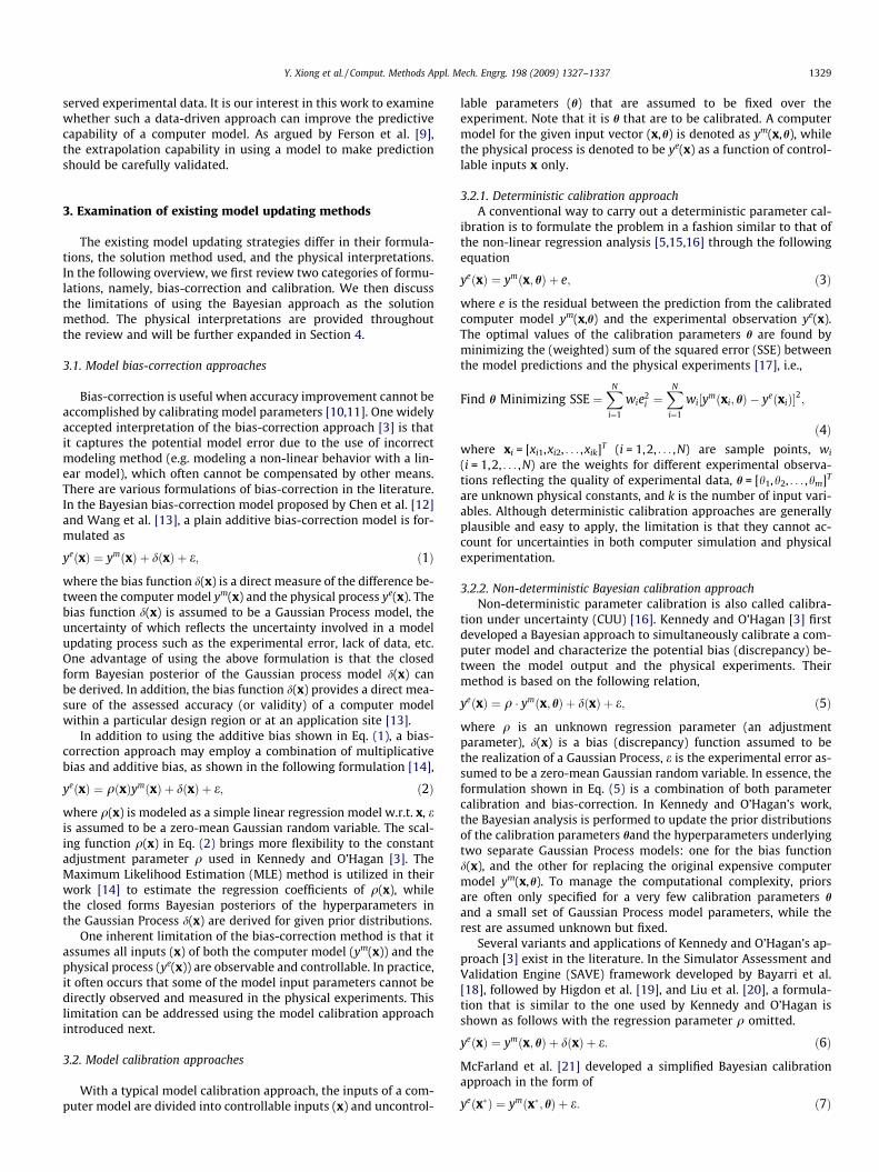
Fig. 1. Relationship of model updating, model refinement, and model validation.

1328 Y. Xiong et al. / Comput. Methods Appl. Mech. Engrg. 198 (2009) 1327–1337

calibration parameters are fixed and estimated, typically usingleast squares to match the model with the physical observations.This type of approach for model updating is inconsistent withthe primary concerns of model validation and prediction in whichvarious uncertainties should be accounted for either explicitly orimplicitly. Examples of such uncertainties include experimental er-ror, lack of data, uncertain model parameters, and model uncer-tainty (systematic model inadequacy). The more recent Bayesianstyle calibration, also named calibration under uncertainty (CUU)or stochastic calibration, treats calibration parameters as unknownentities that are fixed over the course of the physical experiment.Initial lack of knowledge of the parameters is represented byassigning prior distributions to them, and, given the experimentaldata, this lack of knowledge is revised by updating their distribu-tions (from priors to posteriors) based on the observed datathrough Bayesian analysis [3,4]. However, as we discuss in a morethorough examination in Section 3.2, several limitations of apply-ing the Bayesian calibration approaches are identified in this work.

One limitation of the aforementioned calibration approaches isthat the calibration parameters are assumed to remain fixed overthe entire course of the physical experiment and beyond. In con-trast, it is frequently the case that some parameters vary randomlyover the physical experiment, perhaps due to manufacturing vari-ation, variation in raw materials, variation in environmental orusage conditions, etc. This violates the assumptions under whichthe Bayesian or regression-based calibration analyses are derived.In this situation, rather than assuming fixed parameters and updat-ing their posterior distributions to represent our lack of knowledgeof them, it is more reasonable to treat them a randomly varyingand estimate their distributional properties by integrating thephysical data with the model. In essence, the distributional proper-ties (e.g. the mean and variance of the randomly varying parame-ters) become the calibration parameters for the model, and theobjective is to identify values for them that provide the best agree-ment with the observed distributional properties (e.g. the disper-sion [5]) of the physical experimental data. In this paper, wepresent a maximum likelihood estimation (MLE) [6] approach foraccomplishing this. The MLE method is used to estimate a set ofunknown parameters (heretofore called model updating parame-ters) associated with several modeling updating formulations,which include the distributional properties of parameters that varyrandomly over the experiment, as well as well as more traditionalfixed calibration parameters and quantities associated with bias-correction and random experimental error.

The remainder of the paper is organized as follows. In Section 2,we discuss the role that model updating plays versus model valida-tion and prediction. In Section 3, we examine the existing modelupdating formulations under two categories, namely, model bias-correction and calibration. The popular Bayesian approach isdescribed and its limitations are highlighted. In Section 4, we de-scribe our proposed MLE based model updating approach, togetherwith the introduction of the u-pooling validation metric. In Section5, a benchmark thermal challenge problem adopted by the SandiaValidation workshop [7,8] is used as an example to illustrate theproposed approach, draw important conclusions, and portray these

conclusions in relation to conclusions from prior studies. Section 6is the closure with a summary of the features of the proposedmethod, the relative merits of different approaches, the insightsgained, and future research directions.

2. Role of model updating vs. model validation

In this work, model updating is viewed as a process that contin-uously improves a computer model through mathematical meansbased on the results from newly added physical experiments, untilthe updated model satisfies the validation requirement or the re-source is exhausted. Therefore, even though model updating isinterrelated with model validation, it is viewed as a separate activ-ity that occurs before ‘‘validation”. As shown in Fig. 1, the modelupdating procedure integrates the computer simulation model ym

with the physical experiment data ye to yield an updated modelym0 ð�Þ. This updated model is then subject to a validation procedurethat utilizes additional physical experiments ye in the intended re-gion of interest for validation. As noted from this diagram, unlikemany contemporary model validation works, model validation inthis work is used to evaluate an evolved, updated model ym0 ð�Þ,rather than the original computer model ym(�). Besides, the up-dated model ym0 ð�Þ is the one used for making future predictionypred(�) with the consideration of various sources of uncertainties.For implementing model updating and validation in a computa-tionally efficient manner, it is indicated in Fig. 1 that a metamodel(surrounded by a dashed box) may be used to substitute the origi-nal computer model if it is expensive to compute.

As more details are provided in the remaining sections,modelupdating utilizes mathematical means (e.g. calibrating modelparameters, bias-correction) to match model predictions with thephysical observations. Model updating provides not only the for-mulation of an updated model, but also the characterization ofmodel updating parameters H, together with the associatedassumptions. As noted, the model updating procedure, duringwhich ym(�) is treated as a black-box, is largely driven by the ob-

Y. Xiong et al. / Comput. Methods Appl. Mech. Engrg. 198 (2009) 1327–1337 1329

served experimental data. It is our interest in this work to examinewhether such a data-driven approach can improve the predictivecapability of a computer model. As argued by Ferson et al. [9],the extrapolation capability in using a model to make predictionshould be carefully validated.

3. Examination of existing model updating methods

The existing model updating strategies differ in their formula-tions, the solution method used, and the physical interpretations.In the following overview, we first review two categories of formu-lations, namely, bias-correction and calibration. We then discussthe limitations of using the Bayesian approach as the solutionmethod. The physical interpretations are provided throughoutthe review and will be further expanded in Section 4.

3.1. Model bias-correction approaches

Bias-correction is useful when accuracy improvement cannot beaccomplished by calibrating model parameters [10,11]. One widelyaccepted interpretation of the bias-correction approach [3] is thatit captures the potential model error due to the use of incorrectmodeling method (e.g. modeling a non-linear behavior with a lin-ear model), which often cannot be compensated by other means.There are various formulations of bias-correction in the literature.In the Bayesian bias-correction model proposed by Chen et al. [12]and Wang et al. [13], a plain additive bias-correction model is for-mulated as

yeðxÞ ¼ ymðxÞ þ dðxÞ þ e; ð1Þ

where the bias function d(x) is a direct measure of the difference be-tween the computer model ym(x) and the physical process ye(x). Thebias function d(x) is assumed to be a Gaussian Process model, theuncertainty of which reflects the uncertainty involved in a modelupdating process such as the experimental error, lack of data, etc.One advantage of using the above formulation is that the closedform Bayesian posterior of the Gaussian process model d(x) canbe derived. In addition, the bias function d(x) provides a direct mea-sure of the assessed accuracy (or validity) of a computer modelwithin a particular design region or at an application site [13].

In addition to using the additive bias shown in Eq. (1), a bias-correction approach may employ a combination of multiplicativebias and additive bias, as shown in the following formulation [14],

yeðxÞ ¼ qðxÞymðxÞ þ dðxÞ þ e; ð2Þ

where q(x) is modeled as a simple linear regression model w.r.t. x, eis assumed to be a zero-mean Gaussian random variable. The scal-ing function q(x) in Eq. (2) brings more flexibility to the constantadjustment parameter q used in Kennedy and O’Hagan [3]. TheMaximum Likelihood Estimation (MLE) method is utilized in theirwork [14] to estimate the regression coefficients of q(x), whilethe closed forms Bayesian posteriors of the hyperparameters inthe Gaussian Process d(x) are derived for given prior distributions.

One inherent limitation of the bias-correction method is that itassumes all inputs (x) of both the computer model (ym(x)) and thephysical process (ye(x)) are observable and controllable. In practice,it often occurs that some of the model input parameters cannot bedirectly observed and measured in the physical experiments. Thislimitation can be addressed using the model calibration approachintroduced next.

3.2. Model calibration approaches

With a typical model calibration approach, the inputs of a com-puter model are divided into controllable inputs (x) and uncontrol-

lable parameters (h) that are assumed to be fixed over theexperiment. Note that it is h that are to be calibrated. A computermodel for the given input vector (x,h) is denoted as ym(x,h), whilethe physical process is denoted to be ye(x) as a function of control-lable inputs x only.

3.2.1. Deterministic calibration approachA conventional way to carry out a deterministic parameter cal-

ibration is to formulate the problem in a fashion similar to that ofthe non-linear regression analysis [5,15,16] through the followingequation

yeðxÞ ¼ ymðx; hÞ þ e; ð3Þ

where e is the residual between the prediction from the calibratedcomputer model ym(x,h) and the experimental observation ye(x).The optimal values of the calibration parameters h are found byminimizing the (weighted) sum of the squared error (SSE) betweenthe model predictions and the physical experiments [17], i.e.,

Find h Minimizing SSE ¼XN

i¼1

wie2i ¼

XN

i¼1

wi½ymðxi; hÞ � yeðxiÞ�2;

ð4Þwhere xi = [xi1,xi2, . . . ,xik]T (i = 1,2, . . . ,N) are sample points, wi

(i = 1,2, . . . ,N) are the weights for different experimental observa-tions reflecting the quality of experimental data, h = [h1,h2, . . . ,hm]T

are unknown physical constants, and k is the number of input vari-ables. Although deterministic calibration approaches are generallyplausible and easy to apply, the limitation is that they cannot ac-count for uncertainties in both computer simulation and physicalexperimentation.

3.2.2. Non-deterministic Bayesian calibration approachNon-deterministic parameter calibration is also called calibra-

tion under uncertainty (CUU) [16]. Kennedy and O’Hagan [3] firstdeveloped a Bayesian approach to simultaneously calibrate a com-puter model and characterize the potential bias (discrepancy) be-tween the model output and the physical experiments. Theirmethod is based on the following relation,

yeðxÞ ¼ q � ymðx; hÞ þ dðxÞ þ e; ð5Þ

where q is an unknown regression parameter (an adjustmentparameter), d(x) is a bias (discrepancy) function assumed to bethe realization of a Gaussian Process, e is the experimental error as-sumed to be a zero-mean Gaussian random variable. In essence, theformulation shown in Eq. (5) is a combination of both parametercalibration and bias-correction. In Kennedy and O’Hagan’s work,the Bayesian analysis is performed to update the prior distributionsof the calibration parameters hand the hyperparameters underlyingtwo separate Gaussian Process models: one for the bias functiond(x), and the other for replacing the original expensive computermodel ym(x,h). To manage the computational complexity, priorsare often only specified for a very few calibration parameters h

and a small set of Gaussian Process model parameters, while therest are assumed unknown but fixed.

Several variants and applications of Kennedy and O’Hagan’s ap-proach [3] exist in the literature. In the Simulator Assessment andValidation Engine (SAVE) framework developed by Bayarri et al.[18], followed by Higdon et al. [19], and Liu et al. [20], a formula-tion that is similar to the one used by Kennedy and O’Hagan isshown as follows with the regression parameter q omitted.

yeðxÞ ¼ ymðx; hÞ þ dðxÞ þ e: ð6Þ

McFarland et al. [21] developed a simplified Bayesian calibrationapproach in the form of

yeðx�Þ ¼ ymðx�; hÞ þ e: ð7Þ


Their method does not consider the bias-correction, and poses theprior belief of the calibration parameters h as uniformly distributed.Unlike others, their calibration is only performed at one particularsite x*, based on the assumption that the results of calibration areidentical at different input sites. Such an assumption is question-able if the computer model is so wrong that the calibration at onesingle site could be heavily biased and is hard to be extrapolatedto other sites.

3.3. Limitations of Bayesian approaches

While the Bayesian approach is useful when limited data areavailable, there are several common issues. First, as indicated inTrucano et al. [16], the prior distributions of calibration parametersare often difficult to specify due to the lack of prior knowledge.Subjectively assigned prior distributions may yield unstable pos-terior distributions [22], which undermines the advantage ofBayesian updating. Second, the Markov Chain Monte Carlo (MCMC)method used in most Bayesian calibration practices for obtainingthe posterior distributions requires a significant amount of itera-tions, while the criterion for ceasing the Markov Chain growth isnot established [16].

Loeppky et al. [23] examined a non-Bayesian version of theapproach from Kennedy and O’Hagan [3], but using the MLE toestimate the calibration parameters which are assumed determin-istic. The issue of identifiability of model bias was addressed byexamining the likelihood ratio of two model versions: one withthe bias term, the other without. It was demonstrated that theMLE estimates of calibration parameters will asymptotically attainan unbiased computer model if such a model exists. However, theirmethod provides deterministic MLE estimates without acknowl-edging the uncertainty of model input.

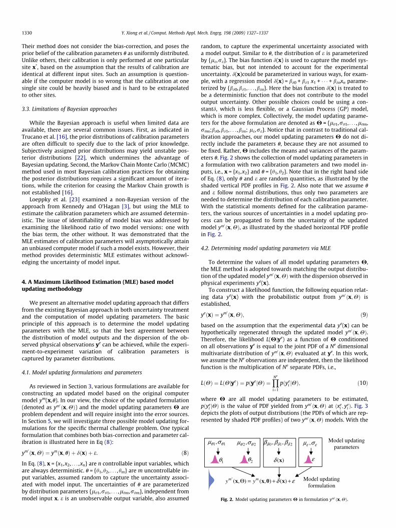
Fig. 2. Model updating parameters H in formulation ym0 ðx;HÞ.

4. A Maximum Likelihood Estimation (MLE) based modelupdating methodology

We present an alternative model updating approach that differsfrom the existing Bayesian approach in both uncertainty treatmentand the computation of model updating parameters. The basicprinciple of this approach is to determine the model updatingparameters with the MLE, so that the best agreement betweenthe distribution of model outputs and the dispersion of the ob-served physical observations ye can be achieved, while the experi-ment-to-experiment variation of calibration parameters iscaptured by parameter distributions.

4.1. Model updating formulations and parameters

As reviewed in Section 3, various formulations are available forconstructing an updated model based on the original computermodel ym(x,h). In our view, the choice of the updated formulation(denoted as ym0 ðx;HÞ) and the model updating parameters H areproblem dependent and will require insight into the error sources.In Section 5, we will investigate three possible model updating for-mulations for the specific thermal challenge problem. One typicalformulation that combines both bias-correction and parameter cal-ibration is illustrated here in Eq (8):

ym0 ðx;HÞ ¼ ymðx; hÞ þ dðxÞ þ e: ð8Þ

In Eq. (8), x = {x1,x2, . . . ,xn} are n controllable input variables, whichare always deterministic. h = {h1,h2, . . . ,hm} are m uncontrollable in-put variables, assumed random to capture the uncertainty associ-ated with model input. The uncertainties of h are parameterizedby distribution parameters {lh1,rh1, . . . ,lhm,rhm}, independent frommodel input x. e is an unobservable output variable, also assumed

random, to capture the experimental uncertainty associated witha model output. Similar to h, the distribution of e is parameterizedby {le,re}. The bias function d(x) is used to capture the model sys-tematic bias, but not intended to account for the experimentaluncertainty. d(x)could be parameterized in various ways, for exam-ple, with a regression model d(x) = bd0 + bd1 x1 + � � � + bdnxn parame-terized by {bd0,bd1, . . . ,bdn}. Here the bias function d(x) is treated tobe a deterministic function that does not contribute to the modeloutput uncertainty. Other possible choices could be using a con-stantd, which is less flexible, or a Gaussian Process (GP) model,which is more complex. Collectively, the model updating parame-ters for the above formulation are denoted as H = {lh1,rh1, . . . ,lhm,rhm;bd0,bd1, . . . ,bdn; le,re}. Notice that in contrast to traditional cal-ibration approaches, our model updating parameters H do not di-rectly include the parameters h, because they are not assumed tobe fixed. Rather, H includes the means and variances of the param-eters h. Fig. 2 shows the collection of model updating parameters ina formulation with two calibration parameters and two model in-puts, i.e., x = {x1,x2} and h = {h1,h2}. Note that in the right hand sideof Eq. (8), only h and e are random quantities, as illustrated by theshaded vertical PDF profiles in Fig. 2. Also note that we assume h

and e follow normal distributions, thus only two parameters areneeded to determine the distribution of each calibration parameter.With the statistical moments defined for the calibration parame-ters, the various sources of uncertainties in a model updating pro-cess can be propagated to form the uncertainty of the updatedmodel ym0 ðx;HÞ, as illustrated by the shaded horizontal PDF profilein Fig. 2.

4.2. Determining model updating parameters via MLE

To determine the values of all model updating parameters H,the MLE method is adopted towards matching the output distribu-tion of the updated model ym0 ðx;HÞwith the dispersion observed inphysical experiments ye(x).

To construct a likelihood function, the following equation relat-ing data ye(x) with the probabilistic output from ym0 ðx;HÞ isestablished,

yeðxÞ ¼ ym0 ðx;HÞ; ð9Þ

based on the assumption that the experimental data ye(x) can behypothetically regenerated through the updated model ym0 ðx;HÞ.Therefore, the likelihood L(Hjye) as a function of H conditionedon all observations ye is equal to the joint PDF of a Ne dimensionalmultivariate distribution of ym0 ðx;HÞ evaluated at ye. In this work,we assume the Ne observations are independent, then the likelihoodfunction is the multiplication of Ne separate PDFs, i.e.,

LðHÞ ¼ LðHjyeÞ ¼ pðyejHÞ ¼YNe

i¼1

pðyei jHÞ; ð10Þ

where H are all model updating parameters to be estimated,pðye

i jHÞ is the value of PDF yielded from ym0 ðx;HÞ at ðxei ; y

ei Þ. Fig. 3

depicts the plots of output distributions (the PDFs of which are rep-resented by shaded PDF profiles) of two ym0 ðx;HÞ models. With the

x

ey

'my

x

ey

'my

Physical experiment

Distribution of

ey

'my

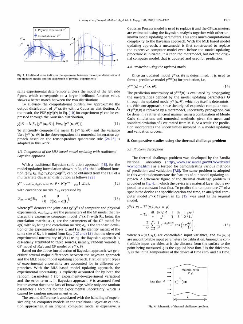
Fig. 3. Likelihood value indicates the agreement between the output distribution ofthe updated model and the dispersion of physical experiments.

Fig. 4. Schematic of thermal challenge problem.


same experimental data (empty circles), the model of the left sidefigure, which corresponds to a larger likelihood function value,shows a better match between the two distributions.

To alleviate the computational burden, we approximate theoutput distribution of ym0 ðx;HÞ with a Gaussian distribution. Asthe result, the PDF pðye

i jHÞ in Eq. (10) for experiment yei can be ex-

pressed through the Gaussian distribution,

yei jH � NðEHfym0 ðxi;HÞg;VarHfym0 ðxi;HÞgÞ: ð11Þ

To efficiently compute the mean EHfym0 ðxi;HÞg and the varianceVarHfym0 ðxi;HÞ in the above equation, the numerical integration ap-proach based on the tensor-product quadrature rule [24,25] isadopted in this work.

4.3. Comparison of the MLE based model updating with traditionalBayesian approach

With a traditional Bayesian calibration approach [18], for themodel updating formulation shown in Eq. (6), the likelihood func-tion L(rm,rm,lm;rd,rd;re;hjyem) can be obtained from the PDF of amultivariate Gaussian distribution as follows [23]

yemjrm; rm;lm; rd; rd;re; h � Nðyem � lm1;RemÞ; ð12Þ

with covariance matrix Rem expressed by

Rem ¼ r2mRm þ

0 00 r2

d Rd þ r2e I

� �; ð13Þ

where yem denotes the joint data (ye,ym) of computer and physicalexperiments, rm,rm,lm are the parameters of the GP model that re-places the expensive computer model ym(x,h) with Rm being thecorrelation matrix; rd,rd are the parameters of the GP model ford(x) with Rd being the correlation matrix; re is the standard devia-tion of the experimental error e; and I is the identity matrix of thesame size of Rd. It is noted from Eqs. (12) and (13) that the observedexperimental uncertainty of ye(x) using the Bayesian approach isessentially attributed to three sources, namely, random variable e,GP model of d(x), and GP model of ym(x,h).

Based on the above introduction of Bayesian approach, we gen-eralize several major differences between the Bayesian approachand the MLE based model updating approach. First, different typesof experimental uncertainty are accounted for in different ap-proaches. With the MLE based model updating approach, theexperimental uncertainty is explicitly accounted for by both therandom parameters h (for experiment-to-experiment variation)and the error term e. In Bayesian approach, h is assumed fixedbut unknown due to the lack of knowledge, while only one randomparameter e accounts for the experimental uncertainty, which iscaused by random measurement error.

The second difference is associated with the handling of expen-sive original computer models. In the traditional Bayesian calibra-tion approaches, if an original computer model is expensive, a

Gaussian Process model is used to replace it and the GP parametersare estimated using the Bayesian analysis together with other un-known model updating parameters. This adds much computationalcomplexity to the Bayesian approach. With the MLE based modelupdating approach, a metamodel is first constructed to replacethe expensive computer model even before the model updatingprocedure is initiated. It is then the metamodel, but not the origi-nal computer model, that is updated and used for prediction.

4.4. Prediction using the updated model

Once an updated model ym0 ðx;HÞ is determined, it is used toform a predictive model ypred(x) for prediction, i.e.,

ypredðxÞ ¼ ym0 ðx;HÞ: ð14Þ

The prediction uncertainty of ypred(x) is evaluated by propagatingthe uncertainties defined by the model updating parameters Hthrough the updated model ym0 ðx;HÞ, which by itself is determinis-tic. With our approach, since the original expensive computer mod-el ym(x,h) is replaced by a metamodel, uncertainty propagation canbe done in a rather efficient manner using a combination of MonteCarlo simulations and numerical methods, given the mean andstandard deviation of h estimated from MLE. As a result, the predic-tion incorporates the uncertainties involved in a model updatingand validation process.

5. Comparative studies using the thermal challenge problem

5.1. Problem description

The thermal challenge problem was developed by the SandiaNational Laboratory (http://www.esc.sandia.gov/VCWwebsite/vcwhome.html) as a testbed for demonstrating various methodsof prediction and validation [7,8]. The same problem is adoptedin this work to demonstrate the features of our model updating ap-proach. A schematic figure of the thermal challenge problem isprovided in Fig. 4, in which the device is a material layer that is ex-posed to a constant heat flux. To predict the temperature Tm of aspot in the device at a specific location and time, an analytical com-puter model ym(x,h) given in Eq. (15) was used as the originalmodel.

ymðx; hÞ ¼ Tmðq; L; xl; t;j;qÞ

¼ T0 þqLjðj=qÞt

L2 þ 13� xl

Lþ 1

2xl

L

� �2�

� 2p2

X6

n¼1

1n2 e�n2p2 ðj=qÞt

L2 cos np xl

L

� �#; ð15Þ

where x = (q,L,xl, t) are controllable input variables, and h = (j,q)are uncontrollable input parameters for calibration. Among the con-trollable input variables, xl is the distance from the surface to thepoint being measured, q is the applied heat flux, L is the thickness,T0 is the initial temperature of the device at time zero, and t is time.

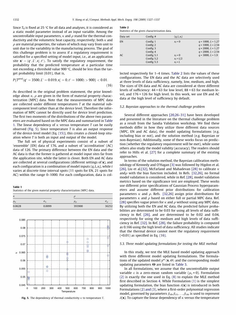
http://www.esc.sandia.gov/VCWwebsite/vcwhome.html

http://www.esc.sandia.gov/VCWwebsite/vcwhome.html

Table 2Statistics of the given characterization data.

Data set Config # (q,L,xl)

EN Config 1 xl = 0 q = 1000, L = 1.27Config 2 q = 1000, L = 2.54Config 3 q = 2000, L = 1.27Config 4 q = 2000, L = 2.54

AC Config 5.1 xl = 0 q = 3000, L = 1.9Config 5.2 xl = L/2Config 5.3 xl = L


Since T0 is fixed at 25 �C for all data and analyses, it is considered asa static model parameter instead of an input variable. Among theuncontrollable input parameters, j and q stand for the thermal con-ductivity and the volumetric heat capacity, respectively; both j andq are material properties, the values of which may vary from unit tounit due to the variability in the manufacturing process. The goal ofthis challenge problem is to assess if a regulatory requirement issatisfied for a specified setting of model input, i.e., at an applicationsite x� ¼ ðq�; L�; x�l ; t�Þ. To satisfy the regulatory requirement, theprobability that the predicted temperature at a particular timenot exceeding a threshold value 900 �C, should be less than the tar-get probability limit (0.01), that is,

PfTpredðq� ¼ 3500; L� ¼ 0:019; x�l ¼ 0; t� ¼ 1000Þ > 900g < 0:01:

ð16Þ

As described in the original problem statement, the prior knowl-edge about j, q are given in the form of material property charac-terization (MPC) data. Note that the measurements of MPC dataare collected under different temperatures T at the material sub-component level rather than at the device level. Therefore the infor-mation of MPC cannot be directly used for device level prediction.The first two moments of the distributions of the above two param-eters are evaluated based on the MPC data and summarized in Table1. The linear dependency of j versus temperature T can be easilyobserved (Fig. 5). Since temperature T is also an output responseof the device-level model (Eq. (15)), this creates a closed-loop situ-ation where T is both an input and output of the model.

The full set of physical experiments consist of a subset of‘ensemble’ (EN) data of 176, and a subset of ‘accreditation’ (AC)data of 126. The primary difference between the EN data and theAC data is that the former is gathered at model input sites far fromthe application site, while the latter is closer. Both EN and AC dataare collected at several configurations (different settings of x), andeach configuration is a combination of model inputs (q,L,xl), while tvaries at discrete time interval spots (11 spots for EN, 21 spots forAC) within the range 0–1000. For each configuration, data is col-

Table 1Statistics of the given material property characterization (MPC) data.

j q

lj rj lq rq

0.0628 0.0099 393900 36252

0 100 200 300 400 500 600 700 800 900 10000.045

0.05

0.055

0.06

0.065

0.07

0.075

0.08

0.085

Temperature

k

Fig. 5. The dependency of thermal conductivity j to temperature T.

lected respectively for 1–4 times. Table 2 lists the values of theseconfigurations. The EN data and the AC data are selectively usedat three levels of data sufficiency, namely, low, medium, and high.The sizes of EN data and AC data are considered at three differentlevels of sufficiency: 44 + 63 for low level, 88 + 63 for medium le-vel, and 176 + 126 for high level. In this work, we use EN and ACdata at the high level of sufficiency by default.

5.2. Bayesian approaches to the thermal challenge problem

Several different approaches [20,26–31] have been developedand presented in the literature on the thermal challenge problemas a result from the Sandia Validation workshop. We find thesemethods differ in how they utilize three different data sources(MPC, EN and AC data), the model updating formulations (e.g.including bias or not), and the solution method (e.g. Bayesian ornon-Bayesian). Additionally, some of these works focus on predic-tion (whether the regulatory requirement will be met), while someothers also study the model validity (accuracy). The readers shouldrefer to Hills et al. [27] for a complete summary of the existingapproaches.

In terms of the solution method, the Bayesian calibration meth-odology of Kennedy and O’Hagan [3] was followed by Higdon et al.[26], Liu et al.[32], McFarland and Mahadevan [28] to calibrate jandq with the bias function included. In Refs. [32,26], no formalmodel validation is considered, while in Ref. [28], model validationmetrics based on the significance test are employed. These worksuse different prior specifications of Gaussian Process hyperparam-eters and assume different prior distributions for calibrationparameters j and q. Refs. [32,26] assign prior distributions forparameters j and q based on either full or partial MPC data. Ref.[28] specifies vague priors for j and q without using any MPC data.By utilizing both the EN and AC data, the predicted failure proba-bilities are determined to be 0.03 for using all levels of data suffi-ciency in Ref. [26], and are determined to be 0.02 and 0.04,respectively for using the medium and high levels of data suffi-ciency in Ref. [32]. In Ref. [28], the failure probability is computedas 0.166 using the high level of data sufficiency. All studies indicatethat the thermal device cannot meet the regulatory requirement(<0.01) as specified in Eq. (16).

5.3. Three model updating formulations for testing the MLE method

In this study, we test the MLE based model updating approachwith three different model updating formulations. The formula-tions of the updated model ym0 ðx;HÞ and the corresponding modelupdating parameters H are listed in Table 3.

In all formulations, we assume that the uncontrollable outputvariable e is a zero-mean random variable (le = 0). Formulation(2) is exactly the one used in Eq. (8) to explain the MLE methodfirst described in Section 4. While Formulation (1) is the simplestupdating formulation, the bias function d(x) is introduced in bothFormulations (2) and (3), where a first-order polynomial regressionmodel, governed by parameters bd0,bd1, . . . ,bd4, is used to representd(x). To capture the linear dependency of j versus the temperature

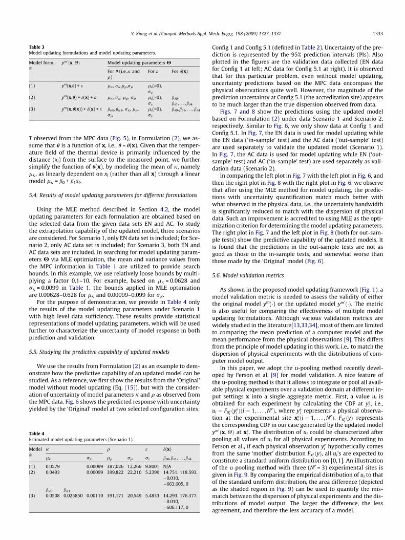
Table 3Model updating formulations and model updating parameters.

Model form.#

ym0 ðx;HÞ Model updating parameters H

For h (i.e.,j andq)

For e For d(x)

(1) ym(x,h) + e lj, rj,lq,rq le(=0),re

(2) ym(x,h) + d(x) + e lj, rj, lq, rq le(=0),re

bd0,bd1, . . . ,bd4

(3) ym(x,h(x)) + d(x) + e bj0,bj1, rj, lq,rq

le(=0),re

bd0,bd1, . . . ,bd4


T observed from the MPC data (Fig. 5), in Formulation (2), we as-sume that h is a function of x, i.e., h = h(x). Given that the temper-ature field of the thermal device is primarily influenced by thedistance (xl) from the surface to the measured point, we furthersimplify the function of h(x), by modeling the mean of j, namelylj, as linearly dependent on xl (rather than all x) through a linearmodel lj = b0 + b1xl.

5.4. Results of model updating parameters for different formulations

Using the MLE method described in Section 4.2, the modelupdating parameters for each formulation are obtained based onthe selected data from the given data sets EN and AC. To studythe extrapolation capability of the updated model, three scenariosare considered. For Scenario 1, only EN data set is included; for Sce-nario 2, only AC data set is included; For Scenario 3, both EN andAC data sets are included. In searching for model updating param-eters H via MLE optimiation, the mean and variance values fromthe MPC information in Table 1 are utilized to provide searchbounds. In this example, we use relatively loose bounds by multi-plying a factor 0.1–10. For example, based on lj = 0.0628 andrj = 0.0099 in Table 1, the bounds applied in MLE optimiationare 0.00628–0.628 for lj and 0.00099–0.099 for rj.

For the purpose of demonstration, we provide in Table 4 onlythe results of the model updating parameters under Scenario 1with high level data sufficiency. These results provide statisticalrepresentations of model updating parameters, which will be usedfurther to characterize the uncertainty of model response in bothprediction and validation.

5.5. Studying the predictive capability of updated models

We use the results from Formulation (2) as an example to dem-onstrate how the predictive capability of an updated model can bestudied. As a reference, we first show the results from the ‘Original’model without model updating (Eq. (15)), but with the consider-ation of uncertainty of model parameters j and q as observed fromthe MPC data. Fig. 6 shows the predicted response with uncertaintyyielded by the ‘Original’ model at two selected configuration sites:

Table 4Estimated model updating parameters (Scenario 1).

Model#

j q e d(x)

lj rj lq rq re bd0,bd1, . . . ,bd4

(1) 0.0579 0.00099 387,026 12,266 9.8001 N/A(2) 0.0493 0.00099 399,822 22,210 5.2399 14.751, 118.593,

�0.010,�663.605, 0

bj0 bj1

(3) 0.0508 0.025850 0.00110 391,171 20,549 5.4833 14.293, 176.377,�0.010,�606.117, 0

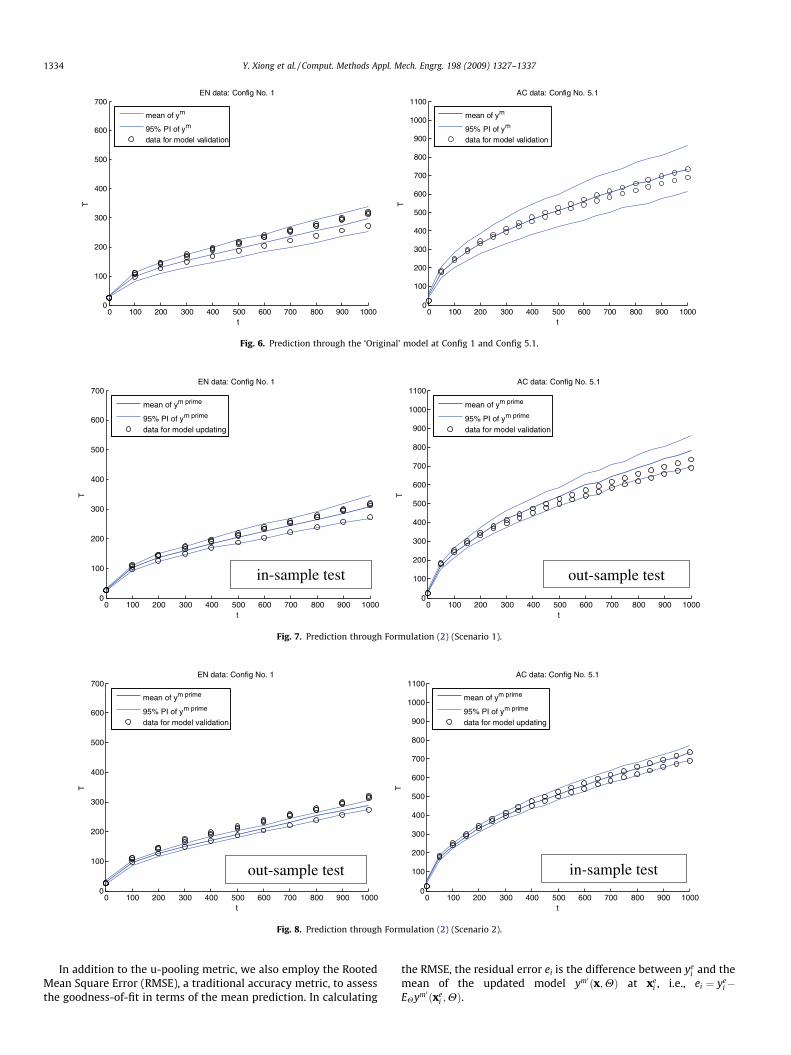
Config 1 and Config 5.1 (defined in Table 2). Uncertainty of the pre-diction is represented by the 95% prediction intervals (PIs). Alsoplotted in the figures are the validation data collected (EN datafor Config 1 at left; AC data for Config 5.1 at right). It is observedthat for this particular problem, even without model updating,uncertainty predictions based on the MPC data encompass thephysical observations quite well. However, the magnitude of theprediction uncertainty at Config 5.1 (the accreditation site) appearsto be much larger than the true dispersion observed from data.

Figs. 7 and 8 show the predictions using the updated modelbased on Formulation (2) under data Scenario 1 and Scenario 2,respectively. Similar to Fig. 6, we only show data at Config 1 andConfig 5.1. In Fig. 7, the EN data is used for model updating whilethe EN data (‘in-sample’ test) and the AC data (‘out-sample’ test)are used separately to validate the updated model (Scenario 1).In Fig. 7, the AC data is used for model updating while EN (‘out-sample’ test) and AC (‘in-sample’ test) are used separately as vali-dation data (Scenario 2).

In comparing the left plot in Fig. 7 with the left plot in Fig. 6, andthen the right plot in Fig. 8 with the right plot in Fig. 6, we observethat after using the MLE method for model updating, the predic-tions with uncertainty quantification match much better withwhat observed in the physical data, i.e., the uncertainty bandwidthis significantly reduced to match with the dispersion of physicaldata. Such an improvement is accredited to using MLE as the opti-mization criterion for determining the model updating parameters.The right plot in Fig. 7 and the left plot in Fig. 8 (both for out-sam-ple tests) show the predictive capability of the updated models. Itis found that the predictions in the out-sample tests are not asgood as those in the in-sample tests, and somewhat worse thanthose made by the ‘Original’ model (Fig. 6).

5.6. Model validation metrics

As shown in the proposed model updating framework (Fig. 1), amodel validation metric is needed to assess the validity of eitherthe original model ym(�) or the updated model ym0 ð�Þ. The metricis also useful for comparing the effectiveness of multiple modelupdating formulations. Although various validation metrics arewidely studied in the literature[13,33,34], most of them are limitedto comparing the mean prediction of a computer model and themean performance from the physical observations [9]. This differsfrom the principle of model updating in this work, i.e., to match thedispersion of physical experiments with the distributions of com-puter model output.

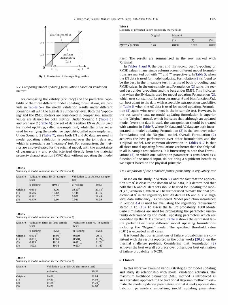
In this paper, we adopt the u-pooling method recently devel-oped by Ferson et al. [9] for model validation. A nice feature ofthe u-pooling method is that it allows to integrate or pool all avail-able physical experiments over a validation domain at different in-put settings x into a single aggregate metric. First, a value ui isobtained for each experiment by calculating the CDF at ye

i , i.e.,ui ¼ Fxe

iðye

i Þði ¼ 1; . . . ;NeÞ, where yei represents a physical observa-

tion at the experimental site xei ði ¼ 1; . . . ;NeÞ. Fxe

iðyÞ represents

the corresponding CDF in our case generated by the updated modelym0 ðx;HÞ at xe

i . The distribution of ui could be characterized afterpooling all values of ui for all physical experiments. According toFerson et al., if each physical observation ye

i hypothetically comesfrom the same ‘mother’ distribution Fxe

iðyÞ, all ui’s are expected to

constitute a standard uniform distribution on [0,1]. An illustrationof the u-pooling method with three (Ne = 3) experimental sites isgiven in Fig. 9. By comparing the empirical distribution of ui to thatof the standard uniform distribution, the area difference (depictedas the shaded region in Fig. 9) can be used to quantify the mis-match between the dispersion of physical experiments and the dis-tributions of model output. The larger the difference, the lessagreement, and therefore the less accuracy of a model.

0 100 200 300 400 500 600 700 800 900 10000

100

200

300

400

500

600

700EN data: Config No. 1

t

T

mean of ym

95% PI of ym

data for model validation

0 100 200 300 400 500 600 700 800 900 10000

100

200

300

400

500

600

700

800

900

1000

1100AC data: Config No. 5.1

t

T

mean of ym

95% PI of ym


Fig. 6. Prediction through the ‘Original’ model at Config 1 and Config 5.1.

0 100 200 300 400 500 600 700 800 900 10000

100

200

300

400

500

600


t

T

mean of ym prime

95% PI of ym prime

data for model updating

0 100 200 300 400 500 600 700 800 900 10000

100

200

300

400

500

600

700

800

900

1000


t

Tmean of ym prime

95% PI of ym prime


out-sample testin-sample test

Fig. 7. Prediction through Formulation (2) (Scenario 1).

0 100 200 300 400 500 600 700 800 900 10000

100

200

300

400

500

600


t

T

mean of ym prime

95% PI of ym prime


0 100 200 300 400 500 600 700 800 900 10000

100

200

300

400

500

600

700

800

900

1000


t

T

mean of ym prime

95% PI of ym prime

data for model updating

in-sample test out-sample test

Fig. 8. Prediction through Formulation (2) (Scenario 2).


In addition to the u-pooling metric, we also employ the RootedMean Square Error (RMSE), a traditional accuracy metric, to assessthe goodness-of-fit in terms of the mean prediction. In calculating

the RMSE, the residual error ei is the difference between yei and the

mean of the updated model ym0 ðx;HÞ at xei , i.e., ei ¼ ye

i�EHym0 ðxe

i ;HÞ.

1u0 u

uniform distribution

(0,1)

3u2u

1/3

2/3

1

1

distribution of iu

Fig. 9. Illustration of the u-pooling method.

Table 8Summary of predicted failure probability (Scenario 3).

Original Model #

(1) (2) (3)

P{Tpred(x*) > 900} 0.26 0.060 0.028 0.092


5.7. Comparing model updating formulations based on validationmetrics

For comparing the validity (accuracy) and the predictive capa-bility of the three different model updating formulations, we pro-vide in Tables 5–7 the model validation results under differentscenarios, all with the high data sufficiency level. Both the ‘u-pool-ing’ and the RMSE metrics are considered in comparison; smallervalues are desired for both metrics. Under Scenario 1 (Table 5)and Scenario 2 (Table 6), one set of data (either EN or AC) is usedfor model updating, called in-sample test; while the other set isused for verifying the predictive capability, called out-sample test.Under Scenario 3 (Table 7), since both EN and AC data are used inmodel updating, validation is performed over the joint data set,which is essentially an ‘in-sample’ test. For comparison, the met-rics are also evaluated for the original model, with the uncertaintyof parameters j and q characterized directly from the materialproperty characterization (MPC) data without updating the model

Table 5Summary of model validation metrics (Scenario 1).

Model # Validation data: EN (in-sampletest)

Validation data: AC (out-sampletest)

u-Pooling RMSE u-Pooling RMSE

Original 0.634 16.96 0.830** 29.13*

(1) 0.566 15.12* 1.138 33.36(2) 0.521** 15.07** 0.901* 19.43**

(3) 0.579 15.16 1.041 31.39


Model # Validation data: EN (out-sampletest)

Validation data: AC (in-sampletest)

u-Pooling RMSE u-Pooling RMSE

Original 0.634** 16.96** 0.830 29.13(1) 0.891 17.87* 0.540 11.27*

(2) 0.813* 18.14 0.471* 11.24**

(3) 1.002 19.53 0.463** 11.40


Model # Validation data: EN + AC (in-sample test)

u-Pooling RMSE

Original 0.456 22.84(1) 0.420* 14.98(2) 0.388** 14.29**

(3) 0.429 14.60*

itself. The results are summarized in the row marked with‘Original’.

In Tables 5 and 6, the best and the second best ‘u-pooling’ orRMSE values in any single column across different model formula-tions are marked out with ‘**’ and ‘*’ respectively. In Table 5, whenthe EN data is used for model updating, Formulation (2) is found tobe the best in the in-sample test in terms of both ‘u-pooling’ andRMSE values. In the out-sample test, Formulation (2) ranks the sec-ond best under ‘u-pooling’ and the best under RMSE. This indicatesthat when the EN data is used for model updating, Formulation (2),which uses constant calibration parameter h and bias function d(x),can best adapt to the data with acceptable extrapolation capability.In Table 6, when the AC data is used for model updating, Formula-tion (2) again wins over others in the in-sample test. However, inthe out-sample test, no model updating formulation is superiorto the ‘Original’ model, which indicates that, although an updatedmodel favors the data it used, the extrapolation should be treatedwith caution. In Table 7, where EN data and AC data are both incor-porated in model updating, Formulation (2) is the best over otherformulations and the ‘Original’ model. Overall, Formulation (2)achieves the best performance over other formulations and the‘Original’ model. One common observation in Tables 5–7 is thatall three model updating formulations are better than the ‘Original’in all in-sample test columns. It is interesting to note that Formu-lations (3), in which one calibration parameter is considered as afunction of one model input, do not bring a significant benefit aswe expect based on the physical principle.

5.8. Comparison of the predicted failure probability in regulatory test

Based on the study in Section 5.7 and the fact that the applica-tion site x* is close to the domain of AC data, it is determined thatboth the EN and AC data sets should be used for updating the mod-el (i.e., Scenario 3) which will be further used to make the final pre-diction at x* in the regulatory test. All data in EN and AC (i.e., highlevel data sufficiency) is considered. Model prediction introducedin Section 4.4 is used for evaluating the regulatory requirementstated in Eq. (16). To assess the failure probability, 1000 MonteCarlo simulations are used for propagating the parameter uncer-tainty determined by the model updating parameters which areidentified by the MLE approach. Table 8 shows the estimated fail-ure probabilities using different model updating formulationsincluding the ‘Original’ model. The specified threshold value(0.01) is exceeded in all cases.

It is found that our estimations of failure probabilities are con-sistent with the results reported in the other works [20,26] on thethermal challenge problem. Considering that Formulation (2)achieves the best overall accuracy over others, our best estimationof failure probability is 0.028.

6. Closure

In this work we examine various strategies for model updatingand study its relationship with model validation activities. Themaximum likelihood estimation (MLE) method is introduced asan alternative approach to the traditional Bayesian method to esti-mate the model updating parameters, so that it seeks optimal dis-tribution parameters underlying model updating parameters


through MLE. Unlike the traditional Bayesian approach which treatscalibration parameters as fixed but unknown due to lack of knowl-edge, the MLE based approach treats calibration parameters asintrinsic random to account for the uncertainty due to experi-ment-to-experiment variability. Other differences of the two meth-ods are summarized in Section 4.3 and will not be repeated here.

Through the thermal challenge example, we demonstrate thatmodel updating can be used to refine a computer model basedon the physical observations gathered before the validation met-rics are applied and the model is used for prediction. Our presentedmodel updating formulations explicitly account for various sourcesof uncertainties in the associated process. We illustrate that with-out running into numerical complexity, the MLE based modelupdating method is easier to implement and interpret comparedto the existing Bayesian methods. Using the newly developed u-pooling method by Ferson et al, we show that the validation metriccan be applied to both the original and the updated models to as-sess the accuracy and predictive capability of different modelupdating formulations. Our study also provides insights into thepotential benefits and limitations of using model updating forimproving the predictive capability of a model. Through in-sampleand out-sample tests based on different data sets, we observe thatthe model updating approach used in this work improves theagreement between the model and the physical experiment data.However, when applying the updated model at a region that isfar from the domain where data is used for model updating, theextrapolation capability of the updated model is not guaranteed.By comparing our approach to the existing works on the thermalchallenge problem, we point out the differences of various meth-ods in utilizing available data, the model updating formulationsadopted, and the solution method employed. Even though ourmethod is different from other works in the literature for solvingthe thermal challenge problem, we find the conclusion we reachon device failure probability is very close to other estimations re-ported. As for which model updating formulation is the mostappropriate, we think it is problem dependent and should be se-lected by exercising the model validation metrics as demonstrated.While model updating is shown to be useful for improving theaccuracy of a model, as the process is fully data-driven, we believethe method should be used with caution, especially when used forextrapolation.

Due to the nature of the MLE method, its effectiveness and accu-racy may be downgraded when the data amount is extremelysmall. In our test with the ‘low level’ data sufficiency for the ther-mal challenge problem, it is found that the bandwidth of the pre-diction uncertainty could be degenerated to fairly small values.To mitigate this problem, prior knowledge may be used to specifymore conservative bounds of model updating parameters to pre-vent them from running into ‘absurd’ values. Another potentialweakness of the MLE based model updating approach might beassociated with the numerical instability when optimizing the like-lihood function, especially when a complex model updating formu-lation that involves many parameters is considered. To mitigatethis issue, sensitivity analysis could be performed prior to MLEoptimization to leave out parameters that are insensitive to modeloutput and the likelihood function.

In this research, none of the model updating strategies studiedaccount for the uncertainty due to insufficient data. Our future re-search is to investigate how we may quantify the impact of lack ofdata and provide decision support to resource allocation in plan-ning physical experiments.

Acknowledgements

The grant support from National Science Foundation (NSF) tothis collaborative research between Northwestern University

(CMMI-0522662) and Georgia Tech (CMMI-0522366) is greatlyappreciated.

References

[1] W.L. Oberkampf, T.G. Trucano, C. Hirsch, Verification, validation, and predictivecapability in computational engineering and physics, Appl. Mech. Rev. 57 (5)(2004) 345–384.

[2] N. Leoni, C.H. Amon, Bayesian surrogates for integrating numerical, analytical,and experimental data: application to inverse heat transfer in wearablecomputers, IEEE Trans. Compon. Pack. Technol. 23 (1) (2000) 23–32.

[3] M.C. Kennedy, A. O’Hagan, Bayesian calibration of computer models, J. Roy.Statist. Soc., Ser. B 63 (2001) 425–464.

[4] R. Ghanem, A. Doostan, On the construction and analysis of stochastic models:characterization and propagation of the errors associated with limited data, J.Comput. Phys. 217 (2) (2006) 63–81.

[5] V.J. Romero, Validated model? Not so fast. The need for model ‘‘conditioning”as an essential addendum to model validation, in: 48th AIAA/ASME/ASCE/AHS/ASC Structures, Structural Dynamics, and Materials Conference, Honolulu,Hawaii, April 23–26, 2007.

[6] A.C. Tamhane, D.D. Dunlop, Statistics and Data Analysis: From Elementary toIntermediate, Prentice-Hall, Upper Saddle River, NJ, 2000.

[7] K.J. Dowding, M. Pilch, R.G. Hills, Formulation of the thermal problem, Comput.Methods Appl. Mech. Engrg. 197 (29–32) (2008) 2385–2389.

[8] R.G. Hills, M. Pilch, K.J. Dowding, I. Babuska, R. Tempone, Model validationchallenge problems: tasking document, Comput. Methods Appl. Mech. Engrg.197 (29–32) (2008) 2375–2380.

[9] S. Ferson, W.L. Oberkampf, L. Ginzburg, Model validation and predictivecapability for the thermal challenge problem, Comput. Methods Appl. Mech.Engrg. 197 (29–32) (2008) 2408–2430.

[10] R.G. Easterling, J.O. Berger, Statistical Foundations for the Validation ofComputer Models, Presented at Computer Model Verification and Validationin the 21st Century Workshop, Johns Hopkins University, 2002.

[11] T. Hasselman, K. Yap, C. Lin, J. Cafeo, A case study in model improvement forvehicle crashworthiness simulation, in: 23rd International Modal AnalysisConference, Orlando, Florida, January 31–February 3, 2005.

[12] W. Chen, Y. Xiong, K.-L. Tsui, S. Wang, Some metrics and a Bayesian procedurefor validating predictive models in engineering design. ASME Design TechnicalConference, Design Automation Conference, Philadelphia, PA, September 10–13, 2006.

[13] S. Wang, W. Chen, K. Tsui, Bayesian Validation of Computer Models. Revisionresubmitted to Technometrics, 2008.

[14] Z. Qian, C.F.J. Wu, Bayesian hierarchical modeling for integrating low-accuracyand high accuracy experiments, in: Twelfth Annual International Conferenceon Statistics, Combinatorics, Mathematics and Applications, Auburn, AL,December 2–4, 2005.

[15] D.M. Bates, D.G. Watts, Nonlinear Regression Analysis and Its Application,Wiley, New York, 1988.

[16] T.G. Trucano, L.P. Swilera, T. Igusab, W.L. Oberkampf, M. Pilch, Calibration,validation, and sensitivity analysis: What’s what, Reliab. Engrg. Syst. Safe. (91)(2006) 1331–1357.

[17] L.-E. Lindgren, H. Alberg, K. Domkin, Constitutive modelling and parameteroptimization, in: 7th International Conference on Computational Plasticity,Barcelona, Spain, April 7–10, 2003.

[18] M.J. Bayarri, J.O. Berger, D. Higdon, M.C. Kennedy, A. Kottas, R. Paulo, J. Sacks,J.A. Cafeo, J. Cavendish, C.H. Lin, J. Tu, A Framework for Validation of ComputerModels, Foundations for Verification and Validation in 21st CenturyWorkshop, Johns Hopkins University, 2002.

[19] D. Higdon, M. Kennedy, J. Cavendish, J. Cafeo, R.D. Ryne, Combining fieldobservations and simulations for calibration and prediction, SIAM J. Sci.Comput. 26 (2004) 448–466.

[20] F. Liu, M.J. Bayarri, J. Berger, R. Paulo, J. Sacks, A Bayesian analysis of thethermal challenge problem, Comput. Methods Appl. Mech. Engrg. 197 (29–32)(2008) 2457–2466.

[21] J.M. McFarland, S. Mahadevan, L.P. Swiler, A.A. Giunta, Bayesian calibration ofthe QASPR simulation, in: 48th AIAA/ASME/ASCE/AHS/ASC Structures,Structural Dynamics, and Materials Conference, Honolulu, Hawaii, April 23–26, 2007.

[22] J.M. Aughenbaugh, J.W. Herrmann, Updating uncertainty assessments: acomparison of statistical approaches, in: ASME International DesignEngineering Technical Conferences and Computers and Information inEngineering Conference, Las Vegas, Nevada, September 4–7, 2007.

[23] L.J. Loeppky, D. Bingham, W.J. Welch, Computer Model Calibration or Tuning inPractice, Technometrics, submitted for publication.

[24] M. Abramowitz, I.A. Stegun, Handbook of Mathematical Functions, 10th ed.,Dover, New York, 1972.

[25] S.H. Lee, H.S. Choi, B.M. Kwak, Multi-level design of experiments forstatistical moment and probability calculation, Struct. Multidiscip. Optimiz.(2007).

[26] D. Higdon, C. Nakhleh, T. Gattiker, B. Williams, A Bayesian calibration approachto the thermal problem, Comput. Methods Appl. Mech. Engrg. 197 (29–32)(2008) 2431–2441.

[27] R.G. Hills, K.J. Dowding, L. Swiler, Thermal challenge problem: summary,Comput. Methods Appl. Mech. Engrg. 197 (29–32) (2008) 2490–2495.


[28] J. McFarland, S. Mahadevan, Multivariate significance testing and modelcalibration under uncertainty, Comput. Methods Appl. Mech. Engrg. 197(2008) 2467–2479.

[29] M.D. Brandyberry, Thermal problem solution using a surrogate modelclustering technique, Comput. Methods Appl. Mech. Engrg. 197 (29–32)(2008) 2390–2407.

[30] B.M. Rutherford, Computational modeling issues and methods for the‘regulatory problem’ in engineering – solution to the thermal problem,Comput. Methods Appl. Mech. Engrg. 197 (29–32) (2008) 2480–2489.

[31] R.G. Hills, K.J. Dowding, Multivariate approach to the thermal challengeproblem, Comput. Methods Appl. Mech. Engrg. 197 (29–32) (2008) 2442–2456.

[32] F. Liu, M.J. Bayarri, J. Berger, R. Paulo, J. Sacks, A Bayesian analysis of thethermal challenge problem, Comput. Methods Appl. Mech. Engrg. 197 (29–32)(2008) 2457–2466.

[33] S. Mahadevan, R. Rebba, Validation of reliability computational models usingBayes networks, Reliab. Engrg. Syst. Safe. 87 (2005) 223–232.

[34] W. Oberkampf, M. Barone, Measures of agreement between computation andexperiment: validation metrics, J. Comput. Phys. 217 (1) (2006) 5–36.

Documents

A better understanding of model updating strategies in validating engineering models