____________________________________________________________________________ 1 Corresponding author email: clightner@hotmail.com

A Bi-Criteria Evolutionary Algorithm for a Constrained Multi-Depot Vehicle Routing Problem

Vikas Agrawala, Constance Lightnerb, Carin Lightner-Lawsc,1 and Neal Wagnerd

aJacksonville University, 2800 University Blvd N, Jacksonville, FL USA bFayetteville State University, 1200 Murchison Rd. Fayetteville, NC USA cClayton State University, 2000 Clayton State Boulevard, Morrow, GA USA

dneal.f.wagner@gmail.com

ABSTRACT Most research about the vehicle routing problem (VRP) does not collectively address many of the constraints that real world transportation companies have regarding route assignments. Consequently, our primary objective is to explore solutions for real world VRPs with a heterogeneous fleet of vehicles, multi-depot subcontractors (drivers), and pickup/delivery time window and location constraints. We use a nested bi-criteria genetic algorithm (GA) to minimize the total time to complete all jobs with the fewest number of route drivers. Our model will explore the issue of weighting the objectives (total time vs. number of drivers) and provide Pareto front solutions that can be used to make decisions on a case-by-case basis. Three different real world data sets were used to compare the results of our GA vs. transportation field experts’ job assignments. For the three data sets, all 21 Pareto efficient solutions yielded improved overall job completion times. In 57% (12/21) of the cases, the Pareto efficient solutions also utilized fewer drivers than the field experts’ job allocation strategies.

Keywords: Vehicle routing problem; Bi-criteria genetic algorithm; Pareto front; Multi-depot transportation problem; Hard and soft time windows 1. Introduction and Background of BSL

Amid significant shifts in the socioeconomic landscape, the growing complexity of global supply chains and innovative technological advances, it has become increasingly challenging for transportation companies to maintain their competitive advantage. Transportation based companies are incessantly looking for ways to cut logistics costs, reduce waste, utilize information technologies, improve operational efficiency and increase overall productivity levels. Transportation companies are ultimately tasked with delivering packages efficiently and exceeding customer expectations. After extensively researching logistics companies and existing methodologies for vehicle routing problems (VRP), it became apparent that the literature focused on more generalized problems that did not collectively address many of the variants that are common to transportation companies. Specifically, we perused the literature for research about solving VRPs that involved a heterogeneous fleet of vehicles, multi-depot subcontractors (drivers), and pickup/delivery time window and location constraints. Since we were unable to find existing literature that collectively addressed the aforementioned variants in a VRP, the initial phase of our research involved developing an evolutionary algorithm to minimize the total time to complete all jobs

2

window and location constraints. Since we were unable to find existing literature that collectively addressed the aforementioned variants in a VRP, the initial phase of our research involved developing an evolutionary algorithm to minimize the total time to complete all jobs with the fewest number of route drivers given pickup/delivery times, locations, and vehicle capacity constraints (Lightner-Laws et al. 2015). Our results revealed an interesting dichotomy between the objectives of minimizing the overall completion time vs. the number of route drivers needed to complete all jobs. There was an apparent trade-off between improving either the total job completion time or number of drivers. Consequently, in this phase of our research, our primary objective is to minimize this bi-criteria problem by exploring varying weights that prioritize the time vs. the number of drivers needed. We plan to use a nested bi-criteria genetic algorithm (GA) that computes a Pareto frontier to explore this VRP, with a heterogeneous fleet of 4 vehicle types, multi-depot subcontractors (drivers), and pickup /delivery time window and location constraints. Our model will explore the issues of weighting the objectives and provide Pareto front solutions that can be used to make decisions on a case-by-case basis. Three data sets from BSL, a mid-sized transportation company, will be used in this paper. BSL has customarily used in-house field specialists to assign jobs to each driver based on the pickup/delivery times, location, number of packages and weight of the load. Although this is a common practice, management wants to automate their process and find more efficient methods to allocate jobs for route drivers as a means of improving operations and competitiveness. Ultimately, our model will provide the Pareto front solutions (route assignments) that BSL can use on a case-by-case basis to assign jobs to route drivers. This paper is organized as follows: Section 2 provides a review of the literature about VRPs. In Section 3, we describe our VRP and the associated constraints. Our GA framework and its specific components are presented in Section 4. The Experimental Results and Discussion are given in Section 5. Finally, the Conclusion and Future Research Directions are presented in Section 6. 2. Literature Review The vehicle routing problem is a combinatorial problem that seeks to find the optimal route that minimizes the total travel distance required to deliver packages for a given set of customers. Typically customer demand is satisfied by a homogeneous fleet of vehicles from a central depot. Dantzig and Ramser’s (1959) capacitated vehicle routing problem (CVRP) is a VRP in which the homogeneous fleet of vehicles servicing the demand has a limited capacity which cannot be exceeded. The CVRP precipitated variant streams of research about multiple depots (Baldacci and Mingozzi 2009; Lau et al. 2010; Ombuki-Berman and Hanshar 2009; Vidal et al. 2011a), heterogeneous fleets (Baldacci and Mingozzi 2009; Brandao 2011; Choi and Tcha 2007), time windows for making deliveries (VRPTW), and designated pickup/delivery times (Dumas, Desrosiers and Soumis 1991; Ropke, Cordeau and Branch 2009; Ropke, Cordeau, and Laporte 2007; Baldacci et al. 2011). A wide variety of closed form techniques have been used to solve VRPs. However, as more complex constraints are considered, finding an explicit optimal solution becomes

3

computationally expensive and virtually impossible to ascertain; thus researchers have explored a variety of heuristics such as data mining (Chen et al. 2012), evolutionary algorithms (Vidal et al. 2011b; Lau et al. 2010), tabu searches (Cordeau and Maichberger 2011 ; Brandao 2011), graph theory (Likaj et al. 2013) and simulated annealing (1993) to solve these complex transportation problems. All of these approaches seek to find near optimal solutions to address routing problem variants. There has been extensive research on VRPs; however, Pisinger and Ropke (2007) are among the few who have developed a single robust heuristic that can be used to solve 5 different variants of this transportation problem. Their approach will solve the vehicle routing problem with time windows (VRPTW), capacitated vehicle routing problem (CVRP), multi-depot vehicle routing problem (MDVRP), site dependent vehicle routing problem (SDVRP) and the open vehicle routing problem (OVRP). While this heuristic has been applied to a variety of VRPs individually, it was not applied to multiple variants simultaneously in a single problem instance (i.e., a CVRP with multi-depots, time window constraints and a heterogeneous fleet) or multi-objective problems. Research has been conducted on general multi-objective transportation route problems using linear programming parametrics (Aneja and Nair 1979; Gal 1975; Zeleny 1974) and adjacent efficient methods (Evans and Steuer 1973; Yu and Zeleny 1974). Researchers have also used heuristic techniques and Pareto front solutions to explore bi-criteria transportation problems (Muller 2010; Prakash 2014; Konak 2006; Abounacer 2012). Recently, an increasing number of studies have emerged to solve a multi-criteria VRPTW. Tan et al. (2006) implemented a hybrid multi-objective evolutionary algorithm to minimize the total travel distance and the number of vehicles used to meet customer demand. They incorporated Pareto’s optimality concepts for determining the best solutions to solve their multi-objective problem. Muller (2010) examined a VRPTW that utilized a homogeneous fleet of vehicles from a central depot. The objective of their research was to minimize overall costs and penalties for not adhering to soft time constraints. Their optimization problem had two competing objectives that made simultaneously optimizing both cost and penalties challenging. The dual objectives formed a Pareto front that the decision maker used to determine which solution best fit their needs. Their multi-objective optimization problem was solved using the e-constraint method (Coello et al. 2002; Miettinen 1999), graph theory, Solomon’s 11 insertion heuristic, ejection chain theory, or-opt and 2-opt procedures (Potvin and Rousseau 1995). Zou et al. (2013) proposed a hybrid swarm optimization model for minimizing the number of vehicles utilized to serve customer demand, the total travel distance and the total waiting times. Their model assumed that there were an unlimited number of service vehicles. Banos et al. (2013) presented a Pareto based simulated annealing model for solving a VRPTW that minimized the travel distance and the imbalance (travel distance and vehicle loads) of the individual routes. Most single and multi-objective VRPTW research has been tested using Solomon’s benchmark data (1987). This data set consists of 56 different problems with varying fleet sizes, vehicle capacities, and extensive information regarding the location of customer demand and travel time/distances between different location sites. This data set has been used extensively to compare different heuristic methods for solving a VRPTW. The research presented in this paper includes the additional variants of using a heterogeneous fleet and multiple depots, with a multi-objective VRPTW. Although these additional variants are common for a variety of real world

4

delivery/logistics scenarios, an exhaustive exploration of the literature did not reveal existing research about a VRPTW with all of the variants presented in this paper. As a result, no standardized benchmark datasets are available to test and compare with the results of this research. Lightner-Laws et al. (2015) developed a heuristic solution for a VRP where multiple variants are presented in a single problem instance. Their approach utilized a GA to solve a VRP with a heterogeneous fleet of vehicles, multi-depot subcontractors, and constraints on pickup/delivery times and locations. The solution aimed to minimize the overall driving time to complete all job assignments while utilizing the fewest number of drivers. While their approach addressed multiple variants of the classic VRP, it only marginally explored the trade-off between overall driving time and the total number of drivers. This paper further develops the solution proposed by Lightner-Laws et al. (2015) to optimize a multi-objective VRP where multiple variants of the problem exist in a single problem instance. We develop a nested GA, which explores the VRP for a heterogeneous fleet of vehicles with multi-depot subcontractors and constraints on pickup/delivery times and locations. We provide Pareto front solutions that allow BSL management to fully explore the trade-off between these two objectives. 3. Problem Formulation The multiple depot VRP presented in this research is concerned with the execution of a set of jobs where each job represents a package to be delivered. Each job is associated with a set of requirements that specify how the job is to be fulfilled. The following list gives the six requirements specified for each job:

• Pickup time (PT) • Pickup location (PL) • Delivery time (DT) • Delivery location (DL) • Vehicle type (VT) • Job Weight (JW)

PT is the earliest possible time the package can be picked up, while DT is the latest possible time that the package can be delivered. Specialists use their expertise to assign the appropriate vehicle types (based on customer estimates of the weight, size, and number of packages) for each job. Although cars (C), SUVs (S), box trucks (B), and tractor trailers (T) are the vehicle types used in this problem formulation, alternative vehicle types could also be easily incorporated as well. Finally, JW is the sum of the weight of all packages for a given job.

All jobs, Ji, (where i=1…N and N is the total number of jobs) to be fulfilled are known in advance. A potential driver list is created for each job, Ji, (based on customer input, estimated weight, size, and capacity constraints) from a set of available drivers, Dk, (where k =1…M and M is the total number of available drivers). A driver’s job completion time is calculated from the time they leave their home and pickup their first job until the time their last job is delivered. The overall total time for all route deliveries is equivalent to the sum of the job completion times for

5

each individual driver. Both mapping software and input from field experts are used to determine the travel time between any home, pickup or delivery location (Lightner-Laws et al. 2015). BSL wishes to automate the process of allocating jobs to drivers and designating the order in which jobs should be picked up/delivered. The driver assignments should be made in a manner that minimizes total travel time and the total number of drivers required to complete all jobs. 4. Proposed Framework

John Holland (1975) developed a stochastic search technique, a genetic algorithm (GA), which incorporates features of natural selection in order to solve optimization problems. The main components in the design of a GA include:

• Candidate solution representation or chromosomes, • Selection strategy, • Genetic operators, • Fitness evaluation, • Termination requirement.

A GA starts with a population of initial solutions. Genetic operations, (mutations and/or crossover events) alter initial parent solutions to create new children solutions. The next generation of solutions is selected from the set of parent and children solutions, in such a way that the best solutions have a higher probability of continuing to the next generation. The goal is to produce improved solutions at each generation by ultimately allowing natural selection to filter out the weaker candidates. Our optimization model features a nested GA. Our main GA seeks to minimize the total distance travelled and the number of drivers required to complete all jobs. This genetic algorithm employs a secondary GA to help compute the fitness of a candidate solution. The secondary GA minimizes the total travel time for an individual driver by finding the optimal ordering of assigned pickups and deliveries. Our primary GA will be referred to as the Outer GA, and the secondary GA will be referred to as the Inner GA. 4.1 Evolutionary algorithm for outer GA Candidate Solution Representation/Initial Population Generation Candidate solution representation refers to the encoding scheme that is used to represent a candidate solution. For our problem, suppose we were given the following 5 jobs and potential driver list for completing each job:

{Insert Table 1 Here}

As mentioned in a previous section, available driver lists for each job are determined by BSL experts based upon the availability of BSL drivers with vehicle types that meet the established

6

requirements. For this example, job J1 can be serviced by driver D1 or D2; however driver D4 is the only driver available to service job J5. Figure 1 depicts our encoding scheme for three possible candidate solutions to this problem. Our encoding scheme includes the pickup and drop off locations for each job since optimal driver routes may include consecutive (nested) pickups and/or drop offs when multiple jobs are assigned to a single driver, in addition to the maximum amount of weight that the driver is carrying at any given time. In the first solution, driver D2 was assigned job J1; thus the pickup location J1PL and drop off location J1DL are assigned to driver D2. Since driver D2 only carried job J1, the maximum weight that the driver carried at any given time is 300 lbs (the total package weight for job J1). Driver D3 was assigned jobs J2, J3, and J4, where they picked up and delivered each job consecutively, and the maximum weight that the driver carried at any given time was 850 lbs. Additionally, driver D4 was assigned job J5 (600 lbs). In the second solution, driver D2 was assigned jobs J1 and J3; driver D3 was assigned jobs J2 and J4, and driver D4 was assigned job J5. The last candidate solution assigned jobs J1, J2, J3, and J4 to driver D2, and job J5 to driver D4. The maximum weight carried by a driver is recorded at all times. In order to create our initial population, we use the aforementioned encoding scheme to randomly assign job pickup and delivery locations to drivers, based upon the potential drivers list for each job. We impose large time penalties in the fitness function for each candidate solution if time conflicts make it impossible for the assigned driver to complete all jobs within the given time constraints, or if the known vehicle capacity was exceeded. These penalties effectively prevent infeasible candidates from being considered when other feasible candidates have been found. Selection Strategy We adopt the tournament selection strategy to select candidate solutions for breeding. Our “tournament” is conducted by randomly selecting two candidate solutions from the current population, comparing their fitness values, and then declaring the strongest and weakest candidate of the pair (i.e. stronger candidates have high fitness values). Since weaker candidates can sometimes produce strong progenies, we set a selection probability of 0.9 that the strongest candidate solution from each pair will be selected for genetic operation. Additionally, we employ the elitism strategy, where the best candidate solution from each generation is directly copied into the next population, unaltered. For our model, we select the top three candidate solutions to directly move on to the next generation. We then conduct tournaments, as described above, until our next generation is fully populated. Genetic Operator-Mutation Once a candidate solution is identified via the tournament selection process, our model utilizes mutation as the genetic operator. A candidate solution is mutated as follows:

1. We randomly select three current job assignments.

7

2. For each job selected, we randomly reassign the job to a different driver in the potential driver list for that job. If a selected job only has one potential driver in its list, no change is made.

For example, suppose we are given the potential drivers list provided in Table 1, and our tournament selection process produced Candidate Solution 1 (from Figure 1). Our process for mutating Candidate Solution 1 is illustrated in Figure 2. In step 1 of this figure, we see that jobs J1, J3, and J5 are randomly selected to mutate. In step 2, we review the potential driver lists for the three jobs selected, and reassign each job to a different driver from their respective list. Since driver D4 is the only available driver that can complete job J5, this job assignment remained unchanged. Fitness Evaluation The fitness evaluation function mathematically expresses the value of a candidate solution. Genetic algorithms are primarily concerned with finding the best or “most fit” solutions for the final population. Accordingly, we start our fitness evaluation, by checking the vehicle weight capacities for all proposed driver assignment solutions. We immediately impose a large fitness penalty value to all solutions that violate capacity limits; thus reducing the likelihood of invalid solutions continuing to the next generation (Michalewicz 1995). For all valid solutions we focus on the multi-objective goal of minimizing the travel time and the number of drivers to complete all jobs. Like many multi-criteria problems, it is challenging to optimize both objectives simultaneously. In an effort to address potential conflicts, we aim to generate a Pareto optimal set consisting of solutions that are not dominated by either objective. For our problem we define our first objective as minimizing the travel time and our second objective as minimizing the number of drivers. We use the weighted approach to formulate our multi-objective problem into the following single scalar objective function:

Min z= w * z1(x) + (1-w) * z2(x), for 0≤w≤1 (Equation 4.1.1)

where x represents a candidate solution and zi(x) represents the ith normalized objective function. Our normalized first objective, z1(x) is

z1(x)= f1(x)/ f1*

(Equation 4.1.2) In this equation f1(x) is the travel time required for all jobs to be completed using the driver allocation specified by candidate solution x. A separate GA model, which we refer to as our Inner GA (discussed below), is used to compute the minimum time for a driver to complete the assigned jobs. The Inner GA returns the time and optimal order that jobs should be picked up/ delivered. Thus, for a single candidate solution, each driver assignment must be processed through our Inner GA, and the sum of the minimum times returned for all drivers will serve as f1(x) for the candidate solution. The function f1

* is the minimal travel time to complete all jobs if

8

we consider time as our only objective. We discuss f1* further below (Initial GA Model

Parameters). Conversely, our normalized second objective

z2(x)= f2(x)/ f2

* (Equation 4.1.3)

is computed as the total number of drivers that the candidate solution x allocated to complete all jobs, f2(x), divided by the minimal number of drivers, f2

*. The denominator in this equation represents the minimal number of drivers to complete all jobs if we consider the total number of drivers as our only objective. We discuss f2

* further below (Initial GA Model Parameters). One of the challenges in using the weighted sum approach for addressing multi-objective problems is determining the appropriate weights to accurately reflect the priorities of the objectives. Since BSL was unable to definitively prioritize their goals, this issue of how to weight objectives surfaced in our research. Management asserted that determining the best tradeoff between minimizing time and the total number of drivers is a judgment call that is made on a case-by-case basis. Accordingly, we choose to vary the weight in our multi-objective fitness function (Equation 4.1.1) from 0 to 1, using increments of 0.1; the rationale is that varying the weight captures a spectrum of driver allocation solutions by gradually shifting the priority for each objective. We use this approach to determine the Pareto front solution set for our problem. Initial GA Model Parameters Before running our GA using our multi-objective fitness function (described in Equation 4.1.1) we must determine f1

* and f2*. f1

* is determined by running our GA using total travel time as our fitness function and completely ignoring the number of drivers required to complete all jobs. The best time produced by our single objective GA, determines our f1

* value for Equation 4.1.1. We determine the value of f2

* by running our GA using the single objective of minimizing the number of drivers needed to complete all jobs, without regard to the requisite travel distance. These parameters are then used in Equation 4.1.1 to determine driver allocations for our multi-objective fitness function. Termination Condition The Outer GA continues for a fixed number of generations or until no improvement in solution quality is seen. The final population is then analyzed to determine the solution with the minimum time and then the fewest number of total drivers. 4.2 Evolutionary algorithm for inner GA The job assignments for a single driver are input into the Inner GA. The Inner GA is used to process all driver assignments and return the corresponding minimum time and ordering that jobs should be picked up/delivered. For example, let’s consider the following assignment for Driver 2:

9

D2: [J1PL, J1DL, J2PL, J2DL] Originally the driver is scheduled to pickup job J1, deliver job J1, pickup job J2, then deliver job J2. However, the minimum time solution may be to pickup job J1, pickup job J2, deliver job J2, then deliver job J1. The Inner GA would accept the original driver assignment above, and return the candidate solution below with its respective travel time:

D2: [J1PL, J2PL, J2DL, J1DL]

In computing the total travel time, we assume that drivers always begin at a known home location, before making their first pickup. The travel time ends after the last job is delivered. In order for a candidate solution to be considered valid, the pickup for each job must precede its delivery in the assignment ordering. Additionally, a substantial time penalty is added to any potential assignment that cannot (due to travel time conflicts) meet the required pickup and delivery times of all assigned jobs. This penalty significantly reduces the likelihood that these solutions are selected to continue on to later generations. Candidate Solution Representation Initial Population Generation We retain the encoding scheme shown above for encoding candidate solutions for our Inner GA. The initial pool of candidate solutions for the first generation is created by taking the list of pickup and drop off locations for a driver and randomly shuffling their respective positions to form a new initial candidate solution. The generated solution is then checked to ensure that it is valid. Figure 3 shows a sample initial generation that could be generated from an original driver assignment. In this figure the notation DkH denotes the home location of driver Dk. Selection Strategy We employ the same selection strategy used for the Outer GA described above. Genetic Operator-Mutation Once a candidate solution is identified through our tournament selection process, our model utilizes mutation as the genetic operator. To be consistent with common GA notation, we refer to a candidate solution as a chromosome and we refer to a single item within a solution as a gene. A candidate chromosome is mutated as follows:

Step 1: Randomly select one drop off or pickup location within the chromosome (i.e., randomly select one gene).

Step 2: With a 0.5 probability, exchange the selected gene with its neighbor to the left or right.

Step 3: Check the validity of new solution by making sure that following conditions are met: a) The first position must remain the driver’s home location, and b) drop off location must come after the respective pickup location. If the solution is not valid, repeat steps 1 and 2 above up to three times, in attempt to find a valid mutated solution.

10

After 3 attempts, if a valid solution has not been found, the original candidate solution will be copied unaltered into the next generation.

Figure 4 shows a mutation process that yields an invalid candidate solution. For this instance, we must abandon the mutated solution and make up to two additional attempts to mutate the original candidate solution. If the future attempts yield a valid solution, the mutated candidate solution will continue to the next generation. If the future attempts fail to produce a valid mutated solution, the original candidate solution will move on to the next generation, unaltered. Figure 5 illustrates a mutation process that yields a valid candidate solution. Fitness Evaluation The fitness value for a candidate solution is calculated by adding the travel times to reach each successive location in the solution. For example, consider the following candidate solution:

[D1H, J1PL, J1DL, J2PL, J3PL, J2DL, J3DL, J4PL, J4DL]

Its fitness value would be the travel time from driver D1’s home to job J1’s pickup location, plus the travel time from job J1’s pickup location to job J1’s drop off location, plus the travel time from job J1’s drop off location to job J2’s pickup location, and so on. Termination Condition The Inner GA continues for a fixed number of generations or until no improvement in solution quality is seen. Once the termination condition is met, the Inner GA returns the minimum time solution (and ordering) for the driver’s job assignments. 5. Experimental results and discussion

BSL Parameters Sample Problem Using BSL Parameters Initially, we used a small sample problem to test our GA and ensure that all 6 variants were properly incorporated into the model. We used BSLs Midwest metropolitan area service area for the pickup/ delivery locations in the sample problem. In order to determine the time and distance required to complete jobs within the service area, 141 zones were established based on geographical locations. GPS software was then used to ascertain the distance and time between any two zones within the service area; finally, this information was used to calculate the overall time and distance required to complete all jobs. There were fifty drivers, with unique driver identification numbers (ID#), available to service customers in this sample problem. Specifically, there were 18 car drivers (ID# D1-D18), 16 SUV drivers (ID# D19-D34), 13 Box Truck drivers (ID # D35-D47) and 3 tractor trailers drivers (ID # D48-D50). It is worth noting that SUVs have a unique degree of flexibility because they could be used for jobs, which require cars or SUVs.

11

The sample input data is displayed in Table 2. Specifically, the table gives the earliest pickup times, the latest delivery times, the pickup/delivery location zones, the vehicle type required, maximum vehicle type weight capacity, and the job weights for 11 different jobs. A perusal of the vehicle types for jobs 2,4 and 6 raises two questions: 1.) Why is an SUV required for Job 2 and the job weight is only 180lbs? and 2.) Why is a box truck required for jobs 4 and 6, when the weights are only 1000 and 468 lbs, respectively? These jobs highlight the need for transportation field experts to be involved in the process of assigning vehicle types. Although these three jobs weigh considerably less than the maximum vehicle type weight capacity, other factors such as the length, width, surface area, fragility, density, materials handling requirements, etc. must also be considered when choosing the appropriate vehicle type; thus factors other than simply the weight dictated that a larger vehicle was required to complete jobs 2,4 and 6. Table 3 displays the four Pareto front solutions and specific coordinates (total travel time, number of drivers) for the sample problem. In this table, the MTPW is the maximum total package weight at any time and the VC is the maximum amount of cargo that the vehicle can carry (or the maximum vehicle type capacity). Let’s examine the W=0.3, Run 2, driver 19 data. For this solution, driver 19 uses an SUV to complete jobs 1, 7 and 8. Specifically, driver 19 would pickup job 8, pickup job 7, drop off job 7, drop off job 8, pickup job 1 and drop off job 1. Jobs 7 and 8 would be in the vehicle at the same time (MTPW=525 lbs) and job 1 (MTPW=280 lbs) would be in driver 19’s SUV alone. The maximum total package weight at any time would be less than the maximum amount of cargo that an SUV can carry (VC=2000). Figure 6 shows a graph of the 110 solutions found by our GA, under varying values of w. For each solution, the graph shows the travel time vs. the number of drivers required to complete all jobs. Our Pareto front solutions are depicted as square shaped data points in the graph. The solutions in Table 3 and Figure 6 encompass all 6 variants -pickup/delivery time windows, pickup/delivery locations and vehicle capacity constraints. Results from GA vs. BSL Job Allocations We conducted our experiments using actual BSL data from three different days. In Table 4, there is a complete list of all jobs that needed to be filled on three different days. This table also provides the earliest pickup times, the latest delivery times, the pickup/delivery locations, the type of vehicle needed for the job and the drivers that could potentially do the jobs. There were sixty-eight drivers, with unique driver identification numbers (ID#), available to service customers. Specifically, there were 18 car drivers (ID# D1-D18), 16 SUV drivers (ID# D19-D34), 13 Box Truck drivers (ID # D35-D47) and 21 tractor trailers drivers (ID # D48-D50, D56-D64, D66, D68, D70, D71, D73-D77). BSL does not currently preserve information about the estimated weight or package dimensions of fulfilled jobs in their records. Thus, for these experiments we assume that BSL vehicle type assignments are made correctly and hence have the available capacity to fulfill all assigned jobs over the course of a day. However, it is worth noting that our model is designed to ensure that vehicle capacity constraints are not violated when package weights are provided (refer to the sample problem in the previous section).

12

Preliminary experiments for both the inner and outer GAs, which systematically investigate alternative population sizes and maximum number of generations, were executed in order to determine efficacious GA parameter settings. Upon consideration of total computation time, overall job completion time, and marginal improvement of generated results, the population size and maximum number of generations were both set to 25. Prior to implementing our bi-criteria objective, the GA was run twice -once with the objective of minimizing the total travel time and once to minimize the number of drivers. The results from these two runs were used to determine f1

* and f2* as described in Section 4 above. The minimum travel time, f1

* , was determined to be 1260 for our Day 1 data set, 1673 for Day 2, and 2039 for Day 3. The minimum number of drivers, f2

*, was determined to be 8 for our Day 1 data set, 6 for Day 2, and 15 for Day 3. Our multi-objective fitness function was investigated for w = [0, 0.1, 0.2, …, 1]. For each of the 3 data sets, the GA was run 10 times for each value of w (110 total runs per data set). All experimental results were performed using a Windows 7 Professional 64-bit Operating system with 6 GB of RAM and Inter(R) Xeon(R) CPU W3530 @ 2.8GHz. For the Day 1 jobs, Figure 7 shows a graph of the 110 solutions found by our GA, under varying values of w. For each solution, the graph shows the travel time vs. the number of drivers required to complete all jobs. Similarly, Figures 8 and 9 show the solutions yielded from our GA for Days 2 and 3, respectively. Table 5 displays the specific coordinates (total travel time, number of drivers) for our 7 Pareto front solutions for Day 1, 6 Pareto front solutions for Day 2, and 8 Pareto front solutions for Day 3. Tables 6, 7 and 8 show the specific job assignments for each Pareto solution, overall completion times and number of drivers for our GA for Days 1, 2 and 3. The final column of these tables displays the job assignments that BSL experts gave to each driver; while the set of jobs are listed for each driver, the order that the jobs were picked up and delivered was not provided. Thus, we ran the job assignments that BSL provided through our program that determines the optimal route (i.e. the order for pickups/deliveries) for a set of jobs. We used these optimal routes to determine the minimum time that it would take the drivers to complete all orders. It is important to note that these times are based on mapping software’s estimates of driving times between two locations and may not account for delays due to traffic or weather or alternative route selections made by individual drivers. If we examine our Day 1 results, there are 7 Pareto optimal solutions with total job completion times ranging from 1243-2533 minutes as compared with 1571 minutes from the BSL job assignments. This represents an improvement in completion time of up to 21%. Additionally, while 14 drivers were required for the BSL solution, only 8-13 drivers were needed for the Pareto solutions from the GA. Thus, the GA was able to provide automated solutions that would reduce both travel time and the number of drivers. Specifically, one of our Pareto solutions yielded 1414 minutes and 9 drivers. This solution reduced the travel time by 10% and showed a 36% decrease in the number of drivers when compared to BSL’s manual driver allocations. For Day 2, the Pareto front consists of 6 distinct points. The total job completion times for the Pareto solutions ranged from 1673-2479 minutes for the GA while the BSL solution was 1858 minutes. This represents time improvements of up to 10%. Here, 12 drivers were required for the BSL solution in contrast to 6-12 drivers needed for the Pareto solutions from the GA. One of

13

our Pareto solutions yielded 1686 minutes and 10 drivers; again, the GA was able to improve the travel time and number of drivers by 9% and 17%, respectively, compared to BSL’s solution. For Day 3, the 8 solutions in the Pareto front had job completion times spanning 2039-3883 minutes while utilizing15-26 drivers. BSL’s route allocation used 15 drivers who completed the jobs in 3698 minutes. The GA was able to improve the total completion time by up to 45%. However, in providing this dramatic improvement in time, it utilized 11 more drivers than the BSL solution. One of our Pareto solutions yielded 2948 minutes with 18 drivers. With this solution, the travel time was reduced by 20% with a 20% increase in the number of drivers. The results from the GA on Days 1 and 2 revealed that the overall job completion times were markedly better than the BSL solutions while the total number of drivers was equal or better. For the Day 3 results, the GA provides dramatically better completion times but utilizes more drivers in doing so. Overall, our model was able to successfully automate their driver assignment problem while providing options for marked improvement of their combined objectives. 6. Conclusion and future directions

In our collaborative efforts with BSL, we address their need to automate the route assignment process by developing a nested GA for a heterogeneous fleet of vehicles with multi-depot subcontractors, pickup/delivery time windows, varying pickup/delivery locations, job weights and vehicle capacity constraints. BSL can input job requests for a given day and the model will yield the Pareto optimal solutions for their problem. Our model specifies the driver assignments, the order that jobs should be picked up/delivered, and the total time and number of drivers needed to complete all jobs. This allows BSL the ability to fully explore the trade-offs between driving time and number of drivers. Once a particular solution representing the best trade-off has been selected, the model will specify the driver assignments that should be designated.

Three different data sets from BSL were used to compare the results of the GA and BSL field experts. Our GA showed that the total job completion times were improved up to 21%, 10% and 45% on Days 1, 2, and 3 respectively. Also, 12 of 13 Pareto front solutions for Days 1 and 2 reveal a decrease in the total number of drivers needed to complete all jobs. On Day 3, while results from the GA solutions yielded remarkably lower total job completion times, the BSL assignment yielded the fewest number of drivers. The Day 3 results indicate the need for us to continue to work with BSL to further understand how they prioritize both objectives (minimizing time vs. number of drivers required) on a daily basis. Overall, our GA results were promising and provided a substantive alternative to manually allocating job assignments. In the future, we plan to modify our algorithm so that we can explore how unforeseen changes in the environment or disruptions in transportation can impact route assignments. For instance, if a driver has delivered some jobs and has a breakdown, we will explore which drivers can take over the remaining jobs most efficiently. We also intend to solve this vehicle routing problem using other metaheuristic algorithms, such as a Tabu Search and Simulated Annealing. We plan to compare these metaheuristics and refine our methods of minimizing both objectives simultaneously.

14

7. References

Abounacer R, Rekik M, Renaud J (2012) An exact solution approach for multi-objective location transportation problem for disaster response. CIRRELT 26: 1-32. Aneja YP, Nair PK (1979) Bicriteria transportation problem. Management Science 25(1): 73-78. Baldacci R, Mingozzi A (2009) A unified exact method for solving different classes of vehicle routing problems. Mathematical Programming 120(2):347-380 Baldacci R, Bartolini E, Mingozzi A (2011) An exact algorithm for the pickup and delivery problem with time windows. Operations Research 59 (2):414-426 Banos R, Ortega J, Gil C, Fernandez A, De Toro F (2013) A Simulated Annealing-based parallel multi-objective approach to vehicle routing problems with time windows. Expert Systems with Applications 40 (5): 1696-1707. Brandao J (2011) A tabu search algorithm for the heterogeneous fixed fleet vehicle routing problem. Computers and Operations Research 38(1):140-15l Chen W, Song J, Shi L, Pi L, Sun P (2012) Data mining-based dispatching system for solving the local pickup and delivery problem. Annals of Operations Research 203 (1):351-370 Choi E, Tcha D (2007) A column generation approach to the heterogeneous fleet vehicle routing problem. Computers and Operations Research 34(7):2080-2095 Coello CA, Van Veldhuizen DA, Lamont, GB (2002) Evolutionary algorithms for solving multi-objective problems, Kluwer Academic Publishers Cordeau JF, Maichberger M (2011) A parallel iterated tabu search heuristic for vehicle routing problems Tech rep. CIRRELT. Dantzig GB, Ramser, JH (1959) The truck dispatching problem. Management Science 6 (1): 80-91 Dumas Y, Desrosiers J, Soumis F (1991) The pickup and delivery problem with time windows. European Journal of Operational Research 54(1):7-22 Evans JP, Steuer RP (1973) A revised simplex method for multiple objective programs. Math Programming 5:54-72 Gal T (1975) Rim multiparametric linear programming. Management Science 21:567-575. Holland JH (1975) Adaptation in natural and artificial systems. University of Michigan

15

Press, Ann Arbor, MI Konak A, Coit D, Smith A (2006) Multi-objective optimization using genetic algorithms: A tutorial. Reliability Engineering and System Safety 91: 992-1007 Lau H, Chan T, Tsui W, Pang W (2010) Application of genetic algorithms to solve the multidepot vehicle routing problem. IEEE Transactions on Automation Science and Engineering 7(2):383-392 Lightner-Laws C, Agrawal V, Lightner C, Wagner N, (2015) An evolutionary algorithm approach for the constrained multi-depot capacitated vehicle routing problem. (Under review for International Journal of Intelligent Computing and Cybernetics) Likaj R, Shala A, Bruqi M (2013) Application of graph theory to find optimal paths for the transportation problem. International Journal of Current Engineering and Technology 3 (3): 1099-1103 Michalewicz Z, (1995) A Survey of constraint handling techniques in evolutionary computation methods, https://cs.adelaide.edu.au/~zbyszek/Papers/p17.pdf, Proceedings of the 4th Annual Conference on Evolutionary Programming, MIT Press, Cambridge, MA, 135-155 Miettinen KM (1999) Nonlinear multiobjective optimization, Kluwer Academic Publishers Muller J (2010) Approximative solutions to the bicriterion vehicle routing problem with time windows. European Journal of Operations Research 202(1): 223-231 Ombuki-Berman B, Hanshar T (2009) Using genetic algorithms for multi-depot vehicle routing. Pereira, Tavares, J eds., Bio-inspired Algorithms for the Vehicle Routing Problem 77-99

Pisinger D, Ropke S (2006) An adaptive large neighborhood search heuristic for the pickup and delivery problem with time windows. Transportation Science 40(4): 455-472

Pisinger D, Ropke S (2007) A general heuristic for vehicle routing problems. Computers and Operations Research 34: 2403-2435 Potvin JY, Rousseau JM (1995) An exchange heuristic for routing problems with time windows. Journal of Operations Research Society 46:1433-1466 Prakash S, Saluja RK, Singh P(2014) Pareto optimal solutions to the cost-time trade-off bulk transportation problem through a newly evolved efficacious novel algorithm. Journal of Data and Information Processing 2(2):13-25 Ropke S, Cordeau JF, Laporte G (2007) Models and branch-and-cut algorithms for pickup and delivery problem with time windows. Networks 49(4):258-272

16

Ropke S, Cordeau JF (2009) Branch and cut and price for the pickup and delivery problem with time windows. Transportation Science 43(3):267-286 Solomon M (1987) Algorithms for vehicle routing and scheduling problem with time window constraints. Operations Research 35 (2): 254-265 Tan T C, Chew Y H, Lee L H (2006) A hybrid multi-objective evolutionary algorithm for solving vehicle routing problem with time windows. Computational Optimization and Applications 34: 115-151 Vidal T, Crainic T, Gendreau M, Lahrichi N, Rei W (2011a) A hybrid genetic algorithm for multi-depot and periodic vehicle routing problems. Operations Research 60(3):611-624 Vidal T, Crainic T, Gendreau M, Prins C (2011b) A hybrid genetic algorithm with adaptive diversity management for a large class of vehicle routing problems with time windows. Tech Rep 61:CIRRELT Yu PL, Zeleny M (1974) The techniques of linear multiobjective programming. Revue Francoise d’Automatique, Informatique et Recherche Operationnelle 3:51-71 Zeleny M. (1974) Linear multiobjective programming. Springer-Verlag: New York. Zou S , Li J , Li X (2013) A hybrid particle swarm optimization algorithm for multi-objective pickup and delivery problem with time windows. Journal of Computers 8 (10): 2585-2589

Candidate Solution 1: Candidate Solution 2:

Candidate Solution 3:

D2: [J1PL, J1DL,300] D3: [J2PL, J2DL, J3PL, J3DL, J4PL, J4DL,850] D4: [J5PL, J5DL,600]

D2: [J1PL, J1DL, J3PL, J3DL, 850] D3: [J2PL, J2DL, J4PL, J4DL, 400] D4: [J5PL, J5DL, 600]

D2: [J1PL, J1DL, J2PL, J2DL, J3PL, J3DL, J4PL, J4DL, 850] D4: [J5PL, J5DL, 600 ]

Fig. 1. Sample Candidate Solutions.

Original Candidate Solution 1 Step 1: Randomly select 3 jobs to

mutate Supposed jobs J1, J3, and J5

D2: [J1PL, J1DL, 300]

D3: [J2PL, J2DL, J3PL, J3DL, J4PL, J4DL, 850]

Step 2a: Review the potential driver list for each job selected. From Table 1: • Job J1 could assigned to drivers D1 or

D2

• Job J3 could be assigned to drivers D2 or D3

• Job J5 must be assigned to driver D4

Step 2b: For each job selected, randomly reassigned the job to a different driver in its potential driver list

• Job J1 was assigned to driver D2. We reassign this job to driver D1.

• Job J3 was assigned to driver or D3

We reassign this job to driver D2

• Job J5 must remain with driver D4

Mutated Candidate Solution 1 D1: [J1PL, J1DL, 300] D2:[ J3PL, J3DL, 850] D3: [J2PL, J2DL, J4PL, J4DL, 400] D4: [J5PL, J5DL, 600 ]

Fig. 2. Sample Mutation Process.

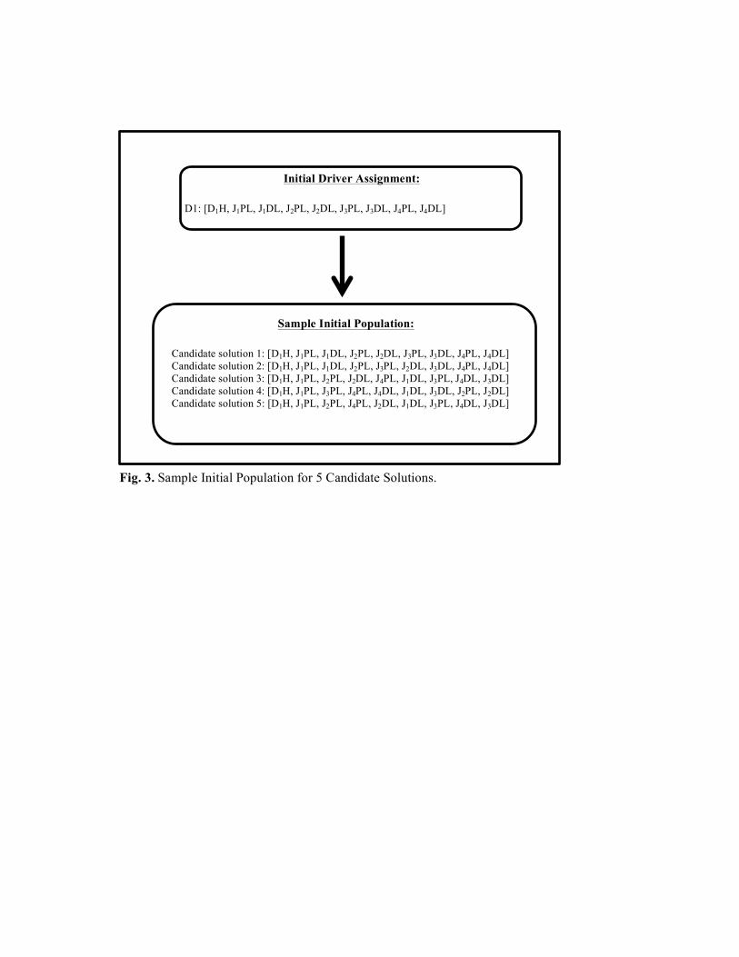
Initial Driver Assignment: D1: [D1H, J1PL, J1DL, J2PL, J2DL, J3PL, J3DL, J4PL, J4DL]

Sample Initial Population: Candidate solution 1: [D1H, J1PL, J1DL, J2PL, J2DL, J3PL, J3DL, J4PL, J4DL] Candidate solution 2: [D1H, J1PL, J1DL, J2PL, J3PL, J2DL, J3DL, J4PL, J4DL] Candidate solution 3: [D1H, J1PL, J2PL, J2DL, J4PL, J1DL, J3PL, J4DL, J3DL] Candidate solution 4: [D1H, J1PL, J3PL, J4PL, J4DL, J1DL, J3DL, J2PL, J2DL] Candidate solution 5: [D1H, J1PL, J2PL, J4PL, J2DL, J1DL, J3PL, J4DL, J3DL]

Fig. 3. Sample Initial Population for 5 Candidate Solutions.

Selected Candidate Solution for Mutation:

[D1H, J1PL, J1DL, J2PL, J3PL, J2DL, J3DL, J4PL, J4DL]

Step 1: Select a gene to mutate. Suppose the gene J1DL was selected.

[D1H, J1PL, J1DL, J2PL, J3PL, J2DL, J3DL, J4PL, J4DL]

Step 2: With a .5 probability, exchange the selected

gene with its neighbor to the right or left. Suppose this probability process selected the left neighbor, J1PL. These two genes are exchanged.

Mutated Candidate Solution: [D1H, J1DL, J1PL , J2PL, J3PL, J2DL, J3DL, J4PL, J4DL]

Step 3: Check the validity of the mutated solution.

This solution is not valid since the ordering has job J1 being dropped off before it was picked up. Therefore we must abandon this solution.

Fig. 4. Sample Mutation Process Yielding an Invalid Solution.

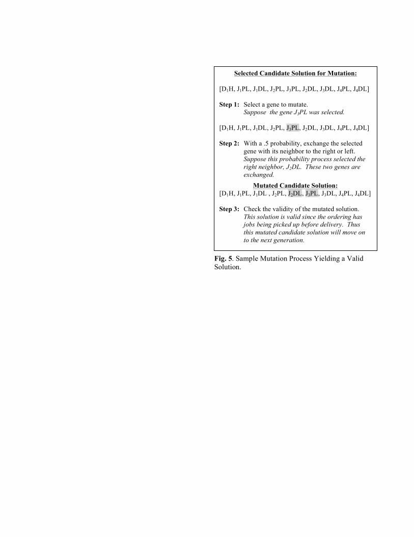
Selected Candidate Solution for Mutation: [D1H, J1PL, J1DL, J2PL, J3PL, J2DL, J3DL, J4PL, J4DL] Step 1: Select a gene to mutate. Suppose the gene J3PL was selected. [D1H, J1PL, J1DL, J2PL, J3PL, J2DL, J3DL, J4PL, J4DL] Step 2: With a .5 probability, exchange the selected

gene with its neighbor to the right or left. Suppose this probability process selected the right neighbor, J2DL. These two genes are exchanged.

Mutated Candidate Solution: [D1H, J1PL, J1DL , J2PL, J2DL, J3PL, J3DL, J4PL, J4DL] Step 3: Check the validity of the mutated solution.

This solution is valid since the ordering has jobs being picked up before delivery. Thus this mutated candidate solution will move on to the next generation.

Fig. 5. Sample Mutation Process Yielding a Valid Solution.

Fig. 6. Graph of GA solutions and Pareto front for our Sample Data Problem

GA solutions

Pareto Front solutions

4

5

6

7

8

9

10

11

12

800 900 1000 1100 1200 1300 1400 1500 1600 1700

#ofDriv

ers

Time(minutes)

Fig. 7. Graph of GA solutions and Pareto front for Day 1 jobs.

GA solutions

Pareto Front solutions

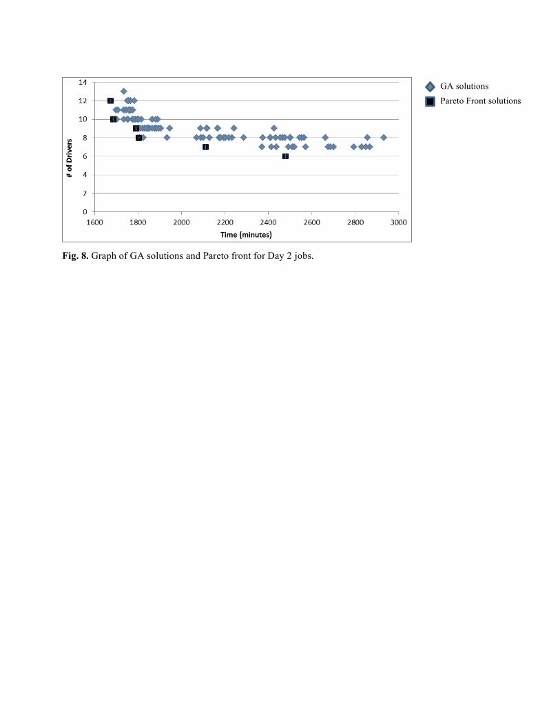
Fig. 8. Graph of GA solutions and Pareto front for Day 2 jobs.

GA solutions

Pareto Front solutions

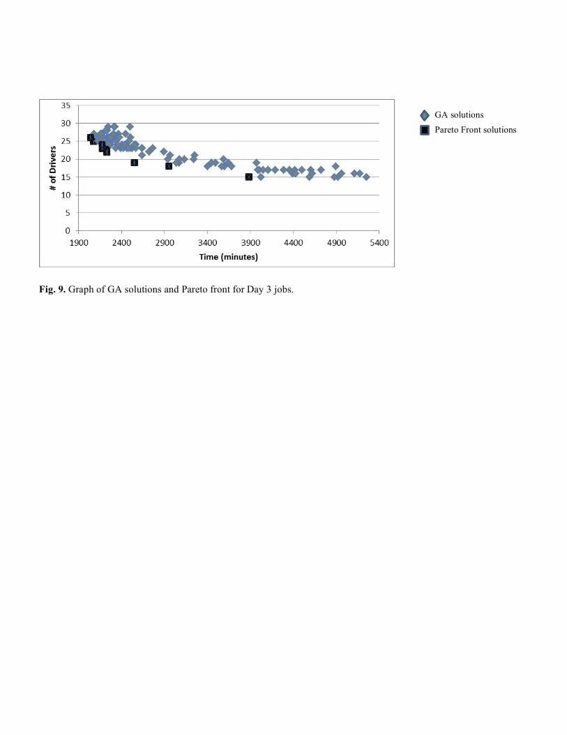
Fig. 9. Graph of GA solutions and Pareto front for Day 3 jobs.

GA solutions

Pareto Front solutions

Table 1 Sample Potential Drivers List

Job Drivers Available to Service Job

Job Weight

J1 D1, D2 300 lbs J2 D1, D2, D3 400 lbs J3 D2, D3 850 lbs J4 D1, D2, D3 400 lbs J5 D4 600 lbs

Table 2 Sample Input Data

Job#

Pickup Tim

e

Delivery T

ime

Pickup Location

Delivery L

ocation

(Max V

ehicle Type C

apacity) V

ehicle Type

Job Weight

J1 6:30 16:00 134 76 C (1,500) 280 J2 9:30 11:30 51 68 S (2,000) 180 J3 8:00 11:00 130 88 T (43,500) 42000 J4 8:30 11:30 127 98 B (10,500) 1000 J5 9:00 11:30 139 124 C (1,500) 300 J6 8:30 11:30 136 65 B (10,500) 468 J7 7:00 9:00 43 42 C (1,500) 500 J8 8:00 10:00 43 121 C (1,500) 25 J9 9:00 11:00 103 55 C (1,500) 200 J10 8:00 9:00 43 141 C (1,500) 1300 J11 8:00 10:30 100 128 B (10,500) 10,000

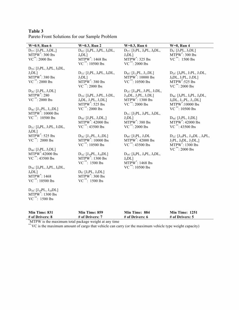
Table 3 Pareto Front Solutions for our Sample Problem

W=0.9, Run 6 W=0.3, Run 2 W=0.3, Run 6 W=0, Run 4 D27: [J5PL, J5DL,] MTPW*: 300 lbs VC**: 2000 lbs D25: [J2PL, J9PL, J9DL, J2DL] MTPW*: 380 lbs VC **: 2000 lbs D26: [J1PL, J1DL] MTPW*: 280 VC **: 2000 lbs D46: [J11PL, J11DL] MTPW*: 10000 lbs VC **: 10500 lbs D31: [J8PL, J7PL, J7DL, J8DL] MTPW*: 525 lbs VC **: 2000 lbs D48: [J3PL, J3DL] MTPW*:42000 lbs VC **: 43500 lbs D38: [J6PL, J4PL, J4DL, J6DL] MTPW*: 1468 VC **: 10500 lbs D18: [J10PL, J10DL] MTPW*: 1300 lbs VC **: 1500 lbs Min Time: 831 # of Drivers: 8

D42: [J6PL, J4PL, J4DL, J6DL] MTPW*: 1468 lbs VC **: 10500 lbs D33: [J2PL, J9PL, J9DL, J2DL] MTPW*: 380 lbs VC **: 2000 lbs D19: [J8PL, J7PL, J7DL, J8DL, J1PL, J1DL] MTPW*: 525 lbs VC **: 2000 lbs D50: [J3PL, J3DL,] MTPW*: 42000 lbs VC **: 43500 lbs D36: [J11PL, J11DL] MTPW*: 10000 lbs VC **: 10500 lbs D16: [J10PL, J10DL] MTPW*: 1300 lbs VC **: 1500 lbs D9: [J5PL, J5DL] MTPW*: 300 lbs VC **: 1500 lbs Min Time: 859 # of Drivers: 7

D27: [J5PL, J8PL, J8DL, J5DL] MTPW*: 325 lbs VC **: 2000 lbs D45: [J11PL, J11DL] MTPW*: 10000 lbs VC **: 10500 lbs D25: [J10PL, J7PL, J7DL, J10DL, J1PL, J1DL] MTPW*: 1300 lbs VC **: 2000 lbs D31: [J2PL, J9PL, J9DL, J2DL] MTPW*: 380 lbs VC **: 2000 lbs D49: [J3PL, J3DL MTPW*: 42000 lbs VC **: 43500 lbs D39: [J6PL, J4PL, J4DL, J6DL] MTPW*: 1468 lbs VC **: 10500 lbs Min Time: 884 # of Drivers: 6

D6: [J5PL, J5DL] MTPW*: 300 lbs VC **: 1500 lbs D25: [J8PL, J7PL, J7DL, J8DL, J1PL, J1DL] MTPW*:525 lbs VC **: 2000 lbs D46: [J6PL, J4PL, J4DL, J6DL, J11PL, J11DL] MTPW*:10000 lbs VC **: 10500 lbs D50: [J3PL, J3DL] MTPW*: 42000 lbs VC **: 43500 lbs D22: [J10PL, J10DL , J9PL, J2PL, J9DL, J2DL,] MTPW*: 1300 lbs VC **: 2000 lbs Min Time: 1251 # of Drivers: 5

*MTPW is the maximum total package weight at any time ** VC is the maximum amount of cargo that vehicle can carry (or the maximum vehicle type weight capacity)

1

Table 4 Details for each Job on Days 1, 2 and 3.

Day 1

Job #

Pickup Tim

e

Delivery T

ime

Pickup L

ocation

Delivery

Location

Vehicle T

ype

J1 6:30 16:00 134 76 C J2 9:30 17:00 137 111 S J3 9:30 11:30 119 78 C J4 11:45 13:45 64 60 C J5 9:30 11:30 51 68 S

J6 8:00 11:00 130 88 T J7 6:30 7:30 82 43 C J8 8:00 10:00 40 104 C J9 8:30 11:30 127 98 B J10 9:00 11:30 139 124 C J11 8:30 11:30 136 65 B J12 7:00 9:00 43 42 C J13 8:00 10:00 43 121 C J14 9:00 11:00 103 55 C J15 8:00 9:00 43 141 S J16 8:00 10:30 100 128 B

Day 2

Job #

Pickup Tim

e

Delivery T

ime

Pickup L

ocation

Delivery

Location

Vehicle T

ype

J1 11:45 13:45 94 60 C J2 8:30 10:30 85 135 S J3 9:00 12:00 46 99 B J4 9:00 12:00 41 99 B J5 10:00 13:00 127 98 B J6 10:00 13:00 96 48 B J7 9:30 11:30 75 132 C J8 8:00 10:00 141 95 C J9 7:00 16:00 69 62 C J10 7:00 9:00 121 43 C J11 7:00 10:00 43 95 C J12 5:00 7:00 43 121 C J13 7:00 9:00 43 109 C J14 9:00 8:30 100 73 B J15 9:00 11:00 100 45 B

Day 3

Job #

Pickup Tim

e

Delivery T

ime

Pickup L

ocation

Delivery

Location

Vehicle T

ype

J1 14:00 16:00 92 81 C J2 8:30 10:30 122 90 C J3 10:30 13:30 56 115 B J4 9:00 11:00 71 72 S J5 15:30 17:30 116 53 C J6 9:00 11:00 110 118 C J7 13:30 16:30 67 82 B J8 9:00 12:00 107 130 B J9 9:00 11:00 84 93 S J10 11:00 13:30 61 114 S J11 7:00 10:00 89 63 B J12 13:00 15:00 91 66 C J13 10:30 12:30 97 50 S J14 13:30 14:30 40 86 C J15 14:30 15:30 86 40 C J16 7:30 9:30 141 43 C J17 9:00 11:00 74 58 C J18 9:00 12:00 74 105 C J19 9:00 11:30 74 140 C J20 9:00 11:30 74 133 C J21 9:00 11:00 74 87 C J22 9:00 11:00 121 95 C J23 9:00 12:00 74 83 C

Table 5 Summary of Pareto Front Results for our 3 Problems

W Day 1: 16 Jobs Day 2: 15 Jobs Day 3: 39 Jobs (f1

*= 1260, f2*= 8) (f1

*= 1673, f2*= 6) (f1

*= 2039, f2*= 15)

1 - 1673 minutes, 12 drivers 2073 minutes, 25 drivers - - 2039 minutes, 26 drivers 0.9 1310 minutes, 11 drivers - - 1243 minutes, 13 drivers - - 0.8 1281 minutes, 12 drivers 1686 minutes, 10 drivers 2177 minutes, 23 drivers 0.7 - 1804 minutes, 8 drivers - - 1791 minutes, 9 drivers - 0.6 - - 2228 minutes, 22 drivers - - 2174 minutes, 24 drivers 0.5 1414 minutes, 9 drivers - - 0.4 - - - 0.3 1352 minutes, 10 drivers 2111 minutes, 7 drivers 2952 minutes, 18 drivers 0.2 2533 minutes, 7 drivers - 2548 minutes, 19 drivers 0.1 1785 minutes, 8 drivers - 3883 minutes, 15 drivers 0 - 2479 minutes, 6 drivers -

Table 6 Pareto Front Solutions from our GA and the BSL Job Allocations for the Day 1 Jobs.

W=0.9, Run 1 W=0.9, Run 9 W=0.8, Run 5 W=0.5, Run 2 D30: [J3PL, J3DL, J5PL, J5DL] D32: [J1PL, J1DL] D35: [J16PL, J16DL] D62: [J6PL, J6DL] D22: [J10PL, J13PL, J13DL, J10DL] D3: [J14PL, J8PL, J8DL, J14DL] D25: [J15PL, J12PL, J12DL, J15DL] D17: [J4PL, J4DL] D14: [J7PL, J7DL] D28: [J2PL, J2DL] D47: [J11PL, J9PL, J9DL, J11DL] Min Time: 1310 # of Drivers: 11

D21: [ J4PL, J4DL] D27: [J10PL, J10DL] D31: [ J12PL, J7PL, J7DL, J12DL] D32: [J2PL, J2DL] D35: [J11PL, J9PL, J9DL, J11DL] D33: [J5PL, J5DL] D62: [J6PL, J6DL] D4: [J15PL, J15DL] D3: [J3PL, J3DL] D42: [J16PL, J16DL] D9: [J13PL, J13DL, J1PL, J1DL] D16: [ J14PL, J14DL] D13: [J8PL, J8DL] Min Time: 1243 # of Drivers:13

D30: [J15PL, J12PL, J12DL, J15DL] D61: [J6PL, J6DL] D44: [J11PL, J9PL, J9DL, J11DL] D35: [J16PL, J16DL] D32: [J1PL, J1DL] D33: [J7PL, J7DL] D1: [J3PL, J3DL] D22: [J8PL, J8DL, J2PL, J2DL] D23: [J5PL, J14PL, J14DL, J5DL] D18: [J4PL, J4DL] D7: [J13PL, J13DL] D27: [J10PL, J10DL] Min Time: 1281 # of Drivers: 12

D46: [J11PL, J9PL, J9DL, J11DL] D50: [J6PL, J6DL] D19: [J15PL, J12PL, J12DL, J15DL, J2PL, J2DL] D34: [J3PL, J14PL, J5PL, J3DL, J14DL, J5DL] D25: [J8PL, J8DL, J1PL, J1DL] D43: [J16PL, J16DL] D15: [J10PL, J13PL, J13DL, J10DL] D14: [J4PL, J4DL] D13: [J7PL, J7DL] Min Time: 1414 # of Drivers: 9

W=0.3, Run 8 W=0.2, Run 9 W=0.1, Run 9 BSL Job Assignments D31: [J5PL, J3PL, J3DL, J5DL] D20: [J14PL, J14DL, J13PL, J13DL, J10PL, J10DL] D37: [J11PL, J9PL, J9DL, J11DL] D4: [J4PL, J4DL] D34: [J8PL, J8DL, J2PL, J2DL] D6: [J12PL, J12DL, J1PL, J1DL] D77: [J6PL, J6DL] D25: [J7PL, J7DL] D28: [ J15PL, J15DL] D47: [ J16PL, J16DL] Min Time: 1352 # of Drivers: 10

D30: [J5PL, J15PL, J13PL, J4PL, J15DL, J5DL, J4DL, J13DL, J2PL, J2DL] D45: [J11PL, J9PL, J9DL, J11DL] D62: [J6PL, J6DL] D19: [ J10PL, J10DL] D34: [J8PL, J8DL, J12PL, J12DL, J14PL, J14DL] D21: [J3PL, J7PL, J7DL, J3DL, J1PL, J1DL] D38: [J16PL, J16DL] Min Time: 2533 # of Drivers: 7

D30: [J7PL, J7DL] D35: [J11PL, J9PL, J9DL, J11DL] D1: [J3PL, J4PL, J3DL, J4DL] D4: [J13PL, J12PL, J12DL, J13DL, J1PL, J14PL, J14DL, J1DL] D57: [J6PL, J6DL] D3: [ J15PL, J15DL, J8PL, J8DL] D41: [J16PL, J16DL] D29: [J10PL, J10DL, J5PL, J5DL, J2PL, J2DL] Min Time: 1785 # of Drivers: 8

D2:[ J13] D3 :[ J10] D7: [J1] D19: [J8] D20: [J7, J12, J15] D22:[J3] D31: [J5] D41: [J2] D44: [J9] D45: [J11] D57: [J4] D63: [J16] D70: [J6] D77: [J14] Min Time: 1571 # of Drivers: 14

Table 7 Pareto Front Solutions from our GA and the BSL Job Allocations for the Day 2 Jobs.

W=1, Run 8 W=0.8, Run 2 W=0.7, Run 5 W=0.7, Run 8 D45: [J3PL, J4PL, J3DL, J4DL] D34: [J2PL, J2DL] D39: [J5PL, J5DL] D23: [J1PL, J1DL] D38: [J15PL, J14PL, J14DL, J15DL] D5: [J13PL, J13DL] D25: [J9PL, J11PL, J9DL, J11DL] D7: [J12PL, J12DL] D17: [J8PL, J8DL] D42: [J6PL, J6DL] D29: [J7PL, J7DL] D12: [J10PL, J10DL] Min Time: 1673 # of Drivers: 12

D27: [J2PL, J2DL] D45: [J6PL, J6DL] D25: [J12PL, J12DL] D42: [J15PL, J14PL, J14DL, J15DL] D46: [J5PL, J5DL] D26: [J7PL, J8PL, J8DL, J7DL] D12: [J10PL, J13PL, J10DL, J13DL] D15: [J1PL, J1DL] D18: [J9PL, J11PL, J9DL, J11DL] D47: [J3PL, J4PL, J3DL, J4DL] Min Time: 1686 # of Drivers: 10

D4: [J8PL, J8DL] D43: [J6PL, J6DL, J3PL, J5PL, J3DL, J5DL] D33: [J12PL, J12DL] D30: [J2PL, J2DL] D31: [J7PL, J9PL, J7DL, J9DL] D12: [J10PL, J10DL, J11PL, J13PL, J13DL, J11DL] D37: [ J4PL, J4DL, J14PL, J15PL, J14DL, J15DL] D22: [J1PL, J1DL] Min Time: 1804 # of Drivers: 8

D27: [J2PL, J2DL] D40: [J6PL, J6DL] D3: [J1PL, J1DL] D28: [J12PL, J12DL] D15: [J10PL, J9PL, J10DL, J11PL, J9DL, J11DL] D36: [J3PL, J4PL, J3DL, J4DL] D17: [J7PL, J7DL] D38: [J5PL, J5DL, J15PL, J14PL, J14DL, J15DL] D7: [J13PL, J13DL, J8PL, J8DL] Min Time: 1791 # of Drivers: 9

W=0.3, Run 7 W=0, Run 6 BSL Job

Assignments D30: [J7PL, J7DL] D2: [J1PL, J1DL] D34: [J11PL, J12PL, J12DL, J10PL, J10DL, J8PL, J8DL, J11DL, J2PL, J2DL] D37: [J4PL, J4DL, J5PL, J5DL] D36: [J3PL, J3DL] D38: [J6PL, J6DL, J15PL, J14PL, J14DL, J15DL] D7: [J13PL, J9PL, J13DL, J9DL] Min Time: 2111 # of Drivers: 7

D45: [J5PL, J5DL, J14PL, J15PL, J14DL, J15DL] D44: [J6PL, J6DL, J3PL, J3DL] D39: [J4PL, J4DL] D26: [J2PL, J2DL, J8PL, J8DL, J9PL, J9DL, J1PL, J1DL] D18: [J11PL, J11DL, J7PL, J7DL] D27: [J10PL, J12PL, J13PL, J10DL, J12DL, J13DL] Min Time: 2479 # of Drivers: 6

D2:[ J13] D4:[ J1] D8: [J7] D9: [J10] D19: [J8, J11] D20:[J12] D22: [J2] D23: [J9] D35: [J5, J14, J15] D36: [J6] D40: [J3] D41: [J4] Min Time: 1858 # of Drivers: 12

Table 8 Pareto Front Solutions from our GA and the BSL Job Allocations for the Day 3 Jobs.

W=1, Run 1 W=1, Run 6 W=.8, Run 5 W=.6, Run 5 D44: [J11PL, J11DL] D27: [J13PL, J13DL] D41: [J7PL, J7DL] D25: [J23PL, J37PL, J23DL, J37DL] D26: [J38PL, J38DL] D19: [J34PL, J22PL, J34DL, J9PL, J9DL, J22DL]D20: [J10PL, J10DL] D35: [J8PL, J8DL] D21: [J16PL, J16DL] D39: [J3PL, J3DL] D28: [J4PL, J4DL, J32PL, J32DL] D5: [J30PL, J36PL, J30DL, J36DL] D3: [J18PL, J18DL] D32: [J14PL, J14DL] D33: [J17PL, J20PL, J20DL, J17DL] D30: [J27PL, J31PL, J29PL, J2PL, J27DL, J31DL, J29DL, J2DL] D31: [J25PL, J35PL, J25DL, J35DL] D12: [J6PL, J6DL] D13: [J24PL, J24DL] D14: [J33PL, J21PL, J21DL, J33DL] D15: [J28PL, J19PL, J28DL, J19DL] D16: [J5PL, J5DL] D17: [J12PL, J12DL] D18: [J15PL, J1PL, J15DL, J1DL]] D7: [J39PL, J39DL, J26PL, J26DL] Min Time: 2073 # of Drivers: 25

D46: [J11PL, J11DL] D10: [J1PL, J1DL] D27: [J13PL, J13DL] D25: [J10PL, J10DL] D43: [J7PL, J7DL] D19: [J2PL, J2DL] D20: [J19PL, J23PL, J20PL, J20DL, J19DL, J23DL] D36: [J3PL, J3DL] D22: [J5PL, J5DL] D39: [J8PL, J8DL] D29: [J24PL, J24DL] D28: [J9PL, J25PL, J4PL, J4DL, J39PL, J39DL, J25DL, J9DL] D6: [J34PL, J34DL] D5: [J12PL, J12DL] D34: [J15PL, J15DL] D3: [J22PL, J35PL, J33PL, J33DL, J35DL, J22DL] D32: [J36PL, J29PL, J21PL, J29DL, J21DL, J36DL] D1: [J38PL, J38DL] D31: [J37PL, J37DL] D12: [J14PL, J14DL] D13: [J18PL, J18DL] D14: [J6PL, J6DL] D15: [J30PL, J26PL, J26DL, J30DL] D16: [J17PL, J31PL, J32PL, J27PL, J27DL, J31DL, J32DL, J17DL] D9: [J16PL, J16DL] D7: [J28PL, J28DL] Min Time: 2039 # of Drivers: 26

D40: [J8PL, J8DL] D41: [J3PL, J3DL] D25: [J5PL, J5DL] D26: [J14PL, J14DL] D19: [J21PL, J9PL, J21DL, J9DL] D20: [J25PL, J28PL, J25DL, J28DL, J10PL, J10DL] D35: [J7PL, J7DL] D23: [J12PL, J12DL] D37: [J11PL, J11DL] D22: [J37PL, J32PL, J33PL, J32DL, J33DL, J37DL] D29: [J27PL, J26PL, J27DL, J26DL] D28: [J4PL, J4DL, J30PL, J30DL] D6: [J29PL, J29DL] D5: [J15PL, J15DL] D34: [J39PL, J39DL, J36PL, J36DL] D3: [J24PL, J17PL, J23PL, J18PL, J24DL, J23DL, J18DL, J17DL]D32: [J22PL, J35PL, J35DL, J22DL] D30: [J13PL, J13DL] D13: [J20PL, J20DL] D16: [J19PL, J19DL] D9: [J38PL, J38DL, J16PL, J16DL, J2PL, J2DL] D8: [J31PL, J34PL, J6PL, J6DL, J34DL, J31DL] D18: [J1PL, J1DL] Min Time: 2177 # of Drivers: 23

D20: [J6PL, J32PL, J2PL, J2DL, J32DL, J6DL, J10PL, J10DL]D19: [J28PL, J28DL] D24: [J9PL, J22PL, J25PL, J25DL, J9DL, J22DL]D23: [J15PL, J15DL] D27: [J13PL, J13DL] D30: [J1PL, J14PL, J14DL, J1DL] D31: [J4PL, J4DL, J23PL, J23DL] D1: [J37PL, J36PL, J29PL, J34PL, J34DL, J29DL, J36DL, J37DL] D33: [J17PL, J17DL] D37: [J8PL, J8DL] D3: [J12PL, J12DL] D36: [J3PL, J3DL] D6: [J16PL, J5PL, J5DL, J16DL] D5: [J33PL, J35PL, J21PL, J30PL, J30DL, J33DL, J35DL, J21DL]D8: [J39PL, J39DL] D40: [J11PL, J11DL] D17: [J38PL, J38DL] D43: [J7PL, J7DL] D9: [J20PL, J20DL] D14: [J27PL, J18PL, J27DL, J18DL] D13: [J31PL, J26PL, J26DL, J31DL] D12: [J24PL, J19PL, J24DL, J19DL] Min Time: 2228 # of Drivers: 22

Table 8 (Continued) W=.6, Run 10 W=.3, Run 4 W=.2, Run 6 W=0, Run 6 D20: [J10PL, J10DL] D19: [J20PL, J20DL] D21: [J37PL, J21PL, J26PL, J26DL, J21DL, J37DL] D23: [J13PL, J13DL] D26: [J30PL, J33PL, J30DL, J33DL] D25: [J15PL, J1PL, J15DL, J1DL] D27: [J22PL, J4PL, J4DL, J22DL] D30: [J12PL, J12DL] D32: [J9PL, J29PL, J29DL, J9DL] D34: [J27PL, J35PL, J2PL, J27DL, J35DL, J2DL] D4: [J24PL, J36PL, J24DL, J36DL] D3: [J32PL, J32DL] D5: [J19PL, J6PL, J6DL, J19DL] D7: [J28PL, J28DL] D9: [J31PL, J31DL] D36: [J8PL, J8DL] D39: [J11PL, J11DL] D18: [J17PL, J23PL, J34PL, J17DL, J34DL, J39PL, J39DL, J23DL] D40: [J7PL, J7DL] D16: [J18PL, J25PL, J25DL, J18DL] D15: [J5PL, J5DL] D14: [J38PL, J38DL, J16PL, J16DL] D13: [J14PL, J14DL] D47: [J3PL, J3DL] Min Time: 2174 # of Drivers: 24

D11: [J18PL, J26PL, J17PL, J26DL, J17DL, J18DL] D10: [J38PL, J38DL] D19: [J16PL, J16DL] D24: [J20PL, J19PL, J28PL, J28DL, J20DL, J19DL] D26: [J9PL, J24PL, J25PL, J23PL, J25DL, J9DL, J24DL, J23DL] D25: [J15PL, J1PL, J15DL, J1DL] D27: [J22PL, J13PL, J13DL, J22DL, J14PL, J14DL] D30: [J4PL, J4DL, J21PL, J33PL, J5PL, J33DL, J21DL, J5DL] D31: [J30PL, J30DL, J36PL, J36DL, J10PL, J10DL] D32: [J35PL, J34PL, J35DL, J34DL] D35: [J7PL, J7DL] D3: [J6PL, J31PL, J29PL, J37PL, J29DL, J6DL, J31DL, J37DL] D36: [J8PL, J8DL] D5: [J39PL, J39DL] D43: [J11PL, J3PL, J11DL, J3DL] D17: [J12PL, J12DL] D16: [J2PL, J2DL] D9: [J27PL, J32PL, J27DL, J32DL] Min Time: 2952 # of Drivers: 18

D22: [J25PL, J37PL, J25DL, J31PL, J39PL, J39DL, J31DL, J37DL, J5PL, J5DL] D24: [J20PL, J20DL] D23: [J35PL, J9PL, J35DL, J9DL] D26: [J29PL, J18PL, J29DL, J19PL, J19DL, J18DL, J10PL, J10DL, J14PL, J14DL] D25: [J1PL, J1DL] D29: [J4PL, J4DL] D30: [J12PL, J12DL] D31: [J13PL, J13DL] D33: [J17PL, J30PL, J26PL, J26DL, J30DL, J17DL] D37: [J3PL, J3DL, J8PL, J8DL] D34: [J23PL, J23DL] D36: [J7PL, J7DL] D7: [J33PL, J21PL, J34PL, J34DL, J21DL, J33DL] D18: [J27PL, J27DL] D43: [J11PL, J11DL] D9: [J15PL, J15DL] D15: [J36PL, J6PL, J22PL, J6DL, J22DL, J36DL] D13: [J38PL, J38DL, J16PL, J16DL, J2PL, J2DL] D12: [J28PL, J32PL, J24PL, J24DL, J28DL, J32DL] Min Time:2548 # of Drivers: 19

D11: [J26PL, J34PL, J1PL, J34DL, J26DL, J1DL] D21: [J9PL, J9DL, J20PL, J20DL] D24: [J12PL, J12DL] D23: [J33PL, J4PL, J16PL, J33DL, J16DL, J4DL] D27: [J31PL, J31DL] D30: [J27PL, J17PL, J23PL, J27DL, J17DL, J23DL, J10PL, J10DL] D31: [J6PL, J18PL, J6DL, J18DL, J13PL, J14PL, J14DL, J13DL] D2: [J36PL, J37PL, J22PL, J22DL, J37DL, J36DL] D1: [J25PL, J28PL, J32PL, J28DL, J15PL, J15DL, J25DL, J32DL] D33: [J29PL, J35PL, J38PL, J38DL, J2PL, J29DL, J2DL, J35DL] D36: [J7PL, J7DL] D38: [J11PL, J11DL] D41: [J3PL, J3DL, J8PL, J8DL] D17: [J30PL, J19PL, J24PL, J30DL, J24DL, J19DL] D12: [J21PL, J5PL, J5DL, J39PL, J39DL, J21DL] Min Time: 3883 # of Drivers: 15

BSL Job Assignments D1: [J21, J29] D9: [J17] D20:[ J2, J22, J25, J38] D21: [J5] D22: [J4, J16, J18, J23, J24, J28] D23:[ J1] D24: [J12, J39] D25: [J13] D26: [J19 , J20] D27: [J14, J15] D31:[J6, J34, J35] D33: [J9, J10] D34: [J26, J27, J30, J31, J32, J33, J36, J37] D37: [J3, J11] D40: [J7, J8] Min Time: 3698 # of Drivers: 15