Final Report

A bioinformatic approach to inter functional interactions within protein sequences

AFOSR/AOARD Reference Number: USAFAOGA07: FA4869-07-1-4050

AFOSR/AOARD Program Manager: Hiroshi Motoda, Ph.D.

Period of Performance: January 1, 2008 to December 31, 2008

Submission Date: 23 Feb 2009

PI: Professors GI Webb and J Whisstock

Report Documentation Page Form ApprovedOMB No. 0704-0188

Public reporting burden for the collection of information is estimated to average 1 hour per response, including the time for reviewing instructions, searching existing data sources, gathering andmaintaining the data needed, and completing and reviewing the collection of information. Send comments regarding this burden estimate or any other aspect of this collection of information,including suggestions for reducing this burden, to Washington Headquarters Services, Directorate for Information Operations and Reports, 1215 Jefferson Davis Highway, Suite 1204, ArlingtonVA 22202-4302. Respondents should be aware that notwithstanding any other provision of law, no person shall be subject to a penalty for failing to comply with a collection of information if itdoes not display a currently valid OMB control number.

1. REPORT DATE 26 FEB 2009

2. REPORT TYPE FInal

3. DATES COVERED 01-08-2007 to 01-08-2008

4. TITLE AND SUBTITLE A bioinformatic approach to infer functional interactions within protein sequences

5a. CONTRACT NUMBER FA48690714050

5b. GRANT NUMBER

5c. PROGRAM ELEMENT NUMBER

6. AUTHOR(S) Geof Webb

5d. PROJECT NUMBER

5e. TASK NUMBER

5f. WORK UNIT NUMBER

7. PERFORMING ORGANIZATION NAME(S) AND ADDRESS(ES) Faculty of Information Technology, Monash University,Building 63,Wellington Road,Clayton 3800,Australia,au,3800

8. PERFORMING ORGANIZATIONREPORT NUMBER N/A

9. SPONSORING/MONITORING AGENCY NAME(S) AND ADDRESS(ES) AOARD, UNIT 45002, APO, AP, 96337-5002

10. SPONSOR/MONITOR’S ACRONYM(S) AOARD

11. SPONSOR/MONITOR’S REPORT NUMBER(S) AOARD-074050

12. DISTRIBUTION/AVAILABILITY STATEMENT Approved for public release; distribution unlimited

13. SUPPLEMENTARY NOTES

14. ABSTRACT The primary purpose of the current project was to evaluate the techniques they had developed to inferfunctional interactions between the sites within a protein and, if appropriate, refine them in the light of theresults of evaluation. The initial results revealed significant limitations of their preliminary approaches. Asa result of this project, it is now apparent that deep understanding of the significance of co-evolutionbetween sites within a protein family requires sophisticated methods for identifying large groups ofco-evolving sites, in some cases more than 100 sites that all co-evolve with one another. They havedeveloped techniques that first identify all pairs of co-evolved sites and then identify all maximal cliquesthat can be formed from these pairs. In the process they developed a new data mining technique,association networks. In a separate study they have applied their approaches to the problem of wholegenome alignment. They have successfully developed an engine that can align whole genomes and areextending it to handle the case of sequence reordering.

15. SUBJECT TERMS Computer Science, Information Technology, Data Mining, Biology

16. SECURITY CLASSIFICATION OF: 17. LIMITATION OF ABSTRACT Same as

Report (SAR)

18. NUMBEROF PAGES

49

19a. NAME OFRESPONSIBLE PERSON

a. REPORT unclassified

b. ABSTRACT unclassified

c. THIS PAGE unclassified

Objectives: Briefly summarize the objectives of the research effort or the statement of work. The objectives of this research were to assess experimentally our preliminary techniques for identifying co-evolution of functional sites within protein families and to refine the techniques in the light of the outcomes of that evaluation. Status of effort: Experimental evaluation revealed significant failings in our proposed approach to identifying co-evolution of functional sites within protein families. With further research, we developed new techniques that overcome this problem and for which preliminary results are encouraging. We are in the process of developing a web server for these revised techniques (http://versi-3.its.monash.edu.au:8080/GDM/index.jsp) and of finalizing the research into their relative efficacy. We are also developing techniques for aligning whole genomes. A web server is also being developed for these techniques (http://vbc.med.monash.edu.au/~kmahmood/EGA/) and a paper will be submitted to the Journal of Molecular Biology. Abstract: Briefly describe research accomplishments, their significance to the field, and their relationship to the

original goals. This project investigated novel computational techniques to infer functional interactions between the sites within a protein. At the start of this project we had developed computational techniques with theoretical capacity to infer functional interactions between the sites with a protein. The primary purpose of the current project was to evaluate those techniques and, if appropriate, refine them in the light of the results of evaluation. Our initial results revealed significant limitations of our preliminary approaches. As a result of this project, it is now apparent that deep understanding of the significance of co-evolution between sites within a protein family requires sophisticated methods for identifying large groups of co-evolving sites, in some cases more than 100 sites that all co-evolve with one another. We have now developed techniques that first identify all pairs of co-evolved sites and then identify all maximal cliques that can be formed from these pairs. In the process we developed a new data mining technique, association networks (paper submitted to the ACM SIGKDD Conference on Knowledge Discovery and Data Mining.) In a separate study we have applied our approaches to the problem of whole genome alignment. We have successfully developed an engine that can align whole genomes and are extending it to handle the case of sequence reordering. Personnel Supported: List the professional personnel supported by the contract and/or the personnel who

participated significantly in the research effort. Prof Geoffrey Webb Prof James Whisstock Dr Jianging Song Mr Khalid Mahmood Mr Cyril Reboul Ms Wan Ting Kan Publications: List peer-reviewed publications submitted and/or accepted during the contract period. A computational pipeline for Encapsulated Gene-by-gene Alignment (EGA) of whole proteome sequences. Khalid Mahmood, Noel G. Faux, Arun S. Konagurthu, Ashley M. Buckle, Geoffrey I. Webb and James C. Whisstock. To be submitted to the Journal of Molecular Biology. Preliminary draft attached.

Identification and analysis of co-evolving positions in diverse protein families. Khalid Mahmood, Jianging Song, Cyril Reboul, Wan Ting Kan, Geoffrey I. Webb and James C. Whisstock. To be submitted to BMC Bioinformatics. Outline attached. Association networks: A new approach to association analysis Geoffrey I. Webb, Khalid Mahmood and Jianging Song, Submitted to the 2009 ACM SIGKDD Conference on Knowledge Discovery and Data Mining Attached.

Interactions: Please list:

(a) Participation/presentations at meetings, conferences, seminars, etc.

Poster presentation: Mahmood K, Faux NG, Konagurthu AS, Buckle AM, Webb GI, Whisstock JC: Encapsulated Gene-by-gene Alignment (EGA) - A new approach to rapidly align whole proteome sequences. In: BacPath9. Lorne, VIC, Australia; 2007. (b) Describe cases where knowledge resulting from your effort is used, or will be used, in a technology application. Not all research projects will have such cases, but please list any that have occurred. Inventions None Honors/Awards: Professor Whisstock was awarded a Federation Fellowship, a prestigious Australian award for eminent researchers. Professor Whisstock was also awarded the 2008 Australian Commonwealth Health Minister's Award for Excellence in Health and Medical Research. Archival Documentation: This section should include a description of your work at a level of technical detail that

you think to be appropriate. Submission of reprints/preprints often satisfies this requirement. If you have questions on how to prepare this section, please discuss this matter with your AOARD program manager.

Software and/or Hardware (if they are specified in the contract as part of final deliverables): Include source

code, brief installation and user guides. Main body of the final report (can be a paper published/to be published) or a draft of the paper) We attach a submitted paper, a draft and an outline.

A computational pipeline for Encapsulated Gene-by-gene Alignment (EGA) of whole proteome sequences

Khalid Mahmood1,2

, Noel G. Faux3, Arun S. Konagurthu

4, Ashley M. Buckle

1,

Geoffrey I. Webb*5 and James C. Whisstock*

1,2

1Department of Biochemistry and Molecular Biology, Monash University, Victoria 3800,

Australia

2ARC Centre of Excellence in Structural and Functional Microbial Genomics, Monash

University, Victoria 3800, Australia

3National ICT Australia Ltd. Victoria Laboratory, Life Sciences Program, The University

of Melbourne, Victoria 3010, Australia

4The Huck Institute of Life Sciences, The Institute for Genomics, Proteomics and

Bioinformatics, Pennsylvania State University, University Park, PA 16802, U.S.A.

5Clayton School of Information Technology, Monash University, Victoria 3800,

Australia

*Corresponding author

Email addresses:

JCW: james.whisstock@med.monash.edu.au

GIW: geoff.webb@infotech.monash.edu.au

Abstract

Background

Comparative proteomics can augment understanding of protein function, the relationship

between organisms, and certain evolutionary processes, through comparison of the

proteomes of different organisms. When protein sequences are ordered according to the

underlying encoding chromosomal DNA, functional correspondence can be inferred for

regions of correspondence between two or more proteomes. The ability to align

proteomes gene product by gene product is thus a crucial tool in comparative proteomics.

Currently, proteome alignments are mainly performed manually using information from

an ensemble of tools. However, as more and more genomic data becomes available it is

desirable that such comparisons are performed robustly, rapidly and automatically.

Results

We have developed Encapsulated Gene-by-gene Alignment (EGA), a computational

pipeline that addresses the problem of whole proteome comparisons. EGA uses protein

similarity and clustering to reduce the input size of the problem and allows dynamic

programming based global comparison of genomes. To the best of our knowledge, EGA

is the first fully automated method to perform such an alignment. Experiments have

shown that EGA delivers a global comparative map and produces reliable and readily

interpretable visualization of the alignments. EGA tool is available as i) a standalone Java

application and ii) a web server that can align various microbial genomes

(http://vbc.med.monash.edu.au/~kmahmood/EGA).

Conclusions

EGA provides a rapid, automated and convenient method that facilitates the detection of

conserved gene strings and provides a global comparative map between a proteome pair.

EGA output provides details about the conserved gene strings and provides a full view of

their context. Analysis of these protein sequence strings may advance understanding of

gene function as well as proteome relationships.

Background Understanding gene order, gene context and conservation in gene clusters in completely

sequenced genomes is a challenging task in comparative genomics. The ever-increasing

availability of whole genome sequences gives the potential to study how genomes are

related in terms of their proteome sequences as well as to investigate how genes function

and whole genomes evolve as the complexity of an organism increases. Global genomic

properties such as similarity in gene content, protein family conservation, and gene order

and context conservation are frequently used in studies to help understand relationships

between organisms [1, 2]. Previous studies have shown that gene order and gene clusters

are well-preserved in closely related genomes [3]. However, identification of such

relationships becomes more challenging as the phylogenetic distance between two

genomes increases. This loss of conservation can mainly be ascribed to operon

disruptions, gene or operon deletions and large-scale genomic rearrangements [4, 5].

However, substantial conservation in gene strings and gene order can be identified at

medium to large phylogenetic distances, as disruptions are moderated by the need to

conserve function [6, 7], as has been observed for proteins that make up the ribosomal

machinery [8].

In the majority of genomes, putative functional annotations can only be made for

~60% of genes. A popular and straightforward approach is to utilize tools such as PSI-

BLAST [9, 10] to identify putative homologues with experimentally verified functions

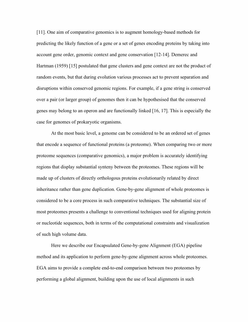
[11]. One aim of comparative genomics is to augment homology-based methods for

predicting the likely function of a gene or a set of genes encoding proteins by taking into

account gene order, genomic context and gene conservation [12-14]. Demerec and

Hartman (1959) [15] postulated that gene clusters and gene context are not the product of

random events, but that during evolution various processes act to prevent separation and

disruptions within conserved genomic regions. For example, if a gene string is conserved

over a pair (or larger group) of genomes then it can be hypothesised that the conserved

genes may belong to an operon and are functionally linked [16, 17]. This is especially the

case for genomes of prokaryotic organisms.

At the most basic level, a genome can be considered to be an ordered set of genes

that encode a sequence of functional proteins (a proteome). When comparing two or more

proteome sequences (comparative genomics), a major problem is accurately identifying

regions that display substantial synteny between the proteomes. These regions will be

made up of clusters of directly orthologous proteins evolutionarily related by direct

inheritance rather than gene duplication. Gene-by-gene alignment of whole proteomes is

considered to be a core process in such comparative techniques. The substantial size of

most proteomes presents a challenge to conventional techniques used for aligning protein

or nucleotide sequences, both in terms of the computational constraints and visualization

of such high volume data.

Here we describe our Encapsulated Gene-by-gene Alignment (EGA) pipeline

method and its application to perform gene-by-gene alignment across whole proteomes.

EGA aims to provide a complete end-to-end comparison between two proteomes by

performing a global alignment, building upon the use of local alignments in such

comparisons. While local alignments can align highly similar smaller segments, it is often

possible to miss weakly conserved segments. Further, since local alignments have no

assumption of orientation, it is difficult to assess their significance, which increases the

chances of detecting false positive alignments. Global alignments, on the other hand, are

based on the assumption that highly conserved and similar segments between a pair of

proteomes maintain similar order and orientation, especially in the cases of related

organisms, or in the case of more distant organisms the conserved segments are relatively

short. EGA is a fully automated approach that given a pair of proteome sequences

provides a dynamic programming-based global gene-by-gene pairwise alignment. This

alignment can then be used to identify proteomic features including putative functional

conservation across a proteome pair.

Methods The EGA pipeline is summarised in Figure 1. Details of steps are described below.

EGA pipeline

Let 1G and

2G denote two whole proteome sequence sets containing m and n protein

sequences respectively. Note that the order in which the protein sequences occur in the

proteome is identical to the order in the genome, and the same definition of gene order is

used for both genomes. Let ),( ji ppS be a measure of similarity between the two protein

sequences, reported as an e-value by BLAST. We denote ! to be the user-defined critical

value of S such that two proteins are similar only if !"),( ji ppS .

Step 1. Finding homologous proteins

Pairwise protein sequence alignment is a common method for finding proteins that may

share similar function and most likely share a common structure. The aim of this step is

to identify proteins within, and across the two proteomes, that exhibit significant

sequence similarity, irrespective of whether they occur in the same organism or within

proximity to one another.

To this end, the proteomes 1G and

2G are concatenated to produce a super-set of

sequences21GG + . This is followed by an all-against-all BLAST search of the

concatenated sequence set. The resulting pairwise local alignments between all inter-

genome protein pairs are recorded along with a similarity score, and a probability score

indicating the chances of the alignment occurring by chance (BLAST reports this as the

e-value). In this step a relatively high cut-off on the e-value (for example 0.001~1.0) is

used to gather the maximum number of possible associations between protein pairs for

input to the next steps in the pipeline.

Step 2. Forming Putative HOmology Groups (PHOGs)

The next task is to cluster similar protein sequences into putative homology groups

(PHOGs). The aim of clustering is three-fold, 1) to classify natural groups of homologous

proteins, 2) to reduce the data dimension and 3) to form an abstract representation of the

common patterns in a cluster. This is performed using the single linkage clustering

strategy. Single linkage clustering is commonly used for grouping biological sequences

because of its simple nature and due to its ability to detect remote relationships through

transitivity [18, 19].

Single linkage clustering starts by placing each protein in its own cluster C i.e.

every cluster contains a single protein sequence. In EGA, the creation of separate PHOGs

is enforced by applying a usually more stringent cluster! on the significance of similarity

such that clusterji ppS !"),( and a minimum sequence identity threshold for the local

alignment identified by Blast. The PHOGs are formed by recursively grouping most

similar proteins based on the chosen thresholds to form iC , until no similar pair is found.

A small cluster! value will result in a large number of single member clusters and

conversely a lenient threshold will result in large loosely cohesive clusters. Therefore a

loose definition of similarity is not sufficient for clustering protein sequences and this is

further compounded by the presence of multiple domains in proteins.

One further constraint that is imposed on cluster linkages is a minimum

participation threshold ! , which reflects the ratio of the local alignment length, as

reported by BLAST, to the total length of the two sequences. This is necessary as the

measures of similarity detailed above are based solely on the alignable region between

two sequences, irrespective of the position of extent of the alignment. For multidomain

proteins, this may result in misleading, transitive linkages and result in the formation of

large superclusters (see additional file 1). A high ! in combination with a low cluster!

value results in the formation of highly cohesive PHOGs. If the genomes being compared

are distant and the thresholds are strong, the result will be a high number of PHOGs the

majority of which contain a single member protein. However in the case of

phylogenetically close genomes, the result will be fewer more cohesive PHOGs, as there

is a higher chance of finding orthologues. As there is no strong theoretical basis for the

choice of these thresholds, a degree of informed judgement is required.

Step 3. Genome encapsulation

From the previous two steps, we have determined pairwise similarities for each sequence

p in the set 21GG + , and clustered them accordingly into groups of similar proteins

iC .

The aim of this step is to transform the original proteome sequence sets to 1G! and

2G! ,

their encapsulated forms. In the context of EGA, a proteome data set is a set of protein

sequences in their genomic order i.e. ),...,( 1 li ppG = , where l is the size of the set or

simply the number of proteins in a genome. The genome encapsulation step will simply

map individual proteins to their respective PHOG identifiers (in this case a simple natural

number) while maintaining the gene order. Therefore, the encapsulated form of iG will

be ),...,,( 21 jlbai NNNG =! , where ( )jba ,,, … map to a particular member of the PHOG

set with size k . This task is repeated for both genomes. The dimensionality of the data

set is reduced as the encapsulated sequences are derived from the set of PHOGs limited

to size k , where in the worst case 21GGk += , i.e. all PHOGs only contain a single

protein.

Step 4. Alignment of encapsulated genomes

From the previous step, the large proteome data sets have been reduced to an

encapsulated form that has made it computationally feasible to use optimal alignment

algorithms. Therefore, the final step of the EGA pipeline uses the standard dynamic

programming algorithm with the facility of affine gap penalties to align 1G! and

2G! . Here

the symbols being mapped from one sequence to the other are not the actual amino acids

within a gene, but rather their abstraction or PHOGs. These PHOGs can eventually be

traced back to a particular gene, hence the gene-by-gene alignment. The alignment is

implemented using three history matrices H , x

H and yH . H is a matrix of scores

where any cell qpH , gives the best score of alignment from source )0,0( to ),( qp when

the symbols at positions p and q (on both genomes respectively) align. Similarly

matrices x

H and yH give the best alignment scores to the source when the symbol in the

first genome aligns to a gap (‘-’) in the second genome and, vice versa respectively.

These matrices are recursively filled as below:

1. Initialisation:

).(),0(),.()0,(,0)0,0( eoyeox gqgqHgpgpHH +=+==

The edit distances are defined by the following recurrence relations

!"

!#

$

+%%

+%%

+%%

=

),()1,1(

),()1,1(

),()1,1(

max),(''

''

''

j

q

i

py

j

q

i

px

j

q

i

p

GGsqpH

GGsqpH

GGsqpH

qpH ,

where (=s match or substitution score) )),(log( 21

j

genome

i

genome ppS+

!"#

+$

++$=

ex

eo

xgqpH

ggqpHqpH

),1(

),1(max),(

!"#

+$

++$=

ey

eo

ygqpH

ggqpHqpH

)1,(

)1,(max),( ,

og and

eg are the gap opening and extending penalties respectively.

Finally, the alignment of the genomes is derived by tracing back starting from the

{ }),(),,(),,(max nmHnmHnmH yx , stepping through either of the matrices until the

pointer reaches the source index.

Implementation

The EGA pipeline is implemented in two fully automatic forms, a standalone application

and a web server [http://vbc.med.monash.edu.au/~kmahmood/EGA]. The standalone

application, available as a platform independent Java executable (jar) file that simply

takes as input two proteome files (FASTA format) along with the clustering and

alignment scoring parameters and produces an easily interpretable alignment. In cases

where the pre-computed pairwise similarity search is not available, the tool calculates

these using the Blast application, which is available from [ftp://ftp.ncbi.nih.gov/blast/].

Similarly, the web server provides a simple input form interface to the application. The

server provides the ability to robustly align various combinations of 65 prokaryotic

proteomes (GenBank database server [ftp://ftp.ncbi.nih.gov/genbank/genomes] [20]). All

possible pairwise searches between proteome pairs have been pre-computed using the

Blast tool, which speeds up the alignment pipeline considerably. In both cases, the

alignment is easily displayed in a browser along with a dot plot image. The output shows

the aligned PHOG identifiers that link to a FASTA format file showing all the PHOG

members, while simply hovering over the link reveals the encapsulated protein as well as

the identity between the aligned protein pair (see additional file 2).

Methods for comparing and testing

Current methods for comparative genomics mainly align genome sequences at the

nucleotide level, which is different to EGA’s gene-by-gene alignment. To the best of our

knowledge, the only other tool that we are aware of that can perform a gene-by-gene

proteome alignment is the Lamarck approach [16]. The alignment produced by EGA is a

global alignment rather than a, fundamentally different, local alignment produced by

Lamarck. Lamarck alignments are produced using a dot-matrix alignment method.

Initially a dot-matrix between the two proteomes is built based on the all-against-all

protein comparisons, followed by exhaustively searching for ungapped aligned regions

based on heuristics and finally linking these regions.

The lack of uniform output formats and usage of varying alignment parameters

present a challenge for comparing and testing various alignment approaches. Thus, EGA

alignments were manually compared against the Lamarck local alignment output for

sensitivity and specificity. The sensitivity was measured by first filtering the Lamarck

output to retain only highly significant alignments (based on Lamarck’s expect score

E<0.001), followed by manually comparing and evaluating gene coverage of the two

outputs. It is difficult to devise suitable quantitative evaluation of the alignment

specificity or biological plausibility of the alignments. In this regard, we attempt two tests

on the EGA output, first to measure the overall significance of the global alignment and

second to evaluate and understand the plausibility of the aligned gene strings.

Significance is assessed using statistical test to determine the probability of obtaining

such an alignment by chance. To further assess the aligned gene strings, manual

comparisons were performed in terms of gene order conservation, gene neighbourhood

information and other information from known operons.

Basic evaluation was performed by aligning two pairs of genomes, first relatively

distant genomes of Mycobacterium tuberculosis H37Rv [21, 22] and Mycobacterium

leprae [23], and secondly more closely related pathogenic genomes of Leptospira

interrogans serovars Lai [24] and Leptospira interrogans serovars Copenhageni [25, 26].

The output from Lamarck was attained from

ftp://ftp.ncbi.nlm.nih.gov/pub/koonin/genome_align and analysed by comparing the

outputs from Thermotoga maritima [27] and Methanocococcus jannaschii [28]

alignment. The complete proteome sequences were obtained from the National Center for

Biotechnology Information's (NCBI) GenBank database

ftp://ftp.ncbi.nih.gov/genbank/genomes [20].

Results

Alignment case studies

Summary information for the genomes and the algorithms parameters is given in Table

1a and the high dimensionality of the data is evident from Table 1b. The M. tuberculosis

H37Rv genome contains 4,411,532 nucleotides coding for 3989 proteins sequences, and

M. leprae contains 3,268,203 nucleotides coding for 1605 protein sequences.

Conventional alignment techniques fail to align these large sequences [29], but

encapsulating the genomes using the PHOGs reduces the dimensionality of the alignment

task. In the case of the M. tuberculosis H37Rv vs. M. leprae comparison, the

concatenated sequence is reduced from 5594 (3989+1605) ORFs to 2952 PHOGs (total

number of PHOGs).

Alignments were generated through the EGA pipeline for two pairs of proteomes.

It was reassuring to see that in both cases the resulting encapsulated alignments (available

at http://vbc.med.monash.edu.au/~kmahmood/EGA/) and dot plots (additional file 3)

were comparable to previous findings by Nascimento et al. in [25, 26] for the Leptospira

spp. and Cole et al. in [30] for the Mycobacterium spp. These studies used manual/semi-

automated techniques to generate the comparisons based on results from an ensemble of

programs. This suggests that fully automated EGA is able to generate alignments and dot

plots comparable to those created manually or using semi-automated techniques.

The Leptospira spp. alignment shows high similarity between the two genomes on

both of the chromosomes. A total of 3733 PHOGs were formed for chromosome I, of

which approximately 32% contained a single member protein while a majority of the

clusters contained two proteins (59%), mainly because the two genome sequences are

fairly similar. The rest varied in size between 3 and 66 members. Due to the pairwise

coverage constraint, no super PHOGs (very large clusters) were formed and the largest

PHOG (CL85) contained 66 transposase proteins (44-L. Lai and 22-L. Copenhageni). As

shown in the dot plot and alignment, a large scale inversion has taken place in

chromosome I (additional file 3a), however, chromosome II is very similar and

undistorted for the two serovars (additional file 3b).

Similarly, EGA was used to align the whole proteomes of M. tuberculosis and M.

leprae. A total of 2952 PHOGs were discovered in the two genomes. Of these, a majority

contained a single protein (55.8%) and many contained only two proteins (34.2%). From

the total number of clusters, 1146 clusters shared proteins from both genomes, while

1615 and 194 clusters are unique to M. tuberculosis and M. Leprae respectively. No

super clusters were observed, as a result of the 60% coverage constraint. The largest

cluster was CL95 (PPE family proteins) composing of 53 proteins of which only 6

belonged to M. leprae. Indeed, unsurprisingly, most clusters were predominantly formed

from M. tuberculosis proteins. The dot plot (additional file 3c) of the two encapsulated

genomes shows clearly that a large number of duplications and inversions have taken

place.

Due to the 60% alignment participation threshold (" ), less than 2% and 6% of the

clusters contained false linkages for the Leptospira spp. and Mycobacterium spp. clusters

respectively. Experiments at various level of threshold show clearly that as " becomes

more stringent the chances of false linkages in clusters are reduced, hence, less chances

of attaining large clusters (Figure 2). A summary of the cluster analysis is presented in

additional table 1.

EGA and Lamarck

As expected, little difference was evident when the sets of aligned gene strings outputs

were collated, especially in the case of related genomes. The coverage was also very

similar, although not at the same locations on the proteomes. A comprehensive table

providing the EGA alignment in both EGA and Lamarck output formats along with the

Lamarck output is available from (additional table 2). As an example, a manual analysis

of the two outputs was performed using the alignments of Thermotoga maritima [27] and

Methanocaldococcus jannaschii [28] genomes. After filtering the Lamarck output for

significance (see Methods), the set was reduced to six significantly aligned strings.

Table 2 summarises these gene strings and shows the corresponding EGA

alignments. ‘String1’ was an exact match except for the positioning of a gap that could be

simply a scoring artefact. EGA was unable to detect ‘String2’, as it seems to be a

rearrangement or dislocation event that is inherently not detectable by dynamic

programming based alignments. ‘String3’ in the Lamarck alignment consists of four

aligned genes, however, the corresponding region in EGA contained three different

genes. ‘String4’ in the Lamarck alignment was found identically in its corresponding

EGA alignment. However, the EGA output shows that this string may be extended

further, see Figure 3a. To ascertain the specificity of this extension, the gene string was

searched against the STRING database server [31], using the Thermotoga maritima

proteins as targets. The initial gene neighbour search revealed little about conservation of

‘String4’. However, the ‘occurrence’ view (STRING server option) revealed that several

genes including the extended genes were conserved in the two organisms, see Figure 3b.

However, this data view from the STRING sever did not show any gene order

information, contrary to EGA. Next, the ‘String5’ from the Lamarck output was an

extension of ‘String1’, but aligned to a dislocated segment on the Methanocaldococcus

jannaschii genome not detected by EGA. However, looking at that region on the global

EGA alignment, it is clear that there is a disruption in the gene string conservation.

Looking at this more carefully reveals two pieces of information 1) PHOG members

reveals the presence of corresponding homologs in the second genome and 2) the

insertion of a translation initiation factor IF-1 protein (GI:15668640: PHOG1459) on the

Methanocaldococcus jannaschii genome, see Figure 4. Further investigation of these

strings, (‘String1’ and ‘String5’) using the STRING server and other literature, shows

that their combination may actually belong to two different operons, the spc and S10

operons, especially in the case of Thermotoga maritima [32]. The global picture provided

by EGA made it easy to visualise and detect the presence of the IF-1 protein giving

potential to further investigate the evolutionary processes involved in the conservation of

the two operons. ’String6’ was not detected in the EGA output, however, the STRING

server shows that a longer string might be conserved as an operon like structure on M.

jannaschii ([33]). Lamarck alignment only partially matches this operon, but when this

information is combined with the global picture given by EGA, it is clear that both

genomes possess the capping elongation factor TU protein (GI:15644254).

Although EGA detected fewer aligned gene strings, the benefit of EGA was

evident in cases such as the ‘String4’-‘String5’ pair. EGA and other techniques are able

to detect these strings, but EGA makes available further information such as protein

family conservation, gene neighbours, context and their overall topology on the

proteome.

Validation

Permutations tests were performed [34] to assess the significance of the resulting

alignments i.e. the probability of obtaining such an alignment, or a stronger alignment, by

chance. One of the encapsulated genome sequences, in this case the (a) M. leprae and (b)

L. int. ser. Copenhageni, were randomly shuffled 2000 times for each of the two

experiments. Each of the resulting random sequences was then aligned against the fixed

genome sequence (M. tuberculosis and L. int. ser. Lai) and the resulting number of

aligned PHOGs thus formed a sample distribution, depicted in additional file 4. By

observing the position of the original alignment within this distribution (444 and 853

aligned PHOGs), it is evident that the observed score falls outside the randomised

distribution and the probability of attaining the observed score or more extreme, by

chance is less than p<0.0005. We thus reject the null hypothesis that any random

sequence will produce such an alignment.

Discussion Gene-by-gene alignment of whole proteomes is one of the core processes when

comparing proteomes. With the advent of genome sequencing and availability of whole

proteome sequences, new strategies are required to help answer various queries related to

comparing such sequences that are different to the more commonly compared short

molecular sequences. As the data complexity increases, there is an increasing need for

automated methods to align whole proteomes. Therefore, considerations for such an

approach is the ability to combine and present information from several genomic features

such as protein family conservation, conserved gene strings as well as the ability to show

the overall proteome topology. The approach should also be seamless in its functionality,

and importantly the output should be easy to visualize with all information readily

accessible.

EGA presents a first step towards automating the process of gene-by-gene

alignments. The EGA tool is able to align individual genes from a proteome pair that

leads to the detection of conserved segments (strings) in proteome sequences. The tool

performs efficiently for prokaryotic proteomes on low/medium-end systems and may

require higher-end systems (memory >2Gb) for more complex organisms. The EGA

pipeline has shown to be a useful method that integrates several pieces of information

through the pipeline to produce a global comparative map. EGA primarily performs a

global alignment following the assumption that highly conserved segments tend to

maintain their order and orientation, reducing the probability of finding false positive

alignments, especially in the proteomes of related organisms. EGA and Lamarck outputs

interestingly revealed that there are similarities in the aligned segments (especially in

proteomes of related organisms) despite the two approaches utilising fundamentally

different alignment algorithms. Lamarck produced a greater number of aligned ‘strings’

as there is no order or orientation assumption, however, some may have low statistical

significance. Further, as shown in the previous section (see Table 2 and Figure 4), local

alignments alone may not present a clearer picture of the gene string conservation and

context in the global sense. Indeed, EGA while simplifying the process may not be able

to detect certain evolutionary events (e.g. rearrangements), which is inherent in the

dynamic programming algorithms. However, such segments may be investigated and

searched using PHOG identifiers rather than individual proteins.

A key consideration in the development of EGA was that the method should be

able to align whole proteomes with the ease of aligning any two molecular sequences.

Another motivation was to provide the ability to gain useful information relevant to

conserved gene strings, such as gene neighbourhood and their context both within the

string and in relation to the whole proteome. We believe that the encapsulation strategy is

very useful towards revealing such information, in addition to reducing data

dimensionality. In essence encapsulation breaks a whole proteome set into smaller

modules, each characterizing certain features. Therefore when looking at conserved

aligned strings, it is easier to detect identical PHOG identifiers rather than individual

proteins, while also providing pseudo-protein family information. Encapsulation also

makes it easy to apprehend protein context and topology information, especially in highly

conserved regions; this may help researchers explain their functional significance and

possible interactions. This is not clear using traditional alignment or data representation

techniques.

The EGA pipeline also introduces affine gap costs in the alignment of the

encapsulated genomes, which may help improve the biological accuracy of the

alignment. It is known that the use of length dependant gap costs in sequence alignments

often introduces short stretches of gaps and insertions, which is not biologically accurate

for protein and DNA sequences. It is, however, unclear whether the same is true at the

genome scale. One of the reasons for this could be the abundance of redundant genes on

genomes, while, for example in protein sequences, redundant domains are rare. Wolf et

al. (2001) believe that this is not the case in genome evolution as association between

adjacent proteins decreases with the insertion of genes between the two. We believe that

it holds for local alignments. However, in the case of global alignments, where the

emphasis is on conserved gene strings, several studies [2, 3, 16] revealed that gene string

conservation is not a random event and tends to occur in blocks, especially in

prokaryotes. This suggests that using affine gap scoring may help improve the biological

plausibility of the alignment, especially in the case of distantly related genomes where

significantly conserved segments tend to be fewer and smaller in length.

While, EGA represents a first step towards automating the process of whole

proteome alignments, our experience also reveals that several obstacles remain desirable

from such a system. A more sensitive alignment mechanism that recognized inversions

and rearrangement events would improve the sensitivity of the results for more distantly

related organisms. Similarly, a more sensitive encapsulation strategy that reduces the

user-defined constraints for grouping proteins and takes in to account multiple domains

will improve the quality of cohesiveness of the PHOGs. Together, this will improve the

accuracy of the alignments especially for more distant proteomes. Due to these

constraints, performing comparative proteomics remains a non-trivial task lacking a

general framework for comparison. Therefore, we believe that in order to fully compare

whole proteomes, it is inevitable that a combination of local and global alignment

methods will have to be used for more detailed studies.

Conclusions In summary, we have proposed and tested EGA, a method that has simplified and

automated the usually manual and tedious task of aligning two proteomes which is at the

core of comparative proteomics. The resulting alignments are shown to be sensitive

especially in the case of related prokaryotic organisms. The output produced by EGA

clearly shows how individual genes map across a pair of proteomes and in addition

provides gene neighbourhood and protein family information. The tool performs

efficiently for prokaryotic proteomes and has the potential to scale for more complex

organisms. It is simple to use and only requires two proteome files (FASTA format) as

input. The output produces a powerful visualization of the alignment with an integrated

view of aligned genes along with their contextual information. Information about the

orthologous and paralogous genes is also integrated in the output, encapsulated within

each PHOG.

The availability of large genomic datasets has clearly revealed the complex nature

of the genome comparison task. Considering this the EGA method makes available a

significant advance towards automating the process of aligning proteomes.

Authors' contributions KM-performed the primary research, analyzed the data, performed software designed and

implementation, wrote the paper. NGF-assisted with the data analysis, edited the paper.

ASK-assisted with the data analysis, software design/implementation and edited the

paper. AMB-assisted with the software implementation, edited the paper. GIW-co-led the

research, analyzed the data, wrote the paper. JCW-co-led the research, analyzed the data,

wrote the paper.

Acknowledgements We thank R.H. Law and J.A. Irving for their useful comments and suggestions. J.C.W. is

a National Health and Medical Research Council of Australia Principal Research Fellow

and a Monash University Senior Logan Fellow. A.M.B. is a NHMRC Senior Research

Fellow. KM is an Australian Research Council PhD student. We thank the ARC and the

NHMRC for support.

References 1. Rogozin IB, Makarova KS, Wolf YI, Koonin EV: Computational approaches

for the analysis of gene neighbourhoods in prokaryotic genomes. Briefings in

bioinformatics 2004, 5(2):131-149.

2. Tamames J: Evolution of gene order conservation in prokaryotes. Genome

biology 2001, 2(6):RESEARCH0020.

3. Tamames J, Casari G, Ouzounis C, Valencia A: Conserved clusters of

functionally related genes in two bacterial genomes. Journal of molecular

evolution 1997, 44(1):66-73.

4. Huynen MA, Bork P: Measuring genome evolution. Proceedings of the National

Academy of Sciences of the United States of America 1998, 95(11):5849-5856.

5. Itoh T, Takemoto K, Mori H, Gojobori T: Evolutionary instability of operon

structures disclosed by sequence comparisons of complete microbial

genomes. Molecular biology and evolution 1999, 16(3):332-346.

6. Ayala JA GT, de Pedro MA, Vicente M: New Comprehensive Biochemistry,

vol. 27. London: Elsevier Science; 1994.

7. Lathe WC, 3rd, Snel B, Bork P: Gene context conservation of a higher order

than operons. Trends in biochemical sciences 2000, 25(10):474-479.

8. Nikolaichik YA, Donachie WD: Conservation of gene order amongst cell wall

and cell division genes in Eubacteria, and ribosomal genes in Eubacteria and

Eukaryotic organelles. Genetica 2000, 108(1):1-7.

9. Altschul SF, Gish W, Miller W, Myers EW, Lipman DJ: Basic local alignment

search tool. Journal of molecular biology 1990, 215(3):403-410.

10. Altschul SF, Madden TL, Schaffer AA, Zhang J, Zhang Z, Miller W, Lipman DJ:

Gapped BLAST and PSI-BLAST: a new generation of protein database

search programs. Nucleic acids research 1997, 25(17):3389-3402.

11. Whisstock JC, Lesk AM: Prediction of protein function from protein sequence

and structure. Quarterly reviews of biophysics 2003, 36(3):307-340.

12. Osterman A, Overbeek R: Missing genes in metabolic pathways: a

comparative genomics approach. Current opinion in chemical biology 2003,

7(2):238-251.

13. Galperin MY, Koonin EV: Who's your neighbor? New computational

approaches for functional genomics. Nature biotechnology 2000, 18(6):609-

613.

14. Huynen M, Snel B, Lathe W, 3rd, Bork P: Predicting protein function by

genomic context: quantitative evaluation and qualitative inferences. Genome

research 2000, 10(8):1204-1210.

15. Demerec M, Hartman PE: Complex Loci in Microorganisms. Annual Review of

Microbiology 1959, 13:377-406.

16. Wolf YI, Rogozin IB, Kondrashov AS, Koonin EV: Genome alignment,

evolution of prokaryotic genome organization, and prediction of gene

function using genomic context. Genome research 2001, 11(3):356-372.

17. Koonin EV, Wolf YI, Aravind L: Prediction of the archaeal exosome and its

connections with the proteasome and the translation and transcription

machineries by a comparative-genomic approach. Genome research 2001,

11(2):240-252.

18. Koonin EV, Tatusov RL, Rudd KE: Sequence similarity analysis of Escherichia

coli proteins: functional and evolutionary implications. Proceedings of the

National Academy of Sciences of the United States of America 1995,

92(25):11921-11925.

19. Watanabe H, Otsuka J: A comprehensive representation of extensive similarity

linkage between large numbers of proteins. Comput Appl Biosci 1995,

11(2):159-166.

20. Benson DA, Karsch-Mizrachi I, Lipman DJ, Ostell J, Wheeler DL: GenBank.

Nucleic acids research 2007, 35(Database issue):D21-25.

21. Fleischmann RD, Alland D, Eisen JA, Carpenter L, White O, Peterson J, DeBoy

R, Dodson R, Gwinn M, Haft D et al: Whole-genome comparison of

Mycobacterium tuberculosis clinical and laboratory strains. Journal of

bacteriology 2002, 184(19):5479-5490.

22. Camus JC, Pryor MJ, Medigue C, Cole ST: Re-annotation of the genome

sequence of Mycobacterium tuberculosis H37Rv. Microbiology (Reading,

England) 2002, 148(Pt 10):2967-2973.

23. Vissa VD, Brennan PJ: The genome of Mycobacterium leprae: a minimal

mycobacterial gene set. Genome biology 2001, 2(8):REVIEWS1023.

24. Ren SX, Fu G, Jiang XG, Zeng R, Miao YG, Xu H, Zhang YX, Xiong H, Lu G,

Lu LF et al: Unique physiological and pathogenic features of Leptospira

interrogans revealed by whole-genome sequencing. Nature 2003,

422(6934):888-893.

25. Nascimento AL, Ko AI, Martins EA, Monteiro-Vitorello CB, Ho PL, Haake DA,

Verjovski-Almeida S, Hartskeerl RA, Marques MV, Oliveira MC et al:

Comparative genomics of two Leptospira interrogans serovars reveals novel

insights into physiology and pathogenesis. Journal of bacteriology 2004,

186(7):2164-2172.

26. Nascimento AL, Verjovski-Almeida S, Van Sluys MA, Monteiro-Vitorello CB,

Camargo LE, Digiampietri LA, Harstkeerl RA, Ho PL, Marques MV, Oliveira

MC et al: Genome features of Leptospira interrogans serovar Copenhageni.

Brazilian journal of medical and biological research = Revista brasileira de

pesquisas medicas e biologicas / Sociedade Brasileira de Biofisica [et al 2004,

37(4):459-477.

27. Nelson KE, Clayton RA, Gill SR, Gwinn ML, Dodson RJ, Haft DH, Hickey EK,

Peterson JD, Nelson WC, Ketchum KA et al: Evidence for lateral gene transfer

between Archaea and bacteria from genome sequence of Thermotoga

maritima. Nature 1999, 399(6734):323-329.

28. Bult CJ, White O, Olsen GJ, Zhou L, Fleischmann RD, Sutton GG, Blake JA,

FitzGerald LM, Clayton RA, Gocayne JD et al: Complete genome sequence of

the methanogenic archaeon, Methanococcus jannaschii. Science (New York,

NY 1996, 273(5278):1058-1073.

29. Ureta-Vidal A, Ettwiller L, Birney E: Comparative genomics: genome-wide

analysis in metazoan eukaryotes. Nature reviews 2003, 4(4):251-262.

30. Cole ST, Eiglmeier K, Parkhill J, James KD, Thomson NR, Wheeler PR, Honore

N, Garnier T, Churcher C, Harris D et al: Massive gene decay in the leprosy

bacillus. Nature 2001, 409(6823):1007-1011.

31. von Mering C, Jensen LJ, Kuhn M, Chaffron S, Doerks T, Kruger B, Snel B, Bork

P: STRING 7--recent developments in the integration and prediction of

protein interactions. Nucleic acids research 2007, 35(Database issue):D358-362.

32. Sanangelantoni AM, Bocchetta M, Cammarano P, Tiboni O: Phylogenetic depth

of S10 and spc operons: cloning and sequencing of a ribosomal protein gene

cluster from the extremely thermophilic bacterium Thermotoga maritima.

Journal of bacteriology 1994, 176(24):7703-7710.

33. Tiboni O, Cantoni R, Creti R, Cammarano P, Sanangelantoni AM: Phylogenetic

depth of Thermotoga maritima inferred from analysis of the fus gene: amino

acid sequence of elongation factor G and organization of the Thermotoga str

operon. Journal of molecular evolution 1991, 33(2):142-151.

34. Edgington E: Randomization Tests: Marcel Dekker Inc; 1995.

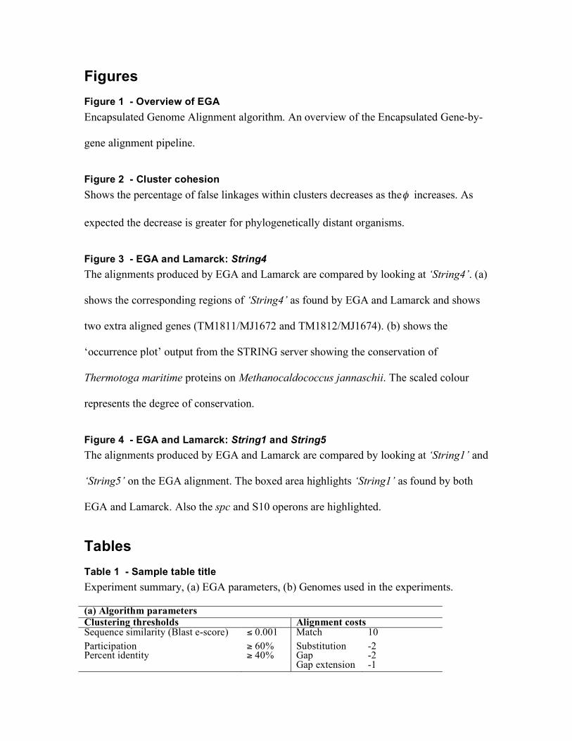
Figures

Figure 1 - Overview of EGA

Encapsulated Genome Alignment algorithm. An overview of the Encapsulated Gene-by-

gene alignment pipeline.

Figure 2 - Cluster cohesion

Shows the percentage of false linkages within clusters decreases as the! increases. As

expected the decrease is greater for phylogenetically distant organisms.

Figure 3 - EGA and Lamarck: String4

The alignments produced by EGA and Lamarck are compared by looking at ‘String4’. (a)

shows the corresponding regions of ‘String4’ as found by EGA and Lamarck and shows

two extra aligned genes (TM1811/MJ1672 and TM1812/MJ1674). (b) shows the

‘occurrence plot’ output from the STRING server showing the conservation of

Thermotoga maritime proteins on Methanocaldococcus jannaschii. The scaled colour

represents the degree of conservation.

Figure 4 - EGA and Lamarck: String1 and String5

The alignments produced by EGA and Lamarck are compared by looking at ‘String1’ and

‘String5’ on the EGA alignment. The boxed area highlights ‘String1’ as found by both

EGA and Lamarck. Also the spc and S10 operons are highlighted.

Tables

Table 1 - Sample table title

Experiment summary, (a) EGA parameters, (b) Genomes used in the experiments.

(a) Algorithm parameters Clustering thresholds Alignment costs Sequence similarity (Blast e-score) ! 0.001 Match 10

Participation " 60% Substitution -2 Percent identity " 40% Gap -2 Gap extension -1

(b) Nucleotide Protein Accessions M.tuberculosis H37Rv

4411532 3989 AL123456

M.leprae 3268203 1605 AL450380 L. Lai (Ch I /II) 4332241 / 358941 4360,367 AE010300, AE010301

L. Copenhageni (Ch I /II) 4277185 / 350181 3394,264 AE016823, AE016824

Table 2 - Sample table title

Sample comparison between the alignments produced by Lamarck and EGA. A * sign

indicates that EGA was not able to directly find this local alignment, however, looking at

the PHOGs it is easy to map the corresponding gene. The ** indicated that the EGA and

Lamarck alignments differed. String 4 shows the extended aligned segment found in the

EGA alignment.

Lamarck EGA T.maritima M. jannaschii T. maritima M. jannaschii Gene Gene Gene (PHOG) Gene (PHOG)

‘String1’ TM1480 MJ0478 15644228(925) 15668655(925) TM1481 MJ0477 15644229(926) 15668654(926) TM1482 MJ0476 15644230(927) 15668653(1464) TM1483 MJ0475 15644231(928) 15668652(928) TM1484 MJ0474 15644232(929) 15668651(929) - MJ0473 - 15668650(1463) - MJ0472 - 15668649(1462) TM1485 MJ0471 15644233(930) 15668648(930) TM1486 MJ0470 15644234(931) 15668647(931) TM1487 MJ0469 15644235(932) 15669881(932) TM1488 MJ0468 15644236(933) 15668646(933) missing - 15668645(1461) TM1489 MJ0467 15644237(934) 15668644(934) TM1490 MJ0466 15644238(935) 15668643(935) TM1491 MJ0465 15644239(936) 15668642(936) TM1492 MJ0464 - 15668641(1460) TM1493 MJ0463 15644240(937) 15668640(1459) - MJ0462 15644241(938) 15668639(1458) TM1494 MJ0461 15644242(939) 15668638(939) TM1495 MJ0460 15644243(940) 15668637(940) *‘String2’ TM0015 MJ0269 15642790(14) 15668443(14) TM0016 MJ0268 15642791(15) 15668442(15) TM0017 MJ0267 15642792(16) 15668441(16) TM0018 MJ0266 15642793(17) 15668440(17) **‘String3’ TM1261 MJ1012 15643822(25) 15669201(25) TM1262 MJ1013 15643823(26) 15669202(26) TM1263 MJ1014 15643824(27) 15669203(26) TM1264 MJ1015 - 15669204(1732) ‘String4’ TM1807 MJ1667 15644551(1144) 15669863(1144) TM1808 MJ1668 15644552(1145) 15669864(1145) TM1809 MJ1669 15644553(1146) 15669865(1146) TM1810 MJ1670 15644554(1147) 15669866(1147) extended region aligned by EGA - 15669867(2012) 15644555(13) 15669868(13) - 15669869(2013) 15644556(1148) 15669870(1148) *‘String5’ TM1496 MJ0180 15644244(941) 15668352(941)

TM1497 MJ0179 15644245(942) 15668351(942) TM1498 MJ0178 15644246(943) 15668350(943) TM1499 MJ0177 15644247(944) 15668349(1286) TM1500 MJ0176 15644248(945) 15668348(1285)

not found TM1502 15644250(947)

*‘String6’ TM1503 MJ1048 15644251(947) 15669237(947) TM1504 MJ1047 15644252(948) 15669236(948) TM1505 MJ1046 15644253(949) 15669235(949)

not found MJ1045 15669234(1745)

Additional files Additional file 1 – Clustering example

Protein sequences p (single domain d1) and q (two domains d

1 and d

2) are similar based

on domain d1. Another sequence r ( d

2 and d

3) maybe significantly similar to sequence

q based on domain d2. But a symmetric measure will link and cluster proteins p and r ,

which is inappropriate. This means that proteins p will only be added to a PHOG if there

is a protein q that is already a member of the PHOG such that S(p,q) " #cluster and the

proportion of both sequences involved in the alignment is greater than " .

Additional file 2 – EGA web server

A screenshot of the EGA server website showing the input form and explaining the

sample output containing the dot plot image and an extract from the alignment.

Additional file 3 – Dot plots of encapsulated genomes

EGA generated dot plots representing the encapsulated forms of the (a) L. serovar Lai

CHI vs. L. serovar Copenhageni CHI, (b) L. serovar Lai CHII vs. L. serovar

Copenhageni CHII and (c) M. tuberculosis vs. M. leprae. A point on the plot indicates

that the two proteins (x and y) are similar and belong to the same cluster. Point (0,0)

represents the origin of replication for both genomes.

Additional file 4 – Alignment significance

Assessing alignment significance through random permutations test. Significance of

alignment compared to 2000 randomized alignments of (a) Leptospira ser. Lai vs

shuffled Leptospira ser. Copenhageni (b) M. tuberculosis vs shuffled M. leprae. In both

the cases, the actual observed number of aligned clusters (444 and 853 respectively) lies

out of the random test distribution range, meaning that the probability of attaining the

observed number of aligned pairs or more by chance is less than 0.0005.

Additional table 1 – Clusters data

The table shows a summary of the cluster data for the experiments. For each experiment,

the table shows the number of clusters formed, containing proteins unique to 'genome 1'

(row 1) and 'genome2' (row 2). The number of clusters containing both genome 1 and

genome 2 proteins are mentioned in (row 3) and the size of the largest cluster is given in

the last row.

Comparisons

Proteins in M tub v M lep L. Lai v L. Cop ch I L. Lai v L. Cop ch II

genome 1 / genome 2 2189 / 207 1042 / 246 104 / 11

both genomes 1341 2945 249

largest cluster 25 66 4

Additional table 2 – EGA and Lamarck alignments

Available online from http://vbc.med.monash.edu.au/~kmahmood/EGA/lam.html. For

each pair of proteomes, the table shows the EGA alignment in (ega - EGA) and (ega.Lam

- Lamarck) formats as well as the actual Lamarck alignments from [16].

Ste

p1

. Sim

ila

rity

se

arc

hS

tep

2. C

lust

eri

ng

Ste

p3

. En

cap

sula

tio

n

Ge

no

me

1 +

Ge

no

me

2

(G1

)

(G2

)

Ste

p4

. Ali

gn

me

nt

- C

on

cate

na

te g

en

om

e

seq

ue

nce

s.

- C

alc

ula

te a

ll-a

ga

isn

t-a

ll

pa

irw

ise

sim

ilari

ty t

ab

le

(usi

ng

Bla

st)

- C

lust

er

sim

ilar

pro

tein

s.

- P

run

e o

n p

air

wis

e s

imi-

lari

ty s

ign

i�ca

nce

.

- P

run

e o

n a

lign

me

nt

id-

en

tity

e.g

. 70

%

- A

ssig

n a

clu

ste

r id

en

ti�

er.

- R

en

am

e e

ach

pro

tein

se

-

qu

en

ce w

ith

its

clu

ste

r id

-

en

ti�

er.

- C

rea

te n

ew

en

cap

sula

ted

seq

ue

ces

G1

` a

nd

G2

`

(ma

inta

inin

g g

en

e o

rde

r).

- A

lign

G1

` a

nd

G2

` u

sin

g

sta

nd

ard

dy

na

mic

pro

gra

mm

ing

alg

ori

thm

.

G1

G2

>gi|01|MDAEQNQEE.

..>gi|82|V

KAEPLKETETKQ...

>gi|03|DNLPRGSRA.

..... >gi|35|E

ERIKATMD...

>gi|12|SEAADPPAAA

...>gi|36|W

FLLKE......

G1

`

G2`

>CL1||MDAEQNQEE..

.>CL2||VK

AEPLKETETKQ...

>CL1||DNLPRGSRA..

.... >CL1||EE

RIKATMD...

>CL1||SEAADPPAAA.

..>CL5||WF

LLKE......

G1

`

G2`

CL1 CL2 CL1 - ...

| |

CL1 - CL1 CL5 ...

Figure1 Fig

ure

1

Th

erm

oto

ga

ma

ritima

(TM

)

Me

tha

no

cald

oco

ccus ja

nn

asch

ii

(MJ)

Strin

g4

- La

ma

rck

Strin

g4

- EG

A

Figure3(a)Th

erm

oto

ga

ma

ritima

(TM

)

Me

tha

no

cald

oco

ccus ja

nn

asch

ii

(MJ)

TM1810/

MJ1670

TM1809/

MJ1669

TM1811/

MJ1672

TM1806

TM1808/

MJ1668

TM1807/

MJ1667

TM1812/

MJ1674

TM1813

TM1814/

MJ0375

MJ1671

MJ1673

Figure3(b)Fig

ure

3

Part E, page 1.

Computational analysis of molecular coevolution in families of proteins Geoffrey I. Webb Faculty of IT Monash University Clayton, Vic, Australia Khalid Mahmood Jiangning Song James Whisstock Faculty of Medicine Monash University Clayton, Vic, Australia

Introduction One of the great challenges for biology in the coming century is to discover how biological processes emerge from the physical interactions of the building blocks of life. We investigate innovative computational techniques for understanding how molecular interactions give rise to protein function, one of the key foundations of life. Proteins are strings of molecules called amino acids. Each location within a protein is called a site. The string of amino acids for a protein is called its primary structure. In nature proteins fold into 3-dimensional conformations called their tertiary structure. Primary structure can be discovered from genomic data. However, theirtertiary structure is extremely difficult to discover creating a bottleneck towards uncovering their vastly important functional information. The computational techniques we design will significantly increase the amount of knowledge about protein structure and function that can be gleaned simply from primary protein sequence data alone. Various evolutionary and/or functional pressures result in variations between the amino acids at specific sites from protein to protein within a family. An established approach to analysing primary structure is to identify highly conserved sites – sites that are occupied by the same amino acid in most proteins in the family. Such sites usually play a critical role within the family, either structural or functional. Structural roles ensure that the protein adopts a required 3-dimensional conformation. Functional roles further play a part in the biological function that the protein performs. Amino acids often achieve their roles cooperatively through interaction with other sites in the protein, or with sites in other proteins. For example, to coordinate the ends of two loops may require at least two sites, one on either loop, with properties that are physiochemically compatible with one another. The cooperating amino acids need not be identical from protein to protein. All that is required is two or more sites with appropriate complementary properties. Such sites may not be highly conserved, but may nonetheless be identified computationally because there will be a clear pattern to the two sites. For example, when one is occupied by a positively charged amino acid the other might be occupied by one with a negative charge and vice versa. Thus, there will be coevolution of the sites – they may change from protein to protein, but such change will be accompanied by corresponding change at the other sites with which each interacts. The significance of this observation has led to a substantial body of research into identifying and exploiting coevolution within proteins [1-22]. Most of this research uses information theoretic approaches to identifying coevolution. We here present a powerful alternative, a machine learning approach using probabilistic and statistical techniques.

Part E, page 2.

Computational analysis of molecular coevolution Computational analysis of molecular coevolution within proteins is an area of increasing research that is demonstrating much promise [1-28]. Molecular coevolution occurs when there is a systematic relationship between evolutionary changes that occur at two or more sites, such as when one site changes from a residue (occurrence of an amino acid) with a positive charge to one with a negative charge, the other site changes to a residue with a complementary charge. The biological significance of coevolving sites is illustrated by the pioneering work of Lockless and Ranganathan [23] who identified through coevolutionary analysis a network of residues in the PDZ domain family of proteins that may be jointly responsible for the complex biological process of allosteric regulation. Application of a sequence-based statistical method on three distinct protein families further revealed that surprisingly small subsets of residues form physically connected networks that link functional sites in the protein [26]. Moreover, Lee et al. [27] designed a chimeric protein connecting a light-sensing signalling domain and successfully engineered the allosteric control based on statically identified coevolving sites. More recently, a subset of coevolving residues has been shown to determine the specificity of two-component signal transduction proteins (histidine kinase, HK and its cognate response regulator, RR) [28]. Moreover, the significance of coevolving residues has also been suggested in membrane proteins [25] where coevolving residues are frequently found within contiguous vicinity to helix-helix contacts. These initial break-throughs hold open the promise of new powerful computational tools to assist biologists understand the mechanisms by which proteins operate and hence better understand, and thus treat and prevent many biological processes including diseases and other medical conditions. Nevertheless, the potential functional and structural roles of these coevolving sites remain elusive and efficient computational techniques for identifying them are challenging and in great demand by biologists and medical researchers. Most current approaches to identifying coevolution within proteins operate on aligned primary sequence data, some relying on pure sequence data and other employing known structural information. The strings of amino-acids, one for each protein in a family, are aligned, often using standard multiple sequence alignment tools such as CLUSTAL [29]. These alignments identify the sites and assign each residue in each protein to a site. Some sites within some proteins are assigned to gaps, indicating that sites have been deleted or inserted from the protein. The residues at any pair of sites can then be examined for covariance. The Pearson’s chi-squared test for independence is the traditional statistical test for covariance in frequency data such as this. However, this test is unreliable when more than 10% of cells have frequencies below 5 [30]. As there are 441 (21x21 – 21 representing the 20 amino acids plus a value representing a gap) cells, this implies that more than 2000 (in practice, substantially more, because the amino acids have widely varying frequency) proteins would be required to obtain a reliable result. Many protein families contain fewer than 1000 members and hence clearly do not offer the potential to provide reliable assessments of covariance by these means. Instead, the usual approach is to use information theoretic measures, most commonly mutual information, or a variant thereof. One limitation of such measures is that they do not support tests for statistical significance – hence there is no objective criterion by which to select critical values of the measure at which to accept or reject the existence of coevolution. We hypothesise that these measures have high variance and hence low reliability. This is for the same reason that the chi-square test is unreliable with the quantities of data available (protein sequences for a family); there are so many parameters that the accumulation of small amounts of variance across each parameter can dominate the result.

A statistical alternative Our alternative approach is to consider the presence or absence of each amino acid at each site as a binary variable. We then test for covariance between each of the resulting 441 pairs of binary variables relating to the two sites. As negative correlation between one pair of these values

Part E, page 3.

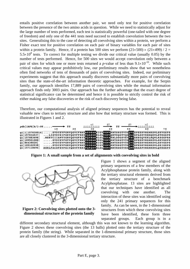
entails positive correlation between another pair, we need only test for positive correlation between the presence of the two amino acids in question. While we need to statistically adjust for the large number of tests performed, each test is statistically powerful (one-tailed with one degree of freedom) and only one of the 441 tests need succeed to establish coevolution between the two sites. Generalising this to the case of detecting all coevolving sites within a protein, we perform a Fisher exact test for positive correlation on each pair of binary variables for each pair of sites within a protein family. Hence, if a protein has 500 sites we perform (21×500) × (21×499) / 2 = 5.5×108 tests. To correct for multiple testing we divide our critical value (usually 0.05) by the number of tests performed. Hence, for 500 sites we would accept coevolution only between a pair of sites for which one or more tests returned a p-value of less than 9.1×10-10. While such critical values may appear prohibitively low, our preliminary results show that we nonetheless often find networks of tens of thousands of pairs of coevolving sites. Indeed, our preliminary experiments suggest that this approach usually discovers substantially more pairs of coevolving sites than the state-of-the-art information theoretic approaches. For example, for the Serpin family, our approach identifies 17,889 pairs of coevolving sites while the mutual information approach finds only 3003 pairs. Our approach has the further advantage that the exact degree of statistical significance can be determined and hence it is possible to strictly control the risk of either making any false discoveries or the risk of each discovery being false. Therefore, our computational analysis of aligned primary sequences has the potential to reveal valuable new clues to tertiary structure and also how that tertiary structure was formed. This is illustrated in Figures 1 and 2.

Figure 1: A small sample from a set of alignments with coevolving sites in bold Figure 1 shows a segment of the aligned primary sequences of a few members of the Acylphosphatase protein family, along with the tertiary structural elements derived from the tertiary structure of a benchmark Acylphosphatase. 13 sites are highlighted that our techniques have identified as all coevolving with one another. The interaction of these sites was identified using only the 241 primary sequences for this family. As can be seen, in the 1-dimensional structures from which these coevolving sites have been identified, these form three separated groups. Each group is in a

different secondary structural element, although this was not known to the learning algorithm. Figure 2 shows these coevolving sites (the 13 balls) plotted onto the tertiary structure of the protein family (the string). While separated in the 1-dimensional primary structure, those sites are all closely clustered in the 3-dimensional tertiary structure.

Figure 2: Coevolving sites plotted onto the 3-dimensional structure of the protein family

Part E, page 4.

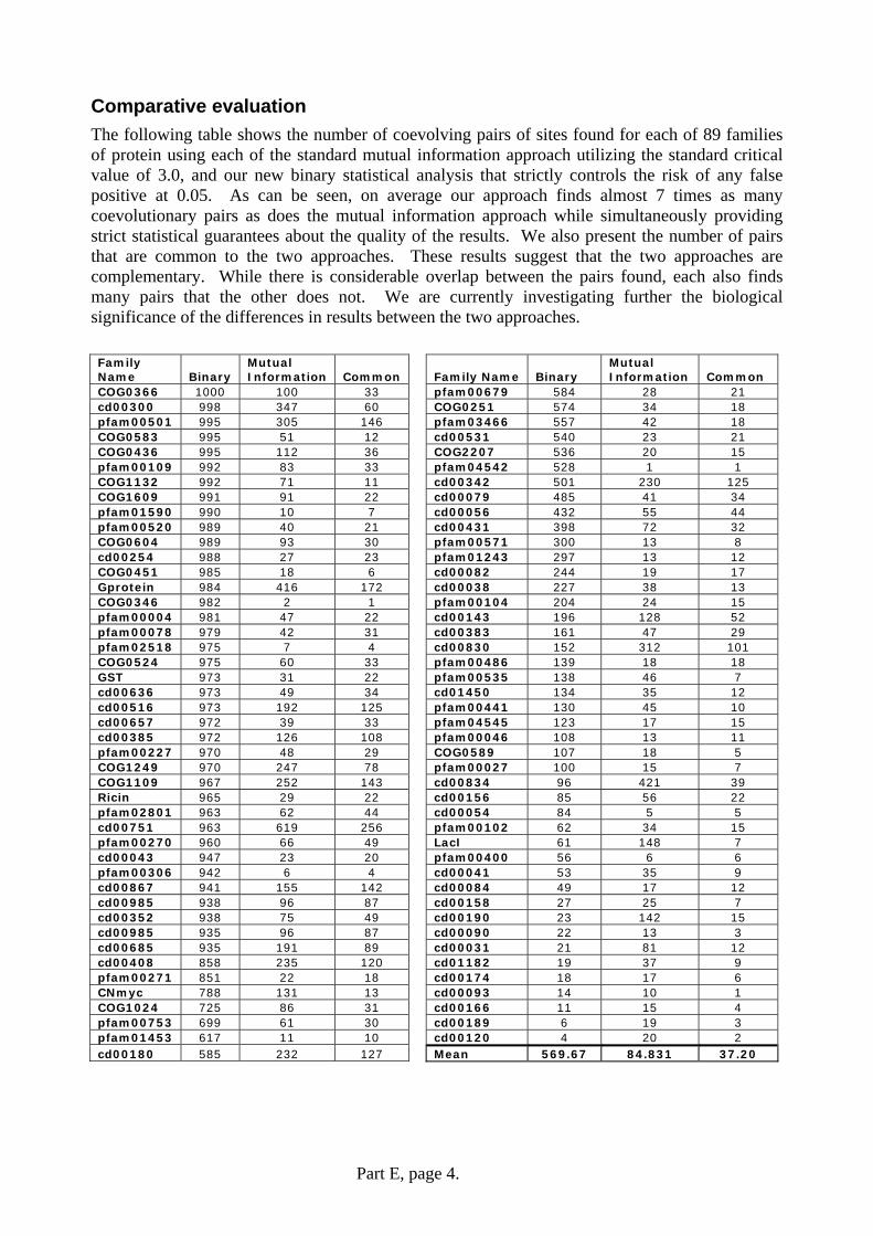
Comparative evaluation The following table shows the number of coevolving pairs of sites found for each of 89 families of protein using each of the standard mutual information approach utilizing the standard critical value of 3.0, and our new binary statistical analysis that strictly controls the risk of any false positive at 0.05. As can be seen, on average our approach finds almost 7 times as many coevolutionary pairs as does the mutual information approach while simultaneously providing strict statistical guarantees about the quality of the results. We also present the number of pairs that are common to the two approaches. These results suggest that the two approaches are complementary. While there is considerable overlap between the pairs found, each also finds many pairs that the other does not. We are currently investigating further the biological significance of the differences in results between the two approaches. Family Name Binary

Mutual Information Common

Family Name Binary

Mutual Information Common

COG0366 1000 100 33 pfam00679 584 28 21 cd00300 998 347 60 COG0251 574 34 18 pfam00501 995 305 146 pfam03466 557 42 18 COG0583 995 51 12 cd00531 540 23 21 COG0436 995 112 36 COG2207 536 20 15 pfam00109 992 83 33 pfam04542 528 1 1 COG1132 992 71 11 cd00342 501 230 125 COG1609 991 91 22 cd00079 485 41 34 pfam01590 990 10 7 cd00056 432 55 44 pfam00520 989 40 21 cd00431 398 72 32 COG0604 989 93 30 pfam00571 300 13 8 cd00254 988 27 23 pfam01243 297 13 12 COG0451 985 18 6 cd00082 244 19 17 Gprotein 984 416 172 cd00038 227 38 13 COG0346 982 2 1 pfam00104 204 24 15 pfam00004 981 47 22 cd00143 196 128 52 pfam00078 979 42 31 cd00383 161 47 29 pfam02518 975 7 4 cd00830 152 312 101 COG0524 975 60 33 pfam00486 139 18 18 GST 973 31 22 pfam00535 138 46 7 cd00636 973 49 34 cd01450 134 35 12 cd00516 973 192 125 pfam00441 130 45 10 cd00657 972 39 33 pfam04545 123 17 15 cd00385 972 126 108 pfam00046 108 13 11 pfam00227 970 48 29 COG0589 107 18 5 COG1249 970 247 78 pfam00027 100 15 7 COG1109 967 252 143 cd00834 96 421 39 Ricin 965 29 22 cd00156 85 56 22 pfam02801 963 62 44 cd00054 84 5 5 cd00751 963 619 256 pfam00102 62 34 15 pfam00270 960 66 49 LacI 61 148 7 cd00043 947 23 20 pfam00400 56 6 6 pfam00306 942 6 4 cd00041 53 35 9 cd00867 941 155 142 cd00084 49 17 12 cd00985 938 96 87 cd00158 27 25 7 cd00352 938 75 49 cd00190 23 142 15 cd00985 935 96 87 cd00090 22 13 3 cd00685 935 191 89 cd00031 21 81 12 cd00408 858 235 120 cd01182 19 37 9 pfam00271 851 22 18 cd00174 18 17 6 CNmyc 788 131 13 cd00093 14 10 1 COG1024 725 86 31 cd00166 11 15 4 pfam00753 699 61 30 cd00189 6 19 3 pfam01453 617 11 10 cd00120 4 20 2 cd00180 585 232 127 Mean 569.67 84.831 37.20

Part E, page 5.

Interpreting coevolution data. There has been considerable research into analysis of information derived from the identification of coevolution between sites. Our preliminary research suggests that coevolving sites tend to be grouped in close proximity in 3-dimensional space, so their identification using primary sequence data can provide important clues about tertiary structure as well as about functional interactions within the protein. However, coevolution is not restricted to sites that interact physically. Sites that are physically located at opposite sides of a folded protein can exhibit strong coevolution [23]. In fact, long-range coevolving residues can realize allosteric control by connecting the main functional sites (surface sites) with distantly positioned secondary sites, suggesting functional roles by these residues [23].

Open questions. While recently there has been much interest into methods for identifying molecular coevolution within protein families, there is limited understanding of how to direct this information to elucidate the biological operation of proteins. It would be useful to be able to distinguish coevolution due to phylogeny, physical interaction, cooperative function and structural role. Phylogenetic coevolution can occur when specific amino acids occupy specific sites in a protein high in the evolutionary tree. Unless there are evolutionary pressures to change either site, this configuration may be propagated to many of the ancestor’s descendents, creating phylogenetic coevolution. When sites are collocated, their physical interactions may result in evolutionary forces compelling residues to coevolve, even though these interactions do not play direct functional or structural roles. Biologists are usually most interested in coevolution resulting from sites performing functional or structural roles cooperatively. However, there has been limited progress in developing techniques to distinguish between these forms of coevolution.

Significance It is now relatively straightforward and cheap to determine the primary sequence of a protein through analysis of genomic data. It is extremely technically challenging, time consuming and expensive to determine and understand their tertiary structures. Our novel machine learning techniques hold the promise of revealing important clues to tertiary structure that may greatly aid various aspects from helping optimize their determination to their mutational and functional analysis. They also promise to increase the amount that can be determined about functional operation of a protein prior to determination of its tertiary structure. We have discovered an innovative new approach to identifying molecular coevolution by data mining primary sequence data. Its potential advantages over current methods include its greater statistical power and its ability to provide sound statistical significance levels to its predictions. Thus it should generate more complete and more reliable maps of coevolution within a protein family than the current state-of-the-art.

E8 REFERENCES 1. Atchley, W.R., et al., Correlations among amino acid sites in bHLH protein domains:. Molecular

Biology and Evolution, 2000. 17: 164-178. 2. Buck, M.J. & W.R. Atchley, Networks of coevolving sites in structural and functional domains of

serpin proteins. Molecular Biology and Evolution, 2005. 22: 1627-1634. 3. Codoner, F.M. & M.A. Fares, Why should we care about molecular coevolution? Evolutionary

Bioinformatics, 2008. 4: 29-38. 4. Dimmic, M.W., et al., Detecting coevolving amino acid sites using Bayesian mutational mapping.

Bioinformatics, 2005. 21: i126-i135. 5. Fares, M.A. & D. McNally, Coevolution analysis using protein sequences. Bioinformatics, 2006. 22:

2821-2822.

Part E, page 6.

6. Gloor, G.B., et al., Mutual information in protein multiple alignments reveals two classes of coevolving positions. Biochemistry, 2005. 44: 7156-7165.

7. Goh, C.S. & F.E. Cohen, Coevolutionary analysis reveals insights into protein-protein interactions. Journal of Molecular Biology, 2002. 324: 177-192.

8. Hamilton, N., et al., Protein contact prediction using patterns of correlation. Proteins, 2004. 56: 679-694.

9. Hoffman, N.G., C.A. Schiffer, & R. Swanstrom, Covariation of amino acid positions in HIV-protease. Virology, 2003. 314: 536-548.

10. Irving, J.A., et al., Phylogeny of the serpin superfamily: Implications of patterns of amino acid conservation for structure and function. Genome Research, 2000. 10(12): 1845-1864.

11. Jothi, R., et al., Coevolutionary analysis of domains in interacting proteins reveals insights into domain-domain interactions mediating protein-protein interactions. Journal of Molecular Biology, 2006. 362: 861-875.

12. Lichtarge, O., H.R. Bourne1, & F.E. Cohen, An evolutionary trace method defines binding surfaces common to protein families. Journal of Molecular Biology, 1996. 257: 342-358.

13. Madabushi, S., et al., Structural clusters of evolutionary trace residues are statistically significant and common in proteins. Journal of Molecular Biology, 2002. 316: 139-154.

14. Martin, L.C., et al., Using information theory to search for co-evolving residues in proteins. Bioinformatics, 2005. 21: 4116-4124.

15. Pollock, D.D. & W.R. Taylor, Effectiveness of correlation analysis in identifying protein residues undergoing correlated evolution. Protein Engineering, 1999. 6: 647-657.

16. Pollock, D.D., W.R. Taylor, & N. Goldman, Coevolving protein residues: Maximum likelihood identification and relationship to structure. Journal of Molecular Biology, 1999. 287: 187-198.

17. Pritchard, L., et al., Evaluation of a novel method for the identification of coevolving protein residues. Protein Engineering, 2001. 14: 549-555.

18. Raviscioni, M., et al., Correlated evolutionary pressure at interacting transcription factors and DNA response elements can guide the rational engineering of DNA binding specificity. Journal of Molecular Biology, 2005. 350: 402-415.

19. Tillier, E.R.M. & T.W.H. Lui, Using multiple interdependency to separate functional from phylogentic correlations in protein alignments. Bioinformatics, 2003. 19: 750-755.

20. Weckwerth, W. & J. Selbig, Scoring and identifying organism-specific functional patterns and putative phosphorylation sites in protein sequences using mutual information. Biochemical and Biophysical Research Communications, 2003. 307: 516-521.

21. Weigt, M., et al., Identification of direct residue contacts in protein-protein interaction by message passing. Proceedings of the National Academy of Sciences, 2009. 106(1): 67-72.

22. Kass, I. & A. Horovitz, Mapping pathways of allosteric communication in groEL by analysis of correlated mutations. Proteins: Structure, Function, and Genetics, 2002. 48(4): 611-617.

23. Lockless, S.W. & R. Ranganathan, Evolutionarily conserved pathways of energetic connectivity in protein families. Science, 1999. 286: 295-299.

24. Socolich, M., et al., Evolutionary information for specifying a protein fold. Nature, 2005. 437: 512-518.

25. Fuchs, A., et al., Co-evolving residues in membrane proteins. Bioinformatics, 2007. 23: 3312-3319. 26. Süel, G.M., et al., Evolutionarily conserved networks of residues mediate allosteric communication in

proteins. Nature Structural & Molecular Biology, 2003. 10: 59-69. 27. Lee, J., et al., Surface sites for engineering allosteric control in proteins. Science, 2008. 322: 438-442. 28. Skerker, J.M., et al., Rewiring the specificity of two-component signal transduction systems. Cell,

2008. 133(6): 1043-1054. 29. Altschul, S.F., et al., Gapped BLAST and PSI-BLAST: a new generation of protein database search

programs. Nucleic Acids Research, 1997. 25: 3389-3402. 30. Johnson, R., Elementary Statistics. 1984, Boston: Duxbury Press.

Association networks: A new approach to associationanalysis

Geoffrey I. WebbFaculty of IT

Monash UniversityClayton, Vic, Australia

webb@infotech.monash.edu.au

Khalid MahmoodFaculty of MedicineMonash University

Clayton, Vic, Australia{Khalid.Mahmood|Jiangning.Song}@med.monash.edu.au

Jiangning SongFaculty of MedicineMonash University

Clayton, Vic, Australia

ABSTRACTAssociation Networks provide a new type of association anal-ysis, revealing large scale grouping of items or attribute-values of a form that is not otherwise readily identified.They group all items that are connected by a chain of statis-tically significant pairwise associations. We present evidencethat this new technique can reveal high-level structure indata that cannot readily be exposed by previous unsuper-vised approaches. This type of analysis complements thenumerous fine-grained local interactions typically identifiedby association rule and itemset discovery.

Categories and Subject DescriptorsH.2.8 [Database Management]: Database Applications—data mining ; I.2.6 [Artificial Intelligence]: Learning; H.3.3[Information Storage and Retrieval]: Information Searchand Retrieval

KeywordsAssociation Discovery, Association Rules, Itemset Discovery,Interesting Itemsets

1. INTRODUCTIONAssociation discovery is a fundamental data mining task.

The predominant approach is Association Rule Discovery [2,3]. However, in many applications the organization of asso-ciations into antecedents and consequents has no value andserves only to obfuscate the relevant insight. An associationbetween a and b gives rise to two rules, a → b and b → aand an association between three items a, b and c can giverise to six rules, including a → b, a → b, c and a, b → c. Asthe number of items that are all positively associated withone another rises, the number of rules generated from theset often increases exponentially, but may reveal no furtherinformation than the existence of positive associations be-tween all the items. An obvious solution to this problemis to use itemsets as the reporting formalism, rather than

Permission to make digital or hard copies of all or part of this work forpersonal or classroom use is granted without fee provided that copies arenot made or distributed for profit or commercial advantage and that copiesbear this notice and the full citation on the first page. To copy otherwise, torepublish, to post on servers or to redistribute to lists, requires prior specificpermission and/or a fee.KDD ’09 Paris, FranceCopyright 200X ACM X-XXXXX-XX-X/XX/XX ...$5.00.

rules. An itemset is simply a set of items. There has beenmuch progress in the area of identifying potentially inter-esting itemsets [1, 2, 5, 6, 7, 9, 10, 11, 16, 17, 20, 21, 25,27, 31, 33]. There has been tremendous progress on efficienttechniques for finding all frequent itemsets [2, 13], and ef-fective techniques for finding subsets of these from which allfrequent itemsets can be recovered [5, 7, 12, 14, 20, 22, 26,32, 33]. However, frequent itemsets will be of little interestin many applications, as groups of frequent items can beexpected to form frequent itemsets irrespective of whetherthey are associated with one another [28].

A small number of techniques have been developed thatcan assess the potential interestingness of an itemset, butthey either require background knowledge [16] or are severelyconstrained with respect to the size of itemset they can pro-cess due to computational complexity that is exponential onthe itemset size [6, 10, 17, 31].

It turns out to be straightforward to identify associationpairs, pairs of items that pass a statistical significance testfor positive association. These are an attractive representa-tion for associations because they are easy to identify andhave less redundancy than association rules, which may rep-resent each association pair with two rules. However, it isdifficult to use them to identify higher-order interactions be-tween items. Further, some datasets result in generation ofvery large numbers of association pairs, up to 282,000 in theexperiments we present below. This can make it extremelydifficult for an end user to extract useful insights due simplyto the overwhelming quantity of information to process.

In this paper we present Association Networks, a newtechnique for summarizing and extracting high-level insightsfrom association pairs. We demonstrate that associationnetworks

• can provide novel forms of insight into the structurethat underlies a dataset, specifically by revealing high-level structure that complements the local interactionstypically revealed by existing association discovery tech-niques;

• are straightforward to interpret; and

• can be generated in a computationally efficient man-ner.

When generating association networks it is natural to alsoreport items that participate in no associations. This infor-mation appears also to often be valuable. It is surprisingthat this simple analysis does not appear to have a standardplace in association analysis practice, especially given the

large numbers of items that have no associations for somelarge datasets, as many as 14,000 in the datasets we inves-tigate.

This paper is organized as follows. We first provide aproblem statement, in which we define relevant terminology.We then define association networks and provide two moti-vating examples. This is followed by a discussion of com-putational considerations relating to identifying associationnetworks. Next we assess the performance of the approachon 10 datasets used in previous research. This is followed bya discussion of methods for limiting the networks to includeonly stronger associations. We finish by discussing relatedresearch and presenting our conclusions.

2. PROBLEM STATEMENTA dataset D is an n × m vector. Each of the n rows

represents an object of interest and each of the m columnsrepresents an attribute of the objects. For transactionaldata, each column represents an item and the entry for arow indicates the presence or absence of that item. In thecontext of transactional data, following the tradition of theresearch community, only associations involving the pres-ence of an item are considered. For attribute-value data,each attribute Ai has a domain of values dom(Ai), and eachentry in the column corresponding to that attribute has asingle value from that domain. We use the terms item andattribute-value interchangeably, to represent the base unit ofanalysis, be it either attribute-value or transactional data.

The association discovery task is to find interesting asso-ciations between combinations of values in differing columnsof D. Which associations will be interesting will vary greatlydepending upon the specific analytic task. It is not crediblethat any one criterion will identify exactly the associationsthat will prove interesting for all analytic objectives, butsome criteria may prove useful for a wide range of objec-tives.

There is a subtle but important difference between theobjectives of finding interesting associations and of findinginteresting correlations between variables. The latter hasbeen widely studied in statistics [24, 4] and is representedby Bayesian Network [15, 19] and Markov Random Field [8]discovery in the data mining community. Association dis-covery seeks interactions between specific attribute-valuesrather than between variables as a whole. This is the specificfocus of many real-world analytic tasks. For example, whenidentifying the primary customer segment for a product, weare interested not only in whether there is a correlation be-tween age and propensity to buy, but also in which specificage groups have raised propensity to purchase.

3. ASSOCIATION NETWORKSMost approaches to association discovery have sought to

discover either rules or itemsets. An itemset is a set ofattribute-values that are positively associated with one an-other. Association rules indicate an association between twosets of attribute-values. As indicated in the introduction,association rules introduce two roles, antecedent and conse-quent, that may be uninformative and may introduce large-scale redundancy into the set of rules that are found. Item-sets either represent only those combinations of attribute-values that co-occur frequently, which may not be of interestas frequent attribute-values should be expected to co-occur

with each other frequently, or are limited in their capacity todeal with interactions between large numbers of attributes.

This paper presents a new approach to analyzing associ-ations and seeks to establish that it has value in a range ofanalytic tasks. The intention is to augment rather than toreplace existing techniques.

Association networks are formed from association pairs.These are pairs of attribute-values that are positively cor-related. In the current work we detect association pairs bysubjecting every pair of attribute-values Ai=v and Aj=wsuch that i 6= j, v ∈ dom(Ai) and w ∈ dom(Ak) to a Fisherexact test, a statistical hypothesis test for correlation.

The p value for this test can be calculated as follows. Leta, b, c and d be, respectively the frequencies with which Ai=vand Aj=w co-occur, Ai=v occurs without Aj=w, Aj=woccurs without Ai=v, and neither Ai=v nor Aj=w occurs.

p =

min(b,c)∑

i=0

(a+b)!(c+d)!(a+c)!(b+d)!

(a+b+c+d)!(a+i)!(b−i)!(c−i)!(d+i)!. (1)

n! denotes the factorial of n.To control the risk of false discoveries [28], we use a Bon-

ferroni correction. This first requires calculation of the sizeof the search space, s.

s =m

∑

i=1

|dom(Ai)| ×m

∑

j=1,j 6=i

| dom(Aj)|

/2 (2)

where | · | denotes the cardinality of a set.To guarantee that the risk that any of the association pairs

found will be a false discovery shall be no greater than α,we accept only association pairs that achieve a significancelevel

p < α/s. (3)

In the current research we use α = 0.05.Our association pairs differ from Brin et. al.’s Generalized

Association Rules [6] by using the Bonferroni correction tocontrol false discoveries, as well as the more minor differ-ences of being limited to pairs and using an exact statisticaltest rather than the chi-squared test.

We denote the set of all association pairs by P .An association chain chain(Ai=v, Aj=w) exists betweentwo attribute-values Ai=v and Aj=w if and only if{Ai=v, Aj=w} ∈ P or ∃Ak=x, {Ai=v, Ak=x} ∈ P andchain(Ak=x, Aj=w). A set of attribute-values C is a can-didate network if and only if ∀Ai=v, Aj=w ∈ C, Ai=v =Aj=w ∨ chain(Ai=v, Aj=w). A candidate network is anassociation network if and only if it is not a subset of anyother candidate network.

We also identify items that are not in any association pair,as it turns out to often be revealing to discover which itemsdo not appear to participate in any form of association withany other item.

Association networks are fundamentally different to stan-dard approaches to identifying interesting itemsets. Inter-esting itemsets are usually sets of items that co-occur withunexpected frequency. Association networks are maximalcollections of items that form a connected network of asso-ciations.

We illustrate association networks using the well-knowniris dataset. Iris contains 150 records, each listing 5 proper-ties of an Iris flower: sepal-length, sepal-width, petal-length,

Table 1: Association Networks for the Iris data

sepal-length<5.4, sepal-width>3.2, petal-

length<3.0, petal-width<1.0, species=Iris-Setosa

5.4<=sepal-length<=6.3, sepal-width<2.9,

3.0<=petal-length<=4.9, 1.0<=petal-width<=1.6,

species=Iris-Versicolor

sepal-length>6.3, 2.9<=sepal-width<=3.2, petal-

length>4.9, petal-width>1.6, species=Iris-Viginica

petal-width and species. The first four attributes are nu-meric and the last is categorical with the three values iris-setosa, iris-versicolor and iris-viginica. This dataset was cre-ated as a testbed for classification learning. It contains 50examples of each species.

We performed association network analysis using the soft-ware tool Magnum Opus [30] with its default settings. Bydefault the software discretizes numeric variables into ter-ciles, the lower, middle and upper thirds of the distribution.Given this discretization, we find the three association net-works in Table 1.

These association networks find known structure in thedata, its division into three species. It reveals that Iris Se-tosa is associated with short wide sepals and small petals,Iris Versicolor is associated with mid-length narrow sepalsand mid-sized petals and Iris Viginica is associated with longmedium width sepals and large petals.

This illustrates the difference between association net-works and Bayesian networks or Markov random fields. Thelatter two approaches may discover that all five variablesare inter-related, but would not clearly reveal the inter-relationships between variable values shown here.

It also illustrates the difference between association net-works and itemset discovery techniques. Each of the net-works is an itemset, but they do not cover all the data. 22out of the 50 examples of Iris Setosa satisfy the first set ofitems, 19 out of 50 Iris Versicolor examples are covered bythe second and 18 out of 50 Iris Viginica examples are cov-ered by the last. We are not aware of any itemset discoverytechnique that would clearly highlight these groupings aboveall of their numerous subsets. However, they do appear tosuccinctly capture known structure in the data.

Another interesting example comes from the Breast Can-cer Wisconsin dataset, which relates to clinical diagnosis ofbreast cancer from pathology results. This data has tenattributes (not including a sample code number which isexcluded from this analysis), of which 9 have integer valuesbetween 1 and 10 and the remaining class attribute has 2 in-teger values, 2=benign and 4=malignant. Note that none ofthe attributes have been discretized because some are clearlycategorical in nature and we do not have the expertise todetermine which would appropriately be treated as ordinal.For this data the technique identifies 3 networks. A smallnetwork is associated with benign (class=2). A larger net-work is associated with malignant (class=4). This networkis larger because it includes more values for many of the at-tributes. A third network identifies two attribute-values thatare associated with one another but are not associated withany other values. Finally, 26 attribute-values are identifiedas each not being associated with any other value.

The simplicity of the structure revealed in these two exam-ples is refreshing in comparison to the unstructured massesof rules or itemsets that most association analysis techniquesreturn.

We need to be cautious, however, in assessing such a tech-nique’s utility by its ability to capture known structure. It isreassuring that it can reveal known structure, but its valuewill lie in its capacity to uncover previously unknown struc-ture in data. In the above example it has revealed classesthat are already known, but this is not its primary purpose.It is an unsupervised technique and so should have the ca-pacity to identify previously unknown classes in the data. Ifwe wish to discover structure associated with pre-identifiedclasses we should probably utilize an appropriate descriptivesupervised rule discovery technique [18].

4. COMPUTATIONAL CONSIDERATIONSThe first step in finding the association pairs is to find

all the counts for individual attribute-values and pairs of at-tribute values. This can be achieved in a single scan throughthe data requiring O(nm2) computations.

The discovery of association pairs from the summary ofpairwise counts in the worst case requires a Fisher exacttest be performed for each pair of values. Eq. 2 gives thenumber of tests to be performed. The Fisher exact test hasa reputation for being computationally expensive. However,all it requires is a number of simple arithmetic operations ona number of factorial values. The complexity of calculatingthe factorial of a value i is O(i). A total of 9 factorials haveto be calculated and manipulated a number of times whichis bounded by the number of objects in the data n. Themaximum value for which a factorial need be calculated isalso n. Hence the worst case complexity of a Fisher exacttest is O(n2). It follows that the worst case complexity offinding the association pairs is the complexity of the Fisherexact test times the number of pairs to be tested, whichequals O(n2 ∑m

i=1(|dom(Ai)| ×∑m

j=1,j 6=i|dom(Aj)|)). This

dominates the cost of finding the counts, which can thus bediscounted. If we consider the total number of attribute-values t

t =m

∑

i=1

|dom(Ai)| (4)

we can see that the worst case complexity is bounded byO(n2t2).

Once we have the association pairs, generating the net-works is straightforward. Our algorithm is presented in Ta-ble 3. Its worst case complexity is O(t2). Hence the worstcase complexity for the full process of discovering associationnetworks is bounded by O(n2t2).

5. ASSESSMENTTo assess the technique we applied it to the ten large

datasets we have previously used in association discoveryresearch [28, 29]. These data sets are described in Table 4.Numeric attributes were discretized into terciles as describedin Section 3, above.

We present first some simple quantitative descriptivestatistics listed in Table 5. We show for each dataset thenumber of association pairs found, the number of associ-ation networks extracted from those pairs, the minimum,maximum and mean size of those networks, and the number

Table 2: Association Networks for the Breast Cancer Wisconsin data

Clump Thickness=1, Clump Thickness=2, Clump Thickness=3, Uniformity of Cell Size=1, Uniformity of Cell

Shape=1, Marginal Adhesion=1, Single Epithelial Cell Size=1, Single Epithelial Cell Size=2, Bare Nuclei=1,

Bland Chromatin=1, Bland Chromatin=2, Normal Nucleoli=1, Mitoses=1, Class=2

Clump Thickness=7, Clump Thickness=8, Clump Thickness=9, Clump Thickness=10, Uniformity of Cell Size=3,

Uniformity of Cell Size=4, Uniformity of Cell Size=5, Uniformity of Cell Size=6, Uniformity of Cell

Size=7, Uniformity of Cell Size=8, Uniformity of Cell Size=10, Uniformity of Cell Shape=4, Uniformity of

Cell Shape=5, Uniformity of Cell Shape=6, Uniformity of Cell Shape=7, Uniformity of Cell Shape=8, Unifor-

mity of Cell Shape=10, Marginal Adhesion=4, Marginal Adhesion=5, Marginal Adhesion=6, Marginal Adhesion=7,

Marginal Adhesion=8, Marginal Adhesion=10, Single Epithelial Cell Size=3, Single Epithelial Cell Size=4,

Single Epithelial Cell Size=5, Single Epithelial Cell Size=6, Single Epithelial Cell Size=8, Single Ep-

ithelial Cell Size=10, Bare Nuclei=8, Bare Nuclei=10, Bland Chromatin=4, Bland Chromatin=5, Bland Chro-

matin=7, Bland Chromatin=8, Bland Chromatin=9, Bland Chromatin=10, Normal Nucleoli=3, Normal Nucleoli=4,

Normal Nucleoli=5, Normal Nucleoli=6, Normal Nucleoli=8, Normal Nucleoli=9, Normal Nucleoli=10, Mitoses=2,

Mitoses=3, Mitoses=4, Mitoses=10, Class=4

Uniformity of Cell Size=2, Uniformity of Cell Shape=2

26 items that are not in any association

Clump Thickness=4, Clump Thickness=5, Clump Thickness=6, Uniformity of Cell Shape=3, Uniformity of Cell

Shape=9, Marginal Adhesion=2, Marginal Adhesion=3, Marginal Adhesion=9, Single Epithelial Cell Size=7,

Single Epithelial Cell Size=9, Bare Nuclei=2, Bare Nuclei=3, Bare Nuclei=4, Bare Nuclei=5, Bare Nuclei=6,

Bare Nuclei=7, Bare Nuclei=9, Bland Chromatin=3, Bland Chromatin=6, Normal Nucleoli=2, Normal Nucleoli=7,

Mitoses=5, Mitoses=6, Mitoses=7, Mitoses=8, Mitoses=9

Table 4: Datasets

Dataset Records Items Minsup Description

BMS-WebView-1 59,602 497 60 E-commerce clickstream dataCovtype 581,012 125 359,866 Geographic forest vegetation dataIPUMS LA 99 88,443 1,883 42,098 Census dataKDDCup98 52,256 4,244 43,668 Mailing list profitability dataLetter Recognition 20,000 74 1,304 Image recognition dataMush 8,124 127 1,018 Biological dataRetail 88,162 16,470 96 Retail market-basket dataShuttle 58,000 34 878 Space shuttle mission dataSplice Junction 3,177 243 244 Gene sequence dataTICDATA 2000 5,822 709 5,612 Insurance policy holder data

Table 5: Quantitative statistics on association networks found

Dataset Pairs Networks Min. Max. Mean Unassoc.

BMS-WebView-1 18,637 3 2 465 156.7 26Covtype 2970 1 123 123 123 1IPUMS LA 99 29,492 11 2 1392 128.4 461KDDCup98 282,687 14 2 5604 402.6 14,024Letter Recognition 691 1 74 74 74 0Mush 1725 1 117 117 177 9Retail 10,408 434 2 3184 10.1 12,105Shuttle 184 1 34 34 34 0Splice Junction 466 4 2 205 53.3 29TICDATA 2000 7149 14 2 494 38.1 155

Table 3: Algorithm for finding association networks

- find association networks from association pairs- each item is denoted by a unique integer

Algorithm FindNet

Input:

n - an integer - the number of itemspaired[1..n,1..n] - a boolean array that is true iff two

items form an association pairOutput:

networks - a set of sets of items- each set of items is an association network

isolates - a set of items, each of which participates inno association pairs

begin

q[1..n] is initialized to the values 1..n - the queue of itemsto be processed

s := 1 - the index of the start of the current networke := 1 - the index of the end of the current network

for i := 1 to nfor j := e+1 to n

if paired[i,j] then

- found a new membere := e+1 - extend the networkswap(q[e+1], q[j]) - move the new member

into the networkend

end

if e = i then

- no more items to be added to the networkif e = s then

- the item is not paired with any other itemadd q[e] to isolates

else

add q[s..e] to networksend

s := i+1e := i+1

end

end

end

of attribute-values that were not in any association pair.For 4 of the 10 datasets, only one association network is

found. In two cases, this sole network includes all items. Forthese two datasets only minimal insight is derived — thatthe associations within the data are pervasive and tightlycoupled. For 2 of the 4, a number of items are not as-sociated with any other items, and this is potentially usefulinformation that, surprisingly, we are not aware of any otheranalysis technique revealing.

For the remaining 6 datasets substantial structure is re-vealed. In most cases there is one large network and a num-ber of smaller networks. Not being domain experts we havelimited capacity to assess the possible value of the informa-tion revealed. From our limited understanding the followingoutcomes appear potentially interesting.

For the BMS-Webview-1 click stream data, while most ofthe pages visited form a single network, there are two smallnetworks that are isolated from the main network: {a275,a276} and {a472, a474, a475}. That each of these consistsof locations in near sequential order suggests that an expertwould be able to readily find a reason for their connectednesswith one another. It is also potentially interesting that 26pages are each not associated with any other page.

For the KDDCUP98 data once again a large number ofitems form a single network. 13 further networks each con-tain between 2 and 5 items. Interestingly, the majority ofitems do not participate in any associations. This may be aresult of a need to aggregate items in this data, for example,to aggregate individual postcodes into higher-level regions.

The Retail data reveals the largest number of associationnetworks of all our datasets. This market-basket data hasbeen de-identified — items are identified by numeric codesonly. In consequence it is impossible to assess the potentialimport of any associations found without access to the en-coding used. The results are interesting, however, for thelarge amount of structure revealed by the association net-work analysis. Once again there is a single large network.The remaining 433 networks vary in size from 2 to 13 items.The majority of items are each not associated with any otheritem.

Splice Junction provides an interesting example of the po-tential for this approach to highlight novel and potentiallyuseful information. Again, the majority of items form a sin-gle network. This and the 3 remaining networks are shownin Table 6. These data relate to 60 site long strings of DNA.That two of the small association networks link values atsequential sites suggests that they would be open to readyinterpretation by a domain expert.

It is interesting to examine whether these networks mightbe revealed by existing itemset discovery techniques. Table 7shows the 16 itemsets formed from subsets of the associationnetwork S0=C, S1=T, S2=G, S3=G. Two measures, cover-age and leverage, are provided for each itemset. Each isreported as relative and absolute values, the latter in brack-ets. The absolute coverage is the number of examples thatcontain the itemset. The relative coverage is the proportionof all examples that contain the itemset. The absolute andrelative leverage are the respective coverage values less themaximum values that would be expected under an assump-tion of independence between any binary partition of theitems. For example, S0=C & S1=T & S2=G has a rela-tive coverage of 0.034. Its subset S1=T & S2=G has cover-age 0.084 and the remaining item S0=C has coverage 0.262.

Table 6: Association Networks for the Splice Junc-

tion data

S0=G, S1=A, S1=G, S1=C, S2=T, S2=C, S3=A, S3=T,

S3=C, S4=G, S4=T, S4=C, S5=G, S5=T, S5=C, S6=G,

S6=T, S6=C, S7=G, S7=T, S8=G, S8=T, S8=C, S9=A,

S9=G, S9=T, S9=C, S10=A, S10=G, S10=T, S10=C,

S11=G, S11=T, S11=C, S12=A, S12=G, S12=T, S12=C,

S13=A, S13=G, S13=T, S13=C, S14=T, S14=C, S15=A,

S15=G, S15=T, S15=C, S16=A, S16=G, S16=T, S17=A,

S17=G, S17=T, S17=C, S18=A, S18=G, S18=T, S18=C,

S19=A, S19=G, S19=T, S19=C, S20=A, S20=G, S20=T,

S20=C, S21=A, S21=G, S21=T, S21=C, S22=A, S22=G,

S22=T, S22=C, S23=A, S23=G, S23=T, S23=C, S24=A,

S24=G, S24=T, S24=C, S25=A, S25=G, S25=T, S25=C,

S26=G, S26=T, S27=A, S27=G, S27=T, S27=C, S28=A,

S28=G, S28=T, S28=C, S29=A, S29=G, S29=T, S29=C,

S30=A, S30=G, S30=T, S30=C, S31=A, S31=G, S31=T,

S31=C, S32=A, S32=G, S32=T, S32=C, S33=A, S33=G,

S33=T, S33=C, S34=A, S34=G, S34=T, S34=C, S35=G,

S35=T, S35=C, S36=G, S36=T, S36=C, S37=T, S37=C,

S38=A, S38=G, S38=T, S38=C, S39=A, S39=G, S39=T,

S39=C, S40=A, S40=G, S40=T, S40=C, S41=G, S41=T,

S41=C, S42=A, S42=G, S42=T, S42=C, S43=A, S43=G,

S43=T, S43=C, S44=G, S44=T, S44=C, S45=G, S45=C,

S46=A, S46=G, S46=T, S46=C, S47=G, S47=T, S47=C,

S48=G, S48=C, S49=A, S49=G, S49=T, S49=C, S50=A,

S50=G, S50=T, S50=C, S51=A, S51=G, S51=T, S51=C,

S52=G, S52=T, S52=C, S53=G, S53=T, S53=C, S54=G,

S54=C, S55=G, S55=T, S55=C, S56=A, S56=G, S56=T,

S56=C, S57=A, S57=G, S57=C, S58=G, S58=T, S58=C,

S59=G, S59=T, S59=C, class=EI, class=IE, class=N

S48=A, S52=A

S0=C, S1=T, S2=G, S3=G

S7=C, S8=A

Table 7: Itemsets for S0=C, S1=T, S2=G & S3=G

S0=C & S1=T [Coverage=0.084 (268); Leverage=0.0218

(69.3)]

S1=T & S2=G [Coverage=0.084 (268); Leverage=0.0213

(67.8)]

S2=G & S3=G [Coverage=0.084 (267); Leverage=0.0178

(56.5)]

S0=C & S1=T & S2=G [Coverage=0.034 (107); Lever-

age=0.0114 (36.2)]

S1=T & S2=G & S3=G [Coverage=0.027 (86); Lever-

age=0.0059 (18.8)]

S0=C & S2=G [Coverage=0.074 (236); Leverage=0.0050

(16.0)]

S0=C & S3=G [Coverage=0.067 (213); Leverage=0.0013

(4.0)]

S0=C & S1=T & S2=G & S3=G [Coverage=0.009 (30);

Leverage=0.0010 (3.2)]

{} [Coverage=1.000 (3177); Leverage=0.0000 (0.0)]

S2=G [Coverage=0.264 (839); Leverage=0.0000 (0.0)]

S0=C [Coverage=0.262 (833); Leverage=0.0000 (0.0)]

S3=G [Coverage=0.251 (797); Leverage=0.0000 (0.0)]

S1=T [Coverage=0.239 (758); Leverage=0.0000 (0.0)]

S0=C & S1=T & S3=G [Coverage=0.021 (67);

Leverage=-0.0001 (-0.2)]

S0=C & S2=G & S3=G [Coverage=0.021 (66);

Leverage=-0.0013 (-4.0)]

S1=T & S3=G [Coverage=0.056 (178); Leverage=-

0.0038 (-12.2)]

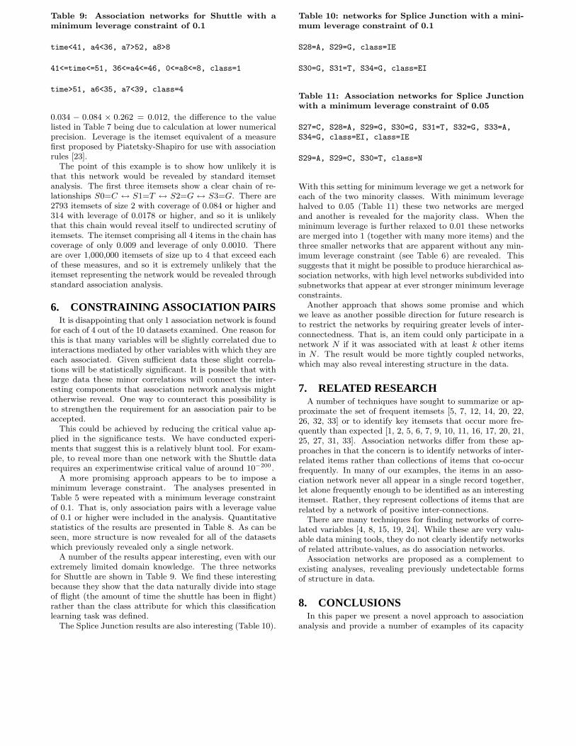
Table 9: Association networks for Shuttle with a

minimum leverage constraint of 0.1

time<41, a4<36, a7>52, a8>8

41<=time<=51, 36<=a4<=46, 0<=a8<=8, class=1

time>51, a6<35, a7<39, class=4

0.034 − 0.084 × 0.262 = 0.012, the difference to the valuelisted in Table 7 being due to calculation at lower numericalprecision. Leverage is the itemset equivalent of a measurefirst proposed by Piatetsky-Shapiro for use with associationrules [23].

The point of this example is to show how unlikely it isthat this network would be revealed by standard itemsetanalysis. The first three itemsets show a clear chain of re-lationships S0=C ↔ S1=T ↔ S2=G ↔ S3=G. There are2793 itemsets of size 2 with coverage of 0.084 or higher and314 with leverage of 0.0178 or higher, and so it is unlikelythat this chain would reveal itself to undirected scrutiny ofitemsets. The itemset comprising all 4 items in the chain hascoverage of only 0.009 and leverage of only 0.0010. Thereare over 1,000,000 itemsets of size up to 4 that exceed eachof these measures, and so it is extremely unlikely that theitemset representing the network would be revealed throughstandard association analysis.

6. CONSTRAINING ASSOCIATION PAIRSIt is disappointing that only 1 association network is found

for each of 4 out of the 10 datasets examined. One reason forthis is that many variables will be slightly correlated due tointeractions mediated by other variables with which they areeach associated. Given sufficient data these slight correla-tions will be statistically significant. It is possible that withlarge data these minor correlations will connect the inter-esting components that association network analysis mightotherwise reveal. One way to counteract this possibility isto strengthen the requirement for an association pair to beaccepted.

This could be achieved by reducing the critical value ap-plied in the significance tests. We have conducted experi-ments that suggest this is a relatively blunt tool. For exam-ple, to reveal more than one network with the Shuttle datarequires an experimentwise critical value of around 10−200 .

A more promising approach appears to be to impose aminimum leverage constraint. The analyses presented inTable 5 were repeated with a minimum leverage constraintof 0.1. That is, only association pairs with a leverage valueof 0.1 or higher were included in the analysis. Quantitativestatistics of the results are presented in Table 8. As can beseen, more structure is now revealed for all of the datasetswhich previously revealed only a single network.

A number of the results appear interesting, even with ourextremely limited domain knowledge. The three networksfor Shuttle are shown in Table 9. We find these interestingbecause they show that the data naturally divide into stageof flight (the amount of time the shuttle has been in flight)rather than the class attribute for which this classificationlearning task was defined.

The Splice Junction results are also interesting (Table 10).

Table 10: networks for Splice Junction with a mini-

mum leverage constraint of 0.1

S28=A, S29=G, class=IE

S30=G, S31=T, S34=G, class=EI

Table 11: Association networks for Splice Junction

with a minimum leverage constraint of 0.05

S27=C, S28=A, S29=G, S30=G, S31=T, S32=G, S33=A,

S34=G, class=EI, class=IE

S29=A, S29=C, S30=T, class=N

With this setting for minimum leverage we get a network foreach of the two minority classes. With minimum leveragehalved to 0.05 (Table 11) these two networks are mergedand another is revealed for the majority class. When theminimum leverage is further relaxed to 0.01 these networksare merged into 1 (together with many more items) and thethree smaller networks that are apparent without any min-imum leverage constraint (see Table 6) are revealed. Thissuggests that it might be possible to produce hierarchical as-sociation networks, with high level networks subdivided intosubnetworks that appear at ever stronger minimum leverageconstraints.

Another approach that shows some promise and whichwe leave as another possible direction for future research isto restrict the networks by requiring greater levels of inter-connectedness. That is, an item could only participate in anetwork N if it was associated with at least k other itemsin N . The result would be more tightly coupled networks,which may also reveal interesting structure in the data.

7. RELATED RESEARCHA number of techniques have sought to summarize or ap-

proximate the set of frequent itemsets [5, 7, 12, 14, 20, 22,26, 32, 33] or to identify key itemsets that occur more fre-quently than expected [1, 2, 5, 6, 7, 9, 10, 11, 16, 17, 20, 21,25, 27, 31, 33]. Association networks differ from these ap-proaches in that the concern is to identify networks of inter-related items rather than collections of items that co-occurfrequently. In many of our examples, the items in an asso-ciation network never all appear in a single record together,let alone frequently enough to be identified as an interestingitemset. Rather, they represent collections of items that arerelated by a network of positive inter-connections.

There are many techniques for finding networks of corre-lated variables [4, 8, 15, 19, 24]. While these are very valu-able data mining tools, they do not clearly identify networksof related attribute-values, as do association networks.

Association networks are proposed as a complement toexisting analyses, revealing previously undetectable formsof structure in data.

8. CONCLUSIONSIn this paper we present a novel approach to association

analysis and provide a number of examples of its capacity

Table 8: Quantitative statistics on association networks found with a minimum leverge constraint of 0.1

Dataset Pairs Networks Min. Max. Mean Unassoc.

BMS-WebView-1 0 0 496Covtype 11 6 2 3 2.7 108IPUMS LA 99 445 7 2 77 13.0 1782KDDCup98 2464 94 2 301 6.9 19,011Letter Recognition 8 4 2 4 2.8 62Mush 46 2 2 22 12.0 102Retail 0 0 16,469Shuttle 11 3 4 4 4.0 21Splice Junction 466 2 3 4 3.5 235TICDATA 2000 29 17 2 4 2.4 648

to identify potentially interesting structure in data of formsthat appear difficult to identify by existing means.

An association network is a maximal set of items thatare all connected to one another by a chain of associationsbetween items. Their detection is computationally tractableand their interpretation is straightforward.

A natural side-effect of association network discovery isidentification of all items that each are not associated withany other item. The identification of this group of items alsoappears to be potentially useful and we recommend it forconsideration for a place in every data miner’s basic toolkit.

Association networks are not a replacement for existingdata analysis techniques. However, we believe that they use-fully augment the numerous fine-grained interactions typi-cally identified by existing association discovery techniquesby exposing potentially interesting high-level structure indata of a form that is unlikely to be otherwise revealed.

9. ACKNOWLEDGMENTSThis research has been supported by Australian Research

Council grant DP0772238 and Air Force Office of ScientificResearch grant FA4869-07-1-4050 AOARD 074050.

We are grateful to Fei Zheng for useful feedback on a draftof this paper.

10. REFERENCES[1] C. Aggarwal and P. Yu. A new framework for item set

generation. In Prococeedings ACM-PODS Symposiumon Principles of Database Systems, pages 18–24, 1998.

[2] R. Agrawal, T. Imielinski, and A. Swami. Miningassociations between sets of items in massivedatabases. In Proceedings of the 1993 ACM-SIGMODInternational Conference on Management of Data,pages 207–216, Washington, DC, May 1993.

[3] R. Agrawal and R. Srikant. Fast algorithms for miningassociation rules. In M. J. Jorge B. Bocca andC. Zaniolo, editors, Proceedings of the 20thInternational Conference on Very Large DatabasesVLDB ’94, pages 487–499. Morgan Kaufmann,September 1994.

[4] A. Agresti. Categorical Data Analysis.Wiley-Interscience, New York, 2002.

[5] Y. Bastide, N. Pasquier, R. Taouil, G. Stumme, andL. Lakhal. Mining minimal non-redundant associationrules using frequent closed itemsets. In FirstInternational Conference on Computational Logic - CL2000, pages 972–986, Berlin, 2000. Springer-Verlag.

[6] S. Brin, R. Motwani, and C. Silverstein. Beyondmarket baskets: Generalizing association rules tocorrelations. In J. Peckham, editor, SIGMOD 1997,Proceedings ACM SIGMOD International Conferenceon Management of Data, pages 265–276, New York,NY, May 1997. ACM Press.

[7] T. Calders and B. Goethals. Mining all non-derivablefrequent itemsets. In Proceedings of the 6th EuropeanConference on Principles and Practice of KnowledgeDiscovery in Databases, PKDD 2002, pages 74–85,Berlin, 2002. Springer.

[8] R. Chellappa and A. Jain. Markov Random Fields:Theory and Application. Academic Press, 1993.

[9] R. Cooley, P.-N. Tan, and J. Srivastava. Discovery ofinteresting usage patterns from web data. InInternational WEBKDD-99 Workshop San Diego,pages 163–182, Berlin, 1999. Springer.

[10] W. DuMouchel and D. Pregibon. Empirical Bayesscreening for multi-item associations. In KDD-2001:Proceedings of the Seventh ACM SIGKDDInternational Conference on Knowledge Discovery andData Mining, pages 76–76, New York, NY, August2001. ACM Press.

[11] A. Fu, W. Renfrew, and J. Tang. Mining N-mostinteresting itemsets. In Proceedings of the 12thInternational Symposium on Foundations ofIntelligent Systems, pages 59–67, 2000.

[12] K. Gouda and M. J. Zaki. Efficiently mining maximalfrequent itemsets. In First IEEE InternationalConference on Data Mining, pages 163–170, San Jose,CA., November 2001.

[13] J. Han, J. Pei, and Y. Yin. Mining frequent patternswithout candidate generation. In Proceedings 2000ACM-SIGMOD International Conference onManagement of Data (SIGMOD’00), pages 1–12,Dallas, TX, May 2000.

[14] J. Han, J. Wang, Y. Lu, and P. Tzvetkov. Miningtop-K frequent closed patterns without minimumsupport. In International Conference on Data Mining,pages 211–218, 2002.

[15] D. Heckerman, D. Geiger, and D. M. Chickering.Learning Bayesian networks: The combination ofknowledge and statistical data. Machine Learning,20:197–243, 1995.

[16] S. Jaroszewicz and D. A. Simovici. Interestingness offrequent itemsets using Bayesian networks as

background knowledge. In R. Kohavi, J. Gehrke, andJ. Ghosh, editors, KDD-2004: Proceedings of theTenth ACM SIGKDD International Conference onKnowledge Discovery and Data Mining, pages178–186, New York, NY, August 2004. ACM Press.

[17] H. H. Malik and J. R. Kender. High quality, efficienthierarchical document clustering using closedinteresting itemsets. In Proceedings of the Sixth IEEEInternational Conference on Data Mining, pages991–996. IEEE, 2006.

[18] P. Novak, L. N, and G. Webb. Supervised descriptiverule discovery: A unifying survey of contrast set,emerging pattern and subgroup discovery. Journal ofMachine Learning Research, in press.

[19] J. Pearl. Probabilistic Reasoning in IntelligentSystems: Networks of Plausible Inference. MorganKaufmann Publishers, 1988.

[20] J. Pei, G. Dong, W. Zou, and J. Han. On computingcondensed frequent pattern bases. In Second IEEEInternational Conference on Data Mining (ICDM’02),pages 378–385, 2002.

[21] J. Pei, J. Han, and L. Lakshmanan. Mining frequentitemsets with convertible constraints. In Proceedings ofthe International Conference on Data Engineering,pages 433–442, 2001.

[22] J. Pei, J. Han, and R. Mao. CLOSET: An efficientalgorithm for mining frequent closed itemsets. InProceedings 2000 ACM-SIGMOD InternationalWorkshop on Data Mining and Knowledge Discovery(DMKD’00), pages 21–30, Dallas, TX, May 2000.

[23] G. Piatetsky-Shapiro. Discovery, analysis, andpresentation of strong rules. In G. Piatetsky-Shapiroand J. Frawley, editors, Knowledge Discovery inDatabases, pages 229–248. AAAI/MIT Press, MenloPark, CA., 1991.

[24] B. G. Tabachnick and L. S. Fidell. Using MultivariateStatistics. Allyn and Bacon, Boston, MA, 2001.

[25] N. Tatti. Maximum entropy based significance ofitemsets. Knowledge and Information Systems,17:57–77, 2008.

[26] C. Wang and S. Parthasarathy. Summarizing itemsetpatterns using probabilistic models. In Proceedings ofthe 12th ACM SIGKDD International Conference onKnowledge Discovery and Data Mining, pages730–735, 2006.

[27] J. Wang, J. Han, Y. Lu, and P. Tzvetkov. TFP: Anefficient algorithm for mining top-K frequent closeditemsets. In IEEE Transactions on Knowledge andData Engineering, pages 652–664, 2005.

[28] G. I. Webb. Discovering significant patterns. MachineLearning, 68(1):1–33, 2007.

[29] G. I. Webb. Layered critical values: A powerfuldirect-adjustment approach to discovering significantpatterns. Machine Learning, 71(2-3):307–323, 2008.Technical Note.

[30] G. I. Webb. Magnum Opus Version 4.3. Software, G.I. Webb & Associates, Melbourne, Aust., 2008.

[31] X. Wu, D. Barbara, and Y. Ye. Screening andinterpreting multi-item associations based onlog-linear modeling. In Proceedings of the Ninth ACMSIGKDD International Conference on KnowledgeDiscovery and Data Mining, pages 276–285, 2003.

[32] X. Yan, H. Cheng, J. Han, and D. Xin. Summarizingitemset patterns: A profile based approach. InProceedings of the Eleventh ACM SIGKDDInternational Conference on knowledge Discovery inData Mining, pages 314–323, 2005.

[33] M. J. Zaki and C. J. Hsiao. CHARM: An efficientalgorithm for closed itemset mining. In Proceedings ofthe Second SIAM International Conference on DataMining, pages 457–473, 2002.