A boosting method for maximization of the area under the ROC curve

Ann Inst Stat Math (2011) 63:961–979DOI 10.1007/s10463-009-0264-y

A boosting method for maximization of the areaunder the ROC curve

Osamu Komori

Received: 1 December 2008 / Revised: 8 July 2009 / Published online: 28 October 2009© The Institute of Statistical Mathematics, Tokyo 2009

Abstract We discuss receiver operating characteristic (ROC) curve and the areaunder the ROC curve (AUC) for binary classification problems in clinical fields. Wepropose a statistical method for combining multiple feature variables, based on aboosting algorithm for maximization of the AUC. In this iterative procedure, varioussimple classifiers that consist of the feature variables are combined flexibly into asingle strong classifier. We consider a regularization to prevent overfitting to data inthe algorithm using a penalty term for nonsmoothness. This regularization methodnot only improves the classification performance but also helps us to get a clearerunderstanding about how each feature variable is related to the binary outcome vari-able. We demonstrate the usefulness of score plots constructed componentwise by theboosting method. We describe two simulation studies and a real data analysis in orderto illustrate the utility of our method.

Keywords AUC · Boosting · Classification · ROC curve · Smoothing

1 Introduction

The receiver operating characteristic (ROC) curve has been widely used in medi-cal and biological sciences (Zhou et al. 2002; Pepe 2003), for applications in whichthe classification performance can be measured by the area under the ROC curve(AUC). This curve has three primary appealing properties. First, it does not assumeany specific distributional model, so a method based on the ROC is distribution-free, in contrast to logistic regression analysis or classical linear discriminant analysis

O. Komori (B)Department of Statistical Science, The Graduate University for Advanced Studies,Minami-azabu, Tokyo, 106-8569, Japane-mail: [email protected]

123

962 O. Komori

under normality assumption. Second, it is independent of the prior probabilities ofgroup membership, so it is able to accommodate case–control studies. Third, theAUC is not influenced by the choice of thresholds that may be changed according toeach decision-maker’s objective; hence, the AUC expresses the intrinsic accuracy ofclassification performance. The advantages of the AUC over the odds ratio or rela-tive risk when evaluating the classification performance are discussed by Pepe et al.(2004).

A procedure for maximizing the AUC using a linear combination of multiple fea-ture variables has been proposed (Pepe and Thompson 2000) in order to improve ondiagnostic accuracy of a single feature variable, and Pepe et al. (2006) have shown thatthe AUC-based method can be far superior to logistic regression in certain situations.Ma and Huang (2005) extended this strategy to high-dimensional data by adopting asigmoid approximation for the AUC. The assumption of linearity gives us easily inter-pretable results of the analysis, and allows us to get the rough characteristics of eachfeature variable. However, this strict assumption is often unable to capture informativenonlinear structures in the real world.

Moreover, it has been proved that the optimal combination of feature variables thatmaximizes the AUC is constructed based on the likelihood ratio (Eguchi and Copas2002; McIntosh and Pepe 2002). This implies that even under a simple setting such asa normality assumption with unequal covariance matrices, the optimal combination isnot linear but quadratic. Further details are described in Sect. 4.2.

In this paper, we propose a new statistical method to detect a more essential asso-ciation between feature variables and a binary outcome variable using a boostingtechnique, and apply the method to the combination of the feature variables for bet-ter classification. A typical one of the boosting methods is AdaBoost (Freund andSchapire 1997), which is designed to minimize the exponential loss. An AdaBoost-based boosting method for the AUC is presented by Long and Servedio (2007), alongwith its theoretical justification. The purpose of boosting methods is to construct astrong classifier by combining various weak classifiers. Recently, a variety of lossfunctions other than the exponential loss have been proposed and discussed in severalcontexts (Murata et al. 2004).

On the other hand, the generalized additive model (GAM) proposed by Hastie andTibshirani (1986) has wide applications in a variety of research fields. This is mainlybecause this model can detect the nonlinear effects of feature variables on the objectivefunction flexibly, without sacrificing interpretability:

η(E(y|x)) = F1(x1) + · · · + Fp(x p),

where x = (x1, . . . , x p)′, η is a link function and Fk , k = 1, . . . , p, are unspecified

functions of xk . Thus, GAM is also well suited for binary classifications in medicaland biological fields, in which the association of the feature vector x with an outcomevariable y is of great interest. We consider a model, similar to GAM, that attachesimportance to interpretability as well as flexibility, maximizing the AUC for a scorefunction F(x) by a boosting algorithm. As a result, we obtain F(x) of the form

F(x) = F1(x1) + · · · + Fp(x p),

123

A boosting method for maximization of the area under the ROC curve 963

in which we consider score plots of Fk(xk) against the kth feature variable xk . Theseplots are useful in association studies, for looking at how each feature variable worksin the classification and for detecting which feature variable is the most effective one.

This paper is organized as follows. In Sect. 2, we give a brief review of the ROCcurve and discuss the relationship between the AUC and the approximate AUC. InSect. 3, we propose AUCBoost, a new boosting method based on the maximizationof the AUC. In Sect. 4 we present two simple simulation studies to investigate theefficiency of AUCBoost, and in Sect. 5 we demonstrate the application of AUCBoostto a real data set. We close Sect. 6 with concluding remarks and ideas for future work.

2 Receiver operating characteristic curve

2.1 AUC

Let y be a binary class label (y = 0, 1), x ∈ Rp be a feature vector, and g0(x), g1(x)

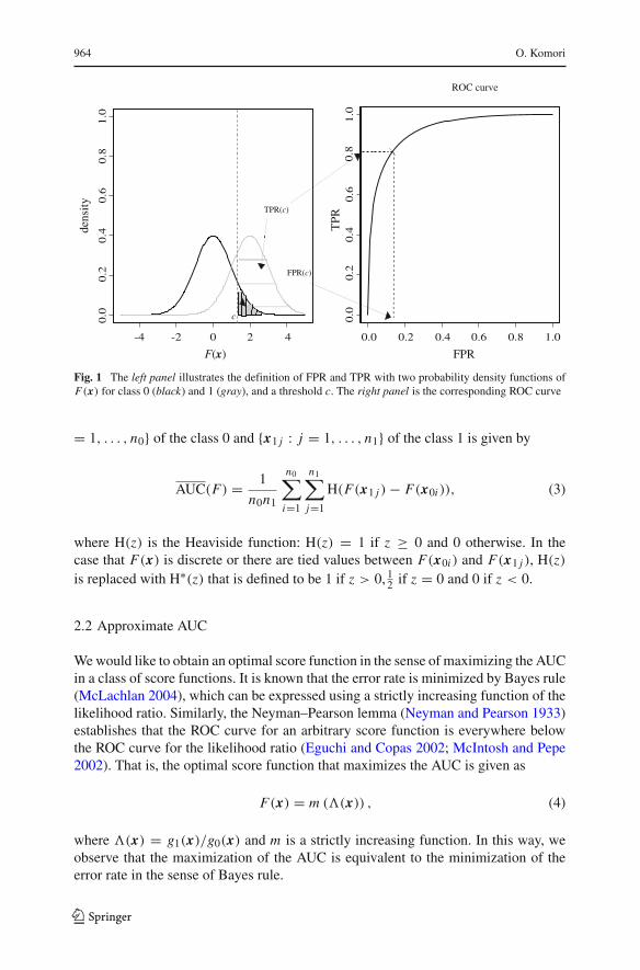
be probability density functions for each class. We classify a subject with feature vec-tor x into class 1 if a score function F(x) is greater than or equal to a threshold valuec, and into class 0 otherwise. Then, the false positive rate (FPR) and true positive rate(TPR) are defined as

FPR(c) =∫

F(x)≥cg0(x)dx and TPR(c) =

∫F(x)≥c

g1(x)dx. (1)

By pairing these probabilities, the ROC curve is given as

ROC = {(FPR(c), TPR(c)) |c ∈ R},

which is illustrated in Fig. 1.From (1), the AUC is written as

AUC(F) =∫ −∞

∞TPR(c)dFPR(c). (2)

The large separation of g0(x) and g1(x) could make the AUC close to 1. However,note that it is also dependent on a score function F(x), which we must determine in ananalysis of data. Only after employing an adequate F(x) for the two probability den-sity functions can we obtain the best value of the AUC. Equation (2) can be expressedin another manner:

AUC(F) = P(F(X1) ≥ F(X0)),

where X0, X1 are independent p-dimensional random vectors from class 0 and class1, respectively (Bamber 1975). The empirical AUC for given observations {x0i : i

123

964 O. Komori

-4 -2 0 2 4

F(x)

0.0

0.2

0.4

0.6

0.8

1.0

dens

ity

c

FPR(c)

TPR(c)

0.0 0.2 0.4 0.6 0.8 1.0

FPR0.0

0.2

0.4

0.6

0.8

1.0

TPR

ROC curve

Fig. 1 The left panel illustrates the definition of FPR and TPR with two probability density functions ofF(x) for class 0 (black) and 1 (gray), and a threshold c. The right panel is the corresponding ROC curve

= 1, . . . , n0} of the class 0 and {x1 j : j = 1, . . . , n1} of the class 1 is given by

AUC(F) = 1

n0n1

n0∑i=1

n1∑j=1

H(F(x1 j ) − F(x0i )), (3)

where H(z) is the Heaviside function: H(z) = 1 if z ≥ 0 and 0 otherwise. In thecase that F(x) is discrete or there are tied values between F(x0i ) and F(x1 j ), H(z)is replaced with H∗(z) that is defined to be 1 if z > 0, 1

2 if z = 0 and 0 if z < 0.

2.2 Approximate AUC

We would like to obtain an optimal score function in the sense of maximizing the AUCin a class of score functions. It is known that the error rate is minimized by Bayes rule(McLachlan 2004), which can be expressed using a strictly increasing function of thelikelihood ratio. Similarly, the Neyman–Pearson lemma (Neyman and Pearson 1933)establishes that the ROC curve for an arbitrary score function is everywhere belowthe ROC curve for the likelihood ratio (Eguchi and Copas 2002; McIntosh and Pepe2002). That is, the optimal score function that maximizes the AUC is given as

F(x) = m (�(x)) , (4)

where �(x) = g1(x)/g0(x) and m is a strictly increasing function. In this way, weobserve that the maximization of the AUC is equivalent to the minimization of theerror rate in the sense of Bayes rule.

123


In practice, the maximization of the empirical AUC presents some difficultiesbecause it consists of a sum of nondifferentiable functions, as seen in Eq. (3). Thisfeature prevents us from using gradient-based methods and requires a time-consumingsearch for the optimal score function (Pepe and Thompson 2000; Pepe et al. 2006).However, such a method becomes impossible to implement as the number of featurevariables increases greatly. Therefore, as a means of maximizing the empirical AUC,it has become common to use smooth-function approximations. Eguchi and Copas(2002) used the standard normal distribution function, and Ma and Huang (2005) pro-posed a sigmoid approximation for this purpose. In this paper, we consider the formerapproximation:

AUCσ (F) = 1

n0n1

n0∑i=1

n1∑j=1

Hσ (F(x1 j ) − F(x0i )),

where Hσ (z) = �(z/σ), with � being the standard normal distribution function. Asmaller scale parameter σ means a better approximation of the Heaviside functionH(z). The choice of the approximation function of H(z) does not matter so much; theimportant property is that the first derivative of the approximation function must besymmetric, which is satisfied in both Hσ (z) and the sigmoid function. This propertyis essential for the proof of Theorem 1.

Next, we discuss the relationship between the AUC and the approximate AUC. Wenote that the AUC for a score function F(x) has an integral formula given as

AUC(F) =∫∫

H(F(x1) − F(x0))g0(x0)g1(x1)dx0dx1.

Similarly, the approximate AUC is given as

AUCσ (F) =∫∫

Hσ (F(x1) − F(x0))g0(x0)g1(x1)dx0dx1.

Hence, we observe that AUCσ (F) almost surely converges to AUCσ (F) as n0 and n1both increase to infinity.

Theorem 1 Let

�(c) = AUCσ (F + c m (�)) ,

where �(x) = g1(x)/g0(x) and m is a strictly increasing function. Then, �(c) is astrictly increasing function of c ∈ R, and

supF

AUCσ (F) = limc→∞ �(c) = AUC (�) . (5)

123

966 O. Komori

Proof Let ζ(x) = m (�(x)). Then, the first derivative of �(c) with respect to c isgiven as

∫∫(ζ(x1)−ζ(x0)) H′

σ (F(x1) + c ζ(x1)−F(x0) − c ζ(x0)) g0(x0)g1(x1)dx0dx1,

which can be rewritten as

∫∫(ζ(x0)−ζ(x1)) H′

σ (F(x1)+c ζ(x1) − F(x0) − c ζ(x0)) g0(x1)g1(x0)dx1dx0,

by the exchange of x0 for x1 because of the symmetry: H′σ (−z) = H′

σ (z). Hence, weconclude that

2∂

∂c�(c) =

∫∫(ζ(x1) − ζ(x0)) H′

σ (F(x1) + cζ(x1) − F(x0) − c ζ(x0))

× g0(x0)g0(x1) (�(x1) − �(x0)) dx0dx1,

which is always positive because of the assumption that m is a strictly increasingfunction. Hence, the function �(c) is strictly increasing.

From the discussion above, it follows that

AUCσ (F) < limc→∞ �(c)

= limc→∞ AUCσ

[c

{F

c+ ζ

}]

= limc→∞ AUC σ

c

(F

c+ ζ

)

= AUC(ζ )

= AUC(�),

which concludes (5). �

From Theorem 1, we observe that

AUCσ (F) < AUC (�) ,

and that no score function F(x) can attain the equality above when σ > 0. Hence, wecan perform the supremization of AUCσ (F) instead of the maximization. This prop-erty is not preferable in building an iterative algorithm for maximization of AUCσ (F);therefore, we propose a regularization scheme for F(x) in a subsequent discussion.

123


3 AUCBoost

3.1 Objective function

We investigate a classification problem based on a boosting method. The key conceptis to construct a powerful score function F(x) by combining many various weak clas-sifiers (Hastie et al. 2001). Any single weak classifier itself has a very poor ability forclassification, whose performance is almost equal to random guessing; however, thecombination of a number of them produces a very flexible and strong score function.We aim to construct F(x) in such a way based on the AUC.

At first, we prepare a set Fk for each kth component of x ∈ Rp:

Fk = { f (x) = aH(xk − b) + (1 − a)/2 | a ∈ {−1, 1}, b ∈ Bk} , k = 1, . . . , p,

where Bk is a finite discrete set, which is determined by taking every intermediatepoint of samples or a number of sample quantiles. As seen in the definition, f (x) isa simple step function taking one of the two values {0, 1}. Then, we combine the setsinto

F =p⋃

k=1

Fk, (6)

called the decision stump class, among which we choose weak classifiers to con-struct F(x). The set F can be modified to include interaction terms that may improveclassification performance. However, the interpretation becomes difficult and unclearespecially when the number of feature variables is large. Hence, in this paper we focusonly on the main effects of feature variables.

In this setting, F(x) can be decomposed as the same way as GAM:

F(x) =∑f ∈F ′

1

α f f (x) + · · · +∑f ∈F ′

p

α f f (x)

= F1(x1) + · · · + Fp(x p),

where F ′k is a subset of Fk , k = 1, . . . , p, whose elements f ′s are selected in a boost-

ing algorithm in Sect. 3.2, and α f means a corresponding coefficient of f . Using thesenotations, the objective function we propose is given as

AUCσ,λ(F) = 1

n0n1

n0∑i=1

n1∑j=1

Hσ (F(x1 j ) − F(x0i ))

−λ

p∑k=1

∑xk∈Bk

{F (2)

k (xk)}2

, (7)

123

968 O. Komori

where λ is a smoothing parameter and F (2)k (xk) denotes the second-order difference

of Fk(xk): F (2)k (xk) = Fk(x (−1)

k ) − 2Fk(xk) + Fk(x (+1)k ) with x (−1)

k < x (+1)k . The

first term is the approximate empirical AUC based on the standard normal distribu-tion function; the second term gives a penalty for redundant behavior of F(x), whichfocuses on points in Bk for each k because Fk(xk) has discontinuities only at thepoints. Thus, the modeling of F(x) is similar to that of GAM. The difference is thatthe proposed method is based on maximization of the AUC in place of the likelihood,and that we use the second-order difference of Fk(xk) instead of the second derivativeof Fk(xk) because of its nonsmoothness. The iteration method is also different: wemaximize the objective function by a boosting method, whereas GAM is implementedby a backfitting algorithm (Hastie et al. 2001). We investigate the difference in detailusing numerical simulation data in Sect. 4.

We note that there is a special relation between the scale parameter σ and thesmoothing parameter λ. Equation (7) can be rewritten as

AUCσ,λ(F) = 1

n0n1

n0∑i=1

n1∑j=1

Hσ (F(x1 j ) − F(x0i ))

−λσ 2p∑

k=1

∑xk∈Bk

{F (2)

k (xk)

σ

}2

.

Hence, we have

AUCσ,λ(F) = AUCσ ′,λ′(

σ ′

σF

),

if λσ 2 = λ′σ ′2. This implies that the maximization of AUCσ,λ(F) is equivalent tothat of AUC1,λσ 2

( Fσ

). Therefore, we have

maxσ,λ,F

AUCσ,λ(F) = maxλ,F

AUC1,λ(F).

From this consideration, we can fix σ = 1 without loss of generality. Henceforth, wediscuss

AUCλ(F) = 1

n0n1

n0∑i=1

n1∑j=1

�(F(x1 j ) − F(x0i )) − λ

p∑k=1

∑xk∈Bk

{F (2)

k (xk)}2

,

which is rewrite of AUC1,λ(F) for notational convenience. This discussion not onlyleads to a drastic reduction of the computational cost for the implementation of ourmethod, but also has consistency with Theorem 1. The scale parameter σ , which con-trols the accuracy of the approximation of the AUC, is not an essential factor in thesense of the supremization of the approximate AUC. On the other hand, the smoothingparameter λ has another important role. As mentioned after Theorem 1, the approxi-mate AUC has no maximum in itself. The penalty term for smoothness in AUCλ(F)

123


also guarantees the existence of the maximum of AUCλ(F), and makes the numericalmaximization stable.

Ma and Huang (2007) and Wang et al. (2007) approximated the empirical AUCby a sigmoid function, and followed a rule of thumb to determine a scale parameter.That is to say, the accuracy of approximation of the empirical AUC is already fixedbefore running their algorithm. In contrast, we do not impose such a strict condition;we vary only the smoothing parameter λ and select the best value by cross-validation(see Sect. 3.3).

3.2 AUCBoost algorithm

Let us give a brief explanation of how the score function F(x) is constructed bysequentially selecting f (x)’s in the set F defined in (6). Our approach is based on aboosting learning algorithm to maximize AUCλ(F) in the linear hull of F , with thenumber of iterations T .

1. Start with a score function F0(x).2. For t = 1, . . . , T

a. Find the best weak classifier ft and calculate the coefficient αt as

ft (x) = argmaxf ∈F

∂

∂αAUCλ(Ft−1 + α f )

∣∣∣∣α=0

,

αt = argmaxα>0

AUCλ(Ft−1 + α ft ).

b. Update the score function as

Ft (x) = Ft−1(x) + αt ft (x).

3. Finally, output the final score function:

F(x) = F0(x) +T∑

t=1

αt ft (x).

If we have no prior information about the data, we set F0(x) = 0. In step 2.a,we search F for a ft (x) which maximizes the first derivative of AUCλ(F) at thepoint Ft−1(x)+α f (x). This argument is similar to that of Hastie et al. (2001) andTakenouchi and Eguchi (2004). Next, we calculate the coefficient of ft (x) usingthe Newton–Raphson method, and add αt ft (x) to the previous score function. Werepeat this process T times and output the final score function. Thus, the resultantscore function is an aggregation of ft (x)’s with weights αt ’s. Further details ofthis algorithm are as follows.

123

970 O. Komori

In step 2.a, we search F for ft that satisfies

ft (x) = argmaxf ∈F

∂

∂αAUCλ(Ft−1 + α f )

∣∣∣∣α=0

= argmaxk∈{1,...,p}a∈{−1,1}

b∈Bk

1

n0n1

n0∑i=1

n1∑j=1

φ(Ft−1(x1 j ) − Ft−1(x0i )

)

×{aH(x1 jk − b) − aH(x0ik − b)}−2λ

∑xk∈Bk

{Fk(x (−1)

k ) − 2Fk(xk) + Fk(x (+1)k )

}

×{

aH(x (−1)k − b) − 2aH(xk − b) + aH(x (+1)

k − b)}

,

where φ is the standard normal density function, Fk(xk) is the kth component ofFt−1(x) (a score function of xk at an iteration number t − 1), and x0ik, x1 jk are thekth component of x0i , x1 j , respectively.

Then, the second term in the equation above is calculated into

−2λ[{

Fk(b(−2)) − 2Fk(b

(−1)) + Fk(b)}

a −{

Fk(b(−1))−2Fk(b) + Fk(b

(+1))}

a]

= −2λa{

Fk(b(−2)) − 3Fk(b

(−1)) + 3Fk(b) − Fk(b(+1))

},

where an element with a smaller superscript number than that of the minimum ele-ment in Bk is set to the minimum one. Similarly, an element with a larger superscriptnumber than that of the maximum element is set to the maximum one. In regard to thecoefficient (αt ) of ft (x), we seek it by the Newton–Raphson method using

∂

∂αAUCλ(Ft−1 + α ft )

= 1

n0n1

n0∑i=1

n1∑j=1

φ(Ft−1(x1 j ) − Ft−1(x0i ) + α{ ft (x1 j )

− ft (x0i )}) (

ft (x1 j ) − ft (x0i ))

−2λ[at

{Fkt (b

(−2)t ) − 3Fkt (b

(−1)t ) + 3Fkt (bt ) − Fkt (b

(+1)t )

}+ 2α

],

and

∂2

∂α2 AUCλ(Ft−1 + α ft )

= − 1

n0n1

n0∑i=1

n1∑j=1

φ(Ft−1(x1 j ) − Ft−1(x0i ) + α{ ft (x1 j )

− ft (x0i )}) (

ft (x1 j ) − ft (x0i ))2

× (Ft−1(x1 j ) − Ft−1(x0i ) + α{ ft (x1 j ) − ft (x0i )}

) − 4λ, (8)

123


where

ft (x) = at H(xkt − bt ) + (1 − at )/2.

The first term in (8) is usually negative for an appropriate value of α. However, ithappens to be positive in the Newton–Raphson process. Our objective is to obtain α

that maximizes AUCλ(Ft−1 + α ft ), so the sign of (8) should be always negative. Wefind that the smoothing parameter λ stabilizes the algorithm of AUCBoost.

3.3 Tuning parameter selection

In our method there are two parameters to be determined: a smoothing parameter λ

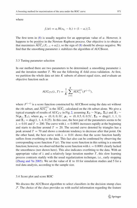
and the iteration number T . We use the following K -fold cross-validation. At first,we partition the whole data set into K subsets of almost equal sizes, and evaluate anobjective function such as

AUCCV(λ, T ) = 1

K

K∑i=1

AUC(i)λ (F (−i)),

where F (−i) is a score function constructed by AUCBoost using the data set without

the i th subset, and AUC(i)λ is the AUCλ calculated on the i th subset alone. We give a

typical example of results of AUCCV in Fig. 2, assuming X0 ∼ N(μ0,�0) and X1 ∼N(μ1,�1), where μ0 = (0, 0, 0, 0)′, μ1 = (0, 0.5, 0, 0.5)′, �0 = diag(1, 1, 1, 1)

and �1 = diag(1, 1, 4, 0.25). In this case, the best pair of the parameters seems to beλ = 0.01 and T = 200. The curve with λ = 0.0001 increases rapidly at the beginningand starts to decline around T = 20. The second curve denoted by triangles has apeak around T = 70 and shows a moderate tendency to decrease after that point. Onthe other hand, the best curve with λ = 0.01 shows that the score function hardlysuffers from overfitting to the data. This fact also can be confirmed by observing thecorresponding score function F(x). The true score function in this setting is a smoothfunction; however, we observed that the score function with λ = 0.0001 clearly lackedthe smoothness (not shown here). This also indicates overfitting to the data. With anappropriate value of λ and a relatively large iteration number T , this slow learningprocess contrasts starkly with the usual regularization technique, i.e., early stopping(Zhang and Yu 2005). We set the value of K to 10 for simulation studies and 5 for areal data analysis, according to the sample size.

3.4 Score plot and score ROC

We discuss the AUCBoost algorithm to select classifiers in the decision stump classF . The choice of the class provides us with useful information regarding the feature

123

972 O. Komori

0 50 100 150 200 250 300

T

0.70

0.72

0.74

0.76

0.78

0.80

AU

CC

V

λ = 0.0001λ = 0.001λ = 0.01λ = 0.1

Fig. 2 Results of AUCCV corresponding to different values of λ, as a function of the number of iterations T

variables in a post-analysis of classification. The final score function F(x) is decom-posed as

F(x) =p∑

k=1

Fk(xk).

The utility of the plot of Fk(xk) against xk (score plot of xk) is referred to by Friedmanet al. (2000) and Kawakita et al. (2005). Observing each score plot very carefully, weare able to not only understand how each feature variable xk influences the classifi-cation performance, but also know which feature variable is the most effective andinformative one. We discuss this utility more in detail in simulation studies. Anotheruseful way to gauge the efficiency of each feature variable is to draw the ROC curve forFk(xk) (score ROC) and calculate the corresponding AUC (score AUC). Fk(xk) rep-resents the contribution of xk to the total classification performance; hence, the valueof the score AUC shows the utility of xk . These measurements are more convenientfor comparing the utilities of feature variables because we can order them accordingto their values.

4 Simulation studies

4.1 Setting

In this section, we present two simulation studies. One is intended to demonstrate thatthe score function F(x) generated by AUCBoost provides a good approximation tothe optimal score function, and that score plots are useful for evaluating each featurevariable’s contribution to F(x). The other is designed to show that, in cases whereseveral outliers exist, AUCBoost is much more powerful and robust than other classi-fication methods such as AdaBoost, GAM and the generalized linear model (GLM).

123


-2 0 2 4x1

42

06

scor

e

42

06

scor

e

42

06

scor

e

42

06

scor

e

-2 0 2x2

-6 -4 -2 0 2 4 6x3

-3 -2 -1 0 1 2 3x4

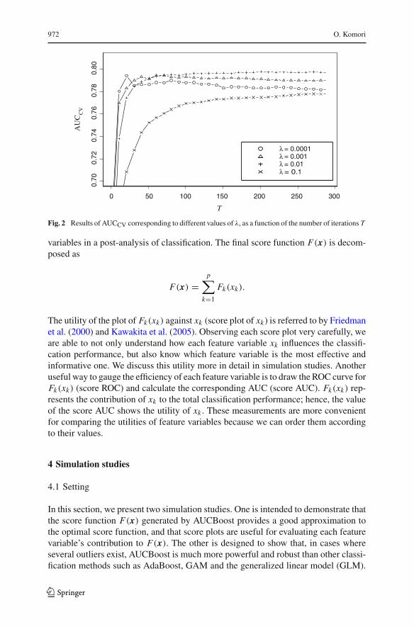
Fig. 3 Score plots for AUCBoost. The black lines indicate mean score plots and the gray lines indicate the95% pointwise confidence bands

The iteration number for AdaBoost is also determined by cross-validation where theobjective function is based on the empirical AUC. Cubic splines are used for GAM,and these simulation studies are done using Splus 8.0. Throughout these simulations,the training sample size is set to be 500 (n0 = 250, n1 = 250) and we evaluated thequality using a test sample of size 200 (n0 = 100 n1 = 100). Summary statistics arebased on 1,000 repetitions.

4.2 Comparison with the optimal score function

Consider the same situation as that of Sect. 3.3: X0 ∼ N(μ0,�0) and X1 ∼ N(μ1,

�1), where μ0 = (0, 0, 0, 0)′, μ1 = (0, 0.5, 0, 0.5)′, �0 = diag(1, 1, 1, 1) and�1 = diag(1, 1, 4, 0.25). From Eq. (4), the optimal score function in this setting isgiven as

FN(x) = x′(�−10 − �−1

1 )x + 2(μ′1�

−11 − μ′

0�−10 )x,

which coincides with a linear score function proposed by Su and Liu (1993) if �0 =�1. The score plots constructed by AUCBoost track FN(x) very well as seen in Fig. 3,where the rug plots at the bottom of each graph depict the data distribution. Clearly, itshows nonlinearity of F(x), especially F3(x3) and F4(x4). From the shape of F3(x3)

we see that x3 with class label 0 has a tendency to concentrate around the origin,compared to x3 with class label 1. On the other hand, in regard to F4(x4), we see theopposite tendency of x4. The flatness of F1(x1) means that x1 is useless for discrim-inating subjects with class 0 from those with class 1, because weak classifiers for x1are rarely chosen, and the weight coefficients are calculated to be very small in theAUCBoost algorithm. Judging from the heights of score plots, x4 seems to be the mostinformative one.

Table 1 shows the results of the score AUCs and the AUCs calculated by AUCBoostand F̂N, where F̂N denotes the estimator of FN. As expected, F̂N achieves superior

123

974 O. Komori

Table 1 The mean score AUCs and the AUCs with 95% confidence bands in parentheses

x1 x2 x3 x4 Total

AUCBoost 0.501 0.628 0.700 0.736 0.828

(0.429, 0.579) (0.548, 0.707) (0.617, 0.774) (0.670, 0.799) (0.772, 0.879)

F̂N 0.500 0.638 0.703 0.742 0.840

(0.425, 0.583) (0.565, 0.714) (0.633, 0.779) (0.668, 0.809) (0.780, 0.887)

performance for all AUCs. It is because F̂N is derived based on the underlying proba-bility distributions; on the other hand, the score function of AUCBoost is constructedby the sample distributions. We also notice that the values of the score AUCs forAUCBoost are in accordance with the heights of the score plots. The utility of x4 isconfirmed again.

4.3 Comparison with other methods

Next, we relax the conditions of the probability distribution a little, and consider amultivariate t-distribution. This is a more practical setting because it contains sev-eral outliers which we often observe in real data. While there are several forms ofmultivariate t-distribution, we use the most common one. The density function ofp-dimensional t-distribution with ν degrees of freedom, mean vector μ and precisionmatrix �−1, is given as

g(x) = (p+ν

2 )√

|�−1| (ν

2 )(νπ)p2

[1 + 1

ν(x − μ)′�−1(x − μ)

]− p+ν2

.

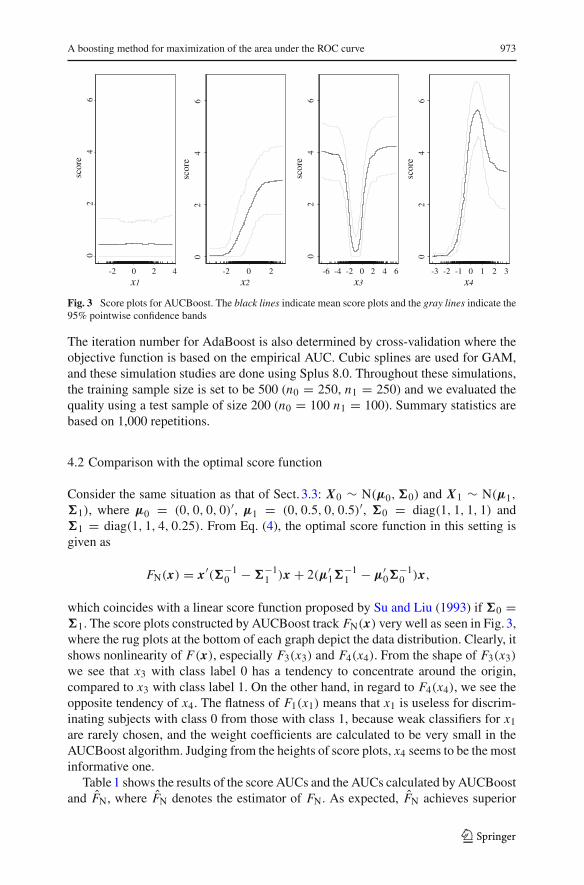
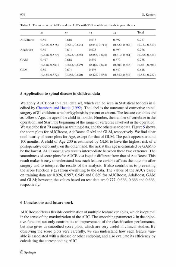
We use the same parameters as those in the previous subsection: μ0 = (0, 0, 0, 0)′,μ1 = (0, 0.5, 0, 0.5)′, �0 = diag(1, 1, 1, 1) and �1 = diag(1, 1, 4, 0.25). To focuson the investigation of the robustness of F(x) constructed by AUCBoost, we consideran extreme situation (ν = 1). Figure 4 shows score plots and score ROCs of x3 forAUCBoost, AdaBoost, GAM and GLM. The range of score plots has been adjusted fora better view. Interestingly, the shape of score plots of AUCBoost and AdaBoost arealmost the same. This is because both of the boosting methods focus only on points thatare useful for the classification. On the other hand, GAM is sensitive to uninformativesamples such as outliers, which causes the GAM’s performance instability (Kawakitaet al. 2005). In regard to GLM, it does not capture the useful information about x3 atall, which is observable from the value of the score AUC (0.496) as well as the shapeof the score ROC. The concavity of the shape of ROC is known to be a necessarycondition of the optimality (Pepe 2003). In the last column of Table 2, we can see thatthe corresponding 95% confidence band of the AUC for AUCBoost is much narrowerthan the others. Among all of them, the result for AUCBoost is the most stable withthe largest mean AUC value (0.787). The smoothing parameter λ contributes to thestable result of AUCBoost.

123


-40

-20

020

40

x3

01234

score

-40

-20

020

40

x3

0.00.20.40.60.8

score

-40

-20

020

40

x3

0.02.0*1013

4.0*1013

6.0*1013

8.0*1013

1.0*1014

score

-40

-20

020

40

x3

01234

score

0.0

0.2

0.4

0.6

0.8

1.0

FPR

0.00.20.40.60.81.0

TPR

0.63

3

0.0

0.2

0.4

0.6

0.8

1.0

FPR

0.00.20.40.60.81.0

TPR

0.62

5

0.0

0.2

0.4

0.6

0.8

1.0

FPR

0.00.20.40.60.81.0

TPR

0.59

9

0.0

0.2

0.4

0.6

0.8

1.0

FPR

0.00.20.40.60.81.0

TPR

0.49

6

Fig

.4R

esul

tsof

scor

epl

ots

(upp

erpa

nels

)an

dsc

ore

RO

Cs

(low

erpa

nels

)fo

rx 3

ofA

UC

Boo

st,A

daB

oost

,GA

Man

dG

LM

.The

blac

kli

nes

indi

cate

mea

nsc

ore

plot

san

dsc

ore

RO

Cs,

and

the

gray

line

sin

dica

teth

e95

%po

intw

ise

confi

denc

eba

nds.

The

confi

denc

eba

ndof

the

scor

epl

otfo

rG

AM

isom

itted

,and

the

min

imum

valu

esof

axes

ofsc

ore

plot

sar

ese

tto

0fo

ra

bette

rvi

ew

123

976 O. Komori

Table 2 The mean score AUCs and the AUCs with 95% confidence bands in parentheses

x1 x2 x3 x4 Total

AUCBoost 0.501 0.616 0.633 0.697 0.787

(0.425, 0.578) (0.541, 0.694) (0.547, 0.711) (0.620, 0.764) (0.723, 0.839)

AdaBoost 0.501 0.601 0.625 0.690 0.776

(0.428, 0.579) (0.522, 0.685) (0.553, 0.696) (0.610, 0.761) (0.705, 0.834)

GAM 0.497 0.618 0.599 0.672 0.738

(0.418, 0.583) (0.543, 0.699) (0.487, 0.694) (0.603, 0.748) (0.661, 0.804)

GLM 0.501 0.601 0.496 0.649 0.648

(0.434, 0.572) (0.388, 0.690) (0.427, 0.555) (0.340, 0.744) (0.533, 0.737)

5 Application to spinal disease in children data

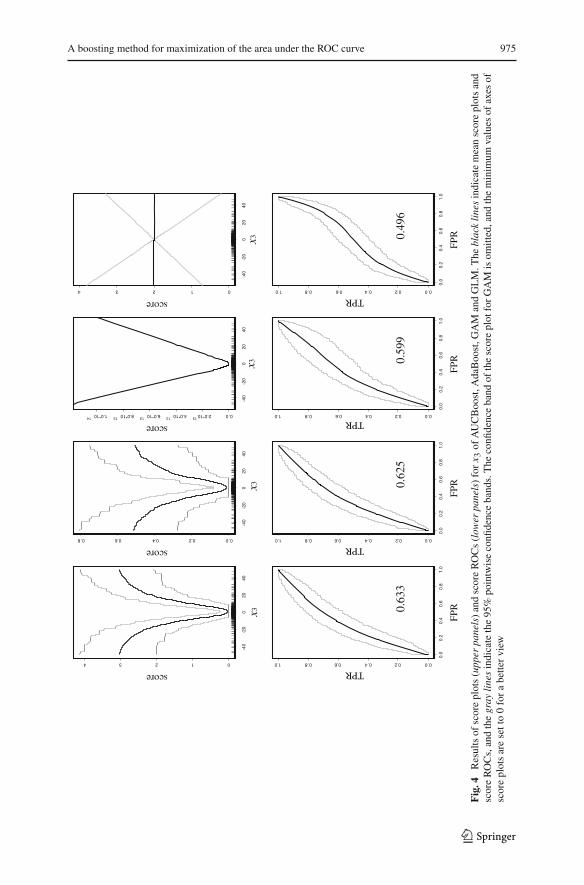
We apply AUCBoost to a real data set, which can be seen in Statistical Models in Sedited by Chambers and Hastie (1992). The label is the outcome of corrective spinalsurgery of 81 children: whether kyphosis is present or absent. The feature variables areas follows: Age, the age of the child in months; Number, the number of vertebrae in theoperation; and Start, the beginning of the range of vertebrae involved in the operation.We used the first 70 samples as training data, and the others as test data. Figure 5 showsthe score plots for AUCBoost, AdaBoost, GAM and GLM, respectively. We find clearnonlinearity of score plots for Age, except for that of GLM. The peak appears around100 months. A child of Age 200 is estimated by GLM to have the highest risk of apostoperative deformity; on the other hand, the risk at this age is estimated by GAM tobe the lowest. AUCBoost gives results intermediate between these two extremes. Thesmoothness of score plots for AUCBoost is quite different from that of AdaBoost. Thisresult makes it easy to understand how each feature variable affects the outcome aftersurgery and to interpret the results of the analysis. It also contributes to preventingthe score function F(x) from overfitting to the data. The values of the AUCs basedon training data are 0.926, 0.997, 0.949 and 0.869 for AUCBoost, AdaBoost, GAMand GLM; however, the values based on test data are 0.777, 0.666, 0.666 and 0.666,respectively.

6 Conclusions and future work

AUCBoost offers a flexible combination of multiple feature variables, which is optimalin the sense of the maximization of the AUC. The smoothing parameter λ in the objec-tive function not only contributes to improvement of the classification performance,but also gives us smoothed score plots, which are very useful in clinical studies. Byobserving the score plots very carefully, we can understand how each feature vari-able is associated with a disease or other endpoint, and also evaluate its efficiency bycalculating the corresponding AUC.

123


0 50 100 150 200

Age

03

21

scor

e

2 4 6 8 10

Number0

32

1sc

ore

5 10 15

Start

03

21

scor

e

20

64

8

scor

e

20

64

8

scor

e

20

64

8

scor

e

scor

e

scor

e

02

46

8

02

46

8

02

46

8

scor

e

0 50 100 150 200

Age

0 50 100 150 200

Age

0 50 100 150 200

Age

21

03

scor

e

2 4 6 8 10

Number

2 4 6 8 10

Number

2 4 6 8 10

Number

21

03

scor

e

5 10 15

Start

5 10 15

Start

5 10 15

Start

21

03

scor

e

Fig. 5 Score plots for AUCBoost, AdaBoost, GAM and GLM from top to bottom. The minimum valuesof each score plot are set to 0 for better view

123

978 O. Komori

From the setting of F which consists of component-based simple classifiers, thescore function of AUCBoost has a similar form to that of GAM. However, there aretwo major differences between them. First, we maximize the AUC instead of thelikelihood. Second, we update the score function by sequentially adding weak clas-sifiers, whereas GAM is based on a backfitting algorithm (Hastie et al. 2001). Theforward stagewise additive modeling gives AUCBoost robustness to distributions ofdata as seen in Sect. 4.3. Thus, AUCBoost is expected to show stable classificationperformance in various situations. This property also makes it easy to take discreteor ordered categorical data into consideration, which is difficult or impossible for thebackfitting algorithm.

A weak point of AUCBoost is that the selection of the tuning parameter λ and Tis time-consuming because we apply a simple cross-validation method. In order toavoid such a computational cost and make it easy to use, a more sophisticated proce-dure is necessary. Recently, Ueki and Fueda (2009) proposed an effective method fordetermining tuning parameters of maximum penalized likelihood estimator. The ideais based on likelihood, not the AUC; however, it could be modified into AUCBoostand help it reduce its computational costs.

AUCBoost can also be applied to a high-dimensional data analysis, in which var-iable selection is much more important than in the low-dimensional data analysis weconsider in this paper. The AUCBoost algorithm implicitly includes a selection pro-cess at each iteration stage, so that informative feature variables are selected as a resultafter applying AUCBoost. This property is similar to GAMBoost (Tutz and Binder2006), which circumvents GAM’s restriction to low-dimensional setting. The conceptof the partial AUC (pAUC) is also of great interest in the analysis of genetic data. Pepeet al. (2003) showed the biological utility of the pAUC for ranking informative genes.We will work on developing partial AUCBoost as one of the appealing extensions ofAUCBoost.

Acknowledgments This study was supported by the Program for Promotion of Fundamental Studies inHealth Sciences of the National Institute of Biomedical Innovation (NIBIO).

References

Bamber, D. (1975). The area above the ordinal dominance graph and the area below the receiver operatingcharacteristic graph. Journal of Mathematical Psychology, 12, 387–415.

Chambers, J. M., Hastie, T. J. (1992). Statistical models in S. Pacific Grove, CA: Wadsworth and Brooks.Eguchi, S., Copas, J. (2002). A class of logistic-type discriminant functions. Biometrika, 89, 1–22.Freund, Y., Schapire, R. E. (1997). A decision-theoretic generalization of on-line learning and an application

to boosting. Journal of Computer and System Sciences, 55, 119–139.Friedman, J., Hastie, T., Tibshirani, R. (2000). Additive logistic regression: A statistical view of boosting

(with discussion). The Annals of Statistics, 28, 337–407.Hastie, T., Tibshirani, R. (1986). Generalized additive models. Statistical Science, 1, 297–318.Hastie, T., Tibshirani, R., Friedman, J. (2001). The elements of statistical learning. New York: Springer.Kawakita, M., Minami, M., Eguchi, S., Lennert-Cody, C. E. (2005). An introduction to the predictive tech-

nique AdaBoost with a comparison to generalized additive models. Fisheries Research, 76, 328–343.Long, P. M., Servedio, R. A. (2007). Boosting the area under the ROC curve. In J. C. Platt, D. Koller, Y.

Singer, S. Roweis (Eds.), Advances in neural information processing systems (Vol. 20, pp. 945–952).Cambridge, MA: MIT Press.

123


Ma, S., Huang, J. (2005). Regularized ROC method for disease classification and biomarker selection withmicroarray data. Bioinformatics, 21, 4356–4362.

Ma, S., Huang, J. (2007). Combining multiple markers for classification using ROC. Biometrics, 63,751–757.

McIntosh, M. W., Pepe, M. S. (2002). Combining several screening tests: Optimality of the risk score.Biometrics, 58, 657–664.

McLachlan, G. J. (2004). Discriminant analysis and statistical pattern recognition. New York: Wiley.Murata, N., Takenouchi, T., Kanamori, T., Eguchi, S. (2004). Information geometry of U -Boost and

Bregman divergence. Neural Computation, 16, 1437–1481.Neyman, J., Pearson, E. S. (1933). On the problem of the most efficient tests of statistical hypotheses.

Philosophical Transactions of the Royal Society of London, Series A, 231, 289–337.Pepe, M. S. (2003). The statistical evaluation of medical tests for classification and prediction. Oxford:

Oxford University Press.Pepe, M. S., Thompson, M. L. (2000). Combining diagnostic test results to increase accuracy. Biostatistics,

1, 123–140.Pepe, M. S., Longton, G., Anderson, G. L., Schummer, M. (2003). Selecting differentially expressed genes

from microarray experiments. Biometrics, 59, 133–142.Pepe, M. S., Cai, T., Longton, G. (2006). Combining predictors for classification using the area under the

receiver operating characteristic curve. Biometrics, 62, 221–229.Pepe, M. S., Janes, H., Longton, G., Leisenring, W., Newcomb, P. (2004). Limitations of the odds ratio in

gauging the performance of a diagnostic, prognostic, or screening marker. American Journal of Epide-miology, 159, 882–890.

Su, J. Q., Liu, J. S. (1993). Linear combinations of multiple diagnostic markers. Journal of the AmericanStatistical Association, 88, 1350–1355.

Takenouchi, T., Eguchi, S. (2004). Robustifying AdaBoost by adding the naive error rate. Neural Compu-tation, 16, 767–787.

Tutz, G., Binder, H. (2006). Generalized additive modeling with implicit variable selection by likelihood-based boosting. Biometrics, 62, 961–971.

Ueki, M., Fueda, K. (2009). Optimal tuning parameter estimation in maximum penalized likelihood method.Annals of the Institute of Statistical Mathematics. doi:10.1007/s10463-008-0186-0.

Wang, Z., Chang, Y. I., Ying, Z., Zhu, L., Yang, Y. (2007). A parsimonious threshold-independent proteinfeature selection method through the are under receiver operating characteristic curve. Bioinformatics,23, 2788–2794.

Zhang, B. T., Yu, B. (2005). Boosting with early stopping: Convergence and consistency. The Annals ofStatistics, 33, 1538–1579.

Zhou, X. H., Obuchowski, N. A., McClish, D. K. (2002). Statistical methods in diagnostic medicine. NewYork: Wiley.

123

http://dx.doi.org/10.1007/s10463-008-0186-0

Documents

A boosting method for maximization of the area under the ROC curve