Embed Size (px)
Citation preview
Bettina Plomp
MSc Industrial Engineering & Management
Production & Logistics Management
Enschede, 08-10-2019
A BOTTLENECK ANALYSIS TO INCREASE THROUGHPUT AT APOLLO VREDESTEIN B.V.

Page | ii
Page | iii
Document Title A bottleneck analysis to increase throughput at Apollo Vredestein B.V.
Date 08-10-2019
Author B.I. Plomp
Master Program Industrial Engineering and Management
Specialization: Production and Logistics Management
Graduation Committee University of Twente Dr. E. Topan
Faculty of Behavioral Management and Social Sciences Dr.Ir. J.M.J. Schutten
Faculty of Behavioral Management and Social Sciences
Apollo Vredestein B.V. T. Van der Linden

Page | iv

Page | v
Acknowledgements This thesis concludes my Master in Industrial Engineering and Management (specialization
Production and Logistics Management) at the University of Twente. In the past eight months I have
performed a bottleneck analysis at Apollo Vredestein B.V., which has been an exciting and interesting
assignment. From my first day at Vredestein I have felt welcome and I would like to thank my
colleagues for their kindness and willingness to help.
First of all, I would like to thank Tamara van der Linden for her guidance, feedback and fun times at
the office. She has been very committed and always willing to discuss my thesis. Furthermore, I
would like to thank my direct colleagues at the industrial engineering department for helpful
discussions and information and all the employees of Vredestein who have helped me in any way for
their collaboration within the research and acceptance of me joining (some of) their meetings.
From the University of Twente I would like to thank my supervisors, Engin Topan and Marco
Schutten. With their feedback and discussions, they have challenged me and helped me improve my
thesis.
Last, yet not least important, I would like to thank my family and friends. I highly appreciate their
interest and support and I know I can always count on them.
Bettina Plomp
Enschede, October 2019

Page | vi
Page | vii
Management summary We perform this research at Apollo Vredestein B.V as a Master thesis for the study Industrial
Engineering & Management and specialization Production and Logistics Management. The tyres of
Apollo Vredestein have become more diverse and this has increased the complexity within the
production site. Not all processes are adapted to this change, which has increased the production
costs per tyre. To be able to compete, it is crucial for Apollo Vredestein to improve their efficiency
and with that lower the costs per tyre. To achieve both lower costs per tyre and a higher throughput,
we decide to improve performance by following the concept called Theory of Constraints. Therefore,
we define the main research question as follows:
“How can Apollo Vredestein identify the most significant bottleneck machine within the production
line of agricultural and space master tyres, improve the most significant bottleneck machine, and
align non-bottleneck machines to increase the throughput of the system?”
Bottleneck identification
We limit this research to the production line of agricultural and space master tyres. To set up the
bottleneck identification process, we take the requirements of Apollo Vredestein and the
characteristics of the bottleneck identification methods known in literature into account. We set up a
bottleneck identification process that consists of four phases. The first phase filters on data
availability to identify non-bottlenecks. The second phase performs the turning point method and
the third phase performs the utilization method to identify the bottleneck. Finally, the fourth phase
gives a conclusion on the location of the bottleneck and validates the result. After executing the
bottleneck identification process, we conclude that the current bottleneck is a machine called the
ART. The ART is a bead-making machine that produces beads for both agricultural and space master
tyres.
Bottleneck improvement
We perform a root cause analysis to define a focus of improvement at the bottleneck machine. We
formulate the problem as “limited throughput at the ART”. We use an Ishikawa diagram to present
an overview of the potential causes and we arrange them in a Probability-Impact Matrix. Using this
matrix, we decide that improving the cause “fine-tuning of the machine” is of the highest
importance. To decrease the amount of time that is spent on fine-tuning of the machine, Apollo
Vredestein should limit the possibilities to fine-tune. First, by creating an agreed upon setting or
settings. Second, by making some settings that do not have to be accessible non-accessible for
operators. Because this solution requires a very thorough understanding of the machine and the
effects of certain components, we recommend the process technologist to improve this cause.
Furthermore, we conclude from the Probability-Impact matrix to focus on a second cause. We focus
on the cause “no wrapping material” and specifically on the two sub-causes “the length of a roll is
not measured and not booked” and “the current buffer for wrapping material is not sufficient”.
Improving these sub-causes contributes to subordinating or aligning the non-bottleneck processes.
Subordinate non-bottleneck processes
Apollo Vredestein can reduce the shortage of wrapping material by improving the accuracy of the
inventory of wrapping material and by implementing an inventory control policy to buffer against
uncertainties. We set up a measurement method to estimate the length of a roll from the diameter
of a roll and use this method to generate data on the length of a roll of wrapping material. We
Page | viii
analyze the data and decide whether we should change the current approach of booking 250 meters
per roll. There are two options to improve the accuracy of the inventory. The first option is adjusting
the amount of meters booked per roll of wrapping material from 250 to 216 meters. This solution
improves the accuracy with the least effort but does not offer a precise representation of the
inventory. This option can be expanded by manually measuring small rolls that are outliers. After the
operator measures the diameter, he or she can manually enter the diameter in PIBS (the production
information and control system used within Vredestein) and PIBS estimates the corresponding
length. This option requires a little bit of time from the operators, because measuring the diameter is
only required for a very small amount of rolls. The second option is to measure the length of a roll in
each batch. This can be done by manually measuring the diameter of the roll, entering the diameter
in PIBS and with that estimating the corresponding length. Because one roll of each batch needs to
be measured, this option requires more time from the operator. It can also be done by adding
measuring equipment at the machine where wrapping material is produced, the ORION. Then, it
does not require time from the operator, but it does require an initial investment for the measuring
equipment.
We also compare some inventory control policies and set up an inventory control policy for Apollo
Vredestein to reduce the shortage of wrapping material. We decide a (R,s,Q) policy goes best with
the situation at Apollo Vredestein, because it has a periodic review period, a fixed order quantity and
the possibility to order a multiple of Q. Using this policy, every R units of time the inventory position
is reviewed. If the inventory position is at or below the reorder point s, an integral multiple of a fixed
quantity Q is used, such that the inventory position is raised to a value between s and s + Q. If the
inventory position is above s, no order is placed until the next review moment. Internal supply
uncertainty caused by queue waiting time and internal demand uncertainty caused by scrap are the
two major types of uncertainty taken into account for determining the parameters. There are two
stock keeping units (SKUs) of wrapping material: HE01-00-0034 and HE01-00-0038. For SKU HE01-00-
0034 the policy has a review period R of one shift, order quantity Q of 40 rolls and safety stock SS of 1
roll. For SKU HE01-00-0038 the policy has a review period R of one shift, order quantity Q of 81 rolls
and safety stock SS of 2 rolls. Given that the amount of meters booked per roll of wrapping material
is updated to 216 meters, these parameters result in a weighted average fill rate 𝑃2 of 0.9997. This
equals a yearly shortage of 597.7 meters or 82 minutes.
Recommendations
We recommend reducing the amount of shortage of wrapping material by implementing the option
to adjust the amount of meters booked per roll of wrapping material from 250 to 216 meters. We
recommend expanding this option with manually measuring and booking small rolls that are outliers.
If the shortage of wrapping material has improved sufficiently (by assessment of Apollo Vredestein),
we recommend maintaining this solution. If it has not improved sufficiently, we recommend to start
measuring and booking the length of each roll. Depending on the preference of Apollo Vredestein
this can be done by manually measuring or automatically measuring with (to be installed) measuring
equipment. We recommend to further reduce the amount of shortage of wrapping material by
implementing the (R,s,Q) policy. Also, we recommend Apollo Vredestein to continue to identify the
bottleneck in the future. This can be once a month or once every few months. If the ART remains the
bottleneck after implementing the recommendations described so far, we recommend decreasing
the amount of time that is spent on fine-tuning the machine and, if necessary, some other causes
identified in the root cause analysis.

Page | ix
Abbreviations AGRI AGRIcultural
BPR Business Process Re-engineering C Storage capacity IE Industrial Engineering KPI Key Performance Indicator LM Lean Management MHE Material Handling Equipment NGT No GreenTyre PCT Passenger Car Tyres PIBS Productie Informatie en BesturingsSysteem. Translates to: Production
Information and Control System PIPO Periodieke Inspectie Preventief Onderhoud. Translates to: Periodic Inspection
Preventive Maintenance Q Order quantity R Review interval/period RM Replacement Market S Order-up-to level s Reorder point SiS Six Sigma SKU Stock Keeping Unit SM Space Master SS Safety Stock TB Blockage times TBM Tyre Building Machine TOC Theory Of Constraints TQM Total Quality Management TS Starvation times WIP Work In Process

Page | x
Page | xi
Content
Acknowledgements .................................................................................................................................. v
Management summary .......................................................................................................................... vii
Abbreviations .......................................................................................................................................... ix
1. Introduction ..................................................................................................................................... 1
1.1 About Apollo Vredestein ......................................................................................................... 1
1.2 Research motivation ................................................................................................................ 2
1.3 Bottleneck................................................................................................................................ 3
1.4 Theory of Constraints .............................................................................................................. 4
1.5 Research objective .................................................................................................................. 5
1.6 Organizational structure .......................................................................................................... 6
1.7 Root cause analysis.................................................................................................................. 6
1.8 Research scope ........................................................................................................................ 8
1.9 Research questions.................................................................................................................. 9
2. Current situation ........................................................................................................................... 11
2.1 Tyre structure ........................................................................................................................ 11
2.2 Production process ................................................................................................................ 12
2.3 Product flow .......................................................................................................................... 14
2.4 Production planning .............................................................................................................. 16
2.5 Intermediate stock ................................................................................................................ 17
2.6 System performance ............................................................................................................. 18
2.7 Wrapping material ................................................................................................................. 19
2.8 Conclusion ............................................................................................................................. 20
3. Literature review ........................................................................................................................... 23
3.1 Operations management philosophies ................................................................................. 23
3.2 Bottleneck identification methods ........................................................................................ 24
3.3 Inventory control ................................................................................................................... 28
3.3 Conclusion ............................................................................................................................. 37
4. Model framework .......................................................................................................................... 39
4.1 Model framework flowchart ................................................................................................. 39
4.2 Bottleneck identification process .......................................................................................... 40
4.3 Bottleneck optimization process ........................................................................................... 44
4.4 Process to subordinate all non-bottleneck processes ........................................................... 45
4.5 Conclusion ............................................................................................................................. 49
Page | xii
5. Model implementation ................................................................................................................. 51
5.1 Bottleneck identification ....................................................................................................... 51
5.2 Bottleneck optimization ........................................................................................................ 55
5.3 Subordinate non-bottleneck processes................................................................................. 60
5.4 Conclusion ............................................................................................................................. 68
6. Conclusion, recommendations and discussion ............................................................................. 69
6.1 Conclusion ............................................................................................................................. 69
6.2 Recommendations................................................................................................................. 70
6.3 Discussion .............................................................................................................................. 72
References ............................................................................................................................................. 73
Appendix ................................................................................................................................................ 77
Appendix 1: Flowcharts with distinction between components ....................................................... 77
Appendix 2: Dashboard to identify the bottleneck ........................................................................... 79
Appendix 3: Extensive descriptions of causes ................................................................................... 85
Appendix 4A: Probability-Impact Matrix Form ................................................................................. 88
Appendix 4B: Average Probability-Impact Matrix ............................................................................. 90
Appendix 5: Template for rolls of wrapping material ....................................................................... 91
Page | 1
1. Introduction This chapter describes the research approach. First, in Section 1.1 we introduce the company where
the research takes place. Section 1.2 gives the motivation for the research. Next, Section 1.3
elaborates on the definition of the bottleneck. Section 1.4 introduces the management concept
called Theory of Constrains. We formulate the research objective in Section 1.5. Section 1.6 gives
information about the organizational structure and Section 1.7 contains a root cause analysis. Section
1.8 gives the scope of the research. Finally, Section 1.9 presents the research questions.
1.1 About Apollo Vredestein Vredestein is established in the Netherlands in 1909 and has a rich heritage in the world of car tyres.
With a legacy of over 100 years, the Vredestein brand has achieved premium brand status in the
automotive industry. Today, Apollo Vredestein B.V. is part of Apollo Tyres Ltd from India. Apollo
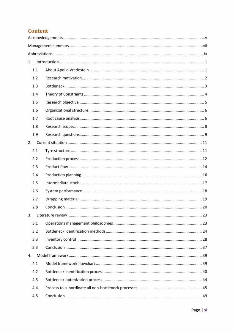
Tyres is a multinational with offices all around the world. Figure 1.1 shows a map with all the Apollo
offices and plants around the world. Apollo Vredestein manufactures and sells high quality tyres and
their tyres have won multiple awards. They sell for both brands Apollo and Vredestein in Europe.
Beyond Europe the tyres are available in over 100 countries across the globe. The head office of
Apollo Vredestein is in Amsterdam and the manufacturing sites are in Enschede and Gyöngyöshalász
(Hungary).
Figure 1.1: World map with all Apollo offices and plants. Reprinted from “corporate-
presentation2017”, by Apollo Vredestein B.V., 2017.
The company delivers two types of markets, Original Equipment Manufacturers and Replacement
Market. Original Equipment (OE) tyres are supplied directly to the vehicle manufacturers that
assemble vehicles in their assembly plant. Thus, these tyres are used in new cars that are yet to be
sold. The Replacement Market (RM), also called aftermarket, supplies accessories, spare parts,
second-hand equipment, and other goods and services used in repair and maintenance. Apollo
Vredestein supplies tyres to the RM that can be used for instance if a tyre is worn out. Within these
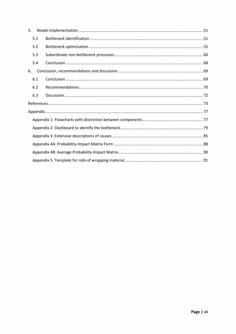
two markets they deliver to three sectors: Passenger Car Tyres (PCT), Space Master Tyres (SM) and
Page | 2
Agricultural Tyres (AGRI). Figure 1.2, Figure 1.3, and Figure 1.4 respectively represent the three tyre
sectors.
Figure 1.2: PCT tyres.
Figure 1.3: SM tyres.
Figure 1.4: AGRI tyres.
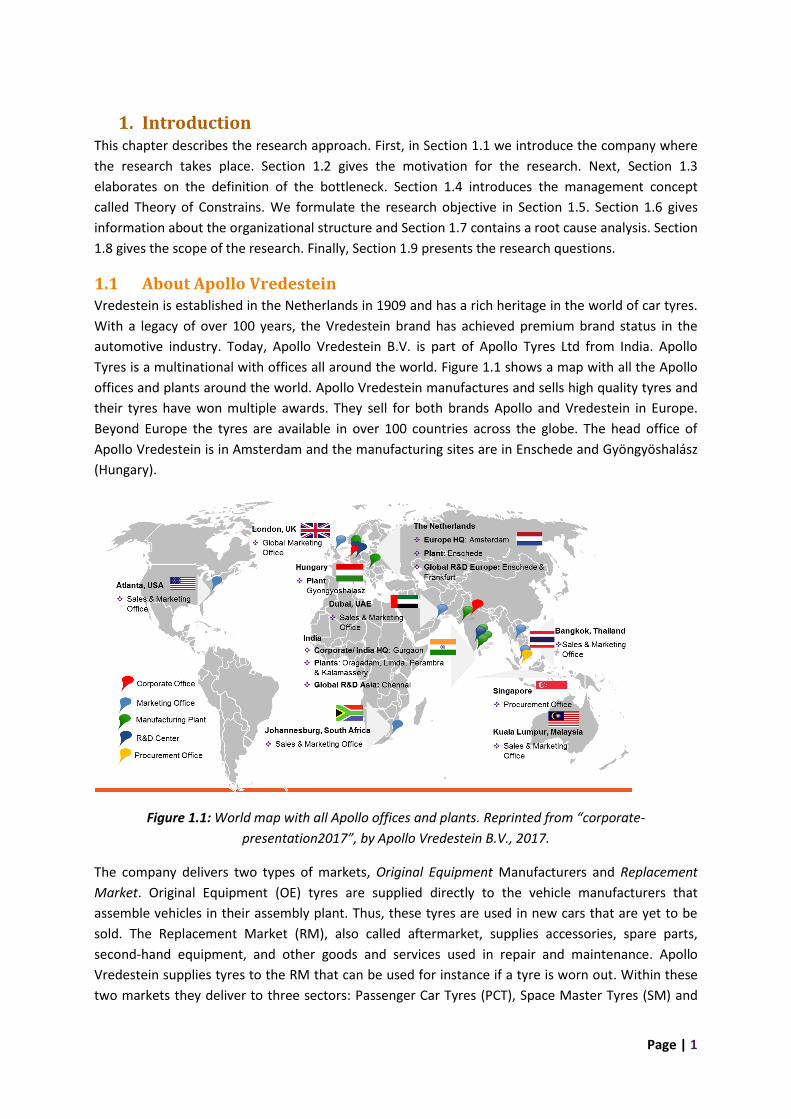
Their tyres are very diverse, also within the tyre sector. There are many different sizes, profiles and specifications that lead to a large amount of stock keeping units (SKUs). Most are obvious differences such as the size, profiles, or purpose (for instance summer/winter). Figure 1.5 shows an example. The tyres on the left and right are both AGRI tyres, but they have a different size and profile and thus look very different. However, sometimes the tyre diversity is not even visible for the eye. Figure 1.6 and Figure 1.7 present an example: the tyres have the exact same size and profile, but a different load index. The load index refers to the maximum weight that a tire can support when properly inflated. A higher load index means that the tyre can support a higher weight. The tyres have different layers of ply, layers of breaker and a different strength of the bead to achieve a specific load index. Thus, these are two tyres with different specifications and a different construction, but they have the same appearance. This is an example for AGRI tyres, but the same sort of examples can be found for PCT and SM tyres.
Figure 1.5: Visible tyre
differences.
Figure 1.6: AGRI tyre
540/65R30 (143 D).
Figure 1.7: AGRI tyre
540/65R30 (150 D).
1.2 Research motivation The tyres of Apollo Vredestein have become more diverse and this has increased the complexity
within the production site. Not all processes are adapted to this change, which has increased the
production costs per tyre. To be able to compete, it is crucial for Apollo Vredestein to improve their
efficiency and with that lower the costs per tyre. Also, in the current situation the production
Page | 3
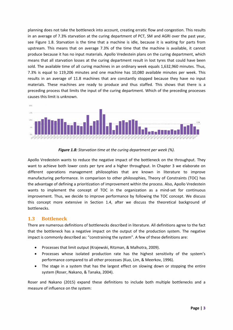
planning does not take the bottleneck into account, creating erratic flow and congestion. This results
in an average of 7.3% starvation at the curing department of PCT, SM and AGRI over the past year,
see Figure 1.8. Starvation is the time that a machine is idle, because it is waiting for parts from
upstream. This means that on average 7.3% of the time that the machine is available, it cannot
produce because it has no input materials. Apollo Vredestein plans on the curing department, which
means that all starvation losses at the curing department result in lost tyres that could have been
sold. The available time of all curing machines in an ordinary week equals 1,632,960 minutes. Thus,
7.3% is equal to 119,206 minutes and one machine has 10,080 available minutes per week. This
results in an average of 11.8 machines that are constantly stopped because they have no input
materials. These machines are ready to produce and thus staffed. This shows that there is a
preceding process that limits the input of the curing department. Which of the preceding processes
causes this limit is unknown.
Figure 1.8: Starvation time at the curing department per week (%).
Apollo Vredestein wants to reduce the negative impact of the bottleneck on the throughput. They
want to achieve both lower costs per tyre and a higher throughput. In Chapter 3 we elaborate on
different operations management philosophies that are known in literature to improve
manufacturing performance. In comparison to other philosophies, Theory of Constraints (TOC) has
the advantage of defining a prioritization of improvement within the process. Also, Apollo Vredestein
wants to implement the concept of TOC in the organization as a mind-set for continuous
improvement. Thus, we decide to improve performance by following the TOC concept. We discuss
this concept more extensive in Section 1.4, after we discuss the theoretical background of
bottlenecks.
1.3 Bottleneck There are numerous definitions of bottlenecks described in literature. All definitions agree to the fact
that the bottleneck has a negative impact on the output of the production system. The negative
impact is commonly described as: “constraining the system”. A few of these definitions are:
• Processes that limit output (Krajewski, Ritzman, & Malhotra, 2009).
• Processes whose isolated production rate has the highest sensitivity of the system’s
performance compared to all other processes (Kuo, Lim, & Meerkov, 1996).
• The stage in a system that has the largest effect on slowing down or stopping the entire
system (Roser, Nakano, & Tanaka, 2004).
Roser and Nakano (2015) expand these definitions to include both multiple bottlenecks and a
measure of influence on the system:
Page | 4
“Bottlenecks are processes that influence the throughput of the entire system. The larger the
influence, the more significant is the bottleneck.” (Roser & Nakano, 2015)
Bottlenecks in dynamic systems are not stable as they can shift due to machine downtime such as
faults or preventive maintenance. A shifting bottleneck means that the location of the bottleneck
changes over time. The more balanced the system, the more the capacity of all parts within the
system is the same. This increases the influence of temporary downtime on the location of the
bottleneck. Thus, the more balanced the system, the more probable it is that the bottleneck will
shift. These shifting bottlenecks are the system’s constraint for only a certain period of time, so they
are momentary bottlenecks. It can occur that the high level of balance within a system results in a
different bottleneck every minute. This is called a continuously shifting bottleneck.
There are two types of bottlenecks. Short-term bottlenecks, also called momentary bottlenecks, are
caused by temporary problems. For instance, an employee who becomes ill and the work cannot be
done by someone else. This causes a backlog of work until the person is back. Or, an accident at a
machine can lead to an unplanned stop. This also causes a backlog of work until the situation is
resolved and the machine is turned back on. Long-term bottlenecks are blockages that occur
regularly. For instance, general inefficiency of a machine. Both short-term and long-term bottlenecks
can shift over time, which results in multiple bottlenecks. Each bottleneck has a certain amount of
influence on the throughput of the entire system. The bottleneck with the largest influence is the
most significant bottleneck.
Furthermore, bottlenecks can be internal or external to the system (Cox III & Schleier, 2010). An
internal bottleneck occurs when the market demands more from the system than it can deliver. If
this is the case, we deal with an operational bottleneck and the focus of the organization should be
on identifying and improving the bottleneck within the system. An external bottleneck exists when
the system can produce more but cannot sell it. This can be a market constraint or a sales process
constraint. If this is the case, then the focus should be on creating more demand.
In complex and dynamic systems, it is expected that there are multiple bottlenecks. We cannot look
at all the bottlenecks at once, thus we start with analyzing the most significant one. The bottlenecks
can move over time, because of improvements, changes in demand, etc. If there is a new most
significant bottleneck, we want to determine the location of that bottleneck. Thus, we want to be
able to continuously monitor and identify the bottlenecks. Section 1.4 elaborates on Theory of
Constraints: a concept that continuously analyzes the bottleneck. The identification of the bottleneck
is a part of this concept.
1.4 Theory of Constraints In the seventies, Eliyahu Goldratt criticized the operations management methods that were used in
that time and work as if it were true that “optimizing each part of the system causes the system as a
whole be optimized”. Goldratt developed a new method, called Theory of Constraints (TOC). Goldratt
and Cox convey the concepts of TOC in the book The goal (Goldratt & Cox, 1986). This management
concept recognizes that there are limitations to the performance of a system caused by a very small
number of elements in the system. TOC emphasizes a five steps process of ongoing improvement,
see Figure 1.9.

Page | 5
• STEP 1: Identify the system’s constraint(s), also called bottlenecks. Constraints may be
physical (e.g. materials, machines, people, demand level) or managerial.
• STEP 2: Exploit the constraint(s). We decide how to optimize the system’s constraint(s). The
goal is to achieve the highest throughput possible at the constraint(s) with the system’s
resources.
• STEP 3: Subordinate everything else to the above decision, i.e. adjust the other processes to
support the constraint(s). Because constraints determine a firm’s throughput, having the
right resources at the right time at the constraint is vital. Thus, every other process in the
system (i.e. non-constraints) must be adjusted to support the maximum effectiveness of the
constraint. If the effectiveness of the constraint increases, so does the effectiveness of the
system. Any resource produced that is not needed will not improve throughput but will
increase unnecessary inventory. Thus, the other processes should support the constraint, but
should not overproduce.
• STEP 4: Elevate the constraint(s), i.e. improve the system’s constraint(s). If the existing
constraints are still the most critical in the system, capacity can be added. Eventually, the
constraint is broken and the system will encounter a new constraint.
• STEP 5: Prevent inertia. If in any of the previous steps a constraint is broken, go back to Step
1.
Figure 1.9: Flowchart of the five steps of ongoing improvement.
Operational performance measures defined by TOC are throughput, inventory and operating
expense. According to TOC, throughput is the rate at which the system generates money through
sales. Thus, output that is not sold is not throughput but inventory. Inventory is all money invested in
things the system intends to sell. Finally, operating expense is the money spent turning inventory
into throughput. This includes expenditures such as direct and indirect labor, supplies and outside
contractors.
The steps of ongoing improvement facilitate the successful execution of a TOC implementation.
Therefore, we use these steps as a guideline for this research.
1.5 Research objective Project objective: Create a dashboard to support the first step of the TOC cycle: identify the
bottleneck. Also, find the causes of the most significant bottleneck for the current situation and
create a solution accordingly to increase the throughput. Finally, align other processes to support the
bottleneck.
Remarks:

Page | 6
1. This project is part of a bigger project where the goal is to increase the throughput (the
number of tyres produced according to sales plan), while lowering operational expenses and
inventory for both PCT as SM & AGRI by following the concept of TOC.
2. The research objective includes step 1 to 3 of the TOC cycle of ongoing improvement. The
dashboard is a tool that can be used when this cycle is repeated in the future. The dashboard
will aid Apollo Vredestein to perform step 1 “Identify the system’s constraint(s)” of the TOC
cycle of ongoing improvement. Thus, the dashboard will help identify the bottleneck using
the data. Step 2 to 5 cannot be performed using only data and the knowledge of the
performer. Therefore, Apollo Vredestein will have to independently perform these steps in
the future.
1.6 Organizational structure Figure 1.10 represents the production at Apollo Vredestein which consists of roughly five stages.
These stages can differ slightly per sector, as explained below. The first stage is mixing where a
rubber compound is formed by mixing rubber and a certain combination of chemicals. Next, the
rubber is processed at the second stage, semi-finished products. In this stage the rubber is processed
into components by means of extrusion, calendaring and cutting. The third stage, assembly, collects
the components needed and starts building the tyre. The assembled tyre is called a greentyre. The
greentyre moves to the fourth stage, curing. Here, the greentyre is vulcanized, or cured, by applying
heat and pressure in special machines to produce the finished tyre. The last stage differs per sector
and can be uniformity, mounting or both. For PCT, the last stage is limited to uniformity and includes
the inspection of the final product. For SM, the last stage is limited to mounting and includes putting
the tyres onto the wheels. AGRI can have none, one or both of these steps. If requested by the
manufacturer, OE tyres (AGRI) can go to uniformity. Also, some of the tyre types (AGRI) go to
mounting. Section 2.2 gives a more detailed description of the production process. To manage the
five stages, also called departments, Vredestein has six business teams and there are some additional
teams to support the production, such as Industrial Engineering, Product Industrialization, Plant
Engineering, and Quality Assurance & IT.
Figure 1.10: The five stages that roughly form the production.
PCT largely has its own production process and is limited by the demand from the market. This
means that the bottleneck is external, i.e. the market. AGRI and SM share more machines and are
both limited by the production capacity, i.e. the bottleneck is internal. As PCT and AGRI/SM share
less machines, we treat PCT as a separate production process.
1.7 Root cause analysis To get an understanding of the problem and its causes, we perform a root cause analysis in which we
create a problem tree for the main problem: limited throughput of the system. Figure 1.11
represents the problem tree. Limited throughput can be caused by an internal or external bottleneck
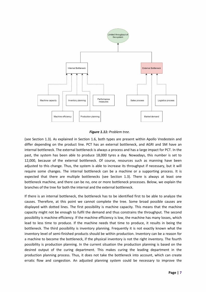
Page | 7
(see Section 1.3). As explained in Section 1.6, both types are present within Apollo Vredestein and
differ depending on the product line. PCT has an external bottleneck, and AGRI and SM have an
internal bottleneck. The external bottleneck is always a process and has a large impact for PCT. In the
past, the system has been able to produce 18,000 tyres a day. Nowadays, this number is set to
12,000, because of the external bottleneck. Of course, resources such as manning have been
adjusted to this change. Thus, the system is able to increase its throughput if necessary, but it will
require some changes. The internal bottleneck can be a machine or a supporting process. It is
expected that there are multiple bottlenecks (see Section 1.3). There is always at least one
bottleneck machine, and there can be no, one or more bottleneck processes. Below, we explain the
branches of the tree for both the internal and the external bottleneck.
If there is an internal bottleneck, the bottleneck has to be identified first to be able to analyze the
causes. Therefore, at this point we cannot complete the tree. Some broad possible causes are
displayed with dotted lines. The first possibility is machine capacity. This means that the machine
capacity might not be enough to fulfil the demand and thus constrains the throughput. The second
possibility is machine efficiency. If the machine efficiency is low, the machine has many losses, which
lead to less time to produce. If the machine needs that time to produce, it results in being the
bottleneck. The third possibility is inventory planning. Frequently it is not exactly known what the
inventory level of semi-finished products should be within production. Inventory can be a reason for
a machine to become the bottleneck, if the physical inventory is not the right inventory. The fourth
possibility is production planning. In the current situation the production planning is based on the
desired output of the curing department. This makes curing the leading department in the
production planning process. Thus, it does not take the bottleneck into account, which can create
erratic flow and congestion. An adjusted planning system could be necessary to improve the
Figure 1.11: Problem tree.

Page | 8
performance of the bottleneck machine. Finally, the fifth possibility is performance measures. The
current key performance indicators (KPIs) for each sub process lead to local efficiencies. In order to
stimulate behavior to create an efficient overall process, new KPIs could be necessary that stimulate
global efficiencies. Also, the current local KPIs are not supporting the production planning. Because
of this, the production planning is regularly not followed correctly. This means that (without
consulting a planner) either too many or too few units are produced in comparison to the production
planning. This can lead to losses at the bottleneck machine.
An external bottleneck can have multiple causes. Figure 1.11 displays some broad possible causes
with dotted lines. An external bottleneck is always outside of the plant, i.e. the production area. The
production area includes all processes that directly influence the production. Thus, the production
area includes for instance the machines, machine schedules, and intermediate stock levels. The
production area excludes all processes that determine what part of produced products is sold. Thus,
the production area excludes for instance demand forecasting, sales and logistics outside the plant.
These processes are included at the headquarter. We conduct this research at the plant. This
concludes that an external bottleneck is not something the plant can control and following the
methodology of Heerkens & van Winden (20012) we do not consider this the core problem.
1.8 Research scope This research focuses on increasing the throughput by implementing the TOC concept. We should
focus on the core problem (Heerkens & van Winden, 2012), therefore the external bottleneck is out
of scope, see Section 1.7. Thus, we choose to focus on the bottleneck within production, the internal
bottleneck. The core problem of the internal bottleneck can be defined after the bottleneck is
identified. Focusing on the internal bottleneck means that we look only at the production process for
AGRI and SM. While identifying the most significant bottleneck we focus on the most significant
bottleneck machine and leave out the bottleneck processes, because of the following. There is at
least one bottleneck machine. It does not necessarily have to be the most significant bottleneck,
because a bottleneck process can be the most significant bottleneck. However, if there is a
bottleneck process, it is most likely also influencing the throughput of the bottleneck machine. This
means that a bottleneck process becomes visible during the analysis of the bottleneck machine as a
cause of limited throughput at the bottleneck machine. If the influence of the bottleneck process is
big, the problem will be dealt with in step 2 of the TOC cycle. This decision increases the reusability
and the feasibility of a dashboard supporting the identification phase, while taking all internal
bottlenecks into account. Thus, we focus on identifying the most significant bottleneck machine.
Also, the last stage of production called uniformity & mounting is left out of the scope. This is the last
production step that is executed outside of the plant, for both AGRI and SM. Also, it is known that
Vredestein cannot meet the demand at the curing department, see Section 1.2. Thus, there is a
limiting process in the preceding processes of the curing department. Because the last stage is
executed outside the plant and we know there is a bottleneck within the plant, we leave it out of the
scope.
As explained in Section 1.3, we expect multiple bottlenecks in complex and dynamic systems. We
cannot look at all the bottlenecks at once, thus within this research we focus on the most significant
bottleneck and exclude other bottlenecks.
Page | 9
To reach the project objective, we go through steps one to three of the cycle of ongoing
improvement. Apollo Vredestein wants to explore the options of improvement without big
investments. Also, due to the time limit we do not repeat the cycle. Therefore, steps four and five are
out of scope.
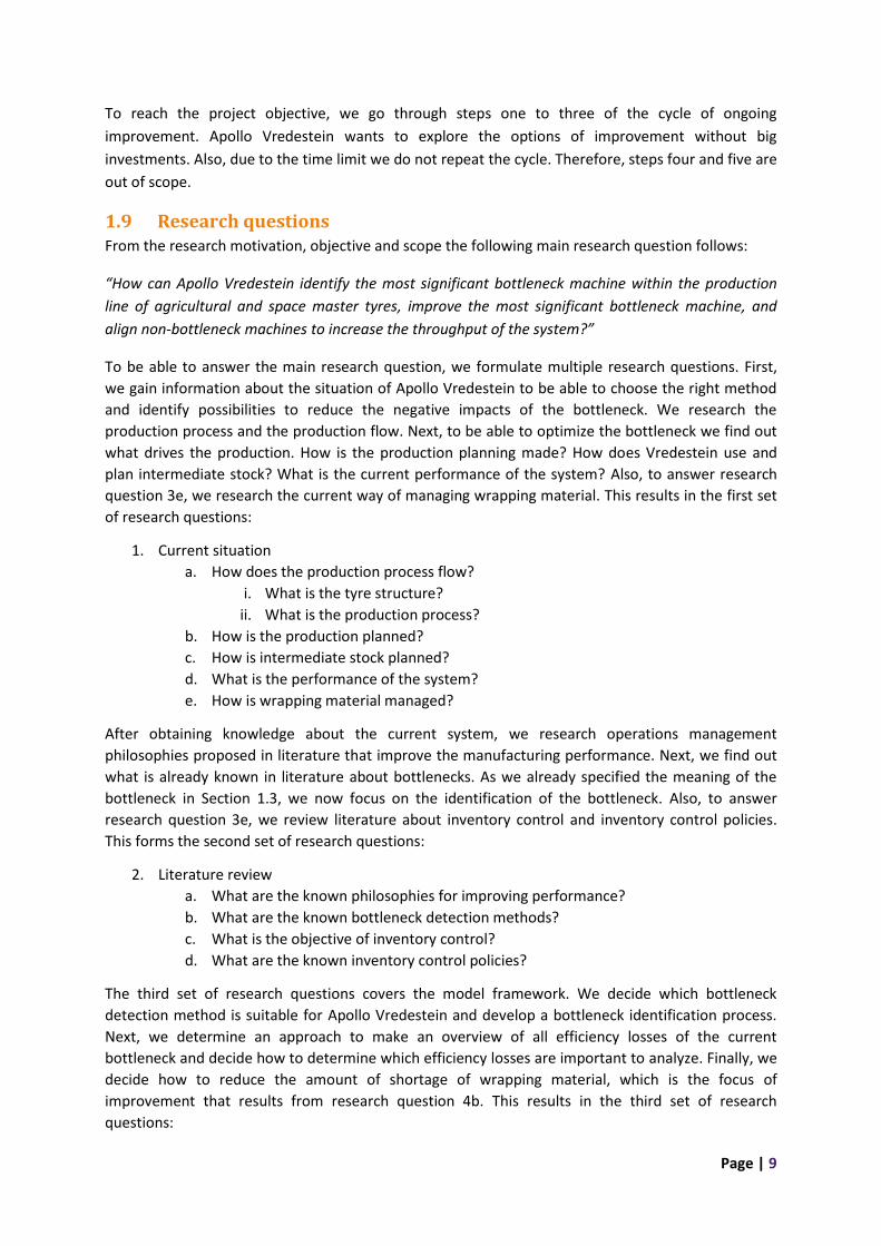
1.9 Research questions From the research motivation, objective and scope the following main research question follows:
“How can Apollo Vredestein identify the most significant bottleneck machine within the production
line of agricultural and space master tyres, improve the most significant bottleneck machine, and
align non-bottleneck machines to increase the throughput of the system?”
To be able to answer the main research question, we formulate multiple research questions. First,
we gain information about the situation of Apollo Vredestein to be able to choose the right method
and identify possibilities to reduce the negative impacts of the bottleneck. We research the
production process and the production flow. Next, to be able to optimize the bottleneck we find out
what drives the production. How is the production planning made? How does Vredestein use and
plan intermediate stock? What is the current performance of the system? Also, to answer research
question 3e, we research the current way of managing wrapping material. This results in the first set
of research questions:
1. Current situation
a. How does the production process flow?
i. What is the tyre structure?
ii. What is the production process?
b. How is the production planned?
c. How is intermediate stock planned?
d. What is the performance of the system?
e. How is wrapping material managed?
After obtaining knowledge about the current system, we research operations management
philosophies proposed in literature that improve the manufacturing performance. Next, we find out
what is already known in literature about bottlenecks. As we already specified the meaning of the
bottleneck in Section 1.3, we now focus on the identification of the bottleneck. Also, to answer
research question 3e, we review literature about inventory control and inventory control policies.
This forms the second set of research questions:
2. Literature review
a. What are the known philosophies for improving performance?
b. What are the known bottleneck detection methods?
c. What is the objective of inventory control?
d. What are the known inventory control policies?
The third set of research questions covers the model framework. We decide which bottleneck
detection method is suitable for Apollo Vredestein and develop a bottleneck identification process.
Next, we determine an approach to make an overview of all efficiency losses of the current
bottleneck and decide how to determine which efficiency losses are important to analyze. Finally, we
decide how to reduce the amount of shortage of wrapping material, which is the focus of
improvement that results from research question 4b. This results in the third set of research
questions:
Page | 10
3. Model framework
a. Which bottleneck detection method is suitable for Apollo Vredestein?
b. How can we design the bottleneck identification process?
c. How can we make an overview of all efficiency losses of the current bottleneck?
d. How can we determine which efficiency losses are important to analyze?
e. How can we reduce the amount of shortage of wrapping material?
i. How can we obtain a good representation of the real inventory of wrapping
material in the system?
ii. Which inventory control policy is suitable for wrapping material at Apollo
Vredestein?
Next, we execute the model framework. Using the bottleneck identification process, we identify the
current most significant bottleneck. We conduct a root cause analysis to find a focus of improvement
for the bottleneck. The focus of improvement leads us to researching the average length and
variation in length of a roll of wrapping material as well as to assessing the performance of the
inventory control policy. To do so, we use the fourth set of research questions:
4. Model implementation
a. What is the current most significant bottleneck machine?
b. What is the root cause?
i. What are efficiency losses of the current bottleneck?
ii. Which of these losses are important to further analyze?
c. What is the solution to increase the reliability of booked inventory for wrapping
material fits Apollo Vredestein?
d. What is the performance of the inventory control policy for wrapping material?
Now, we can make a recommendation to Apollo Vredestein that answers the main research
question: “How can Apollo Vredestein identify the most significant bottleneck machine within the
production line of agricultural and space master tyres, improve the most significant bottleneck
machine, and align non-bottleneck machines to increase the throughput of the system?” Table 1.1
shows the thesis outline to give an overview of the research questions and their corresponding
chapter.
Table 1.1: Thesis outline.
Chapter number Chapter title Research questions
Chapter 2 Current situation Questions 1a-1e
Chapter 3 Literature review Questions 2a-2c
Chapter 4 Model framework Questions 3a-3e
Chapter 5 Model implementation Questions 4a-4d
Chapter 6 Conclusion

Page | 11
2. Current situation This chapter answers research question 1 “What is the current situation?”. Sections 2.1 and 2.2
explain respectively the tyre structure and the production process. Section 2.3 shows the production
flow for both AGRI and SM. Next, Sections 2.4, 2.5, and 2.6 discuss respectively the production
planning, intermediate stock, and system performance. Finally, Section 2.7 gives more in depth
information about wrapping material, because this is linked to the chosen focus of improvement in
Section 5.2.
2.1 Tyre structure A tyre consists of several components. In this section a general overview of the components and tyre
structure is given as described in “The Unofficial Global Manufacturing Trainee Survival Book” (Apollo
Vredestein B.V., 2015). The tyre structure consists of several different layers. The structure can vary
for the different tyre types, Figure 2.1 shows an example of the different parts that make up a tyre.
We describe the components below.
• Tread: The part of the tyre that is directly contacting the road surface.
• Sidewalls: Provide lateral stability and prevents air from escaping and keeps the body
plies protected.
• Beads: Rubber-coated steel cable whose function is to ensure that the tyre remains
attached to the wheel rim.
• Body plies (Also known as carcass or carcass plies): A main part of the tyre that is in the
form of a layered sheet consisting of polyester, nylon, or wire thread with rubber liner
that supports the tread and gives the tyre its specific shape.
• Inner Liner: A sheet of low permeable rubber laminated to the inside of the first casing
ply of a tubeless tyre to insure retention of air when the tyre is inflated.
• Steel Belt: It is made of steel and is meant to provide reinforcement to the section that is
directly underneath the tread.
• Cap Plies: The cap plies are much like the steel belts, except that the sheets are
composed of woven fibres. These inelastic plies help to hold the tyre’s shape and keep it
stable at high speeds.
Figure 2.1: Tyre structure. Reprinted from “The Unofficial Global Manufacturing Trainee Survival
Book”, by Apollo Vredestein B.V., 2015.
Page | 12
2.2 Production process As already mentioned in Section 1.6, the production consists of roughly five stages: mixing, semi-
finished products, assembly, curing and uniformity & mounting. This section discusses these five
stages that form the production process as described by Apollo Vredestein (2015). Processes
including heat treatment deliver rubber that needs an aging period before it can be processed in the
next production step. We define the aging period as the time the rubber needs to get the pre-
specified properties.
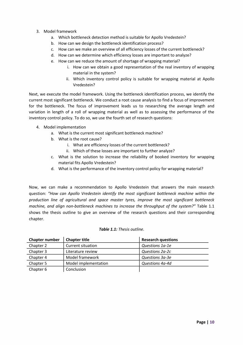
2.2.1 Mixing
A rubber compound is formed by mixing rubber, carbon black, sulphur and other materials using
gigantic mixers. Additional heating and friction are applied to the batch to soften the rubber and
evenly distribute the chemicals. The chemical composition of each batch depends on the tyre part.
So certain rubber formulations are used for the body, other formulas for the beads, and others for
the tread. Although it sounds simple, mixing is actually quite complicated and has to be done several
times. Figure 2.2 represents the mixing process.
Figure 2.2: The mixing process. Reprinted from “The Unofficial Global Manufacturing Trainee Survival
Book”, by Apollo Vredestein B.V., 2015.
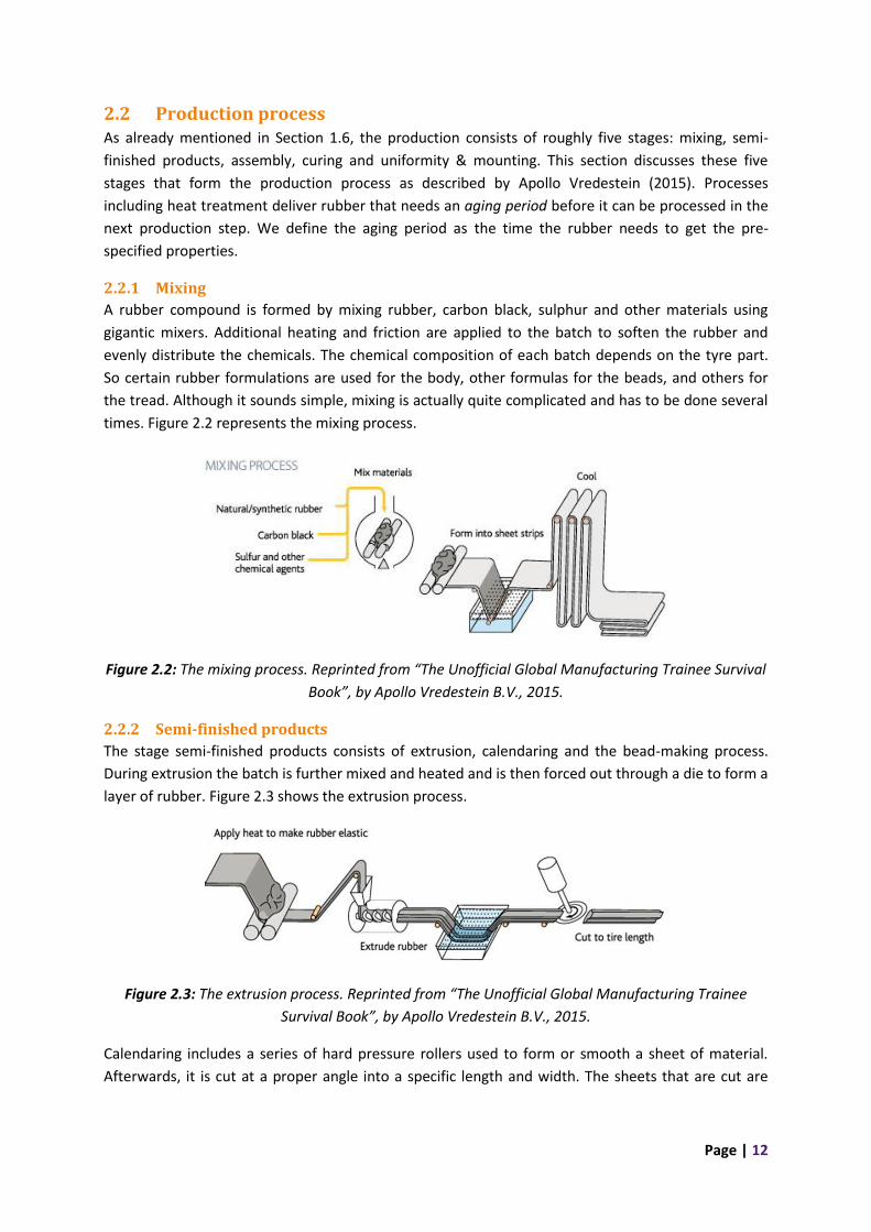
2.2.2 Semi-finished products
The stage semi-finished products consists of extrusion, calendaring and the bead-making process.
During extrusion the batch is further mixed and heated and is then forced out through a die to form a
layer of rubber. Figure 2.3 shows the extrusion process.
Figure 2.3: The extrusion process. Reprinted from “The Unofficial Global Manufacturing Trainee
Survival Book”, by Apollo Vredestein B.V., 2015.
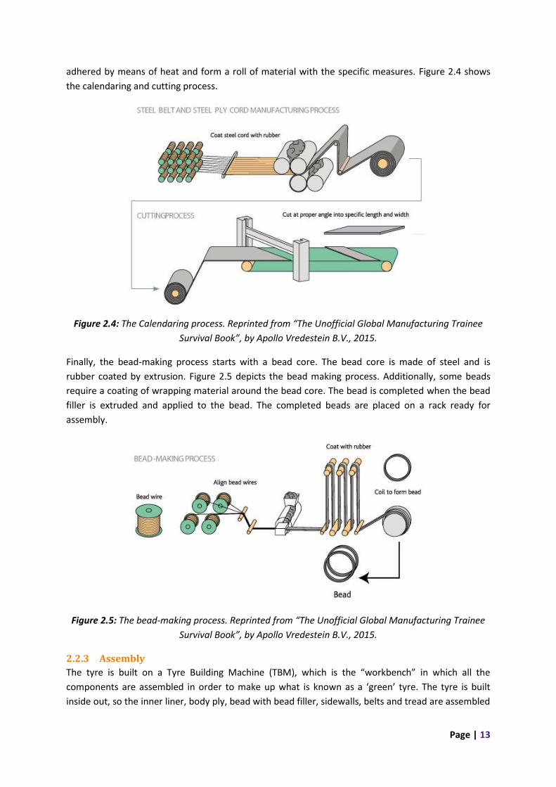
Calendaring includes a series of hard pressure rollers used to form or smooth a sheet of material.
Afterwards, it is cut at a proper angle into a specific length and width. The sheets that are cut are
Page | 13
adhered by means of heat and form a roll of material with the specific measures. Figure 2.4 shows
the calendaring and cutting process.
Figure 2.4: The Calendaring process. Reprinted from “The Unofficial Global Manufacturing Trainee
Survival Book”, by Apollo Vredestein B.V., 2015.
Finally, the bead-making process starts with a bead core. The bead core is made of steel and is
rubber coated by extrusion. Figure 2.5 depicts the bead making process. Additionally, some beads
require a coating of wrapping material around the bead core. The bead is completed when the bead
filler is extruded and applied to the bead. The completed beads are placed on a rack ready for
assembly.
Figure 2.5: The bead-making process. Reprinted from “The Unofficial Global Manufacturing Trainee
Survival Book”, by Apollo Vredestein B.V., 2015.
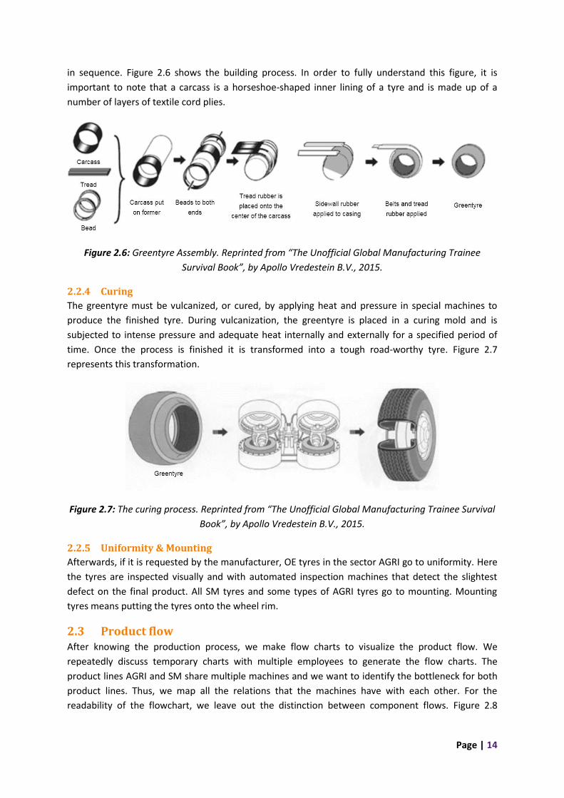
2.2.3 Assembly
The tyre is built on a Tyre Building Machine (TBM), which is the “workbench” in which all the
components are assembled in order to make up what is known as a ‘green’ tyre. The tyre is built
inside out, so the inner liner, body ply, bead with bead filler, sidewalls, belts and tread are assembled
Page | 14
in sequence. Figure 2.6 shows the building process. In order to fully understand this figure, it is
important to note that a carcass is a horseshoe-shaped inner lining of a tyre and is made up of a
number of layers of textile cord plies.
Figure 2.6: Greentyre Assembly. Reprinted from “The Unofficial Global Manufacturing Trainee
Survival Book”, by Apollo Vredestein B.V., 2015.
2.2.4 Curing
The greentyre must be vulcanized, or cured, by applying heat and pressure in special machines to
produce the finished tyre. During vulcanization, the greentyre is placed in a curing mold and is
subjected to intense pressure and adequate heat internally and externally for a specified period of
time. Once the process is finished it is transformed into a tough road-worthy tyre. Figure 2.7
represents this transformation.
Figure 2.7: The curing process. Reprinted from “The Unofficial Global Manufacturing Trainee Survival
Book”, by Apollo Vredestein B.V., 2015.
2.2.5 Uniformity & Mounting
Afterwards, if it is requested by the manufacturer, OE tyres in the sector AGRI go to uniformity. Here
the tyres are inspected visually and with automated inspection machines that detect the slightest
defect on the final product. All SM tyres and some types of AGRI tyres go to mounting. Mounting
tyres means putting the tyres onto the wheel rim.
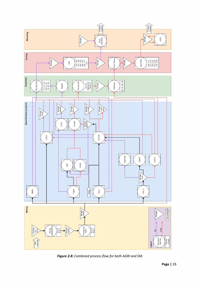
2.3 Product flow After knowing the production process, we make flow charts to visualize the product flow. We
repeatedly discuss temporary charts with multiple employees to generate the flow charts. The
product lines AGRI and SM share multiple machines and we want to identify the bottleneck for both
product lines. Thus, we map all the relations that the machines have with each other. For the
readability of the flowchart, we leave out the distinction between component flows. Figure 2.8
Page | 15
Figure 2.8: Combined process flow for both AGRI and SM.
Page | 16
represents the flowchart for AGRI and SM. Here, the red arrows represent the AGRI line, the purple
arrows represent the SM line and black arrows indicate that both lines travel in that direction. There
are multiple components per product line that follow different routes, which means that multiple
arrows (from the same product line) can leave an operation/machine or storage. We divide the
columns in the production stages from Figure 1.10. These flow charts include the stage uniformity &
mounting for transparency even though they are out of the scope. The flowchart contains names
that are not important for the reader. These names are how employees at Vredestein call the
operations, machines or storage places. If there are multiple machines that execute the same
operation, they are indicated in the cell below the operation. For instance, there are two machines,
Mixer 6 and Mixer 8, that execute the operation called mixing masterbatch. If there is only one
machine to execute an operation, the name in the flowchart refers to the machine name and there is
no cell below the machine. Also, we look at the flowcharts with distinction between component
flows. For the readability of the flowchart, we make separate flow charts per product type
(AGRI/SM), see Appendix 1. Here, the column “semi-finished product” contains flows for different
components that are presented with a specific arrow layout to develop understanding of the flow
per component.
2.4 Production planning Vredestein uses material requirements planning (MRP) as a production planning, scheduling and
inventory control system to manage their manufacturing processes. MRP is a push system since it
computes schedules of what should be started (or pushed) into production based on demand (Hopp
& Spearman, 2011). The process starts with a request from sales. A request from sales is usually
based on a forecast (make-to-stock), but can also be based on an order (make-to-order). Sales has an
annual plan containing all order quantities per time period for all end items (i.e. tyre types). The
annual plan is known in literature as the master production schedule (MPS). It gives the quantity and
due dates for all demand of finished products. The MPS is updated throughout the year with new
information. MRP uses this information to obtain the gross requirements that initiate the MRP
procedure. MRP works backward from the MPS to derive schedules for the components. The bill of
materials (BOM) specifies the relationship between the end product and the components. Using the
BOM, a curing plan is based on the MPS, a building plan is based on the curing plan, etc. There are
exceptions for processes that have a long lead time. The exceptions are the purchase of raw material
and orders for mixtures. The purchase of raw materials is based on the MPS. As suppliers have a long
delivery lead time, the plan is made far ahead of time, matching the delivery lead time. The order for
mixtures is based on the curing plan. The mixing department delivers rubber that needs an aging
period before it can be processed in the next production step. The aging period makes mixing a
production process that is not flexible. This results in the mixing plan being based on the curing plan
and not on the succeeding process. To account for uncertainty and randomness they use a safety
lead time. Applying a safety lead time means that the material should be delivered a certain amount
of time prior to when it is scheduled for usage. The safety lead time is set per department and
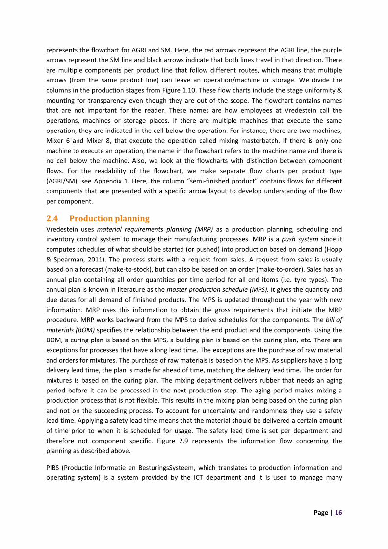
therefore not component specific. Figure 2.9 represents the information flow concerning the
planning as described above.
PIBS (Productie Informatie en BesturingsSysteem, which translates to production information and
operating system) is a system provided by the ICT department and it is used to manage many
Page | 17
Figure 2.9: Information and product flow with regard to the planning. Adapted from “Plannings-
optimalisatie van de productieplanning van Apollo Vredestein B.V.”, by Cornelissen, J., 2019.
processes in the plant. Among other things, the MRP is made in PIBS. A request is registered into PIBS
as an amount of tyres of type x to be finished on date t. PIBS then calculates throughout the system
what resources are needed at each step of the production process to be able to finish this on time.
This means that in the planning, curing is seen as the bottleneck and the other plans are based on the
desired output from curing. PIBS communicates the planning to the machines or operators, and it
contains all product specifications. PIBS is also used to document historical production data. Thus,
after every shift of eight hours the amount of tyres produced and the losses occurred (in minutes per
category) are documented. Then, the plan is revised with the information of the past 8 hours.
To determine the amount of tyres that can be produced in a shift the standard time is used. Within
Apollo Vredestein standard time is defined as: “the time required to produce a qualitative (specified
per product) good product at a workstation with the following conditions:
1. A qualified, average skilled operator working in normal pace,
2. Working on operational released equipment according technical specifications
3. Doing a specific task/s by using pre-scribed tools and following valid standards”
The standard time consists of the machine cycle time and frequential time. The machine cycle time is
the sum of all cyclical activities, i.e. activities that are always executed at that station to manufacture
each product. The frequential time is the time of the activities not performed in all cycles, but in a
certain frequency (such as the exchange of cassettes), and are part of the process. The frequential
time is partially calculated by multiplying the time of the activity by its frequency and partially by
applying a correction rate(%) for unaccounted delays or activities.
2.5 Intermediate stock PIBS also tracks intermediate stock for some SKUs. Thus, it is possible to monitor the current
inventory of a certain SKU within PIBS. This is managed by scanning SKUs after certain activities.
Picking up and delivering SKUs is registered to keep track of the location of the SKUs. At the machine,
using a SKU and the amount that is left over from using a SKU are scanned to make sure the available
stock in the plant is the same as in the system. The other SKUs that are not tracked are also
registered in the system, but the location of these items is not available.
Depending on the type of product, SKUs are stored at an intermediate stock or directly transported
to the next machine. The safety lead time, aging period, and batch size generate a need for storage
Page | 18
space. Thus, the stock that is available consists of SKUs that are ready x hours (i.e. the safety lead
time) before they are needed in production and SKUs that have an aging period. The exception is the
stock of mixtures and the stock of calendar rolls. Large amounts are produced in successive batches
to reduce the amount of waste. This means that the minimum amount produced is larger than the
amount defined by the orders. Thus, the stock level is defined by large residues from production runs
and order related SKUs. The triangles in the flowchart from Figure 2.8 represent all intermediate
stock. If there is no intermediate stock in the flowchart it means that each subsequent machine has
its own (small) storage place. There are two storage spaces for a specific machine registered in PIBS
as separate intermediate stock, because they are bigger storage spaces. This the stock in front of the
ORION and VPA (SM preassembly). Figure 2.8 does not present those stocks, because they are linked
to a specific machine.
Currently, the business teams strive to have a certain amount of production hours (equal to the
safety lead time) in stock. This is defined as a total and does not specify the variety of the stock.
There is a maximum level of stock defined by the space available, by a self-defined limit or by the
material handling equipment (MHE). Many products use specific MHE, which means that if all MHE of
a specific product is occupied, no new products can be produced.
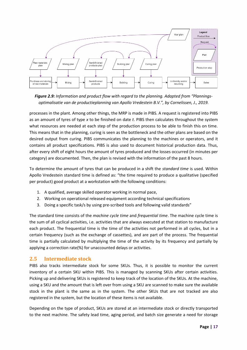
2.6 System performance The system performance regarding TOC can be measured by the percentage of time that there are
no greentyres (NGT) at the curing department. As we mentioned in Section 2.4, Apollo Vredestein
plans on the curing department, which means that all starvation losses at curing result in lost tyres
that could have been sold. NGT is the only starvation loss that occurs at the curing department. Thus,
a low percentage of NGT reflects a good performance of the system. Figure 2.10 gives an overview of
the starvation time (NGT) at the curing department per week for AGRI and SM (%). The time frame of
the figure corresponds with the time frame that we use in Chapter 5 to perform the bottleneck
identification. The average starvation during that period at the curing department was 8.5%. This
means that on average 8.5% of the time that a machine in the curing department is available, it
cannot produce because it has no input materials. The starvation per week for all machines varies
between an average of 2.8% and 14.0%. The division of starvation among the machines in the curing
department is currently unknown, because they are booked as one group of machines.
Figure 2.10: Starvation time at the curing department per week for AGRI and SM (%).
A lower NGT percentage can mean three things. First, the throughput of the system has increased.
The building department delivers more tyres at the right time. This turns a part of the time a machine
is idle into time the machine is producing. Thus, the throughput of the system increases. Second, the
planning is adjusted to the bottleneck. The curing department lowers their demand, making it
possible for the building department to deliver more tyres (%) at the right time. Thus, the NGT
Page | 19
percentage decreases. This results in a more realistic demand throughout the plant, improving the
flow. Over-demanding the system results in more rush orders and changeovers disturbing the
planning. In practice that means that an improved flow also leads to an increase in throughput. Third,
the decision is made to use operators from the curing department to focus on another part of
production. This decision is only made if another process has a large breakdown or other issues that
are expected to lead to large shortages at succeeding processes and finally starvation at the curing
department. This decision will lower the NGT and result in the highest possible throughput in that
situation. Thus, all three possibilities that result in a lower NGT are positive for the throughput of the
system. In theory, a lower NGT can also be accomplished by adjusting the planning below the
capacity of the system. In practice, this will never happen, because Vredestein steers on the MPS and
numbers produced.
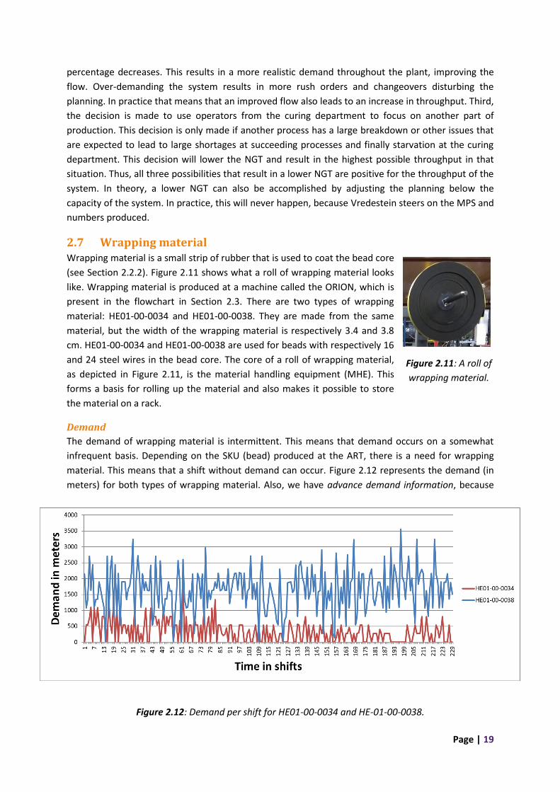
2.7 Wrapping material Wrapping material is a small strip of rubber that is used to coat the bead core
(see Section 2.2.2). Figure 2.11 shows what a roll of wrapping material looks
like. Wrapping material is produced at a machine called the ORION, which is
present in the flowchart in Section 2.3. There are two types of wrapping
material: HE01-00-0034 and HE01-00-0038. They are made from the same
material, but the width of the wrapping material is respectively 3.4 and 3.8
cm. HE01-00-0034 and HE01-00-0038 are used for beads with respectively 16
and 24 steel wires in the bead core. The core of a roll of wrapping material,
as depicted in Figure 2.11, is the material handling equipment (MHE). This
forms a basis for rolling up the material and also makes it possible to store
the material on a rack.
Demand
The demand of wrapping material is intermittent. This means that demand occurs on a somewhat
infrequent basis. Depending on the SKU (bead) produced at the ART, there is a need for wrapping
material. This means that a shift without demand can occur. Figure 2.12 represents the demand (in
meters) for both types of wrapping material. Also, we have advance demand information, because
Figure 2.12: Demand per shift for HE01-00-0034 and HE-01-00-0038.
Figure 2.11: A roll of
wrapping material.
Page | 20
the demand is created by Vredestein. Advance demand information for a product is obtained when
customers place orders in advance for a future delivery (Özer & Wei, 2004). Thus, the demand
requested in future period t is given prior to period t, where one period equals to one shift. This
means that we do not have external demand uncertainty.
Order system
The wrapping material has a fixed order quantity. The material comes originally from the machine
called KAL4, where the slaps of rubber are calendared. This is done in large batches, because there
are large setup costs related to scrap. After KAL4, the large rolls (Calendar rolls) are cut in two at the
machine called the Calemard and finally the ORION cuts the rolls in smaller pieces with a specific
width resulting in the desired SKU. Because the rolls of wrapping material are cut out of half a
calendar roll, the calendar roll defines the batch size that leaves the ORION. Thus, the ORION has a
fixed order quantity that can be ordered multiple times. However, due to scrap at the calendar
process the width of the calendar roll can vary slightly. Also, the length of the roll is influenced by
scrap at the Calemard and ORION. The length of a roll varies among batches, but is usually the same
for all rolls within a batch. Thus, the order quantity per roll is fixed and equals 250 meters, but the
amount that the ORION delivers fluctuates. This is internal demand uncertainty, which we explain in
Section 3.3.1. When an order is placed, there is a lead time of 4 to 8 hours depending on the queue
waiting time. This is internal supply uncertainty, which we explain in Section 3.3.1. The ORION
produces for multiple machines, which creates fluctuations in lead time depending on the schedule.
There is no agreement or contract on the lead time, because it is within Vredestein. If necessary, the
wrapping material can be ordered with emergency. In case of emergency, there is a lead time of one
hour.
Inventory
Because there is a fixed order quantity, there usually is cycle stock. The cycle stock is a result of
producing or ordering in larger quantities than one unit at a time. The amount of inventory that
results from these batches is called cycle stock. Also, when ordering wrapping material a safety lead
time of two hours is applied. This means that the material needs to be delivered two hours prior to
when it is scheduled for usage. This creates an amount of stock depending on the demand. The two-
hour safety lead time is a general safety lead time applied to all orders in the semi-finished products
department. Thus, it is not based on the uncertainties at the ORION. Furthermore, the wrapping
material has a limited shelf life. The material has a shelf life of one month. If the material is older
than one month, it has to be disposed of. The material is stored at the ART on a rack. There are two
(different) racks that together can carry up to 126 rolls (of max. 250 meters) of wrapping material.
For calculating the available storage capacity, we do not differentiate between HE01-00-0034 and
HE01-00-0038, because the MHE has a width of 4.0 cm. Thus, the width of the MHE defines the
storage capacity.
2.8 Conclusion In this chapter we analyzed the current situation at Vredestein. In Section 2.1, we have given insight
in the tyre structure and the components that are used to build a tyre. The production process is
covered in Section 2.2 and consists of several steps. This section explains the departments and its
processes that form the production process. To show how the production steps are linked to each
other, we mapped the product flow in Section 2.3. To be able to produce they have to make a
production planning, which we explained in Section 2.4. Vredestein uses material requirements

Page | 21
planning (MRP) as a production planning, scheduling and inventory control system to manage their
manufacturing processes. They add safety lead times to buffer against uncertainty. They use PIBS to
manage all processes in the plant and among other things, the MRP is made in PIBS. We mentioned
intermediate stock in Section 2.5. They also use PIBS to track inventory. The safety lead time, aging
period and batch sizes generate a need for storage space. We described the performance of the
system in Section 2.6. We can be measure the performance of the system with the percentage of no
greentyres (NGT) at the curing department. In practice, a lower NGT percentage is positive for the
throughput of the system. Finally, in Section 2.7 we gave more specific information for wrapping
material about the previously mentioned topics.

Page | 22
Page | 23
3. Literature review In this chapter we discuss some relevant findings in literature. Section 3.1 presents an overview of
the main operations management philosophies to improve the manufacturing performance. Section
3.2 gives an overview of the bottleneck identification methods that are currently known in literature.
Section 3.3 gives information about inventory control and the steps to systematically establish
inventory policies.
3.1 Operations management philosophies There are multiple operations management philosophies proposed in literature to improve the
manufacturing performance. This section elaborates on the most common approaches: total quality
management, business process re-engineering, lean manufacturing, theory of constraints and six
sigma. This overview is based on the descriptions from Slack, Brandon-Jones, and Johnston (2016).
3.1.1 Total quality management (TQM)
This approach puts quality, and improvement generally at the heart of everything that is done by an
operation. TQM achieves this by focusing on the following elements:
• Meeting the needs and expectations of customers
• Improvement covers all parts of the organization and every person in the organization.
• Including all costs of quality
• Getting things right the first time: designing in quality rather than inspecting it in.
• Developing the systems and procedures that support improvement.
3.1.2 Business process re-engineering (BPR)
BPR is based on the idea that, rather than using technology to automate work, it is better to remove
the need for work in the first place. This can also be summarized as “do not automate, obliterate”.
This approach strives for dramatic improvements in performance by radically rethinking and
redesigning the process.
3.1.3 Lean manufacturing (LM)
The focus of lean manufacturing is to achieve a flow of materials, information and customers that
deliver exactly what customers want, in exact quantities, exactly when needed, exactly where
required and at the lowest possible cost. This is achieved by the elimination of waste in all its forms,
the inclusion of all staff of the operation in its improvement and the idea that all improvement
should be on a continuous basis. LM uses a pull control, where the pace and specification of what is
done are set by the ‘customer’ workstation.
3.1.4 Theory of Constraints (TOC)
Theory of Constraints (TOC) focuses the attention on the capacity constraints or bottleneck parts of
the operation. Here, a constraint is defined as anything that limits the system from achieving higher
performance relative to its goal. TOC emphasizes a five steps process of ongoing improvement. One
major assumption in TOC is that the measurements—throughput, inventory and operating
expenses—can measure the goal of an organization, and everything else is derived logically from that
assumption.

Page | 24
3.1.5 Six sigma (SiS)
Six Sigma is “A disciplined methodology of defining, measuring, analyzing, improving, and controlling
the quality in every one of the company’s products, processes and transactions - with the ultimate
goal of virtually eliminating all defects” (Slack et al., 2016). This comes from the idea that true
customer satisfaction can only be achieved when its products were delivered when promised, with
no defects, with no early-life failures and when the product did not fail excessively in service.
3.1.6 Discussion
All of the philosophies mentioned strive to improve the systems performance. Even though the
approaches have the same goal, they do emphasize different type of changes. TQM, LM and TOC all
incorporate ideas of continuous improvement, while SiS can be used for small or very large changes
and BPR strives for radical changes. Also, they differ in the aim of the approach. For BPR the focus is
on what should happen rather than how it should happen, while SiS and TQM focus more on how
operations should be improved. The main contribution of TOC versus LM is the idea that the effects
of bottleneck constraints must be prioritized and can excuse inventory if it means maximizing the
utilization of the bottleneck. If demand is suddenly far greater than expected for certain products,
the LM system may be unable to cope. Pull scheduling is a reactive concept that works best when
independent demand has been levelled and dependent demand synchronized. While lean
synchronization may be good at control, it is weak on planning.
3.2 Bottleneck identification methods The term bottleneck identification refers to the research of where in the production line a process
restrains the overall output. During the last decades, several bottleneck identification methods have
been proposed in literature. These methods vary from analytical or simulation to data driven. Some
of them are detecting a real-time bottleneck while most focus on a long-term bottleneck. Also, the
system matching the method varies. In this section, we describe the most common methods known
in literature.
3.2.1 Process time
This method measures the process times, or cycle time, and with that detects the capacity limit. In
case of a flow shop, the machine with the longest cycle time would have the lowest capacity and
therefore be the bottleneck (Kuo et al., 1996). This is a very fast and simple way to identify the
bottleneck. The downside is that it does not include any losses or variability and therefore does not
necessarily represent the true bottleneck. It merely shows the maximum capacity of the production
line under ideal conditions. Also, this method works best for systems with one machine per station
and constant cycle times.
3.2.2 Utilization
The utilization method knows multiple variations depending on the definition of utilization. For
instance, Betterton & Silver (2012) define the utilization as the percentage of time the resource is not
idle due to lack of work. Thus, utilization is calculated as the time spent producing divided by the
effective process time, excluding setups or breakdowns. Because of this, it is also known as the
effective process time method. On the other hand, Roser et al. (2003) define utilization as the
percentage of time a resource is active. Here, active means that the resource is not waiting (i.e.
working, breakdown, under repair, regular maintenance, changeover, etc.). Thus, utilization is
calculated as the time a resource is active divided by the total time. All methods agree that in a serial

Page | 25
line, the machine with the largest utilization is considered to be the bottleneck. As this method is
based on averages it cannot detect shifting bottlenecks (see Section 1.3) in dynamic systems. The
utilization method is comparable to the process time method, but it does take losses into account.
The losses that are taken into account depend on the definition used. In contrary with the process
time method, this method can be used on systems with varying cycle times because it uses
aggregated times.
3.2.3 Inventory based methods
There are multiple methods that use the inventories between processes to detect the bottleneck
(Roser & Nakano, 2015). This can be based on the queue length or the waiting time in queue. The
longest waiting time method states that the station where work waits the longest is the bottleneck.
This is measured by the maximum time a job spends in queue. The longest queue method identifies
the station that has the greatest number of waiting jobs in queue for the largest proportion of the
overall line processing period as the bottleneck. Both methods also have an average version, the
average waiting time method and the maximum average queue length. Respectively measured by
the average time a job spends in queue and the largest average number of waiting jobs in queue.
3.2.4 Arrow method
Li and Meerkov (2009) describe the arrow method that is based on blockage and starvation
probabilities. Process blocking occurs when a process must stop because its subsequent buffer or
process is full. This causes the preceding process to stop until the work in process (WIP) is cleared.
Process starvation occurs when the preceding buffer or process is empty, meaning there is no supply
of materials (Roser, Lorentzen, & Deuse, 2014). Thus, blockage probability is the percentage of the
available time the machine is idle, because it has no production plan. This means that it has no order
to produce or has reached a sufficient level of stock. Starvation probability is the percentage of the
available time the machine is idle, because it is waiting for parts from upstream. If the machine
blockage and starvation probabilities, respectively 𝑚𝑏𝑖 and 𝑚𝑠𝑖 for each station 𝑖, are known, this
method can identify the location of the bottleneck in serial production lines.
If:
𝑚𝑏𝑖 > 𝑚𝑠𝑖+1: 𝑖 = 1, … , 𝑀 − 1
Where 𝑀 is the number of machines in the production line. Then, the bottleneck is downstream
stage 𝑖 and thus an arrow is drawn from station 𝑖 to 𝑖 + 1.
If:
𝑚𝑏𝑖 < 𝑚𝑠𝑖+1: 𝑖 = 2, … , 𝑀
Then, the bottleneck is upstream of stage 𝑖 + 1, and an arrow is drawn from 𝑖 + 1 to 𝑖. The machine
with no departing arrows is identified as the bottleneck.
If there are multiple machines detected as the bottleneck, the machine that is detected as a
bottleneck and has the highest bottleneck severity is the bottleneck. Bottleneck severity is defined as:
𝑆1 = 𝑚𝑠2 − 𝑚𝑏1, 𝑆𝑀 = 𝑚𝑏𝑀−1 − 𝑚𝑠𝑀
𝑆𝑖 = (𝑚𝑏𝑖−1 − 𝑚𝑠𝑖+1) − (𝑚𝑏𝑖 − 𝑚𝑠𝑖) ∶ 𝑖 = 2, … , 𝑀 − 1

Page | 26
All formulas mentioned above can be found in Li and Meerkov (2009).
3.2.5 Turning point method
The turning point method (TPM) is developed by Li et al. (2007). Just like with the arrow method,
TPM uses machine blockage and starvation times as a percentage of the total time per machine,
respectively 𝑇𝐵𝑖 (%) and 𝑇𝑆𝑖 (%), for each station 𝑖 to identify the location of the bottleneck.
Blockage time is the percentage of the available time the machine is idle, because it has nothing to
produce. This means that it has no order to produce or has reached a sufficient level of stock.
Starvation time is the percentage of the available time the machine is idle, because it is waiting for
parts from upstream. The TPM method makes two observations:
The first observation is that stations upstream from the bottleneck are blocked and stations
downstream from the bottleneck are starved. This results in a positive 𝑇𝐵𝑖 − 𝑇𝑆𝑖 for its upstream
stations and a negative 𝑇𝐵𝑖 − 𝑇𝑆𝑖 for its downstream stations. This makes the bottleneck station a
“turning point”.
The second observation is that a bottleneck station is neither starved nor blocked. This means that
the total blockage and starvation time of a bottleneck station (𝑇𝐵𝑗 + 𝑇𝑆𝑗) should be smaller than the
upstream and downstream stations.
Therefore, machine 𝑚𝑗 is the turning point if all of the following equations are satisfied:
𝑇𝐵𝑖 − 𝑇𝑆𝑖 > 0: 𝑖 = 1, … , 𝑗 − 1, 𝑗 ≠ 1, 𝑗 ≠ 𝑀,
𝑇𝐵𝑖 − 𝑇𝑆𝑖 < 0: 𝑖 = 𝑗 + 1, … , 𝑀, 𝑗 ≠ 1, 𝑗 ≠ 𝑀,
𝑇𝐵𝑗 + 𝑇𝑆𝑗 < 𝑇𝐵𝑗−1 + 𝑇𝑆𝑗−1, 𝑗 ≠ 1, 𝑗 ≠ 𝑀,
𝑇𝐵𝑗 + 𝑇𝑆𝑗 < 𝑇𝐵𝑗+1 + 𝑇𝑆𝑗+1, 𝑗 ≠ 1, 𝑗 ≠ 𝑀,
If 𝑗 = 1,
𝑇𝐵1 − 𝑇𝑆1 > 0 𝑎𝑛𝑑 𝑇𝐵2 − 𝑇𝑆2 < 0
𝑎𝑛𝑑 𝑇𝐵1 + 𝑇𝑆1 < 𝑇𝐵2 + 𝑇𝑆2
If 𝑗 = 𝑀,
𝑇𝐵𝑀−1 − 𝑇𝑆𝑀−1 > 0 𝑎𝑛𝑑 𝑇𝐵𝑀 − 𝑇𝑆𝑀 < 0
𝑎𝑛𝑑 𝑇𝐵𝑀 + 𝑇𝑆𝑀 < 𝑇𝐵𝑀−1 + 𝑇𝑆𝑀−1
See Li et al. (2007) for the details.
If there are multiple machines detected as the bottleneck, the machine that is detected as a
bottleneck with the maximum bottleneck index is the bottleneck. Where bottleneck index is defined
as:
𝐼1 =𝑇𝑆
𝑇𝐵1 + 𝑇𝑆1, 𝐼𝑀 =
𝑇𝐵𝑀−1
𝑇𝐵𝑀 + 𝑇𝑆𝑀,
Page | 27
𝐼𝑖 =𝑇𝐵𝑖−1 + 𝑇𝑆𝑖+1
𝑇𝐵𝑖 + 𝑇𝑆𝑖: 𝑖 = 2, … , 𝑀 − 1
For details of the bottleneck index, see Yu and Matta (2014). This method can be used to detect the
bottleneck in serial production lines as well as complex serial manufacturing systems.
3.2.6 Active period method
The active period method (Roser, Nakano, & Tanaka, 2002) is based on the duration that a machine is
in active mode. The active mode includes the time it produces parts, is faulted, has a tool change etc.
If the machine becomes idle, the active mode changes into inactive. The momentary (or real-time)
bottleneck is the machine with the longest uninterrupted active time. The average active period
method defines the bottleneck as the process with the longest average active period. This results in a
non-momentary bottleneck. These methods are able to determine the overall effect of the processes
on system capacity. This method distinguishes between the time the machine is a sole bottleneck
and a shifting bottleneck. It is a flexible method and can be used in a wide variety of systems. A
drawback is that it does require extensive process-related data. As a result, this method is only useful
if the data is available.
3.2.7 The bottleneck walk
The bottleneck walk (Roser, Lorentzen, & Deuse, 2014) is based on the active period method while
avoiding the extensive data requirement. While you walk through the process, you observe the
process flow and monitor the data of processes being starved and blocked, and inventory levels. The
inventories tend to be full upstream and empty downstream the bottleneck. The state of a process,
being starved or blocked, gives more accuracy as a process can never be a bottleneck while it is
waiting for another process. If the analysis is made frequently, a shifting bottleneck can be detected.
For this method to work, the inventory levels have to be visible at any time. Visible queueing means
that you have to be able to distinguish the items in stock. Also, visible queueing is only applicable to
processes with a single queue for one given resource.
3.2.8 Simulation based
Many real-world systems are too complex (both in terms of size and stochasticity) to be described by
analytical functions or equations. Using a simulation model (Lemessi et al., 2012), it is possible to
simulate the behavior of such a system. Knowledge about the system and accurate data are vital to
build an accurate model. This means that the output of the model can be only as good as the input of
the model. The transformation of inputs to outputs makes simulation models interesting as they can
provide answers to “What if?” questions. The downsides are that it is very time consuming to make a
simulation model and perform a simulation. Also, it is expensive to keep the simulation model up to
date with the changes in the production system.
3.2.9 Bottleneck identification method summary
When choosing a method, a trade-off has to be made. We create a table containing their
characteristics to be able to compare the methods, see Table 3.1. After researching the current
situation in the next chapter, we use this table to filter the methods and choose one or more
methods that fit the situation.
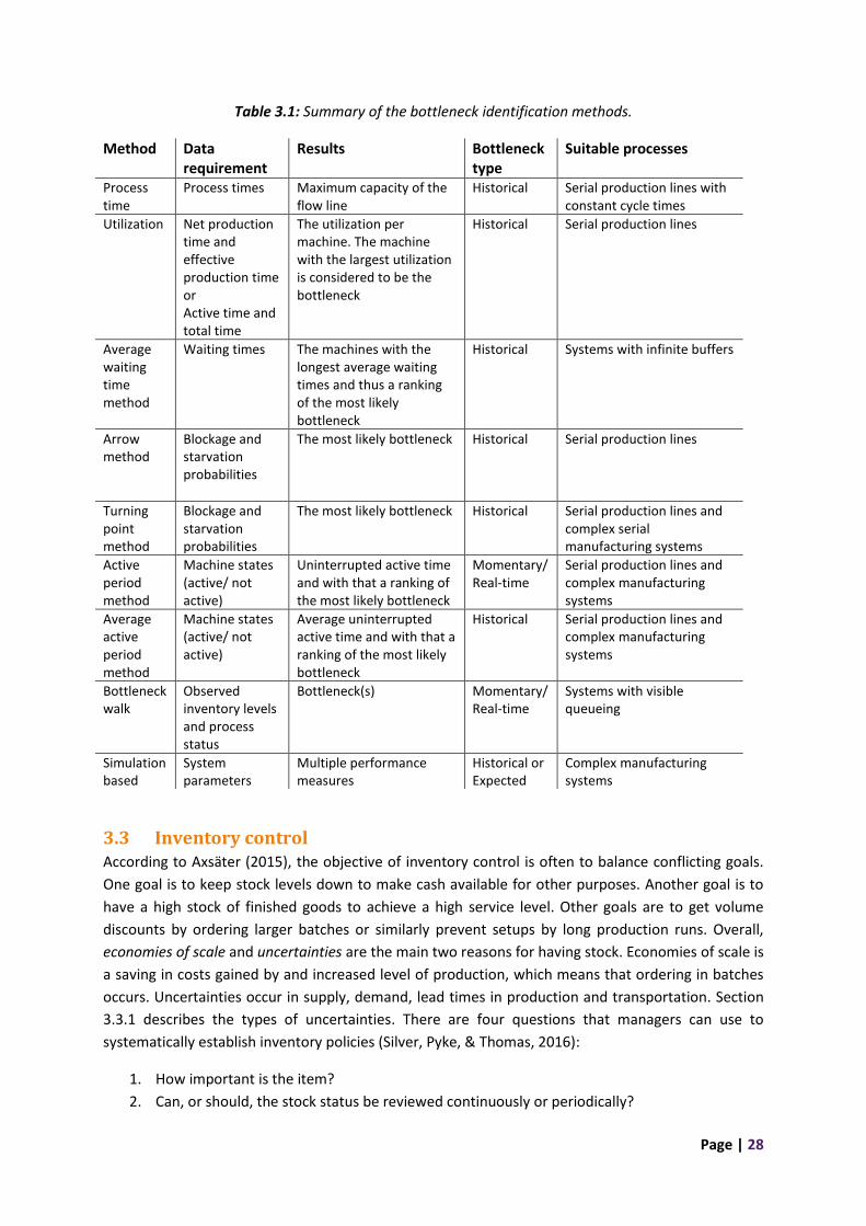
Page | 28
Table 3.1: Summary of the bottleneck identification methods.
Method Data requirement
Results Bottleneck type
Suitable processes
Process time
Process times
Maximum capacity of the flow line
Historical Serial production lines with constant cycle times
Utilization Net production time and effective production time or Active time and total time
The utilization per machine. The machine with the largest utilization is considered to be the bottleneck
Historical Serial production lines
Average waiting time method
Waiting times The machines with the longest average waiting times and thus a ranking of the most likely bottleneck
Historical Systems with infinite buffers
Arrow method
Blockage and starvation probabilities
The most likely bottleneck Historical Serial production lines
Turning point method
Blockage and starvation probabilities
The most likely bottleneck Historical Serial production lines and complex serial manufacturing systems
Active period method
Machine states (active/ not active)
Uninterrupted active time and with that a ranking of the most likely bottleneck
Momentary/ Real-time
Serial production lines and complex manufacturing systems
Average active period method
Machine states (active/ not active)
Average uninterrupted active time and with that a ranking of the most likely bottleneck
Historical Serial production lines and complex manufacturing systems
Bottleneck walk
Observed inventory levels and process status
Bottleneck(s) Momentary/ Real-time
Systems with visible queueing
Simulation based
System parameters
Multiple performance measures
Historical or Expected
Complex manufacturing systems
3.3 Inventory control According to Axsäter (2015), the objective of inventory control is often to balance conflicting goals.
One goal is to keep stock levels down to make cash available for other purposes. Another goal is to
have a high stock of finished goods to achieve a high service level. Other goals are to get volume
discounts by ordering larger batches or similarly prevent setups by long production runs. Overall,
economies of scale and uncertainties are the main two reasons for having stock. Economies of scale is
a saving in costs gained by and increased level of production, which means that ordering in batches
occurs. Uncertainties occur in supply, demand, lead times in production and transportation. Section
3.3.1 describes the types of uncertainties. There are four questions that managers can use to
systematically establish inventory policies (Silver, Pyke, & Thomas, 2016):
1. How important is the item?
2. Can, or should, the stock status be reviewed continuously or periodically?
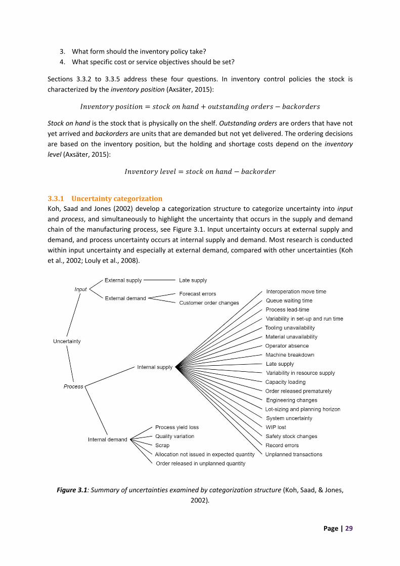
Page | 29
3. What form should the inventory policy take?
4. What specific cost or service objectives should be set?
Sections 3.3.2 to 3.3.5 address these four questions. In inventory control policies the stock is
characterized by the inventory position (Axsäter, 2015):
𝐼𝑛𝑣𝑒𝑛𝑡𝑜𝑟𝑦 𝑝𝑜𝑠𝑖𝑡𝑖𝑜𝑛 = 𝑠𝑡𝑜𝑐𝑘 𝑜𝑛 ℎ𝑎𝑛𝑑 + 𝑜𝑢𝑡𝑠𝑡𝑎𝑛𝑑𝑖𝑛𝑔 𝑜𝑟𝑑𝑒𝑟𝑠 − 𝑏𝑎𝑐𝑘𝑜𝑟𝑑𝑒𝑟𝑠
Stock on hand is the stock that is physically on the shelf. Outstanding orders are orders that have not
yet arrived and backorders are units that are demanded but not yet delivered. The ordering decisions
are based on the inventory position, but the holding and shortage costs depend on the inventory
level (Axsäter, 2015):
𝐼𝑛𝑣𝑒𝑛𝑡𝑜𝑟𝑦 𝑙𝑒𝑣𝑒𝑙 = 𝑠𝑡𝑜𝑐𝑘 𝑜𝑛 ℎ𝑎𝑛𝑑 − 𝑏𝑎𝑐𝑘𝑜𝑟𝑑𝑒𝑟
3.3.1 Uncertainty categorization
Koh, Saad and Jones (2002) develop a categorization structure to categorize uncertainty into input
and process, and simultaneously to highlight the uncertainty that occurs in the supply and demand
chain of the manufacturing process, see Figure 3.1. Input uncertainty occurs at external supply and
demand, and process uncertainty occurs at internal supply and demand. Most research is conducted
within input uncertainty and especially at external demand, compared with other uncertainties (Koh
et al., 2002; Louly et al., 2008).
Figure 3.1: Summary of uncertainties examined by categorization structure (Koh, Saad, & Jones,
2002).

Page | 30
Buffering against uncertainty can be done by using safety stock or safety lead time. Safety stock is the
amount of inventory kept on hand, on average, to allow for the uncertainty of demand and supply in
the short run (Silver et al., 2016). The safety stock levels depend on the desired customer service
level. Safety lead time is the difference between the optimal planned lead time and the lead time on
average over the planning horizon (Molinder, 1997). Thus, the planned lead time equals the
theoretical lead time plus the safety lead time.
Additionally, more accurate forecasting, increased flexibility, and responsiveness are also shown to
effectively mitigating the effects of delivery uncertainties (Chung, Talluri, & Kovács, 2018).
Uncertainty at external supply is mainly caused by failure of external suppliers to deliver as ordered.
There are multiple opinions on how to deal with this type of uncertainty. Whybark and Williams
(1976) suggest that safety stock is more appropriate for buffering quantity uncertainty and safety
lead time for dampening timing uncertainty. However, Grasso and Taylor (1984) prefer safety stock
for both quantity and lead time uncertainties.
Uncertainties in external demand refer to inaccurate forecasts and customer order changes. This
type of uncertainty is extensively researched. To buffer against uncertainty at external demand,
usually safety stock is applied. Also, multiple dampening approaches are examined to reduce the
uncertainty, such as improving the forecast accuracy (Sridharan & LaForge, 1989; Fildes & Kingsman,
1997) or freezing the master production schedule (Sridharan & LaForge, 1994).
Internal supply uncertainty occurs at the supply chain within the manufacturing cycle of the MRP
planned internal manufacture. For example, parts arriving late from the previous workstation due to
machine breakdown, operator absence or tooling unavailability. Vargas and Dear (1991) identify that
safety stock should be used to buffer both internal supply and external demand uncertainties.
Internal demand uncertainty occurs within the demand chain of the manufacturing cycle of the MRP
planned manufacture. An example is variation in quality resulting in part shortages. If the planned
scrap factor is lower than the actual scrap level, a yield loss is encountered. This yield loss will be
reflected at the output of the related workstation, which is mimicked as internal demand. In other
words, there is quantity uncertainty within the output of the workstation. Kurtulus and Pentico
(1988) propose the use of safety stock to buffer process yield loss.
3.3.2 Inventory classification
The first step to systematically establish inventory policies is to establish how critical the item under
consideration is to the firm. Typically, somewhere on the order of 20% of the SKUs account for 80%
of the total annual dollar usage (Silver et al., 2016). This suggests that all SKUs in a firm’s inventory
should not be controlled to the same extent. It is common to classify inventory by means of an ABC
analysis. Class A items should receive the most personalized attention. These are usually the first 5%
to 20% of the SKUs with the highest dollar volume. Class B items have an intermediate dollar volume
and roughly 30% of the total SKUs fall into this category. The remaining items fall into class C. For
these SKUs, the decision system must be kept as simple as possible.
The traditional ABC analysis only includes the value per unit and the sales of the product, together
they form the dollar volume. Using only this criterion, the importance of the SKU to the company is
not taken into account. Multiple extensions of this analysis are researched and include other criteria

Page | 31
such as criticality, sales pattern and commonality (Cohen and Ernst, 1988; Flores and Whybark,
1987).
3.3.3 Continuous versus periodic review
The review interval (R) is the time that elapses between two consecutive moments at which the stock
level is known. How often the inventory status should be determined specifies the review interval.
There are two ways to review inventory: periodically or continuously (Silver et al., 2016). Continuous
review is an extreme case where the stock status is always known. With periodic review the stock
status is determined every R time units. Any time the inventory position is reviewed an order can be
placed. If an order is placed, it will be delivered after a certain lead time (L). The lead time is the time
from the ordering decision until the ordered amount is available on shelf (Axsäter, 2015). A
disadvantage of continuous review in comparison with periodic review is the workload on the staff.
The replenishment decision can be made at any moment in time, which makes the load less
predictable. Usually the staff prefers a rhythmic pattern over a random pattern. With periodic review
items can be grouped and all items within a group can be given the same review interval. Another
disadvantage of continuous review is that it is more expensive for fast movers. Fast movers have
many transactions per unit of time resulting in higher reviewing costs and reviewing errors. However,
for slow movers the reviewing costs are low, because updates are only made when a transaction
occurs. The advantage of continuous review is that it has less uncertainty to the value of the stock
level. The review period (R) is smaller, which means that the period that needs safety protection is
smaller (L versus L+R). Thus, less safety stock is required to attain the same customer service level.
3.3.4 Inventory control policies
After categorizing the item(s) and choosing between continuous or periodic review, we can decide on
the form of the inventory control policy. The inventory control policy determines when an order
should be placed and what quantity should be ordered. Silver et al. (2016) mention four main
inventory control policies for single-echelon systems. Additionally, there is another policy that is
studied exhaustively (Janssen, Heuts, & de Kok, 1996). Table 3.2 summarizes these inventory control
policies. The models below are infinite horizon models. In practice, Vredestein uses a finite planning
horizon for their production. We can still use these models, because in practice the decisions that are
made only include information from the finite planning horizon. This has three reasons. First, in
actual applications a rolling schedule procedure is almost always used, and this is also the case for
Vredestein. Specifically, although replenishment quantities may be computed over the entire
planning horizon, only the most immediate decisions are implemented (Silver et al., 2016). Second,
we look at two types of uncertainties that are short term influences as will be explained in Section
4.4.1. Thus, we do not need to observe the influence of long term changes on safety stock. Third, the
lead time plus review period is smaller than the period with advanced demand information. Thus, the
safety stock buffers for a period within the planning horizon. This means that the decisions that are
made using the infinite model are only including information from the finite planning horizon if a
rolling schedule procedure is implemented.
Table 3.2: Inventory control policies.
Lot size Periodic review Continuous review
Fixed order quantity (R,s,Q) (s,Q)
Variable order quantity (R,S), (R,s,S) (s,S)
Page | 32
In the table R, s, S and Q respectively stand for the review period (or review interval), the reorder
point, the order-up-to level and the order quantity.
(s,Q) policy
The (s,Q) policy is a continuous-review system. If the inventory position drops to the reorder point s
or below, a fixed quantity Q is ordered. The advantages of this policy are that it is quite simple and
the requirements for the supplier are predictable. A downside is that the system cannot cope with
individual transactions that are large. A very large transaction can result in a replenishment of size Q
that does not raise the inventory above the reorder point.
(s,S) policy
The (s,S) policy is also a continuous review system. In contrast to the (s,Q) policy, the (s,S) policy uses
a variable replenishment quantity. If the inventory position drops to the reorder point s, a variable
order quantity is used to raise the inventory position to the order-up-to level S. Note that if all
demand transactions are unit sized, the (s,Q) and (s,S) policies are identical because the
replenishment requisition will always be made when the inventory position is exactly at s, that is, S =
s + Q (Silver et al., 2016). A downside of this policy is the computational effort to find the best values
for s and S. This policy can be preferable for class A items as the potential savings are appreciable. A
disadvantage of the (s,S) policy is the variable order quantity, which has a higher chance for errors
and can be inconvenient from a packaging or handling standpoint.
(R,S) policy
The (R,S) policy is a periodic review system. Every R units of time a variable order quantity is used to
raise the inventory position to the order-up-to level S. This policy is common in companies without
sophisticated computer control. Disadvantages are the varying replenishment quantities and the
higher carrying costs in comparison with the continuous-review system. The system is preferred in
terms of coordinating the replenishments of related items. Thus, it is frequently used when multiple
items are ordered from the same supplier or require resource sharing and the carrying costs can be
reduced.
(R,s,S) policy
The (R,s,S) policy is a combination of the (s,S) and (R,S) policy. Every R units of time the inventory
position is reviewed. If the inventory position is at or below the reorder point s, a variable order
quantity is used to raise it to the order-up-to level S. If the inventory position is above s, no order is
placed until the next review moment. Note that if R = 0 the (s,S) and (R,s,S) policies are identical and
that (R,S) is a special case of (R,s,S) where s = S -1. It has been shown that the best (R,s,S) policy
produces a lower total of replenishment, carrying, and shortage costs than any other system (Silver
et al., 2016). However, obtaining the best policy (i.e. the three control parameters) is a large
computational effort. Thus, this policy is only suitable for A items. Another downside is the variable
order quantity (see the (s,S) policy).
(R,s,Q) policy
The (R,s,Q) policy is a combination of the (R,s,S) and (s,Q) policies. Every R units of time the inventory
position is reviewed. If the inventory position is at or below the reorder point s, an integral multiple
of a fixed quantity Q is used, such that the inventory position is raised to a value between s and s + Q.
If the inventory position is above s, no order is placed until the next review moment. Because it is
possible to order a multiple of Q, this policy is also referred to as the (R,s,nQ) policy (Larsen &
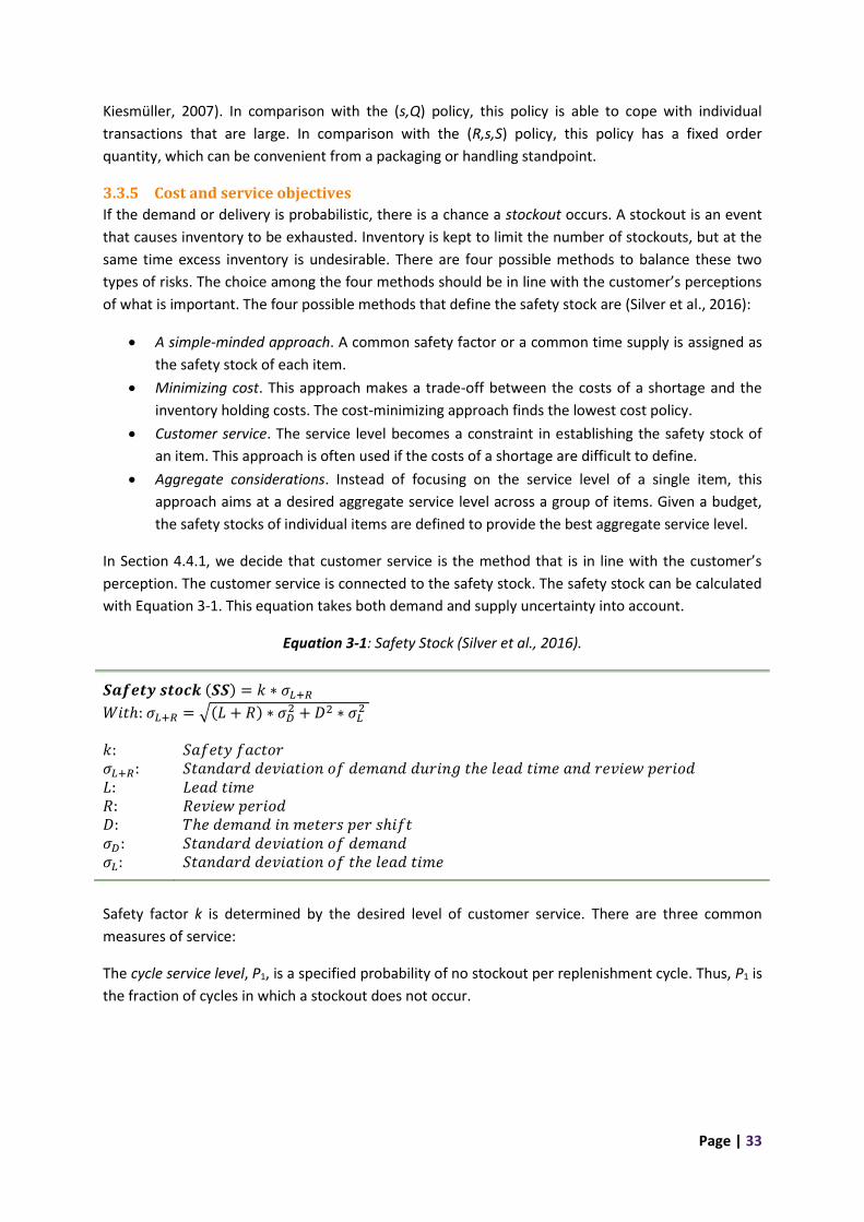
Page | 33
Kiesmüller, 2007). In comparison with the (s,Q) policy, this policy is able to cope with individual
transactions that are large. In comparison with the (R,s,S) policy, this policy has a fixed order
quantity, which can be convenient from a packaging or handling standpoint.
3.3.5 Cost and service objectives
If the demand or delivery is probabilistic, there is a chance a stockout occurs. A stockout is an event
that causes inventory to be exhausted. Inventory is kept to limit the number of stockouts, but at the
same time excess inventory is undesirable. There are four possible methods to balance these two
types of risks. The choice among the four methods should be in line with the customer’s perceptions
of what is important. The four possible methods that define the safety stock are (Silver et al., 2016):
• A simple-minded approach. A common safety factor or a common time supply is assigned as
the safety stock of each item.
• Minimizing cost. This approach makes a trade-off between the costs of a shortage and the
inventory holding costs. The cost-minimizing approach finds the lowest cost policy.
• Customer service. The service level becomes a constraint in establishing the safety stock of
an item. This approach is often used if the costs of a shortage are difficult to define.
• Aggregate considerations. Instead of focusing on the service level of a single item, this
approach aims at a desired aggregate service level across a group of items. Given a budget,
the safety stocks of individual items are defined to provide the best aggregate service level.
In Section 4.4.1, we decide that customer service is the method that is in line with the customer’s
perception. The customer service is connected to the safety stock. The safety stock can be calculated
with Equation 3-1. This equation takes both demand and supply uncertainty into account.
Equation 3-1: Safety Stock (Silver et al., 2016).
𝑺𝒂𝒇𝒆𝒕𝒚 𝒔𝒕𝒐𝒄𝒌 (𝑺𝑺) = 𝑘 ∗ 𝜎𝐿+𝑅
𝑊𝑖𝑡ℎ: 𝜎𝐿+𝑅 = √(𝐿 + 𝑅) ∗ 𝜎𝐷2 + 𝐷2 ∗ 𝜎𝐿
2
𝑘: 𝜎𝐿+𝑅: 𝐿: 𝑅: 𝐷: 𝜎𝐷: 𝜎𝐿:
𝑆𝑎𝑓𝑒𝑡𝑦 𝑓𝑎𝑐𝑡𝑜𝑟 𝑆𝑡𝑎𝑛𝑑𝑎𝑟𝑑 𝑑𝑒𝑣𝑖𝑎𝑡𝑖𝑜𝑛 𝑜𝑓 𝑑𝑒𝑚𝑎𝑛𝑑 𝑑𝑢𝑟𝑖𝑛𝑔 𝑡ℎ𝑒 𝑙𝑒𝑎𝑑 𝑡𝑖𝑚𝑒 𝑎𝑛𝑑 𝑟𝑒𝑣𝑖𝑒𝑤 𝑝𝑒𝑟𝑖𝑜𝑑 𝐿𝑒𝑎𝑑 𝑡𝑖𝑚𝑒 𝑅𝑒𝑣𝑖𝑒𝑤 𝑝𝑒𝑟𝑖𝑜𝑑 𝑇ℎ𝑒 𝑑𝑒𝑚𝑎𝑛𝑑 𝑖𝑛 𝑚𝑒𝑡𝑒𝑟𝑠 𝑝𝑒𝑟 𝑠ℎ𝑖𝑓𝑡 𝑆𝑡𝑎𝑛𝑑𝑎𝑟𝑑 𝑑𝑒𝑣𝑖𝑎𝑡𝑖𝑜𝑛 𝑜𝑓 𝑑𝑒𝑚𝑎𝑛𝑑 𝑆𝑡𝑎𝑛𝑑𝑎𝑟𝑑 𝑑𝑒𝑣𝑖𝑎𝑡𝑖𝑜𝑛 𝑜𝑓 𝑡ℎ𝑒 𝑙𝑒𝑎𝑑 𝑡𝑖𝑚𝑒
Safety factor k is determined by the desired level of customer service. There are three common
measures of service:
The cycle service level, P1, is a specified probability of no stockout per replenishment cycle. Thus, P1 is
the fraction of cycles in which a stockout does not occur.
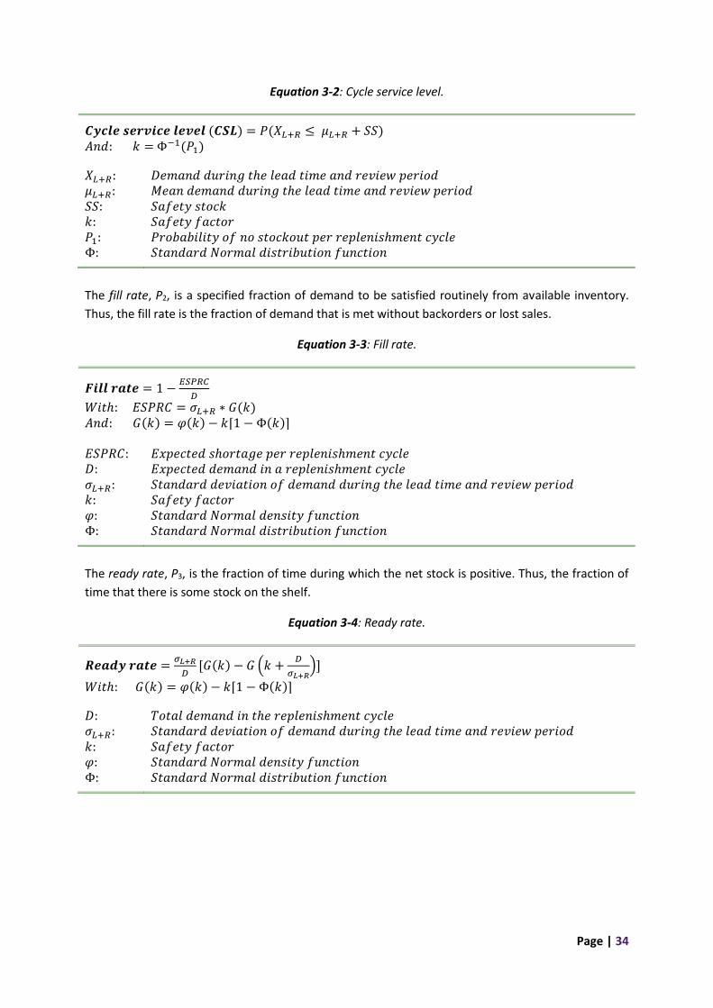
Page | 34
Equation 3-2: Cycle service level.
𝑪𝒚𝒄𝒍𝒆 𝒔𝒆𝒓𝒗𝒊𝒄𝒆 𝒍𝒆𝒗𝒆𝒍 (𝑪𝑺𝑳) = 𝑃(𝑋𝐿+𝑅 ≤ 𝜇𝐿+𝑅 + 𝑆𝑆) 𝐴𝑛𝑑: 𝑘 = Φ−1(𝑃1)
𝑋𝐿+𝑅: 𝜇𝐿+𝑅: 𝑆𝑆: 𝑘: 𝑃1: Φ:
𝐷𝑒𝑚𝑎𝑛𝑑 𝑑𝑢𝑟𝑖𝑛𝑔 𝑡ℎ𝑒 𝑙𝑒𝑎𝑑 𝑡𝑖𝑚𝑒 𝑎𝑛𝑑 𝑟𝑒𝑣𝑖𝑒𝑤 𝑝𝑒𝑟𝑖𝑜𝑑 𝑀𝑒𝑎𝑛 𝑑𝑒𝑚𝑎𝑛𝑑 𝑑𝑢𝑟𝑖𝑛𝑔 𝑡ℎ𝑒 𝑙𝑒𝑎𝑑 𝑡𝑖𝑚𝑒 𝑎𝑛𝑑 𝑟𝑒𝑣𝑖𝑒𝑤 𝑝𝑒𝑟𝑖𝑜𝑑 𝑆𝑎𝑓𝑒𝑡𝑦 𝑠𝑡𝑜𝑐𝑘 𝑆𝑎𝑓𝑒𝑡𝑦 𝑓𝑎𝑐𝑡𝑜𝑟 𝑃𝑟𝑜𝑏𝑎𝑏𝑖𝑙𝑖𝑡𝑦 𝑜𝑓 𝑛𝑜 𝑠𝑡𝑜𝑐𝑘𝑜𝑢𝑡 𝑝𝑒𝑟 𝑟𝑒𝑝𝑙𝑒𝑛𝑖𝑠ℎ𝑚𝑒𝑛𝑡 𝑐𝑦𝑐𝑙𝑒 𝑆𝑡𝑎𝑛𝑑𝑎𝑟𝑑 𝑁𝑜𝑟𝑚𝑎𝑙 𝑑𝑖𝑠𝑡𝑟𝑖𝑏𝑢𝑡𝑖𝑜𝑛 𝑓𝑢𝑛𝑐𝑡𝑖𝑜𝑛
The fill rate, P2, is a specified fraction of demand to be satisfied routinely from available inventory.
Thus, the fill rate is the fraction of demand that is met without backorders or lost sales.
Equation 3-3: Fill rate.
𝑭𝒊𝒍𝒍 𝒓𝒂𝒕𝒆 = 1 −𝐸𝑆𝑃𝑅𝐶
𝐷
𝑊𝑖𝑡ℎ: 𝐸𝑆𝑃𝑅𝐶 = 𝜎𝐿+𝑅 ∗ 𝐺(𝑘) 𝐴𝑛𝑑: 𝐺(𝑘) = 𝜑(𝑘) − 𝑘[1 − Φ(𝑘)]
𝐸𝑆𝑃𝑅𝐶: 𝐷: 𝜎𝐿+𝑅: 𝑘: 𝜑: Φ:
𝐸𝑥𝑝𝑒𝑐𝑡𝑒𝑑 𝑠ℎ𝑜𝑟𝑡𝑎𝑔𝑒 𝑝𝑒𝑟 𝑟𝑒𝑝𝑙𝑒𝑛𝑖𝑠ℎ𝑚𝑒𝑛𝑡 𝑐𝑦𝑐𝑙𝑒 𝐸𝑥𝑝𝑒𝑐𝑡𝑒𝑑 𝑑𝑒𝑚𝑎𝑛𝑑 𝑖𝑛 𝑎 𝑟𝑒𝑝𝑙𝑒𝑛𝑖𝑠ℎ𝑚𝑒𝑛𝑡 𝑐𝑦𝑐𝑙𝑒 𝑆𝑡𝑎𝑛𝑑𝑎𝑟𝑑 𝑑𝑒𝑣𝑖𝑎𝑡𝑖𝑜𝑛 𝑜𝑓 𝑑𝑒𝑚𝑎𝑛𝑑 𝑑𝑢𝑟𝑖𝑛𝑔 𝑡ℎ𝑒 𝑙𝑒𝑎𝑑 𝑡𝑖𝑚𝑒 𝑎𝑛𝑑 𝑟𝑒𝑣𝑖𝑒𝑤 𝑝𝑒𝑟𝑖𝑜𝑑 𝑆𝑎𝑓𝑒𝑡𝑦 𝑓𝑎𝑐𝑡𝑜𝑟 𝑆𝑡𝑎𝑛𝑑𝑎𝑟𝑑 𝑁𝑜𝑟𝑚𝑎𝑙 𝑑𝑒𝑛𝑠𝑖𝑡𝑦 𝑓𝑢𝑛𝑐𝑡𝑖𝑜𝑛 𝑆𝑡𝑎𝑛𝑑𝑎𝑟𝑑 𝑁𝑜𝑟𝑚𝑎𝑙 𝑑𝑖𝑠𝑡𝑟𝑖𝑏𝑢𝑡𝑖𝑜𝑛 𝑓𝑢𝑛𝑐𝑡𝑖𝑜𝑛
The ready rate, P3, is the fraction of time during which the net stock is positive. Thus, the fraction of
time that there is some stock on the shelf.
Equation 3-4: Ready rate.
𝑹𝒆𝒂𝒅𝒚 𝒓𝒂𝒕𝒆 =𝜎𝐿+𝑅
𝐷[𝐺(𝑘) − 𝐺 (𝑘 +
𝐷
𝜎𝐿+𝑅)]
𝑊𝑖𝑡ℎ: 𝐺(𝑘) = 𝜑(𝑘) − 𝑘[1 − Φ(𝑘)]
𝐷: 𝜎𝐿+𝑅: 𝑘: 𝜑: Φ:
𝑇𝑜𝑡𝑎𝑙 𝑑𝑒𝑚𝑎𝑛𝑑 𝑖𝑛 𝑡ℎ𝑒 𝑟𝑒𝑝𝑙𝑒𝑛𝑖𝑠ℎ𝑚𝑒𝑛𝑡 𝑐𝑦𝑐𝑙𝑒 𝑆𝑡𝑎𝑛𝑑𝑎𝑟𝑑 𝑑𝑒𝑣𝑖𝑎𝑡𝑖𝑜𝑛 𝑜𝑓 𝑑𝑒𝑚𝑎𝑛𝑑 𝑑𝑢𝑟𝑖𝑛𝑔 𝑡ℎ𝑒 𝑙𝑒𝑎𝑑 𝑡𝑖𝑚𝑒 𝑎𝑛𝑑 𝑟𝑒𝑣𝑖𝑒𝑤 𝑝𝑒𝑟𝑖𝑜𝑑 𝑆𝑎𝑓𝑒𝑡𝑦 𝑓𝑎𝑐𝑡𝑜𝑟 𝑆𝑡𝑎𝑛𝑑𝑎𝑟𝑑 𝑁𝑜𝑟𝑚𝑎𝑙 𝑑𝑒𝑛𝑠𝑖𝑡𝑦 𝑓𝑢𝑛𝑐𝑡𝑖𝑜𝑛 𝑆𝑡𝑎𝑛𝑑𝑎𝑟𝑑 𝑁𝑜𝑟𝑚𝑎𝑙 𝑑𝑖𝑠𝑡𝑟𝑖𝑏𝑢𝑡𝑖𝑜𝑛 𝑓𝑢𝑛𝑐𝑡𝑖𝑜𝑛
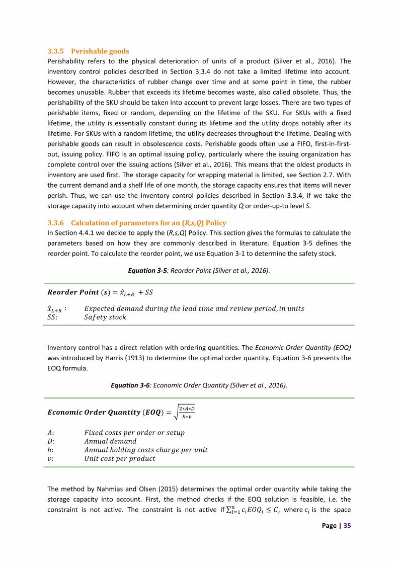
Page | 35
3.3.5 Perishable goods
Perishability refers to the physical deterioration of units of a product (Silver et al., 2016). The
inventory control policies described in Section 3.3.4 do not take a limited lifetime into account.
However, the characteristics of rubber change over time and at some point in time, the rubber
becomes unusable. Rubber that exceeds its lifetime becomes waste, also called obsolete. Thus, the
perishability of the SKU should be taken into account to prevent large losses. There are two types of
perishable items, fixed or random, depending on the lifetime of the SKU. For SKUs with a fixed
lifetime, the utility is essentially constant during its lifetime and the utility drops notably after its
lifetime. For SKUs with a random lifetime, the utility decreases throughout the lifetime. Dealing with
perishable goods can result in obsolescence costs. Perishable goods often use a FIFO, first-in-first-
out, issuing policy. FIFO is an optimal issuing policy, particularly where the issuing organization has
complete control over the issuing actions (Silver et al., 2016). This means that the oldest products in
inventory are used first. The storage capacity for wrapping material is limited, see Section 2.7. With
the current demand and a shelf life of one month, the storage capacity ensures that items will never
perish. Thus, we can use the inventory control policies described in Section 3.3.4, if we take the
storage capacity into account when determining order quantity Q or order-up-to level S.
3.3.6 Calculation of parameters for an (R,s,Q) Policy
In Section 4.4.1 we decide to apply the (R,s,Q) Policy. This section gives the formulas to calculate the
parameters based on how they are commonly described in literature. Equation 3-5 defines the
reorder point. To calculate the reorder point, we use Equation 3-1 to determine the safety stock.
Equation 3-5: Reorder Point (Silver et al., 2016).
𝑹𝒆𝒐𝒓𝒅𝒆𝒓 𝑷𝒐𝒊𝒏𝒕 (𝒔) = 𝑥𝐿+𝑅 + 𝑆𝑆
𝑥𝐿+𝑅 ∶ 𝑆𝑆:
𝐸𝑥𝑝𝑒𝑐𝑡𝑒𝑑 𝑑𝑒𝑚𝑎𝑛𝑑 𝑑𝑢𝑟𝑖𝑛𝑔 𝑡ℎ𝑒 𝑙𝑒𝑎𝑑 𝑡𝑖𝑚𝑒 𝑎𝑛𝑑 𝑟𝑒𝑣𝑖𝑒𝑤 𝑝𝑒𝑟𝑖𝑜𝑑, 𝑖𝑛 𝑢𝑛𝑖𝑡𝑠 𝑆𝑎𝑓𝑒𝑡𝑦 𝑠𝑡𝑜𝑐𝑘
Inventory control has a direct relation with ordering quantities. The Economic Order Quantity (EOQ)
was introduced by Harris (1913) to determine the optimal order quantity. Equation 3-6 presents the
EOQ formula.
Equation 3-6: Economic Order Quantity (Silver et al., 2016).
𝑬𝒄𝒐𝒏𝒐𝒎𝒊𝒄 𝑶𝒓𝒅𝒆𝒓 𝑸𝒖𝒂𝒏𝒕𝒊𝒕𝒚 (𝑬𝑶𝑸) = √2∗𝐴∗𝐷
ℎ∗𝑣
𝐴: 𝐷: ℎ: 𝑣:
𝐹𝑖𝑥𝑒𝑑 𝑐𝑜𝑠𝑡𝑠 𝑝𝑒𝑟 𝑜𝑟𝑑𝑒𝑟 𝑜𝑟 𝑠𝑒𝑡𝑢𝑝 𝐴𝑛𝑛𝑢𝑎𝑙 𝑑𝑒𝑚𝑎𝑛𝑑 𝐴𝑛𝑛𝑢𝑎𝑙 ℎ𝑜𝑙𝑑𝑖𝑛𝑔 𝑐𝑜𝑠𝑡𝑠 𝑐ℎ𝑎𝑟𝑔𝑒 𝑝𝑒𝑟 𝑢𝑛𝑖𝑡 𝑈𝑛𝑖𝑡 𝑐𝑜𝑠𝑡 𝑝𝑒𝑟 𝑝𝑟𝑜𝑑𝑢𝑐𝑡
The method by Nahmias and Olsen (2015) determines the optimal order quantity while taking the
storage capacity into account. First, the method checks if the EOQ solution is feasible, i.e. the
constraint is not active. The constraint is not active if ∑ 𝑐𝑖𝐸𝑂𝑄𝑖𝑛𝑖=1 ≤ 𝐶, where 𝑐𝑖 is the space

Page | 36
consumed by one unit of product i for i=1, 2, .., n and 𝐶 is the total storage space available. If the
constraint is not active, the optimal solution is 𝑄𝑖∗ = 𝐸𝑂𝑄𝑖. If the constraint is active, it means that
the constraint is binding. Thus, the solution without the constraint is different from the solution with
the constraint. The constraint is active if ∑ 𝑐𝑖𝐸𝑂𝑄𝑖𝑛𝑖=1 > 𝐶. If the constraint is active, we reduce the
order quantities. The first step is to compute the ratios 𝑐𝑖
ℎ𝑖𝑣𝑖, where ℎ𝑖 is the annual holding costs
charge per unit of product i for i=1, 2, .., n and 𝑣𝑖 is the unit costs of product i for i=1, 2, .., n. If the
values are indifferent, we calculate the optimal solution with Equation 3-7.
Equation 3-7: Optimal order quantity if the ratios are indifferent
𝑸𝒊∗ = 𝑚𝐸𝑂𝑄𝑖
𝑤ℎ𝑒𝑟𝑒: 𝑚 = 𝐶/[∑ (𝑛𝑖=1 𝑐𝑖𝐸𝑂𝑄𝑖)]
𝑄𝑖∗:
𝐸𝑂𝑄𝑖: 𝐶: 𝑐𝑖:
𝑂𝑝𝑡𝑖𝑚𝑎𝑙 𝑜𝑟𝑑𝑒𝑟 𝑞𝑢𝑎𝑛𝑡𝑖𝑡𝑦 𝑜𝑓 𝑆𝐾𝑈 𝑖 𝐸𝑐𝑜𝑛𝑜𝑚𝑖𝑐 𝑂𝑟𝑑𝑒𝑟 𝑄𝑢𝑎𝑛𝑡𝑖𝑡𝑦 𝑜𝑓 𝑆𝐾𝑈 𝑖 𝑇𝑜𝑡𝑎𝑙 𝑠𝑡𝑜𝑟𝑎𝑔𝑒 𝑐𝑎𝑝𝑎𝑐𝑖𝑡𝑦 𝑆𝑝𝑎𝑐𝑒 𝑐𝑜𝑛𝑠𝑢𝑚𝑒𝑑 𝑏𝑦 𝑜𝑛𝑒 𝑢𝑛𝑖𝑡 𝑜𝑓 𝑝𝑟𝑜𝑑𝑢𝑐𝑡 𝑜𝑓 𝑆𝐾𝑈 𝑖
If the values are different, we calculate the optimal solution with Equation 3-8. The constant 𝜃,
known as the Lagrange multiplier, reduces the lot sizes by increasing the effective holding cost. The
value of 𝜃 can be interpreted as the marginal benefit of an additional square foot of space. The
correct value of 𝜃 can be found by trial and error or by a search technique. Note that 𝜃 > 0, so that
the search can be limited to positive numbers only.
Equation 3-8: Optimal order quantity if the ratios are different
𝑸𝒊∗ = √
2∗𝐴𝑖∗𝐷𝑖
ℎ𝑖𝑣𝑖+2𝜃𝑐𝑖
𝑤ℎ𝑒𝑟𝑒: 𝜃 𝑖𝑠 𝑎 𝑐𝑜𝑛𝑠𝑡𝑎𝑛𝑡 𝑐ℎ𝑜𝑠𝑒𝑛 𝑠𝑜 𝑡ℎ𝑎𝑡 ∑ 𝑐𝑖𝑄𝑖∗𝑛
𝑖=1 = 𝐶
𝑄𝑖∗:
𝐴𝑖: 𝐷𝑖: ℎ𝑖: 𝑣𝑖: 𝑐𝑖: 𝐶:
𝑂𝑝𝑡𝑖𝑚𝑎𝑙 𝑜𝑟𝑑𝑒𝑟 𝑞𝑢𝑎𝑛𝑡𝑖𝑡𝑦 𝑜𝑓 𝑆𝐾𝑈 𝑖 𝐹𝑖𝑥𝑒𝑑 𝑐𝑜𝑠𝑡𝑠 𝑝𝑒𝑟 𝑜𝑟𝑑𝑒𝑟 𝑜𝑟 𝑠𝑒𝑡𝑢𝑝 𝑓𝑜𝑟 𝑆𝐾𝑈 𝑖 𝐴𝑛𝑛𝑢𝑎𝑙 𝑑𝑒𝑚𝑎𝑛𝑑 𝑜𝑓 𝑆𝐾𝑈 𝑖 𝐴𝑛𝑛𝑢𝑎𝑙 ℎ𝑜𝑙𝑑𝑖𝑛𝑔 𝑐𝑜𝑠𝑡𝑠 𝑐ℎ𝑎𝑟𝑔𝑒 𝑝𝑒𝑟 𝑢𝑛𝑖𝑡 𝑜𝑓 𝑆𝐾𝑈 𝑖 𝑈𝑛𝑖𝑡 𝑐𝑜𝑠𝑡 𝑝𝑒𝑟 𝑝𝑟𝑜𝑑𝑢𝑐𝑡 𝑜𝑓 𝑆𝐾𝑈 𝑖 𝑆𝑝𝑎𝑐𝑒 𝑐𝑜𝑛𝑠𝑢𝑚𝑒𝑑 𝑏𝑦 𝑜𝑛𝑒 𝑢𝑛𝑖𝑡 𝑜𝑓 𝑝𝑟𝑜𝑑𝑢𝑐𝑡 𝑜𝑓 𝑆𝐾𝑈 𝑖 𝑇𝑜𝑡𝑎𝑙 𝑠𝑡𝑜𝑟𝑎𝑔𝑒 𝑐𝑎𝑝𝑎𝑐𝑖𝑡𝑦
Finally, with fill rate P2 as service measure (see Section 4.4.1), we use Equation 3-9 to calculate k.
Equation 3-9: Safety factor k, given P2 as service measure.
𝑮(𝒌) =𝑄
𝜎𝐿+𝑅(1 − 𝑃2)
𝑘: 𝑆𝑎𝑓𝑒𝑡𝑦 𝑓𝑎𝑐𝑡𝑜𝑟
Page | 37
𝜎𝐿+𝑅: 𝑄: 𝑃2:
𝑆𝑡𝑎𝑛𝑑𝑎𝑟𝑑 𝑑𝑒𝑣𝑖𝑎𝑡𝑖𝑜𝑛 𝑜𝑓 𝑑𝑒𝑚𝑎𝑛𝑑 𝑑𝑢𝑟𝑖𝑛𝑔 𝑡ℎ𝑒 𝑙𝑒𝑎𝑑 𝑡𝑖𝑚𝑒 𝑎𝑛𝑑 𝑟𝑒𝑣𝑖𝑒𝑤 𝑝𝑒𝑟𝑖𝑜𝑑 𝑂𝑟𝑑𝑒𝑟 𝑞𝑢𝑎𝑛𝑡𝑖𝑡𝑦 𝐹𝑟𝑎𝑐𝑡𝑖𝑜𝑛 𝑜𝑓 𝑑𝑒𝑚𝑎𝑛𝑑 𝑠𝑎𝑡𝑖𝑠𝑓𝑖𝑒𝑑 𝑑𝑖𝑟𝑒𝑐𝑡𝑙𝑦 𝑓𝑟𝑜𝑚 𝑠ℎ𝑒𝑙𝑓
3.3 Conclusion In this chapter we presented an overview of the necessary theoretical knowledge to tackle our
research problems. We focused on the subjects operations management philosophies, bottleneck
identification methods, and inventory control.
In Section 3.1 we discussed the most common operations management philosophies to improve the
manufacturing performance. The operations management philosophies that are included are total
quality management, business process re-engineering, lean manufacturing, theory of constraints,
and six sigma. We finished this section with a discussion on the differences between the
philosophies.
In Section 3.2 we described several bottleneck identification methods and summarized the methods
with a table containing the characteristics of each method. The bottleneck identification methods
that are included are the process time method, utilization method, inventory based methods, arrow
method, turning point method, active period method, bottleneck walk, and simulation based
methods.
In Section 3.3 we discussed various aspects of inventory control. The main two reasons for having
stock are economies of scale and uncertainties. We elaborated on the categorization of uncertainty
types, the classification of SKUs, and the advantages and disadvantages of periodic and continuous
review. We discussed the five inventory control policies described by Silver et al. (2016) and Janssen
et al. (1996). These inventory control policies are the (s,Q), (s,S), (R,S), (R,s,S), and (R,s,Q) policy.
Furthermore, we mentioned the different cost and service objectives and provided formulas for the
service objectives. Finally, we discussed the influence of perishable goods on inventory control and
we provided formulas to calculate the parameters of a (R,s,Q) policy.

Page | 38

Page | 39
4. Model framework This chapter focuses on the model framework. The framework contains steps 1 to 3 of the TOC cycle
of ongoing improvement. First, Section 4.1 presents the model framework. Second, we explain the
processes within the framework in Sections 4.2 to 4.4. In Section 4.2 we determine the phases for the
bottleneck identification process, which form step 1 of the TOC cycle. In Section 4.3 we introduce the
phase for the optimization of the bottleneck, which forms step 2 of the TOC cycle. In Section 4.3 we
introduce the phases for subordinating the non-bottleneck processes, which form step 3 of the TOC
cycle.
4.1 Model framework flowchart The model framework covers steps 1 to 3 of the TOC cycle of ongoing improvement and consists of
seven phases. Phases 1 to 4 form the bottleneck identification method and are described in Section
4.2. Section 4.3 describes Phase 5, which is part of the bottleneck optimization process. Section 4.4
describes Phases 6 and 7 which form the process to align all non-bottleneck processes to support the
bottleneck process. Figure 4.1 represents the model framework.
Figure 4.1: Model framework.
Page | 40
4.2 Bottleneck identification process In order to develop a bottleneck identification process, we need to know which identification
methods are suitable. First, we discuss the requirements for the bottleneck identification method in
Section 4.2.1. In Section 4.2.2 we decide which bottleneck identification method is suitable and in
Sections 4.2.3 to 4.2.6 we explain the phases of the bottleneck identification process.
4.2.1 Requirements from Apollo Vredestein
There are some requirements for the bottleneck identification method, because it has to fit the
situation at Apollo Vredestein. First of all, the method has to be applicable on complex, parallel
systems as the production at Apollo Vredestein is not serial. Second, Apollo Vredestein has finite
buffers and does not have visible queueing, see Section 3.2.7. Thus, the method should not require
infinite buffers or visibility. Third, Apollo Vredestein has a need to know the historical bottleneck,
because they want to know what changes can be made for long term improvements. Monitoring a
real-time bottleneck can be used for momentary improvements on the operational level. This is
mostly interesting if there is a continuously shifting bottleneck and this is not expected. Also, they
ask for a rather simple method that is understandable and workable for Industrial Engineers within
Apollo Vredestein. With workable we mean that they have to be able to use the method themselves
within a reasonable time frame. Also, they have to be able to alter the method themselves if changes
occur. The last requirement is “use what you got”, meaning that the method can only use data if the
data is available at Apollo Vredestein.
4.2.2 Suitable bottleneck identification method for Apollo Vredestein
Considering all the requirements, the data availability, and the method characteristics from Table
3.1, none of the bottleneck identification methods satisfy all requirements. We do not use the
average waiting time method, active period method and average active period method, because the
required data is not available. The bottleneck walk is not applicable, because we are interested in the
most significant long-term bottleneck, which is a historical bottleneck. Also, we do not use a
simulation based method, because it is not easily altered by others if changes occur, which results in
a low workability. We do not use the process time method, because it can only work with constant
cycle times (which is not the case) and it only indicates the maximum capacity, not the bottleneck.
This results in three remaining methods: the utilization method, arrow method, and turning point
method. All these methods are not designed for the system type. This is why we combine the
principles of two methods and data availability to identify the bottleneck. We use two methods that
are based on (partially) different data, because we want to use the second method as verification.
The arrow method and the turning point method base their result on the same data. Thus, we use
the arrow method or the turning point method in combination with the utilization method. The
turning point method has the advantage that it can also be used on complex serial systems in
comparison with the arrow method. Thus, we use the turning point method.
To improve the result of the methods, we use data availability to filter out machines with limited
data. We define data availability as the amount of available time that is justified in bookings. The
data availability varies among the machines. This is caused by different interests from the
coordinators. Some machines have a very low utilization, which makes their losses uninteresting for
the coordinators. This means that no matter how poor their performance is, they always have
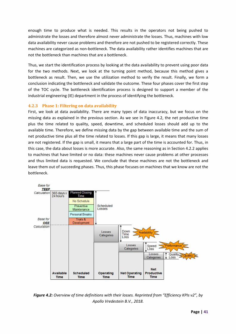
Page | 41
enough time to produce what is needed. This results in the operators not being pushed to
administrate the losses and therefore almost never administrate the losses. Thus, machines with low
data availability never cause problems and therefore are not pushed to be registered correctly. These
machines are categorized as non-bottleneck. The data availability rather identifies machines that are
not the bottleneck than machines that are a bottleneck.
Thus, we start the identification process by looking at the data availability to prevent using poor data
for the two methods. Next, we look at the turning point method, because this method gives a
bottleneck as result. Then, we use the utilization method to verify the result. Finally, we form a
conclusion indicating the bottleneck and validate the outcome. These four phases cover the first step
of the TOC cycle. The bottleneck identification process is designed to support a member of the
industrial engineering (IE) department in the process of identifying the bottleneck.
4.2.3 Phase 1: Filtering on data availability
First, we look at data availability. There are many types of data inaccuracy, but we focus on the
missing data as explained in the previous section. As we see in Figure 4.2, the net productive time
plus the time related to quality, speed, downtime, and scheduled losses should add up to the
available time. Therefore, we define missing data by the gap between available time and the sum of
net productive time plus all the time related to losses. If this gap is large, it means that many losses
are not registered. If the gap is small, it means that a large part of the time is accounted for. Thus, in
this case, the data about losses is more accurate. Also, the same reasoning as in Section 4.2.2 applies
to machines that have limited or no data: these machines never cause problems at other processes
and thus limited data is requested. We conclude that these machines are not the bottleneck and
leave them out of succeeding phases. Thus, this phase focuses on machines that we know are not the
bottleneck.
Figure 4.2: Overview of time definitions with their losses. Reprinted from “Efficiency KPIs v2”, by
Apollo Vredestein B.V., 2018.
Page | 42
In practice the gap also includes the category speed loss. All the losses that occur but have no
explanation and consequentially are not booked, are included as speed losses. Because they are not
booked, they fall into our gap while they should have been categorized as speed losses. The value of
the boundary is not an exact value that can be calculated. Because we rather include non-bottleneck
machines than exclude bottleneck machines, we rather have the boundary too high than too low. In
consultation with a group of employees who have knowledge about the machines and their data, we
set the boundary on 50%. This means that if less than 50% of the time is booked, the machine is
categorized as non-bottleneck. From here on, the gap between available time and the sum of net
productive time plus all the losses is called GAP. The GAP(%) can be calculated using the following
formula: 𝐺𝐴𝑃(%) =𝐴𝑣𝑎𝑖𝑙𝑎𝑏𝑙𝑒 𝑡𝑖𝑚𝑒−𝑙𝑜𝑠𝑠𝑒𝑠−𝑛𝑒𝑡 𝑝𝑟𝑜𝑑𝑢𝑐𝑡𝑖𝑣𝑒 𝑡𝑖𝑚𝑒
𝐴𝑣𝑎𝑖𝑙𝑎𝑏𝑙𝑒 𝑡𝑖𝑚𝑒.
4.2.4 Phase 2: Turning point method
Next, we use the principle of the turning point method. The “turning point” (𝑗) is the station where
the trend changes of blockage being higher than starvation to starvation being higher than blockage.
Resulting in 𝑇𝐵𝑗 + 𝑇𝑆𝑗 (see Section 3.2.5) being the smallest sum in the chain. As we do not have a
serial system, it is not clear what causes the starvation or the blockage by looking at 𝑇𝐵𝑖 and 𝑇𝑆𝑖.
This makes comparing the 𝑇𝐵𝑗 with 𝑇𝑆𝑗+1 not helpful. However, we should still be able to see a
rough pattern starting upstream with positive 𝑇𝐵𝑖 − 𝑇𝑆𝑖, changing into a 𝑇𝐵𝑖 − 𝑇𝑆𝑖 around zero and
ending downstream with a negative 𝑇𝐵𝑖 − 𝑇𝑆𝑖. Using the principle that 𝑇𝐵𝑗 + 𝑇𝑆𝑗 is the smallest sum
in the chain, both 𝑇𝐵𝑗 and 𝑇𝑆𝑗 should be close to zero. Thus, the station with the lowest 𝑇𝐵𝑗 + 𝑇𝑆𝑗 is
the bottleneck in a serial system. This method is designed for serial systems, not parallel systems. As
a result, it does not take the complexity of a parallel system into account. Thus, we do not want to
select the bottleneck immediately. Also, the differences in totals are small for these machines and
the lowest sum can also be caused by losses that are not registered. To prevent selecting the wrong
machine as the bottleneck, we use a boundary to select the machines to be considered as
bottleneck. We cannot calculate an exact value for the boundary, thus we base the boundary on the
data. We take a minimum of three machines to be able to compare them. Furthermore, we include
machines until the difference with the previous machine is more than 1%, up to a maximum of 𝑇𝐵𝑖 +
𝑇𝑆𝑖 = 5%. Following these steps, the boundary is set at 𝑇𝐵𝑖 + 𝑇𝑆𝑖 < 2%, see Table 5.2. This also
indicates that if 𝑇𝐵𝑖 + 𝑇𝑆𝑖 ≥ 2%, we categorize the machine as non-bottleneck.
To select a machine as the most significant bottleneck, we compare the amount of starvation caused
by the machines. This is different to the first part, where we use the amount of starvation at the
machine. Because of the complex system, the first part does not tell us what caused the starvation.
Now, we compare the starvation (in minutes) that the machines have caused for subsequent
processes only for the machines selected to be considered as a bottleneck (𝑇𝐵𝑖 + 𝑇𝑆𝑖 < 2%). We
obtain this information by linking the starvation description at a machine, which describes the
component that is missing, to the preceding machine where the missing component should be
produced, which we obtain from the flowcharts in Appendix 1. We identify the machine that causes
the most minutes of starvation for subsequent processes as the bottleneck. Also, we check if the rest
of the numbers in this figure match the conclusion from the first part of Phase 2.
4.2.5 Phase 3: Utilization method
Next, we use the utilization method to verify the turning point method (see Section 3.2.2). We define
the utilization as the percentage of time a resource is active (Roser et al., 2003). We choose this
definition, because it includes the influence of losses such as breakdown and repair time in the
Page | 43
calculation. The result is that machines can be identified as the bottleneck if they produce a small
part of the time because of high losses.
An active state is that state of the machine when the machine produces a part or is being serviced or
setup, whereas the inactive state of the machine is when the machine is waiting for the part or
waiting to be serviced or waiting for the removal of the parts from the machine (Roser et al., 2003).
Using the utilization method, the bottleneck is identified by looking at the gap between active time
and total time. The smaller the gap, the higher the utilization. The active time includes performance
losses and as we mentioned before, performance losses are usually not booked and fall in the GAP.
This means that with the data we have, if the performance losses increase, the active time decreases
and the utilization decreases, which is not accurate. Thus, we use the inactive time, rather than the
active time. The utilization is defined as:
𝑈𝑡𝑖𝑙𝑖𝑧𝑎𝑡𝑖𝑜𝑛 =𝐴𝑐𝑡𝑖𝑣𝑒 𝑡𝑖𝑚𝑒
𝐴𝑣𝑎𝑖𝑙𝑎𝑏𝑙𝑒 𝑡𝑖𝑚𝑒=
𝐴𝑣𝑎𝑖𝑙𝑎𝑏𝑙𝑒 𝑡𝑖𝑚𝑒 − 𝐼𝑛𝑎𝑐𝑡𝑖𝑣𝑒 𝑡𝑖𝑚𝑒
𝐴𝑣𝑎𝑖𝑙𝑎𝑏𝑙𝑒 𝑡𝑖𝑚𝑒
Here, the inactive time consists of three inactive states. These are waiting for parts, waiting for
service and blocked. The available time is fixed and equals 480 minutes per machine per shift. The
machine with the largest utilization is considered to be the most significant bottleneck.
4.2.6 Phase 4: Conclusion and validation
Finally, we conclude on the location of the bottleneck and validate our conclusion. This section
elaborates on the conclusion and validation.
Conclusion
We compare the outcomes of the previous phases to determine the location of the bottleneck. Phase
1 only filters and thus does not give an outcome on the location of the bottleneck. If (almost) all
machines are filtered out, we should improve the data first. Otherwise, we compare the outcomes of
Phases 2 and 3. If Phases 2 and 3 result in the same machine, we conclude that that machine is the
bottleneck. If Phases 2 and 3 give a different outcome, we relate this to the principles of the
methods. If the machine has a low utilization, but causes a lot of starvation in succeeding processes,
it is likely that there is a supporting process limiting this machine. If 1 − 𝑢𝑡𝑖𝑙𝑖𝑧𝑎𝑡𝑖𝑜𝑛 is higher than
the blockage and starvation times, it is likely that the machine is waiting for material handling
equipment (MHE) or waiting because of planned breaks for employees that are not substituted. Once
we know the origin of the difference, we decide which machine is the most significant bottleneck, or
if we should improve both because the capacities are balanced.
Validation
To validate the outcome, we use two additional factors:
1. Knowledge of the daily state of affairs
2. Data reliability
First, we take the knowledge of the daily state of affairs into account. The bottleneck identification
process is designed to support a member of the IE department in the process of identifying the
bottleneck. A member of the IE department has good understanding of the system and receives a lot
of information on weak and strong points within production. This results in available knowledge of
the daily state of affairs.
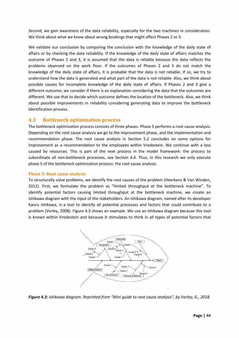
Page | 44
Second, we gain awareness of the data reliability, especially for the two machines in consideration.
We think about what we know about wrong bookings that might affect Phases 2 or 3.
We validate our conclusion by comparing the conclusion with the knowledge of the daily state of
affairs or by checking the data reliability. If the knowledge of the daily state of affairs matches the
outcome of Phases 2 and 3, it is assumed that the data is reliable because the data reflects the
problems observed on the work floor. If the outcomes of Phases 2 and 3 do not match the
knowledge of the daily state of affairs, it is probable that the data is not reliable. If so, we try to
understand how the data is generated and what part of the data is not reliable. Also, we think about
possible causes for incomplete knowledge of the daily state of affairs. If Phases 2 and 3 give a
different outcome, we consider if there is an explanation considering the data that the outcomes are
different. We use that to decide which outcome defines the location of the bottleneck. Also, we think
about possible improvements in reliability considering generating data to improve the bottleneck
identification process.
4.3 Bottleneck optimization process The bottleneck optimization process consists of three phases. Phase 5 performs a root cause analysis.
Depending on the root cause analysis we go to the improvement phase, and the implementation and
recommendation phase. The root cause analysis in Section 5.2 concludes on some options for
improvement as a recommendation to the employees within Vredestein. We continue with a loss
caused by resources. This is part of the next process in the model framework: the process to
subordinate all non-bottleneck processes, see Section 4.4. Thus, in this research we only execute
phase 5 of the bottleneck optimization process: the root cause analysis.
Phase 5: Root cause analysis
To structurally solve problems, we identify the root causes of the problem (Heerkens & Van Winden,
2012). First, we formulate the problem as “limited throughput at the bottleneck machine”. To
identify potential factors causing limited throughput at the bottleneck machine, we create an
Ishikawa diagram with the input of the stakeholders. An Ishikawa diagram, named after its developer
Kaoru Ishikawa, is a tool to identify all potential processes and factors that could contribute to a
problem (Vorley, 2008). Figure 4.3 shows an example. We use an Ishikawa diagram because this tool
is known within Vredestein and because it stimulates to think in all types of potential factors that
Figure 4.3: Ishikawa diagram. Reprinted from “Mini guide to root cause analysis”, by Vorley, G., 2018.
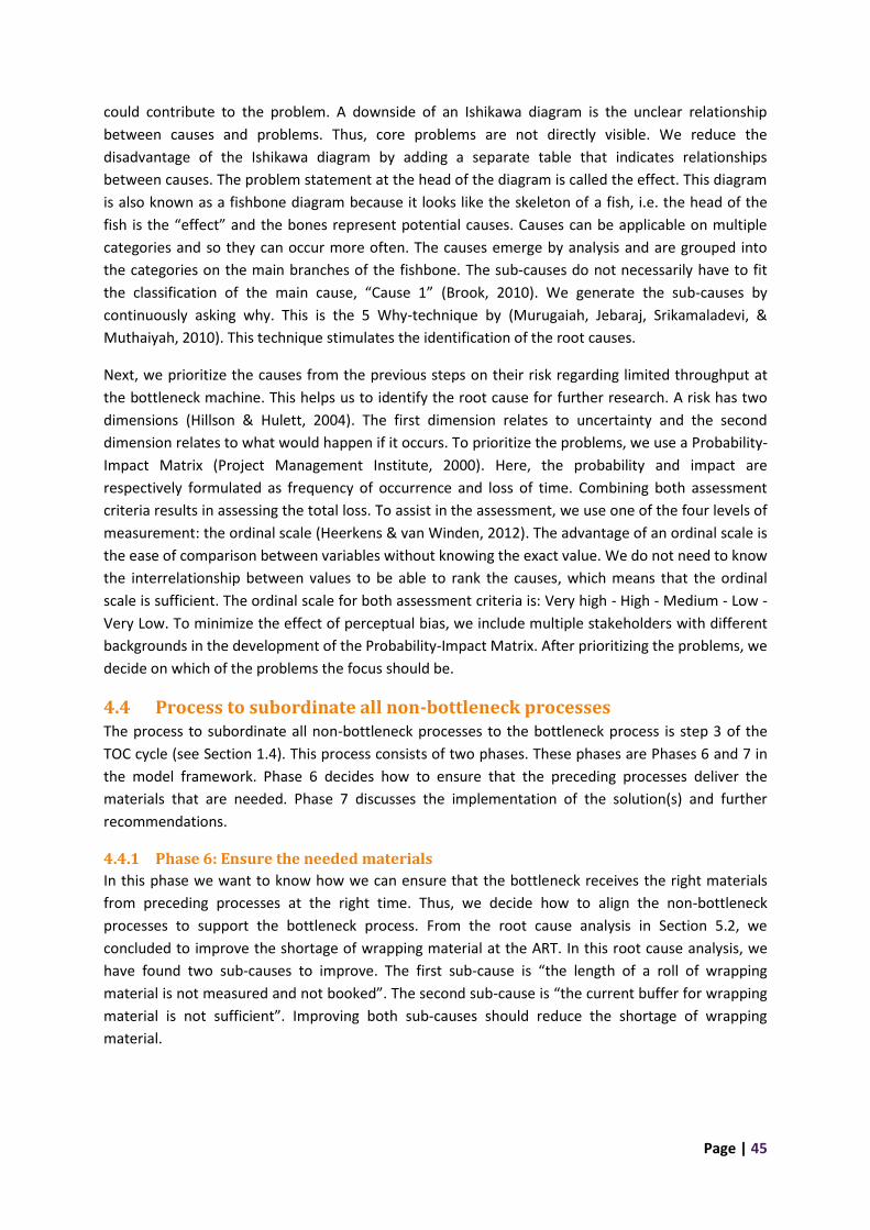
Page | 45
could contribute to the problem. A downside of an Ishikawa diagram is the unclear relationship
between causes and problems. Thus, core problems are not directly visible. We reduce the
disadvantage of the Ishikawa diagram by adding a separate table that indicates relationships
between causes. The problem statement at the head of the diagram is called the effect. This diagram
is also known as a fishbone diagram because it looks like the skeleton of a fish, i.e. the head of the
fish is the “effect” and the bones represent potential causes. Causes can be applicable on multiple
categories and so they can occur more often. The causes emerge by analysis and are grouped into
the categories on the main branches of the fishbone. The sub-causes do not necessarily have to fit
the classification of the main cause, “Cause 1” (Brook, 2010). We generate the sub-causes by
continuously asking why. This is the 5 Why-technique by (Murugaiah, Jebaraj, Srikamaladevi, &
Muthaiyah, 2010). This technique stimulates the identification of the root causes.
Next, we prioritize the causes from the previous steps on their risk regarding limited throughput at
the bottleneck machine. This helps us to identify the root cause for further research. A risk has two
dimensions (Hillson & Hulett, 2004). The first dimension relates to uncertainty and the second
dimension relates to what would happen if it occurs. To prioritize the problems, we use a Probability-
Impact Matrix (Project Management Institute, 2000). Here, the probability and impact are
respectively formulated as frequency of occurrence and loss of time. Combining both assessment
criteria results in assessing the total loss. To assist in the assessment, we use one of the four levels of
measurement: the ordinal scale (Heerkens & van Winden, 2012). The advantage of an ordinal scale is
the ease of comparison between variables without knowing the exact value. We do not need to know
the interrelationship between values to be able to rank the causes, which means that the ordinal
scale is sufficient. The ordinal scale for both assessment criteria is: Very high - High - Medium - Low -
Very Low. To minimize the effect of perceptual bias, we include multiple stakeholders with different
backgrounds in the development of the Probability-Impact Matrix. After prioritizing the problems, we
decide on which of the problems the focus should be.
4.4 Process to subordinate all non-bottleneck processes The process to subordinate all non-bottleneck processes to the bottleneck process is step 3 of the
TOC cycle (see Section 1.4). This process consists of two phases. These phases are Phases 6 and 7 in
the model framework. Phase 6 decides how to ensure that the preceding processes deliver the
materials that are needed. Phase 7 discusses the implementation of the solution(s) and further
recommendations.
4.4.1 Phase 6: Ensure the needed materials
In this phase we want to know how we can ensure that the bottleneck receives the right materials
from preceding processes at the right time. Thus, we decide how to align the non-bottleneck
processes to support the bottleneck process. From the root cause analysis in Section 5.2, we
concluded to improve the shortage of wrapping material at the ART. In this root cause analysis, we
have found two sub-causes to improve. The first sub-cause is “the length of a roll of wrapping
material is not measured and not booked”. The second sub-cause is “the current buffer for wrapping
material is not sufficient”. Improving both sub-causes should reduce the shortage of wrapping
material.
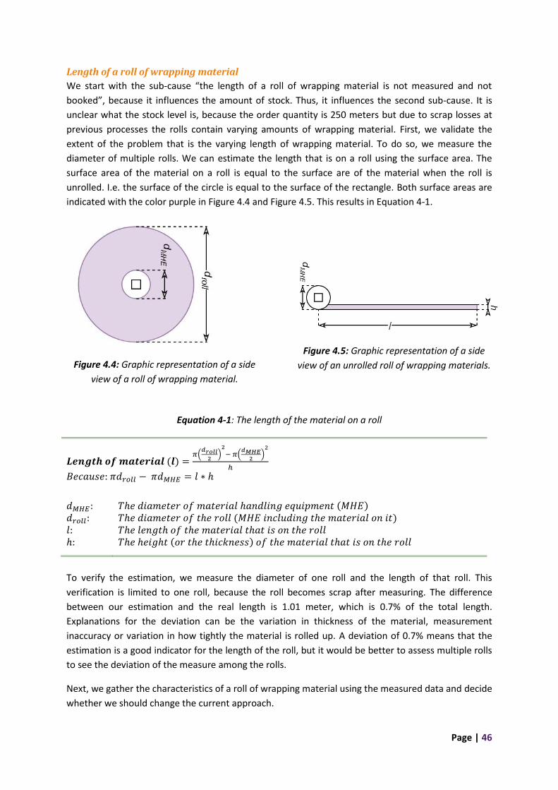
Page | 46
Length of a roll of wrapping material
We start with the sub-cause “the length of a roll of wrapping material is not measured and not
booked”, because it influences the amount of stock. Thus, it influences the second sub-cause. It is
unclear what the stock level is, because the order quantity is 250 meters but due to scrap losses at
previous processes the rolls contain varying amounts of wrapping material. First, we validate the
extent of the problem that is the varying length of wrapping material. To do so, we measure the
diameter of multiple rolls. We can estimate the length that is on a roll using the surface area. The
surface area of the material on a roll is equal to the surface are of the material when the roll is
unrolled. I.e. the surface of the circle is equal to the surface of the rectangle. Both surface areas are
indicated with the color purple in Figure 4.4 and Figure 4.5. This results in Equation 4-1.
Figure 4.4: Graphic representation of a side
view of a roll of wrapping material.
Figure 4.5: Graphic representation of a side
view of an unrolled roll of wrapping materials.
Equation 4-1: The length of the material on a roll
𝑳𝒆𝒏𝒈𝒕𝒉 𝒐𝒇 𝒎𝒂𝒕𝒆𝒓𝒊𝒂𝒍 (𝒍) =𝜋(
𝑑𝑟𝑜𝑙𝑙2
)2
− 𝜋(𝑑𝑀𝐻𝐸
2)
2
ℎ
𝐵𝑒𝑐𝑎𝑢𝑠𝑒: 𝜋𝑑𝑟𝑜𝑙𝑙 − 𝜋𝑑𝑀𝐻𝐸 = 𝑙 ∗ ℎ
𝑑𝑀𝐻𝐸: 𝑑𝑟𝑜𝑙𝑙: 𝑙: ℎ:
𝑇ℎ𝑒 𝑑𝑖𝑎𝑚𝑒𝑡𝑒𝑟 𝑜𝑓 𝑚𝑎𝑡𝑒𝑟𝑖𝑎𝑙 ℎ𝑎𝑛𝑑𝑙𝑖𝑛𝑔 𝑒𝑞𝑢𝑖𝑝𝑚𝑒𝑛𝑡 (𝑀𝐻𝐸) 𝑇ℎ𝑒 𝑑𝑖𝑎𝑚𝑒𝑡𝑒𝑟 𝑜𝑓 𝑡ℎ𝑒 𝑟𝑜𝑙𝑙 (𝑀𝐻𝐸 𝑖𝑛𝑐𝑙𝑢𝑑𝑖𝑛𝑔 𝑡ℎ𝑒 𝑚𝑎𝑡𝑒𝑟𝑖𝑎𝑙 𝑜𝑛 𝑖𝑡) 𝑇ℎ𝑒 𝑙𝑒𝑛𝑔𝑡ℎ 𝑜𝑓 𝑡ℎ𝑒 𝑚𝑎𝑡𝑒𝑟𝑖𝑎𝑙 𝑡ℎ𝑎𝑡 𝑖𝑠 𝑜𝑛 𝑡ℎ𝑒 𝑟𝑜𝑙𝑙 𝑇ℎ𝑒 ℎ𝑒𝑖𝑔ℎ𝑡 (𝑜𝑟 𝑡ℎ𝑒 𝑡ℎ𝑖𝑐𝑘𝑛𝑒𝑠𝑠) 𝑜𝑓 𝑡ℎ𝑒 𝑚𝑎𝑡𝑒𝑟𝑖𝑎𝑙 𝑡ℎ𝑎𝑡 𝑖𝑠 𝑜𝑛 𝑡ℎ𝑒 𝑟𝑜𝑙𝑙
To verify the estimation, we measure the diameter of one roll and the length of that roll. This
verification is limited to one roll, because the roll becomes scrap after measuring. The difference
between our estimation and the real length is 1.01 meter, which is 0.7% of the total length.
Explanations for the deviation can be the variation in thickness of the material, measurement
inaccuracy or variation in how tightly the material is rolled up. A deviation of 0.7% means that the
estimation is a good indicator for the length of the roll, but it would be better to assess multiple rolls
to see the deviation of the measure among the rolls.
Next, we gather the characteristics of a roll of wrapping material using the measured data and decide
whether we should change the current approach.

Page | 47
Inventory control for wrapping material
Next, we continue with the sub-cause “the current buffer for wrapping material is not sufficient”. We
deal with fluctuations or uncertainties, and the current buffer is not sufficient enough to compensate
this, resulting in a shortage of material. To reduce the shortage of material, we set up a new
inventory control policy. The purpose of inventory control policies is to determine when and how
much to order, as well as how to maintain appropriate stock levels to avoid shortages. In this case,
the reason for having stock is uncertainties. We deal with both types of process uncertainty: internal
supply and internal demand uncertainty (see Section 3.3.1). The biggest influence on internal supply
uncertainty is queue waiting time and on internal demand uncertainty is scrap. We take these two
types of uncertainty into account to determine appropriate stock levels. The varying length of a roll
of wrapping material and the number of rolls that are cut from half a calendar roll are uncertainties
caused by scrap. Scrap is a quantity uncertainty and queue waiting time a timing uncertainty. There
are opposite opinions in literature on how to include quantity and timing uncertainty, see Section
3.3.1. We decide to use safety stock for both types of uncertainty, because the safety lead time is
used as a general measure within the company (see Section 2.7). To keep a clear distinction between
machine specific and general buffers, we use safety stock for uncertainty caused by scrap and queue
waiting time. This new inventory control policy will consist of the original safety lead time of two
hours and a yet to be defined safety stock. In the current situation the safety lead time of two hours
buffers for all uncertainties and this is not sufficient. The proposed policy includes a safety stock for
queue waiting time and scrap uncertainty and a two-hour safety lead time for the other remaining
uncertainties that occur. This means that the safety stock and performance regarding the queue
waiting time and scrap uncertainty do not take the safety lead time and other uncertainties into
account.
To set up inventory control for wrapping material we answer the four questions to systematically
establish inventory policies (Silver, Pyke, & Thomas, 2016):
1. How important is the item?
2. Can, or should, the stock status be reviewed continuously or periodically?
3. What form should the inventory policy take?
4. What specific cost or service objectives should be set?
First, we decide on the importance of an item. We look at a small part of the entire system and
define an inventory control policy for two SKUs. The common classification methods, mentioned in
Section 3.3.2, rank the SKUs based on some criteria. In this case, a ranking does not give the desired
results because we only have two SKUs. Using a ranking we can state that one SKU is more important
than the other, but we cannot state that both are important or unimportant. Because of this, we do
not make a classification based on a ranking, such as the percentage of total annual dollar usage.
Both SKUs are input material for the bottleneck and, as we recall from Section 1.4, the throughput of
the system is determined by the throughput of the bottleneck. Thus, a stockout at the bottleneck is a
loss of the entire system. This means both SKUs have a high criticality and we therefore classify them
as A items (see Section 3.3.2).
Second, we choose between a continuous or periodic review period. Vredestein updates their
planning after every shift of 8 hours. Within these 8 hours, the demand does not change. The semi-
finished products needed to build the greentyres must be present two hours before the order starts

Page | 48
at the building machine. Thus, revising the planning of the building department does directly
influence the planning of the semi-finished products. Because the current production planning is
based on a periodic review, we choose to also periodically review the stock level. To minimize the
uncertainty of the stock level we choose a periodic review with review period R equal to one shift of
8 hours. Thus, the demand is set per 8 hours and the stock is reviewed every 8 hours. The advantage
is a lower safety stock compared to a longer review period. This is desired because the space for the
stock of wrapping material is limited. Also, we are dealing with perishable goods. The wrapping
material has a shelf life up to one month. If the material is older than one month, it has to be
disposed of. This is another reason to strive for low safety stocks.
Third, we choose an inventory control policy. The wrapping material has a fixed order quantity (see
Section 2.7). From Table 3.2 in Section 3.3.4 we see that the (R,s,Q) policy is a periodic review policy
and uses a fixed order quantity Q. The advantage of the (R,s,Q) policy is that we can order a multiple
of Q. This means that the policy is able to raise the inventory above the reorder point s if individual
transactions are large. The storage capacity for wrapping material is limited, which ensures that
items will never perish. Thus, we can use the (R,s,Q) policy if we use the method described by
Nahmias and Olsen (2015) to take the storage capacity into account when determining order
quantity Q.
Fourth and last, we decide on the cost or service objective. The goal is to serve the customer, the
ART. It is the bottleneck machine and therefore a high service level is required. Thus, we choose the
method “customer service” to define the safety stock. Another option is the minimizing cost method.
The shortage costs of a bottleneck machine are high, which also results in a high desired service level.
Nevertheless, we choose the customer service method, because the shortage costs are difficult to
define. We can calculate the costs related to the production of a tyre that is asked but not made, but
we do not know the intangible costs, such as reputation damage. The service level is determined by
the company, based on their vision of what is acceptable or desired. Within the customer service
method, there are three common measures: cycle service level, fill rate and ready rate (see Section
3.3.5). Because the time of the bottleneck machine is valuable, the amount of shortage and not the
number of stockout occasions has a large influence on the shortage costs. Every minute that is lost
on the bottleneck machine, could have been used to produce more beads and fulfil a part of the
demand. This means that the longer the stockout, the larger the fraction of demand that is not
satisfied. Thus, we use the fill rate as service measure because the duration of a stockout is taken
into account.
Performance of inventory control
We measure the performance of inventory control by the fill rate, the expected shortage, the
average stock level and the cost of inventory. We calculate the fill rate with and derive the expected
shortage from Equation 3-3. We calculate the cost of inventory using Equation 4-2 and derive the
average stock level from Equation 4-2. The cost of inventory includes ordering cost and holding or
carrying cost. We do not include obsolescence cost, because the storage capacity ensures items will
never perish.
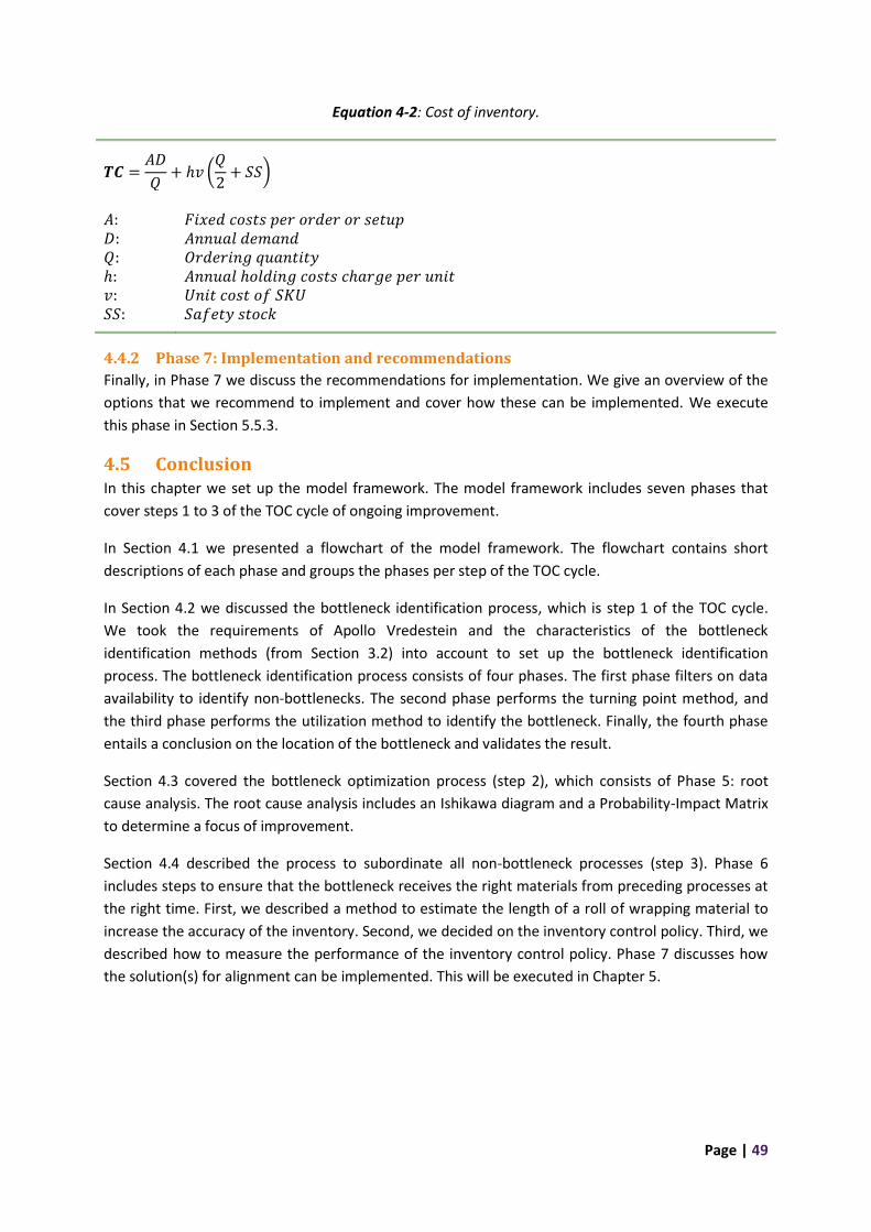
Page | 49
Equation 4-2: Cost of inventory.
𝑻𝑪 =𝐴𝐷
𝑄+ ℎ𝑣 (
𝑄
2+ 𝑆𝑆)
𝐴: 𝐷: 𝑄: ℎ: 𝑣: 𝑆𝑆:
𝐹𝑖𝑥𝑒𝑑 𝑐𝑜𝑠𝑡𝑠 𝑝𝑒𝑟 𝑜𝑟𝑑𝑒𝑟 𝑜𝑟 𝑠𝑒𝑡𝑢𝑝 𝐴𝑛𝑛𝑢𝑎𝑙 𝑑𝑒𝑚𝑎𝑛𝑑 𝑂𝑟𝑑𝑒𝑟𝑖𝑛𝑔 𝑞𝑢𝑎𝑛𝑡𝑖𝑡𝑦 𝐴𝑛𝑛𝑢𝑎𝑙 ℎ𝑜𝑙𝑑𝑖𝑛𝑔 𝑐𝑜𝑠𝑡𝑠 𝑐ℎ𝑎𝑟𝑔𝑒 𝑝𝑒𝑟 𝑢𝑛𝑖𝑡 𝑈𝑛𝑖𝑡 𝑐𝑜𝑠𝑡 𝑜𝑓 𝑆𝐾𝑈 𝑆𝑎𝑓𝑒𝑡𝑦 𝑠𝑡𝑜𝑐𝑘
4.4.2 Phase 7: Implementation and recommendations
Finally, in Phase 7 we discuss the recommendations for implementation. We give an overview of the
options that we recommend to implement and cover how these can be implemented. We execute
this phase in Section 5.5.3.
4.5 Conclusion In this chapter we set up the model framework. The model framework includes seven phases that
cover steps 1 to 3 of the TOC cycle of ongoing improvement.
In Section 4.1 we presented a flowchart of the model framework. The flowchart contains short
descriptions of each phase and groups the phases per step of the TOC cycle.
In Section 4.2 we discussed the bottleneck identification process, which is step 1 of the TOC cycle.
We took the requirements of Apollo Vredestein and the characteristics of the bottleneck
identification methods (from Section 3.2) into account to set up the bottleneck identification
process. The bottleneck identification process consists of four phases. The first phase filters on data
availability to identify non-bottlenecks. The second phase performs the turning point method, and
the third phase performs the utilization method to identify the bottleneck. Finally, the fourth phase
entails a conclusion on the location of the bottleneck and validates the result.
Section 4.3 covered the bottleneck optimization process (step 2), which consists of Phase 5: root
cause analysis. The root cause analysis includes an Ishikawa diagram and a Probability-Impact Matrix
to determine a focus of improvement.
Section 4.4 described the process to subordinate all non-bottleneck processes (step 3). Phase 6
includes steps to ensure that the bottleneck receives the right materials from preceding processes at
the right time. First, we described a method to estimate the length of a roll of wrapping material to
increase the accuracy of the inventory. Second, we decided on the inventory control policy. Third, we
described how to measure the performance of the inventory control policy. Phase 7 discusses how
the solution(s) for alignment can be implemented. This will be executed in Chapter 5.

Page | 50

Page | 51
5. Model implementation In this chapter we execute the phases of the model framework. First, in Section 5.1 we go through
Phases 1 to 4 of the bottleneck identification process. Second, in Section 5.2 we execute Phase 5 of
the bottleneck optimization process. Third, in Section 5.3 we execute the Phases 6 and 7 of the
process to subordinate all non-bottleneck processes.
5.1 Bottleneck identification In this section we execute the four phases of the bottleneck identification process. All the data that
we use for the identification of the bottleneck is from the period 14/1/2019-31/3/2019. The period
length is based on the most recent data available at the start of the phase while excluding the
Christmas holiday during which there is no regular production.
To visualize the principles and provide the information that is needed to perform the phases, we
build a dashboard in Power BI. Power BI is a business analytics solution that visualizes the data and
shares insights across the corresponding organization. We choose to use Power BI because this has
recently been purchased by Apollo Vredestein and is seen as the future of sharing data information
for their organization. The dashboard shows the information for the phases and also some of the
outcomes. Further information about the dashboard can be found in Appendix 2. Below, we
elaborate on the execution of Phases 1 to 4 using the dashboard.
We start with Phase 1: filtering on data availability. Table 5.1 presents the machines with their
GAP(%). All machines with a GAP larger than 50% are not the bottleneck, see Section 4.2.3. From the
table we conclude that FSW4, HLNLB, 96, 97, 98, 99, 27, and 29 are not the bottleneck. For KAL3
there is missing data on the net productive time, which results in the large GAP. The net productive
time is data generated by the system and does not need to be booked. This means that the data is
missing due to a program error. Thus, KAL3 is an exception and is included in the next phases. Also,
there are four machines: Pugno, HVS2, Calemard, and Paint Cabine that have no data and as a result
are not present in the table. Here, we apply the same reasoning as in Section 4.2.2: these machines
rarely cause problems at other processes and therefore no data is requested. Thus, we conclude that
these four machines are also not the bottleneck. In total, Phase 1 leads to the conclusion that FSW4,
HLNLB, 96, 97, 98, 99, Pugno, HVS2, Calemard, and Paint Cabine are not the bottleneck. The
remaining machines are identified as possible bottlenecks.
Table 5.1: GAP (%) per machine.
Machine GAP (%)
FSW4 94.08% ORION 25.40% 9 9.57%
HLNLB 85.68% ART 18.55% 49 9.47%
97 77.12% TRIPL 14.56% 47 9.45%
29 75.78% KAL4 13.98% Agri Press 9.30%
98 73.90% M4 13.75% LTM 7.97%
KAL3 73.79% M5 13.02% 7 7.78%
99 72.94% 11 12.85% 55 7.57%
96 67.23% M6 11.42% M8 7.11%
27 53.34% TINCH 11.25% 53 6.50%
BIAS5 41.84% 43 11.24% 51 0.29%
BIAS7 35.35% 41 10.09%
PASM1 35.08% 45 10.09%
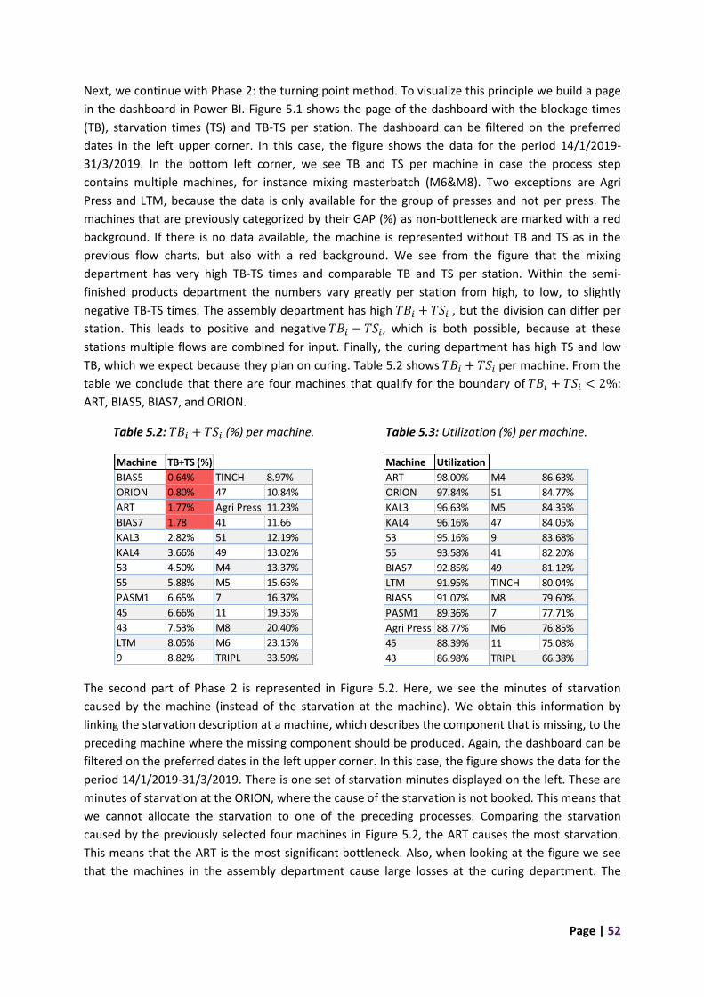
Page | 52
Next, we continue with Phase 2: the turning point method. To visualize this principle we build a page
in the dashboard in Power BI. Figure 5.1 shows the page of the dashboard with the blockage times
(TB), starvation times (TS) and TB-TS per station. The dashboard can be filtered on the preferred
dates in the left upper corner. In this case, the figure shows the data for the period 14/1/2019-
31/3/2019. In the bottom left corner, we see TB and TS per machine in case the process step
contains multiple machines, for instance mixing masterbatch (M6&M8). Two exceptions are Agri
Press and LTM, because the data is only available for the group of presses and not per press. The
machines that are previously categorized by their GAP (%) as non-bottleneck are marked with a red
background. If there is no data available, the machine is represented without TB and TS as in the
previous flow charts, but also with a red background. We see from the figure that the mixing
department has very high TB-TS times and comparable TB and TS per station. Within the semi-
finished products department the numbers vary greatly per station from high, to low, to slightly
negative TB-TS times. The assembly department has high 𝑇𝐵𝑖 + 𝑇𝑆𝑖 , but the division can differ per
station. This leads to positive and negative 𝑇𝐵𝑖 − 𝑇𝑆𝑖, which is both possible, because at these
stations multiple flows are combined for input. Finally, the curing department has high TS and low
TB, which we expect because they plan on curing. Table 5.2 shows 𝑇𝐵𝑖 + 𝑇𝑆𝑖 per machine. From the
table we conclude that there are four machines that qualify for the boundary of 𝑇𝐵𝑖 + 𝑇𝑆𝑖 < 2%:
ART, BIAS5, BIAS7, and ORION.
Table 5.2: 𝑇𝐵𝑖 + 𝑇𝑆𝑖 (%) per machine.
Table 5.3: Utilization (%) per machine.
The second part of Phase 2 is represented in Figure 5.2. Here, we see the minutes of starvation
caused by the machine (instead of the starvation at the machine). We obtain this information by
linking the starvation description at a machine, which describes the component that is missing, to the
preceding machine where the missing component should be produced. Again, the dashboard can be
filtered on the preferred dates in the left upper corner. In this case, the figure shows the data for the
period 14/1/2019-31/3/2019. There is one set of starvation minutes displayed on the left. These are
minutes of starvation at the ORION, where the cause of the starvation is not booked. This means that
we cannot allocate the starvation to one of the preceding processes. Comparing the starvation
caused by the previously selected four machines in Figure 5.2, the ART causes the most starvation.
This means that the ART is the most significant bottleneck. Also, when looking at the figure we see
that the machines in the assembly department cause large losses at the curing department. The
Machine TB+TS (%)
BIAS5 0.64% TINCH 8.97%
ORION 0.80% 47 10.84%
ART 1.77% Agri Press 11.23%
BIAS7 1.78 41 11.66
KAL3 2.82% 51 12.19%
KAL4 3.66% 49 13.02%
53 4.50% M4 13.37%
55 5.88% M5 15.65%
PASM1 6.65% 7 16.37%
45 6.66% 11 19.35%
43 7.53% M8 20.40%
LTM 8.05% M6 23.15%
9 8.82% TRIPL 33.59%
Machine Utilization
ART 98.00% M4 86.63%
ORION 97.84% 51 84.77%
KAL3 96.63% M5 84.35%
KAL4 96.16% 47 84.05%
53 95.16% 9 83.68%
55 93.58% 41 82.20%
BIAS7 92.85% 49 81.12%
LTM 91.95% TINCH 80.04%
BIAS5 91.07% M8 79.60%
PASM1 89.36% 7 77.71%
Agri Press 88.77% M6 76.85%
45 88.39% 11 75.08%
43 86.98% TRIPL 66.38%
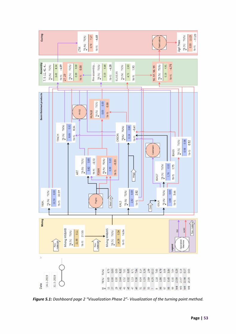
Page | 53
Figure 5.1: Dashboard page 2 “Visualization Phase 2”- Visualization of the turning point method.
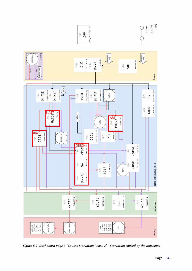
Page | 54
Figure 5.2: Dashboard page 3 “Caused starvation Phase 2” - Starvation caused by the machines .
ART
ORION
BIAS7
BIAS5
Page | 55
largest loss in the assembly department is caused by no beads at the spot of the ART. The starvation
at the ART caused by delivering machines only covers a small part of these losses. This also indicates
that the ART is the most significant bottleneck. Another interesting finding is the starvation at the
assembly department caused by no tread at the spot of the TINCH. This is the second largest loss in
the assembly department, but this machine has plenty of spare time. This research is limited to
managing one bottleneck, thus looking at the TINCH is a recommendation for further research.
Next is Phase 3: utilization method. The utilization method results in Table 5.3. From Table 5.3 we
see that the ART has the highest utilization. This means that the ART is also the most significant
bottleneck when using the utilization method.
The final phase is Phase 4: conclusion and validation. Phases 2 and 3 both indicate that the ART is the
bottleneck. Thus, we conclude that the ART is the bottleneck machine. To validate the outcome, we
discussed the result with the member of the IE department that is responsible for the part of
production that is exclusively for AGRI and SM, and he agreed with it. Because both phases and the
knowledge of the daily state of affairs correspond, we expect the data to be reliable and do not
further investigate the data reliability. Thus, the validation supports the conclusion that the ART is
the most significant bottleneck.
Furthermore, we see from the data that other machines also affect the flow and can be categorized
as secondary bottlenecks. These machines are a recommendation for further research. Below, we
shortly mention our initial findings for those machines. The ORION is a highly utilized machine
causing a small amount of starvation. Because of the high utilization, it is important to keep some
focus on this machine to prevent higher amounts of starvation (at the building department). The
different order between Table 5.2 and Table 5.3 is caused by the inactive state: waiting for service.
The turning point method only takes waiting for service as a consequence of a preceding or
succeeding processes into account, which means blockage and starvation times. However, the
utilization method also considers waiting for service as a consequence of a lack of material handling
equipment or planned breaks for employees that are not substituted. For instance, in Table 5.3 BIAS5
and BIAS7 went down in ranking compared to Table 5.2, which means that the time those machines
wait for service that is not caused by a preceding or succeeding process is high. I.e. there is either a
lack of material handling equipment or there are planned breaks for employees that are not
substituted. Because they cause a lot of starvation, see Figure 5.2, this is also an opportunity for
improvement. Furthermore, an interesting finding, as mentioned in the second part of Phase 2, is the
starvation at the assembly department caused by “no tread” at the spot of the TINCH. This machine
has plenty of spare time, thus a supporting process is causing the starvation. Determining the cause
can create understanding for improving the flow. We recommend Apollo Vredestein to further
research the findings mentioned above and continue to identify the bottleneck in the future. The
identification of the bottleneck can be done once a month or once every few months. It is important
to stay updated on the location of the bottleneck to improve the performance at the right place.
5.2 Bottleneck optimization In this section we execute Phase 5 of the bottleneck optimization process: Root Cause Analysis. In
Section 4.3.1, we formulated the problem as “limited throughput at the bottleneck machine”. The
ART is identified as the bottleneck, which means that the problem “limited throughput at the
bottleneck machine” is equivalent to “limited throughput at the ART”. To create an overview of

Page | 56
potential causes, we use ideas of stakeholders. We generate these ideas by brainstorming the
potential causes of the problem with the stakeholders. The operators, coordinators, process
technologist and industrial engineer of Apollo Vredestein concerned with the ART are the most
relevant stakeholders involved. We create an Ishikawa diagram with their input to identify potential
factors causing limited throughput at the ART, see Figure 5.3. We use the “4M and 1E” technique
(O'Donohue & Maragakis, 2016) to set up the Ishikawa diagram. The “4M and 1E” technique splits
the Ishikawa diagram in five categories that form the bones of the diagram. These categories are:
- Man: Anyone involved with the process
- Materials: Raw materials that are used to produce the final product
- Method: How the process is performed and the specific requirements for doing it
- Machine: Any equipment that is required to accomplish the job
- Environment: The conditions in which the process operates
To generate relevant input, we ask questions relating to the five major categories. The main causes
are grouped into the categories on the main branches of the fishbone. We generate the sub-causes
by continuously asking why. This means that the sub-cause does not necessarily has to fit the
categorization of the main cause. Table 5.4 gives an overview of the potential causes and their
problem statement. See Appendix 3 for extensive descriptions of the causes. Also, Table 5.5 gives an
overview of relationships between causes to minimize the disadvantage of an Ishikawa diagram: the
unclear relationship between causes and problems. The table shows which sub-cause influences
multiple causes to create awareness.
Next, we identify the root cause. We use a Probability-Impact matrix (Project Management Institute,
2000) to prioritize the previously generated causes based on their frequency of occurrence and loss
of time (minutes). We generate the matrix in cooperation with many experienced stakeholders to
minimize the effect of perceptual bias. First, we generate information through independently filled
out forms (see Appendix 4A). We use anonymous forms to stimulate honest and personal answers.
This form is filled out by 10 operators and coordinators and includes employees from each shift.
Next, we discuss the average (see Appendix 4B) and individual results with the industrial engineer,
process technologist, and one operator concerned with the ART to conclude one final outcome. They
agreed to discuss their answers openly. We do not include the individual results from the employees
joining the discussion in the average result, because their opinion is already taken into account
through the discussion. The discussion is an important part of the process, because they have to
convince each other of the importance of the cause. Together, we establish the Probability-Impact
matrix in Figure 5.4. The colors in the figure show the rating of the causes. The rating indicates the
cause’s importance and priority for attention. Red indicates a very important cause that has a high
priority and green indicates a cause with very low importance that has a low priority. Thus, the rating
consists of five categories: very low – low – average – high – very high. These are respectively
represented by the colors: green – light green – yellow – orange – red.
From Figure 5.4 we conclude that the causes in the red area, causes 5, 7, 8, 10, 11, 12, 16 and 17, are
important to further analyze. These are respectively having a non-automatic machine, different
levels of skill of operators, big defects at the engine, fine-tuning of the machine, manually removing
beads, uneven rubberization of steel wires, variation in rubber adhesion to the steel wire, and no

Page | 57
Figure 5.3: Ishikawa diagram – Limited throughput at the ART.
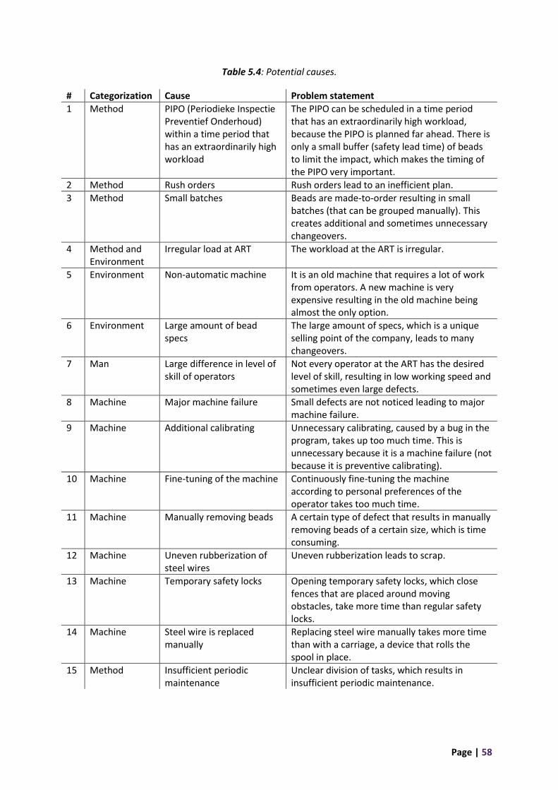
Page | 58
Table 5.4: Potential causes.
# Categorization Cause Problem statement
1 Method PIPO (Periodieke Inspectie Preventief Onderhoud) within a time period that has an extraordinarily high workload
The PIPO can be scheduled in a time period that has an extraordinarily high workload, because the PIPO is planned far ahead. There is only a small buffer (safety lead time) of beads to limit the impact, which makes the timing of the PIPO very important.
2 Method Rush orders Rush orders lead to an inefficient plan.
3 Method Small batches Beads are made-to-order resulting in small batches (that can be grouped manually). This creates additional and sometimes unnecessary changeovers.
4 Method and Environment
Irregular load at ART The workload at the ART is irregular.
5 Environment Non-automatic machine It is an old machine that requires a lot of work from operators. A new machine is very expensive resulting in the old machine being almost the only option.
6 Environment Large amount of bead specs
The large amount of specs, which is a unique selling point of the company, leads to many changeovers.
7 Man Large difference in level of skill of operators
Not every operator at the ART has the desired level of skill, resulting in low working speed and sometimes even large defects.
8 Machine Major machine failure Small defects are not noticed leading to major machine failure.
9 Machine Additional calibrating Unnecessary calibrating, caused by a bug in the program, takes up too much time. This is unnecessary because it is a machine failure (not because it is preventive calibrating).
10 Machine Fine-tuning of the machine Continuously fine-tuning the machine according to personal preferences of the operator takes too much time.
11 Machine Manually removing beads A certain type of defect that results in manually removing beads of a certain size, which is time consuming.
12 Machine Uneven rubberization of steel wires
Uneven rubberization leads to scrap.
13 Machine Temporary safety locks Opening temporary safety locks, which close fences that are placed around moving obstacles, take more time than regular safety locks.
14 Machine Steel wire is replaced manually
Replacing steel wire manually takes more time than with a carriage, a device that rolls the spool in place.
15 Method Insufficient periodic maintenance
Unclear division of tasks, which results in insufficient periodic maintenance.
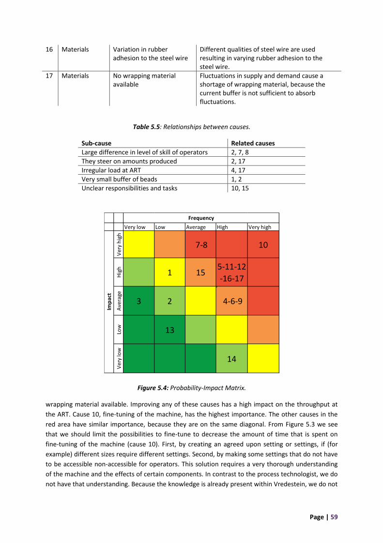
Page | 59
16 Materials Variation in rubber adhesion to the steel wire
Different qualities of steel wire are used resulting in varying rubber adhesion to the steel wire.
17 Materials No wrapping material available
Fluctuations in supply and demand cause a shortage of wrapping material, because the current buffer is not sufficient to absorb fluctuations.
Table 5.5: Relationships between causes.
Sub-cause Related causes
Large difference in level of skill of operators 2, 7, 8
They steer on amounts produced 2, 17
Irregular load at ART 4, 17
Very small buffer of beads 1, 2
Unclear responsibilities and tasks 10, 15
Figure 5.4: Probability-Impact Matrix.
wrapping material available. Improving any of these causes has a high impact on the throughput at
the ART. Cause 10, fine-tuning of the machine, has the highest importance. The other causes in the
red area have similar importance, because they are on the same diagonal. From Figure 5.3 we see
that we should limit the possibilities to fine-tune to decrease the amount of time that is spent on
fine-tuning of the machine (cause 10). First, by creating an agreed upon setting or settings, if (for
example) different sizes require different settings. Second, by making some settings that do not have
to be accessible non-accessible for operators. This solution requires a very thorough understanding
of the machine and the effects of certain components. In contrast to the process technologist, we do
not have that understanding. Because the knowledge is already present within Vredestein, we do not
Very low Low Average High Very high
Ver
y h
igh
7-8 10
Hig
h
1 155-11-12
-16-17
Ave
rage
3 2 4-6-9
Low 13
Ver
y lo
w
14
Frequency
Imp
act
Page | 60
continue to improve this cause and give the process technologist the recommendation to continue.
We further elaborate on the implementation of the recommendation in Chapter 6. The other causes
within the red area have a similar level of importance. We decide to focus on cause 17: no wrapping
material, because the sub-causes are more related to our field of expertise and there we could
contribute most. The other causes in the red area have technical issues that are material or machine
specific. Here the same reasoning applies, it is not related to our field of expertise and the knowledge
is present within Vredestein. We communicate these causes with the business team manager who
can allocate the issues to the employees with the right skills. Thus, finding solutions for (some of) the
other causes is a recommendation for further research if the ART remains the bottleneck. To validate
our choice, we assess the impact of wrapping material on starvation at the ART. We cannot validate
all causes in the probability-impact matrix, because some are not booked or the bookings do not
specify whether it is a problem. For instance, the amount of fine-tuning is booked, but we do not
know which part is required and which part is not necessary. Thus, this number does not indicate if
the fine-tuning can be reduced. For starvation on wrapping material we know every minute is a loss
that is not necessary. From the data, period 14/1/2019-31/3/2019, we gather the total amount of
booked starvation caused by wrapping material. This adds up to 1,050 minutes of starvation caused
by wrapping material. The total available time is 110,400, which means that we gain 0.95% of time if
we can eliminate starvation caused by wrapping material.
We see from Figure 5.3 that we can tackle five sub-causes to improve the throughput at the ART
caused by no wrapping material. These five sub-causes are the following:
• Length of a roll wrapping material is not measured and not booked
• Large defects at the ORION
• Vredestein steers on amounts produced
• Irregular load at the ART
• The current buffer for wrapping material is not sufficient
We do not look into the irregular load at the ART, because this only causes a shortage of wrapping
material if the ART is ahead of schedule, see Appendix 3. Also, we do not look into large defects at
the ORION, because it is a technical issue of the machine and not our field of expertise. If this is still
an opportunity for improvement after improving other sub-causes it can be allocated to the
employees with the right skills. Their current KPIs motivate to produce high amounts of tyres, but not
necessarily to deliver the demand of the next station. The impact it has on the throughput of the
system is unclear, but it is identified as an issue throughout the entire factory. The project team has
decided to revise the current KPIs according to the concept of TOC. They started for PCT and plan to
continue for AGRI and SM. Thus, we do not look into revising the current KPIs. This leaves us with
two sub-causes to improve. The first sub-cause is “the length of a roll of wrapping material is not
measured and not booked”. The second sub-cause is “the current buffer for wrapping material is not
sufficient”. Improving these sub-causes results in ensuring the right materials at the right time.
5.3 Subordinate non-bottleneck processes In this section we execute the two phases of the process to subordinate all non-bottleneck processes.
We start with Phase 6 in Section 5.3.1. In this section we discuss data on the length of a roll of
wrapping material. Section 5.3.2 continues with Phase 6 by setting up the inventory control policy.
Section 5.3.3 executes Phase 7 and gives options for implementation and recommendation.
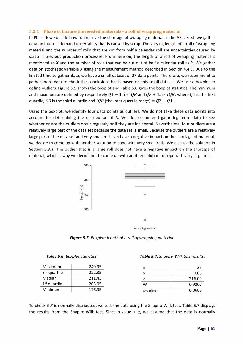
Page | 61
5.3.1 Phase 6: Ensure the needed materials - a roll of wrapping material
In Phase 6 we decide how to improve the shortage of wrapping material at the ART. First, we gather
data on internal demand uncertainty that is caused by scrap. The varying length of a roll of wrapping
material and the number of rolls that are cut from half a calendar roll are uncertainties caused by
scrap in previous production processes. From here on, the length of a roll of wrapping material is
mentioned as X and the number of rolls that can be cut out of half a calendar roll as Y. We gather
data on stochastic variable X using the measurement method described in Section 4.4.1. Due to the
limited time to gather data, we have a small dataset of 27 data points. Therefore, we recommend to
gather more data to check the conclusion that is based on this small dataset. We use a boxplot to
define outliers. Figure 5.5 shows the boxplot and Table 5.6 gives the boxplot statistics. The minimum
and maximum are defined by respectively 𝑄1 − 1.5 ∗ 𝐼𝑄𝑅 and 𝑄3 + 1.5 ∗ 𝐼𝑄𝑅, where 𝑄1 is the first
quartile, 𝑄3 is the third quartile and 𝐼𝑄𝑅 (the inter quartile range) = 𝑄3 − 𝑄1.
Using the boxplot, we identify four data points as outliers. We do not take these data points into
account for determining the distribution of X. We do recommend gathering more data to see
whether or not the outliers occur regularly or if they are incidental. Nevertheless, four outliers are a
relatively large part of the data set because the data set is small. Because the outliers are a relatively
large part of the data set and very small rolls can have a negative impact on the shortage of material,
we decide to come up with another solution to cope with very small rolls. We discuss the solution in
Section 5.3.3. The outlier that is a large roll does not have a negative impact on the shortage of
material, which is why we decide not to come up with another solution to cope with very large rolls.
Table 5.6: Boxplot statistics.
Maximum 249.95
3rd quartile 222.35
Median 211.43
1st quartile 203.95
Minimum 176.35
Table 5.7: Shapiro-Wilk test results.
n 23
α 0.05
�̅� 216.09
W 0.9207
p-value 0.0689
To check if X is normally distributed, we test the data using the Shapiro-Wilk test. Table 5.7 displays
the results from the Shapiro-Wilk test. Since p-value > α, we assume that the data is normally
Figure 5.5: Boxplot: length of a roll of wrapping material.
Page | 62
distributed. In other words, the difference between the data sample and the normal distribution is
not big enough to be statistically significant.
The 2nd and 3rd column of Table 5.8 display the characteristics of X (𝜇𝑋 and 𝜎𝑋). We see that the
average length on a roll is lower than the assumption of 250 meter. To decide whether we should
update the assumption of 250 meters per roll, we conduct a left tailed hypothesis test. In the test we
set 𝐻0: 𝜇 ≥ 250 and 𝐻1: 𝜇 < 250, where the level of significance, α, equals 1%. We know the
standard deviation of the sampling test, but we do not know the standard deviation of the
population. Thus, we use a t-distribution with 𝑛 − 1 degrees of freedom (𝑑𝑓). Table 5.9 shows the
results of the left tailed hypothesis test. From the table follows that the critical region is
(−∞, 243.7]. �̅� = 216.1 meters and is within the critical region, therefore we reject 𝐻0. This means
that we do want to update the assumption of 250 meters per roll. We set the expected length of a
roll of wrapping material to the rounded average of the sampling test, which equals 216 meters.
Table 5.8: Characteristics of wrapping material.
Name 𝝁𝑿 𝝈𝑿 𝝁𝒀 𝝈𝒀 𝑬(𝑿𝒀) 𝑽𝑨𝑹(𝑿𝒀)
HE01-00-0034 216.09 12.05 9.53 0.50 2060.55 24859.73
HE01-00-0038 216.09 12.05 8.26 0.44 1783.85 18803.20
Table 5.9: Hypothesis test results.
n 23
df 22
α 0.01
𝑧 -2.508
𝑥𝑘 243.7
�̅� 216.1
The number of rolls that can be cut out of half a calendar roll, Y, has a discrete distribution. From
data on historic orders of wrapping material (that is already available) we gather the following: for
HE01-00-0034, 9 rolls can be cut from half a calendar roll with a chance of 0.46 and 10 rolls with a
chance of 0.54. For HE01-00-0038 8 rolls can be cut from half a calendar roll with a chance of 0.74
and 9 rolls with a chance of 0.26. Next, we calculate μY and σY , the mean and standard deviation of
the number of rolls per batch, using Equation 5-1. We add the characteristics of Y (𝜇𝑌 and 𝜎𝑌). in
Table 5.8. The variation in the number of rolls does not affect the accuracy of the inventory in the
system, because each roll is booked.
Equation 5-1: Mean and standard deviation in case of a discrete distribution.
𝝁 = ∑ 𝑝𝑖𝑥𝑖𝑛𝑖
𝝈 = √∑ 𝑝𝑖(𝑥𝑖 − 𝜇)2𝑛𝑖
𝑝𝑖: 𝑥𝑖:
𝑃𝑟𝑜𝑏𝑎𝑏𝑖𝑙𝑖𝑡𝑦 𝑜𝑓 𝑥𝑖 𝑉𝑎𝑙𝑢𝑒 𝑜𝑓 𝑖
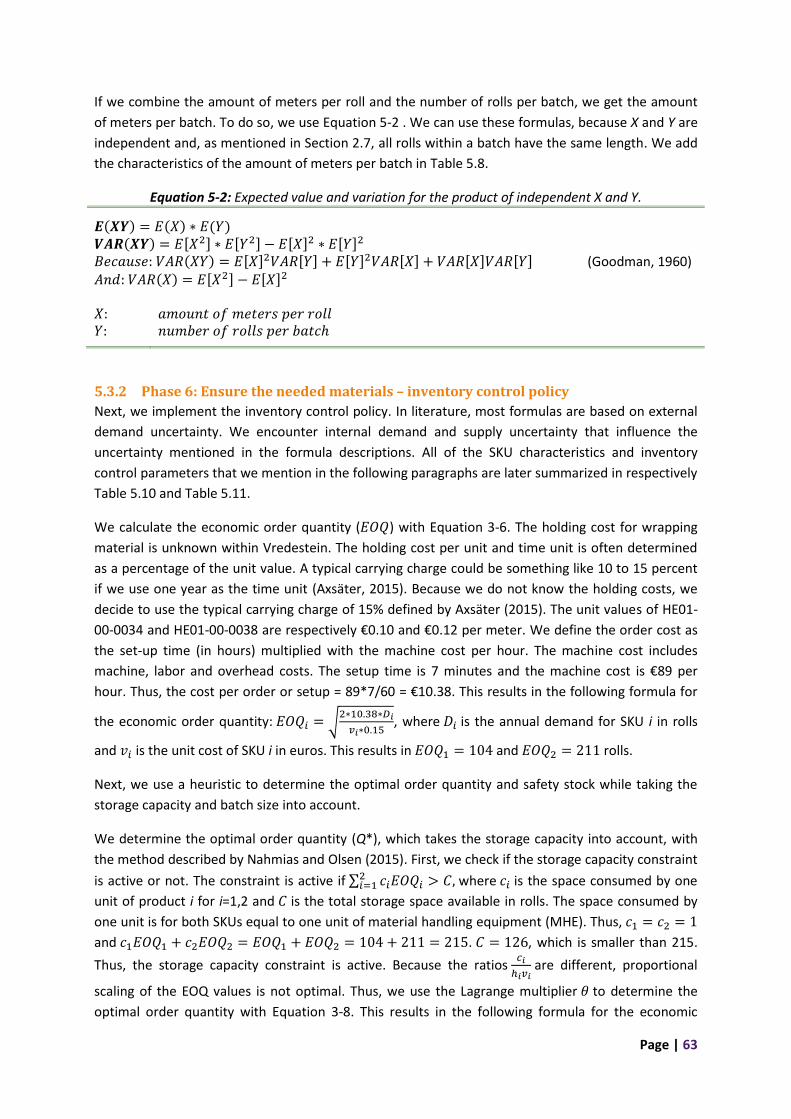
Page | 63
If we combine the amount of meters per roll and the number of rolls per batch, we get the amount
of meters per batch. To do so, we use Equation 5-2 . We can use these formulas, because X and Y are
independent and, as mentioned in Section 2.7, all rolls within a batch have the same length. We add
the characteristics of the amount of meters per batch in Table 5.8.
Equation 5-2: Expected value and variation for the product of independent X and Y.
𝑬(𝑿𝒀) = 𝐸(𝑋) ∗ 𝐸(𝑌) 𝑽𝑨𝑹(𝑿𝒀) = 𝐸[𝑋2] ∗ 𝐸[𝑌2] − 𝐸[𝑋]2 ∗ 𝐸[𝑌]2 𝐵𝑒𝑐𝑎𝑢𝑠𝑒: 𝑉𝐴𝑅(𝑋𝑌) = 𝐸[𝑋]2𝑉𝐴𝑅[𝑌] + 𝐸[𝑌]2𝑉𝐴𝑅[𝑋] + 𝑉𝐴𝑅[𝑋]𝑉𝐴𝑅[𝑌] (Goodman, 1960) 𝐴𝑛𝑑: 𝑉𝐴𝑅(𝑋) = 𝐸[𝑋2] − 𝐸[𝑋]2
𝑋: 𝑌:
𝑎𝑚𝑜𝑢𝑛𝑡 𝑜𝑓 𝑚𝑒𝑡𝑒𝑟𝑠 𝑝𝑒𝑟 𝑟𝑜𝑙𝑙 𝑛𝑢𝑚𝑏𝑒𝑟 𝑜𝑓 𝑟𝑜𝑙𝑙𝑠 𝑝𝑒𝑟 𝑏𝑎𝑡𝑐ℎ
5.3.2 Phase 6: Ensure the needed materials – inventory control policy
Next, we implement the inventory control policy. In literature, most formulas are based on external
demand uncertainty. We encounter internal demand and supply uncertainty that influence the
uncertainty mentioned in the formula descriptions. All of the SKU characteristics and inventory
control parameters that we mention in the following paragraphs are later summarized in respectively
Table 5.10 and Table 5.11.
We calculate the economic order quantity (𝐸𝑂𝑄) with Equation 3-6. The holding cost for wrapping
material is unknown within Vredestein. The holding cost per unit and time unit is often determined
as a percentage of the unit value. A typical carrying charge could be something like 10 to 15 percent
if we use one year as the time unit (Axsäter, 2015). Because we do not know the holding costs, we
decide to use the typical carrying charge of 15% defined by Axsäter (2015). The unit values of HE01-
00-0034 and HE01-00-0038 are respectively €0.10 and €0.12 per meter. We define the order cost as
the set-up time (in hours) multiplied with the machine cost per hour. The machine cost includes
machine, labor and overhead costs. The setup time is 7 minutes and the machine cost is €89 per
hour. Thus, the cost per order or setup = 89*7/60 = €10.38. This results in the following formula for
the economic order quantity: 𝐸𝑂𝑄𝑖 = √2∗10.38∗𝐷𝑖
𝑣𝑖∗0.15, where 𝐷𝑖 is the annual demand for SKU i in rolls
and 𝑣𝑖 is the unit cost of SKU i in euros. This results in 𝐸𝑂𝑄1 = 104 and 𝐸𝑂𝑄2 = 211 rolls.
Next, we use a heuristic to determine the optimal order quantity and safety stock while taking the
storage capacity and batch size into account.
We determine the optimal order quantity (Q*), which takes the storage capacity into account, with
the method described by Nahmias and Olsen (2015). First, we check if the storage capacity constraint
is active or not. The constraint is active if ∑ 𝑐𝑖𝐸𝑂𝑄𝑖2𝑖=1 > 𝐶, where 𝑐𝑖 is the space consumed by one
unit of product i for i=1,2 and 𝐶 is the total storage space available in rolls. The space consumed by
one unit is for both SKUs equal to one unit of material handling equipment (MHE). Thus, 𝑐1 = 𝑐2 = 1
and 𝑐1𝐸𝑂𝑄1 + 𝑐2𝐸𝑂𝑄2 = 𝐸𝑂𝑄1 + 𝐸𝑂𝑄2 = 104 + 211 = 215. 𝐶 = 126, which is smaller than 215.
Thus, the storage capacity constraint is active. Because the ratios 𝑐𝑖
ℎ𝑖𝑣𝑖 are different, proportional
scaling of the EOQ values is not optimal. Thus, we use the Lagrange multiplier 𝜃 to determine the
optimal order quantity with Equation 3-8. This results in the following formula for the economic
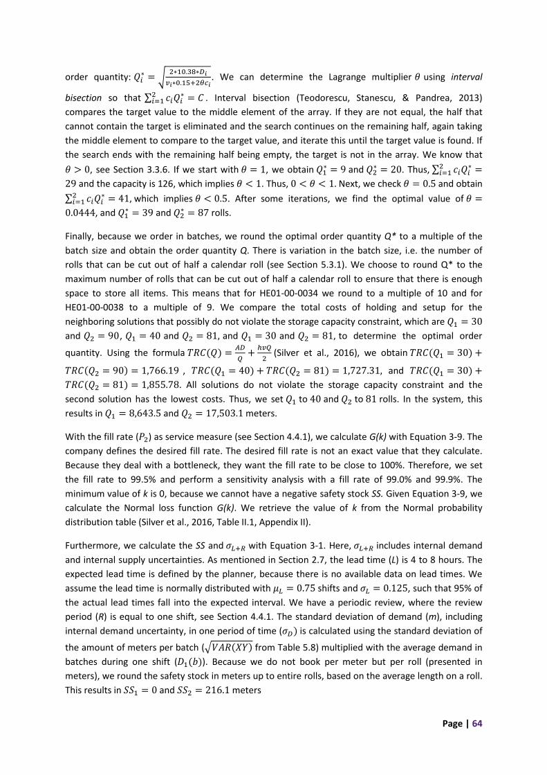
Page | 64
order quantity: 𝑄𝑖∗ = √
2∗10.38∗𝐷𝑖
𝑣𝑖∗0.15+2𝜃𝑐𝑖. We can determine the Lagrange multiplier 𝜃 using interval
bisection so that ∑ 𝑐𝑖𝑄𝑖∗2
𝑖=1 = 𝐶 . Interval bisection (Teodorescu, Stanescu, & Pandrea, 2013)
compares the target value to the middle element of the array. If they are not equal, the half that
cannot contain the target is eliminated and the search continues on the remaining half, again taking
the middle element to compare to the target value, and iterate this until the target value is found. If
the search ends with the remaining half being empty, the target is not in the array. We know that
𝜃 > 0, see Section 3.3.6. If we start with 𝜃 = 1, we obtain 𝑄1∗ = 9 and 𝑄2
∗ = 20. Thus, ∑ 𝑐𝑖𝑄𝑖∗2
𝑖=1 =
29 and the capacity is 126, which implies 𝜃 < 1. Thus, 0 < 𝜃 < 1. Next, we check 𝜃 = 0.5 and obtain
∑ 𝑐𝑖𝑄𝑖∗2
𝑖=1 = 41, which implies 𝜃 < 0.5. After some iterations, we find the optimal value of 𝜃 =
0.0444, and 𝑄1∗ = 39 and 𝑄2
∗ = 87 rolls.
Finally, because we order in batches, we round the optimal order quantity Q* to a multiple of the
batch size and obtain the order quantity Q. There is variation in the batch size, i.e. the number of
rolls that can be cut out of half a calendar roll (see Section 5.3.1). We choose to round Q* to the
maximum number of rolls that can be cut out of half a calendar roll to ensure that there is enough
space to store all items. This means that for HE01-00-0034 we round to a multiple of 10 and for
HE01-00-0038 to a multiple of 9. We compare the total costs of holding and setup for the
neighboring solutions that possibly do not violate the storage capacity constraint, which are 𝑄1 = 30
and 𝑄2 = 90, 𝑄1 = 40 and 𝑄2 = 81, and 𝑄1 = 30 and 𝑄2 = 81, to determine the optimal order
quantity. Using the formula 𝑇𝑅𝐶(𝑄) =𝐴𝐷
𝑄+
ℎ𝑣𝑄
2 (Silver et al., 2016), we obtain 𝑇𝑅𝐶(𝑄1 = 30) +
𝑇𝑅𝐶(𝑄2 = 90) = 1,766.19 , 𝑇𝑅𝐶(𝑄1 = 40) + 𝑇𝑅𝐶(𝑄2 = 81) = 1,727.31, and 𝑇𝑅𝐶(𝑄1 = 30) +
𝑇𝑅𝐶(𝑄2 = 81) = 1,855.78. All solutions do not violate the storage capacity constraint and the
second solution has the lowest costs. Thus, we set 𝑄1 to 40 and 𝑄2 to 81 rolls. In the system, this
results in 𝑄1 = 8,643.5 and 𝑄2 = 17,503.1 meters.
With the fill rate (𝑃2) as service measure (see Section 4.4.1), we calculate G(k) with Equation 3-9. The
company defines the desired fill rate. The desired fill rate is not an exact value that they calculate.
Because they deal with a bottleneck, they want the fill rate to be close to 100%. Therefore, we set
the fill rate to 99.5% and perform a sensitivity analysis with a fill rate of 99.0% and 99.9%. The
minimum value of k is 0, because we cannot have a negative safety stock SS. Given Equation 3-9, we
calculate the Normal loss function G(k). We retrieve the value of k from the Normal probability
distribution table (Silver et al., 2016, Table II.1, Appendix II).
Furthermore, we calculate the SS and 𝜎𝐿+𝑅 with Equation 3-1. Here, 𝜎𝐿+𝑅 includes internal demand
and internal supply uncertainties. As mentioned in Section 2.7, the lead time (L) is 4 to 8 hours. The
expected lead time is defined by the planner, because there is no available data on lead times. We
assume the lead time is normally distributed with 𝜇𝐿 = 0.75 shifts and 𝜎𝐿 = 0.125, such that 95% of
the actual lead times fall into the expected interval. We have a periodic review, where the review
period (R) is equal to one shift, see Section 4.4.1. The standard deviation of demand (m), including
internal demand uncertainty, in one period of time (𝜎𝐷) is calculated using the standard deviation of
the amount of meters per batch (√𝑉𝐴𝑅(𝑋𝑌) from Table 5.8) multiplied with the average demand in
batches during one shift (𝐷1(𝑏)). Because we do not book per meter but per roll (presented in
meters), we round the safety stock in meters up to entire rolls, based on the average length on a roll.
This results in 𝑆𝑆1 = 0 and 𝑆𝑆2 = 216.1 meters
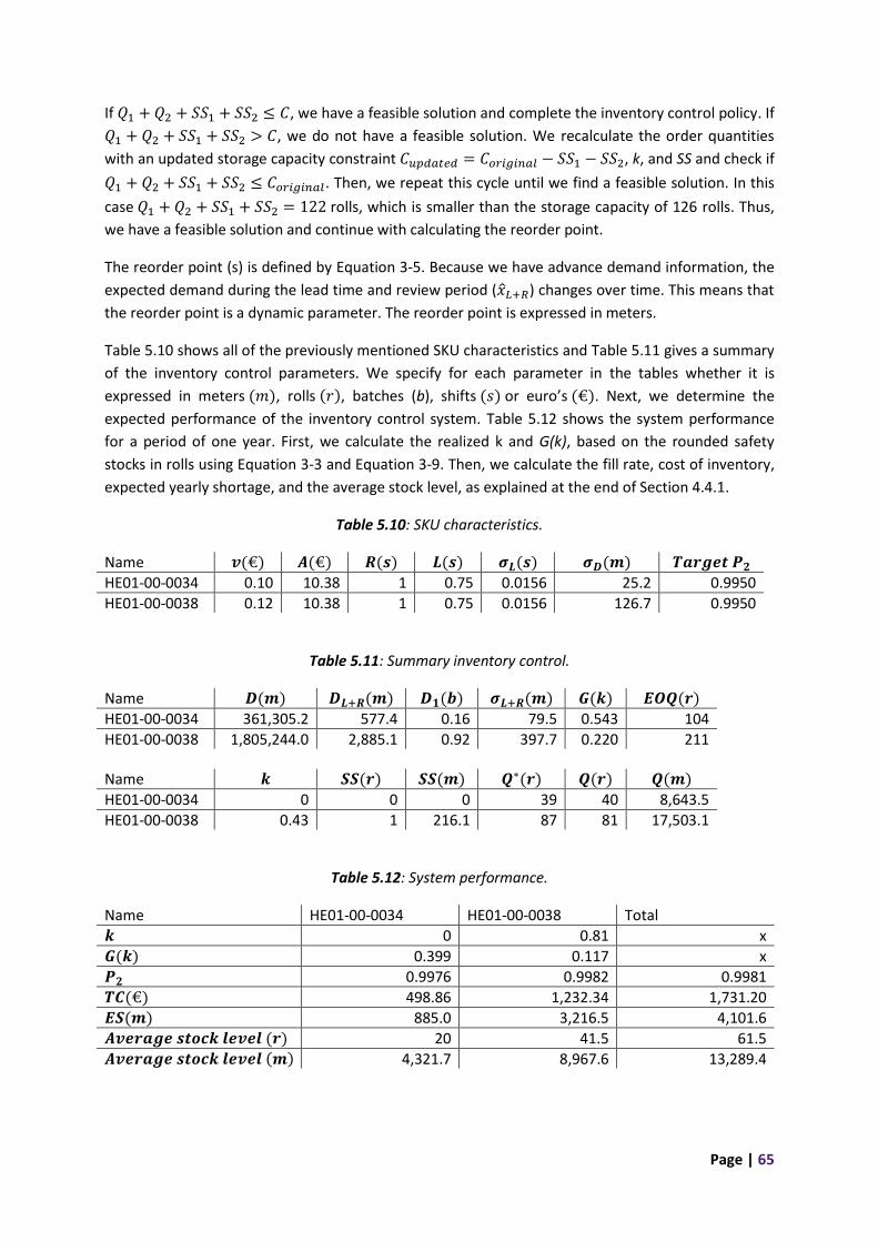
Page | 65
If 𝑄1 + 𝑄2 + 𝑆𝑆1 + 𝑆𝑆2 ≤ 𝐶, we have a feasible solution and complete the inventory control policy. If
𝑄1 + 𝑄2 + 𝑆𝑆1 + 𝑆𝑆2 > 𝐶, we do not have a feasible solution. We recalculate the order quantities
with an updated storage capacity constraint 𝐶𝑢𝑝𝑑𝑎𝑡𝑒𝑑 = 𝐶𝑜𝑟𝑖𝑔𝑖𝑛𝑎𝑙 − 𝑆𝑆1 − 𝑆𝑆2, k, and SS and check if
𝑄1 + 𝑄2 + 𝑆𝑆1 + 𝑆𝑆2 ≤ 𝐶𝑜𝑟𝑖𝑔𝑖𝑛𝑎𝑙. Then, we repeat this cycle until we find a feasible solution. In this
case 𝑄1 + 𝑄2 + 𝑆𝑆1 + 𝑆𝑆2 = 122 rolls, which is smaller than the storage capacity of 126 rolls. Thus,
we have a feasible solution and continue with calculating the reorder point.
The reorder point (s) is defined by Equation 3-5. Because we have advance demand information, the
expected demand during the lead time and review period (𝑥𝐿+𝑅) changes over time. This means that
the reorder point is a dynamic parameter. The reorder point is expressed in meters.
Table 5.10 shows all of the previously mentioned SKU characteristics and Table 5.11 gives a summary
of the inventory control parameters. We specify for each parameter in the tables whether it is
expressed in meters (𝑚), rolls (𝑟), batches (b), shifts (𝑠) or euro’s (€). Next, we determine the
expected performance of the inventory control system. Table 5.12 shows the system performance
for a period of one year. First, we calculate the realized k and G(k), based on the rounded safety
stocks in rolls using Equation 3-3 and Equation 3-9. Then, we calculate the fill rate, cost of inventory,
expected yearly shortage, and the average stock level, as explained at the end of Section 4.4.1.
Table 5.10: SKU characteristics.
Name 𝒗(€) 𝑨(€) 𝑹(𝒔) 𝑳(𝒔) 𝝈𝑳(𝒔) 𝝈𝑫(𝒎) 𝑻𝒂𝒓𝒈𝒆𝒕 𝑷𝟐
HE01-00-0034 0.10 10.38 1 0.75 0.0156 25.2 0.9950
HE01-00-0038 0.12 10.38 1 0.75 0.0156 126.7 0.9950
Table 5.11: Summary inventory control.
Name 𝑫(𝒎) 𝑫𝑳+𝑹(𝒎) 𝑫𝟏(𝒃) 𝝈𝑳+𝑹(𝒎) 𝑮(𝒌) 𝑬𝑶𝑸(𝒓)
HE01-00-0034 361,305.2 577.4 0.16 79.5 0.543 104
HE01-00-0038 1,805,244.0 2,885.1 0.92 397.7 0.220 211 Name 𝒌 𝑺𝑺(𝒓) 𝑺𝑺(𝒎) 𝑸∗(𝒓) 𝑸(𝒓) 𝑸(𝒎)
HE01-00-0034 0 0 0 39 40 8,643.5
HE01-00-0038 0.43 1 216.1 87 81 17,503.1
Table 5.12: System performance.
Name HE01-00-0034 HE01-00-0038 Total
𝒌 0 0.81 x
𝑮(𝒌) 0.399 0.117 x
𝑷𝟐 0.9976 0.9982 0.9981
𝑻𝑪(€) 498.86 1,232.34 1,731.20
𝑬𝑺(𝒎) 885.0 3,216.5 4,101.6
𝑨𝒗𝒆𝒓𝒂𝒈𝒆 𝒔𝒕𝒐𝒄𝒌 𝒍𝒆𝒗𝒆𝒍 (𝒓) 20 41.5 61.5
𝑨𝒗𝒆𝒓𝒂𝒈𝒆 𝒔𝒕𝒐𝒄𝒌 𝒍𝒆𝒗𝒆𝒍 (𝒎) 4,321.7 8,967.6 13,289.4
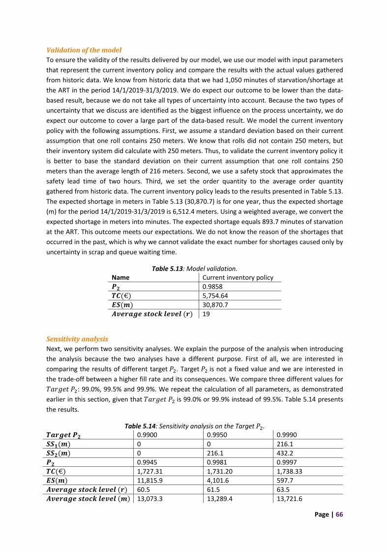
Page | 66
Validation of the model
To ensure the validity of the results delivered by our model, we use our model with input parameters
that represent the current inventory policy and compare the results with the actual values gathered
from historic data. We know from historic data that we had 1,050 minutes of starvation/shortage at
the ART in the period 14/1/2019-31/3/2019. We do expect our outcome to be lower than the data-
based result, because we do not take all types of uncertainty into account. Because the two types of
uncertainty that we discuss are identified as the biggest influence on the process uncertainty, we do
expect our outcome to cover a large part of the data-based result. We model the current inventory
policy with the following assumptions. First, we assume a standard deviation based on their current
assumption that one roll contains 250 meters. We know that rolls did not contain 250 meters, but
their inventory system did calculate with 250 meters. Thus, to validate the current inventory policy it
is better to base the standard deviation on their current assumption that one roll contains 250
meters than the average length of 216 meters. Second, we use a safety stock that approximates the
safety lead time of two hours. Third, we set the order quantity to the average order quantity
gathered from historic data. The current inventory policy leads to the results presented in Table 5.13.
The expected shortage in meters in Table 5.13 (30,870.7) is for one year, thus the expected shortage
(m) for the period 14/1/2019-31/3/2019 is 6,512.4 meters. Using a weighted average, we convert the
expected shortage in meters into minutes. The expected shortage equals 893.7 minutes of starvation
at the ART. This outcome meets our expectations. We do not know the reason of the shortages that
occurred in the past, which is why we cannot validate the exact number for shortages caused only by
uncertainty in scrap and queue waiting time.
Table 5.13: Model validation. Name Current inventory policy
𝑷𝟐 0.9858
𝑻𝑪(€) 5,754.64
𝑬𝑺(𝒎) 30,870.7
𝑨𝒗𝒆𝒓𝒂𝒈𝒆 𝒔𝒕𝒐𝒄𝒌 𝒍𝒆𝒗𝒆𝒍 (𝒓) 19
Sensitivity analysis
Next, we perform two sensitivity analyses. We explain the purpose of the analysis when introducing
the analysis because the two analyses have a different purpose. First of all, we are interested in
comparing the results of different target 𝑃2. Target 𝑃2 is not a fixed value and we are interested in
the trade-off between a higher fill rate and its consequences. We compare three different values for
𝑇𝑎𝑟𝑔𝑒𝑡 𝑃2: 99.0%, 99.5% and 99.9%. We repeat the calculation of all parameters, as demonstrated
earlier in this section, given that 𝑇𝑎𝑟𝑔𝑒𝑡 𝑃2 is 99.0% or 99.9% instead of 99.5%. Table 5.14 presents
the results.
Table 5.14: Sensitivity analysis on the Target 𝑃2. 𝑻𝒂𝒓𝒈𝒆𝒕 𝑷𝟐 0.9900 0.9950 0.9990
𝑺𝑺𝟏(𝒎) 0 0 216.1
𝑺𝑺𝟐(𝒎) 0 216.1 432.2
𝑷𝟐 0.9945 0.9981 0.9997
𝑻𝑪(€) 1,727.31 1,731.20 1,738.33
𝑬𝑺(𝒎) 11,815.9 4,101.6 597.7
𝑨𝒗𝒆𝒓𝒂𝒈𝒆 𝒔𝒕𝒐𝒄𝒌 𝒍𝒆𝒗𝒆𝒍 (𝒓) 60.5 61.5 63.5
𝑨𝒗𝒆𝒓𝒂𝒈𝒆 𝒔𝒕𝒐𝒄𝒌 𝒍𝒆𝒗𝒆𝒍 (𝒎) 13,073.3 13,289.4 13,721.6

Page | 67
We see that the change in fill rate has a small effect on both costs and stock level. This is caused by
the margin of capacity left unutilized with the order quantity rounded to batches. The safety stock
uses this excess of capacity and therefore the order quantity stays the same. Furthermore, the
amount of safety stock needed to achieve those service levels are relatively small.
Next, we perform a sensitivity analysis for the carrying charge. The carrying charge of 15% is based
on a rule of thumb and does not necessarily represent the real cost of inventory. To see the influence
of this assumption on the relevance of our inventory control policy, we perform a sensitivity analysis.
Table 5.15 presents the results of the sensitivity analysis. Changing the carrying charge to 10-40%
only changes the costs, because the storage capacity also limits the order quantity for these values
(not the EOQ). This means that the defined policy is still relevant if the carrying charge deviates
slightly and only the costs change.
Table 5.15: Sensitivity analysis on the carrying charge 𝒉 0.10 0.15 0.20 0.40
𝑷𝟐 0.9981 0.9981 0.9981 0.9981
𝑻𝑪(€) 1,655.78 1,731.20 1,806.61 2,108.27
𝑬𝑺(𝒎) 4,101.6 4,101.6 4,101.6 4,101.6
𝑨𝒗𝒆𝒓𝒂𝒈𝒆 𝒔𝒕𝒐𝒄𝒌 𝒍𝒆𝒗𝒆𝒍 (𝒓) 61.5 61.5 61.5 61.5
𝑨𝒗𝒆𝒓𝒂𝒈𝒆 𝒔𝒕𝒐𝒄𝒌 𝒍𝒆𝒗𝒆𝒍 (𝒎) 13,289.4 13,289.4 13,289.4 13,289.4
5.3.3 Phase 7: Implementation and recommendations
In Phase 7 we discuss the recommendations for implementation. All recommendations that require
an alteration in PIBS are discussed with an employee who can implement alterations. He confirmed
that all options discussed below are possible concerning PIBS.
First, we recommend to change the assumption of 250 meters per roll of wrapping material to 216
meters to increase the accuracy of the inventory. This requires a change in PIBS. The amount of
meters that are automatically booked per roll can easily be changed in PIBS.
We recommend to expand this option with a solution for the small rolls that are identified as an
outlier in Section 5.3.1. For these small rolls, we do want to adjust the amount of meters per roll in
the system. We can measure the diameter manually, as described in Section 4.4.1, and estimate the
length of the roll using Equation 4-1. The operator can use the template that will be hanging in the
working area of the ORION to identify the outliers. The template shows the minimum size of a roll,
176 meters, without becoming an outlier. The operator can hold the roll in front of the template. If
the roll is smaller than the roll on the template, the diameter should be measured and entered in the
system manually. This solution requires a new template, and alternation in PIBS to enable entering
the amount of meters manually. A proposition for the template is given in Appendix 5.
If the shortage of wrapping material has improved sufficiently (by assessment of Apollo Vredestein),
we recommend to maintain this solution. If it has not improved sufficiently, we recommend to
measure the length of a roll in each batch. This will increase the accuracy of the inventory in the
system, but it comes at a cost. There are two options to add a measurement to the roll. First, we can
measure the diameter manually and enter the diameter in PIBS and with that estimate the
corresponding length. This option does not need an initial investment, but requires time from the
operators. Implementing this option also requires alternation in PIBS. We need to add an option to
Page | 68
enter the amount of meters manually. Second, we can install measuring equipment at the ORION.
The measuring equipment measures the length of the wrapping material while it rolls up the material
on the material handling equipment. This option requires an initial investment but does not include
additional tasks for the operators. The second option also requires alternation in PIBS, because the
data gathered by the measurement equipment needs to be processed in PIBS.
Regarding the inventory control policy we recommend to implement a (R,s,Q) policy as described in
Section 5.3.2. With a small amount of safety stock we see a large improvement in the amount of
shortage compared to the current policy mentioned in the validation of the model. We recommend
to set the target of 𝑃2 to 0.999. From the sensitivity analysis we see that increasing the fill rate
requires a small amount of extra stock and a small increase in costs. The needed storage space is
already available, which means that the required investment is low. Implementing the policy in PIBS
requires small changes. Only the order quantity needs to be adjusted to 𝑄1 = 8,643.5 and 𝑄2 =
17,503.1, and the current reorder point needs to increase with a safety stock of 𝑆𝑆1 = 216.1 or
𝑆𝑆2 = 432.2 meters.
5.4 Conclusion In this chapter we implemented the model. In Section 5.1 we executed the bottleneck identification
process. In Phase 1 we excluded machines with a GAP > 50%. In Phase 2 the turning point method
identified the ART as the most significant bottleneck. In Phase 3 the utilization method also identified
the ART as the most significant bottleneck. Finally, Phase 4 stated that Phases 2 and 3 coincide and
concluded on the ART as the most significant bottleneck. We validated the outcome with the
knowledge of the daily state of affairs.
In Section 5.2 we executed the bottleneck optimization process. We formulated the problem as
“limited throughput at the ART”. We presented an overview of the potential causes using an
Ishikawa diagram and we arranged the potential causes in a Probability-Impact Matrix. Using this
matrix, we decided to focus on the cause “no wrapping material” and specifically on the two sub-
causes “the length of a roll is not measured and not booked” and “the current buffer for wrapping
material is not sufficient”.
In Section 5.3 we executed the process to subordinate all non-bottleneck processes. First, we
gathered and analyzed the data on the length of a roll of wrapping material. We concluded that the
assumption by Apollo Vredestein of 250 meters on a roll should be updated to 216 meters. Second,
we set up an (R,s,Q) inventory control policy and presented the parameters. We also presented the
performance of the system, we validated the model and performed a sensitivity analysis. Finally, we
provided recommendations regarding wrapping material and the inventory control policy.

Page | 69
6. Conclusion, recommendations and discussion In this chapter we conclude on the main research questions in Section 6.1. In Section 6.2 we give an
overview of the recommendations made throughout this research. Finally, Section 6.3 discusses the
limitations of this research.
6.1 Conclusion To achieve both lower costs per tyre and a higher throughput, we decided to improve performance
by following the concept called Theory of Constraints. In this section we answer the main research
question:
“How can Apollo Vredestein identify the most significant bottleneck machine within the production
line of agricultural and space master tyres, improve the most significant bottleneck machine, and
align non-bottleneck machines to increase the throughput of the system?”
To identify the most significant bottleneck we developed a bottleneck identification process. The
bottleneck identification process consists of four phases. The first phase filters on data availability to
identify non-bottlenecks. The second phase performs the turning point method and the third phase
performs the utilization method to identify the most significant bottleneck. Finally, the fourth phase
gives a conclusion on the location of the bottleneck and validates the result. Apollo Vredestein can
identify the most significant bottleneck by using the supportive dashboard (see Appendix 2) while
executing these phases.
In the current situation we concluded that the most significant bottleneck is a machine called the
ART. The ART is a bead-making machine that produces both AGRI and SM beads. We have found
multiple causes that Apollo Vredestein can improve to achieve a high impact on the throughput at
the ART. Nevertheless, fine-tuning of the machine has the highest importance. To decrease the
amount of time that is spent on fine-tuning of the machine, Apollo Vredestein should limit the
possibilities to fine-tune. First, by creating an agreed upon setting or settings if (for example)
different sizes require different settings. Second, by making some settings that do not have to be
accessible non-accessible for operators. Because this solution requires a very thorough
understanding of the machine and the effects of certain components, we recommended the process
technologist to improve this cause.
Apollo Vredestein can align non-bottleneck machines by improving another cause, namely no
wrapping material. Apollo Vredestein can reduce the shortage of wrapping material by improving the
accuracy of the inventory of wrapping material and by implementing an inventory control policy to
buffer against uncertainties.
In this research, we provided two options to improve the accuracy of the inventory. The first option
is adjusting the amount of meters booked per roll of wrapping material from 250 to 216 meters. This
solution improves the accuracy with the least effort, but does not offer a precise representation of
the inventory. This option can be expanded by manually measuring small rolls that are outliers. These
rolls can be identified with a template. Appendix 5 provides an example for the template. After the
operator measures the diameter, he or she can manually enter the diameter in PIBS and PIBS
estimates the corresponding length. The second option is to measure the length of a roll in each
batch. This can be done by manually measuring the diameter of the roll, entering the diameter in
PIBS, and with that estimating the corresponding length. This requires time from the operator. It can
Page | 70
also be done by adding measuring equipment at the machine where wrapping material is produced:
the ORION. This option requires an initial investment for the measuring equipment.
Apollo Vredestein can also reduce the shortage of wrapping material by implementing a (R,s,Q)
policy to buffer against uncertainties. Internal supply uncertainty caused by queue waiting time, and
internal demand uncertainty caused by scrap are the two major types of uncertainty taken into
account for determining the parameters. For SKU HE01-00-0034 the policy has a review period R of
one shift, order quantity Q of 8,643.5 meters (40 rolls) and safety stock SS of 216.1 meters (1 roll).
For SKU HE01-00-0038 the policy has a review period R of one shift, order quantity Q of 17,503.1
meters (81 rolls) and safety stock SS of 432.2 meters (2 rolls). Given that the amount of meters
booked per roll of wrapping material is updated to 216 meters, these parameters result in a
weighted average fill rate 𝑃2 of 0.9997. This equals a yearly shortage of 597.7 meters or 82 minutes.
From the sensitivity analysis we concluded that this solution had the best trade-off between costs,
stock level, and the amount shortage.
6.2 Recommendations The situation of Apollo Vredestein has changed since the beginning of this research. Here, we shortly
update the current situation of Apollo Vredestein, because this influences our recommendations.
During the past months, a management decision has led to a significant decrease in the amount of
space master tyres produced. This has reduced the work load of the ART and therefore changed the
location of the bottleneck. The management decision is a temporary change, but the time interval of
this decision is not yet fixed. Thus, we expect the ART to become the bottleneck again in the future,
but we do not know when. The future increase in the number of space master tyres produced is a
decision influencing the entire production line. Therefore, the change will be announced well on
time. In general, the current situation results in the recommendation to implement the easy
solutions first, and decide later if the comprehensive solutions are preferred.
Below we present an overview of recommendations made throughout the research. For further
details we refer to the corresponding sections. We categorize the recommendations in three sets.
The first set of recommendations is directly related to the ART and easy to implement. We therefore
recommend to implement them as soon as possible, even though the ART is momentarily not the
bottleneck.
- We have used a limited dataset to analyze the length of a roll of wrapping material due to
the limited time to gather data. We recommend to gather more data on the length of a roll
of wrapping material and, if necessary, update the conclusion, see Section 5.3.1. This can for
instance influence the average length of a roll of wrapping material.
- To improve the shortage of wrapping material, we recommend to improve the accuracy of
the inventory. We recommend to implement the option to improve the accuracy of the
inventory with the least effort, see Section 5.3.3. This option includes adjusting the amount
of meters booked per roll of wrapping material from 250 to 216 meters. We recommend to
expand this option with manually measuring and booking small rolls that are outliers. If the
shortage of wrapping material has improved sufficiently (by assessment of Apollo
Vredestein), we recommend to maintain this solution. If it has not improved sufficiently, we
recommend to start measuring and booking the length of each roll. Depending on the
preference of Apollo Vredestein this can be done by manually measuring the diameter of the
Page | 71
roll and estimating its length, or by automatically measuring the length of the roll with (to be
installed) measuring equipment.
- To further improve the shortage of wrapping material, we recommend to implement the
(R,s,Q) policy as described in Section 6.1 (and Section 5.3.3).
The second set of recommendations is also directly related to the ART, but implementing them
requires further analysis. Because of the current situation, we recommend to implement those
recommendations when we know the workload will increase. As we mentioned, this change will be
announced well on time.
- We recommend to decrease the amount of time that is spent on fine-tuning the machine,
see Section 5.2. Because there is no current guideline on what the settings of the machine
should be, reducing the amount of time that is spent on fine-tuning the machine is low
hanging fruit.
- After improving the amount of time that is spent on fine-tuning the machine and the amount
of shortage, we recommend to check the location of the bottleneck. If the ART remains the
bottleneck, we also recommend to improve (some of) the following causes: having a non-
automatic machine, different levels of skill of operators, big defects at the engine, manually
removing beads, uneven rubberization of steel wires, and variation in rubber adhesion to the
steel wire, see Section 5.2.
- We recommend to improve the scanning process. Scanning labels is of high importance and
in the current situation the operator needs to scan each roll of the batch. We also know, this
does not always happen, which negatively affects the accuracy of inventory. We expect that
adding the possibility to scan one roll of the batch instead of each roll in the batch, will
increase the amount of rolls that are correctly scanned. We can scan one roll per batch,
because all rolls in a batch usually have the same length.
The third set of recommendations contains additional recommendations that we gathered
throughout the research that apply to other parts of the production process.
- We recommend Apollo Vredestein to continue to identify the bottleneck in the future, so
that they can improve the performance at the right place, see Section 5.1. Furthermore, we
recommend to use the dashboard that we provided to support the phases of the bottleneck
identification process. The identification of the bottleneck can be done once a month or once
every few months. The information can be used during the performance review in the daily
performance meetings.
- Based on the bottleneck identification process, we recommend to look into a few other
machines as well to gain understanding of reasons behind shortages. These are the TINCH,
ORION, BIAS5 and BIAS7, see Section 5.1. The TINCH is a machine that has plenty of spare
time, but causes a lot of starvation at the building department. This means that a supporting
process is causing the starvation. We recommend to investigate which supporting process
causes the starvation. The ORION is a highly utilized machine that causes a small amount of
starvation. Because of the high utilization, we recommend to keep some focus on this
machine to prevent higher amounts of starvation (at the building department). Finally, BIAS5
and BIAS7 are machines that cause a lot of starvation, and have a high waiting time for
service that is not caused by a preceding or succeeding process. This means that there is
Page | 72
either a lack of material handling equipment or there are planned breaks for employees that
are not substituted. We recommend to analyze the root cause and improve the process
accordingly.
- We recommend to check the curing plan with the capacity of the bottleneck and adapt the
plan accordingly. In the current situation the planning process starts at the curing
department. The curing department has excess capacity, which leads to a production plan
that is over demanding the bottleneck. This creates an unrealistic plan and disturbances in
the flow. Adjusting the planning process is an additional aspect that is part of the process to
subordinate all non-bottleneck processes (step 3 of the TOC cycle).
6.3 Discussion There are some limitations in this research that may have influenced the results. These limitations
are a point of discussion and we discuss them below.
First, when determining the bottleneck the speed losses are hidden in the gap between available
time and the sum of net productive time plus all the losses. This means that we cannot distinguish
between speed losses and overdue booking. Because the speed losses are a wide range of losses and
there is no data available, we do not know the influence of speed losses on the performance of the
stations. It is possible that the speed losses are the biggest loss of the station, but we cannot know
with the current dataset. Therefore, it would be interesting to improve the data availability for all
stations. This results in the GAP only consisting of speed losses and thus better insight in the effect of
speed losses on the performance of the station. If the effect is known, Apollo Vredestein can also act
upon it.
Second, when determining the bottleneck we use data on the starvation at a certain station in the
production process. We do not know whether or not this starvation resulted in starvation at the
curing department. Only starvation at a certain station in the production process that leads to
starvation at the curing department is reducing throughput, since Apollo Vredestein plans on curing.
Therefore, it would be interesting to know how much of the starvation at the curing department is
caused by the starvation of the building department or any other station upstream in the production
process. This can influence the outcome of the bottleneck identification process.
Third, the data on the demand of wrapping material is from a period of 11 weeks. Due to seasonality
of tyre types, this is not necessary representative for an entire year. If the demand increases or
decreases it influences the performance of the proposed inventory policy. With the current order
quantity an increase in demand results in an increase in replenishment cycles and therefore an
increase in the amount of shortage. On the other hand, a decrease in demand results in a decrease in
replenishment cycles and therefore a decrease in the amount of shortage. Thus, the realized
performance can deviate slightly. Nevertheless, the validation and comparison with the current
situation is representative, because it is based on the same set of data.
Fourth, the division of starvation among the machines in the curing department is currently
unknown. These machines are booked as one group of machines, which means that we cannot
separate the starvation booked for all curing machines into a starvation per machine. The curing
machines are not interchangeable because they are linked to certain molds and sizes. It would be
interesting to know if the starvation at curing occurs at specific machines or is divided among all
machines. This can create understanding in the causes behind the lack of greentyres.
Page | 73
References Apollo Vredestein B.V. (2015). The Unofficial Global Manufacturing Trainee Survival Book. Enschede.
Apollo Vredestein B.V. (2017). corporate-presentation2017 [Powerpoint Slides].
Apollo Vredestein B.V. (2018). Efficiency KPIs v2 [Powerpoint Slides].
Axsäter, S. (2015). Inventory control (3rd edition). International Series in Operations Research &
Management Science Vol. 225. Springer International Publishing.
Bernedixen, J. (2018). Automated Bottleneck Analysis of Production Systems (Doctoral dissertation).
Retrieved from: http://his.diva-portal.org/smash/get/diva2:1211903/FULLTEXT01.pdf.
Betterton, C. E., & Silver, S. J. (2012). Detecting bottlenecks in serial production lines - a focus on
interdeparture time variance. International Journal of Production Research, vol. 50, no. 15,
pp. 4158-4174.
Chung, W., Talluri, S., & Kovács, G. (2018). Investigating the effects of lead-time uncertainties and
safety stocks on logistical performance in a border-crossing JIT supply chain. Computers and
Industrial Engineering, Vol. 118, 440-450.
Cohen, M., & Ernst, R. (1988). Multi-item classification and generic inventory stock control policies.
Production and Inventory Management Journal, 29(3), 6-8.
Cornelissen, J. (2019). Planningsoptimalisatie van de productieplanning van Apollo Vredestein B.V.
(Thesis).
Cox III, J., & Schleier, J. (2010). Theory of Constraints Handbook. New York: McGraw-Hill.
Fildes, R., & Kingsman, B. (1997). Demand uncertainty and lot sizing in manufacturing systems: the
value of forecasting. Internal Report, Department of Management Science Lancaster
University, UK.
Flores, B., & Whybark, C. (1987). Implementing Multiple criteria ABC analysis. Journal of Operations
Management, 7(1-2), 79-85.
Goldratt, E., & Cox, J. (1986). Het doel: een proces van voortdurende verbetering. Houten:
Unieboek|Het Spectrum bv.
Goodman, L. A. (1960). On the Exact Variance of Products. Journal of the American Statistical
Association, 55(292), 708-713.
Grasso, E. T., & Taylor, B. W. (1984). A simulation based experimental investigation of supply/timing
uncertainty in MRP systems. International Journal of Production Research, 22, 485-497.
Heerkens, J. M., & van Winden, A. (2012). Geen probleem: een aanpak voor alle bedrijfskundige
vragen. Buren: Business school Nederland.
Hillson, D. A., & Hulett, D. T. (2004). Assessing Risk Probability: Alternative Approaches. Prague, Czech
Republic: PMI Global Congress Proceedings.
Page | 74
Hopp, W. J., & Spearman, M. L. (2011). Factory Physics. Long Grove: Waveland Press.
Janssen, F., Heuts, R., & de Kok, T. (1996). On the (R; s; Q) inventory model when demand is modelled
as a compound Bernoulli process. (CentER Discussion Paper; Vol. 1996-11). Tilburg:
Operations research.
Koh, S. C., Saad, S. M., & Jones, M. H. (2002). Uncertainty under MRP-planned manufacture: review
and categorization. International Journal of Production Research, 40(10), 2399-2421.
Krajewski, L. J., Ritzman, L. P., & Malhotra, M. K. (2009). Operations Management (9th edition).
Upper Saddle River, New Jersey: Prentice Hall.
Kuo, C. -T., Lim, J. -T., & Meerkov, S. M. (1996). Bottlenecks in Serial Production Lines: A System-
Theoretic Approach. Mathematical Problems in Engineering, vol. 2, 233-276.
Kurtulus, I., & Pentico, D. W. (1988). Materials requirement planning when there is scrap loss.
Production and Inventory Management Journal, 29, 8-21.
Larsen, C., & Kiesmüller, G. (2007). Developing a closed-form cost expression for an policy where the
demand process is compound generalized Erlang. Operations Research Letters, vol. 35, 567-
572.
Lawrence, S. R., & Buss, A. H. (1994). Shifting Production Bottlenecks: Causes, Cures, and
Conundrums. Journal of Production and Operations Management, 3(1), 21-37.
Lemessi, M., Rehbein, S., Rehn, G., & Schulze, T. (2012). Semi-automatic simulation-based bottleneck
detection approach. Proceedings of the 2012 Winter Simulation Conference.
Li, J., & Meerkov, S. M. (2009). Production Systems Engineering. New York, USA: Springer
Science+Business Media.
Li, L., Chang, Q., Ni, J., Xiao, G., & Biller, S. (2007). Bottleneck Detection of Manufacturing Systems
Using Data Driven Method. Michigan, USA: International Symposium on Assembly and
Manufacturing.
Louly, M., Dolgui, A., & Hnaien, F. (2008). Supply planning for single-level assembly system with
stochastic component delivery times and service-level constraint. Internation Journal of
Production Economics, 115(1), 236-247.
Molinder, A. (1997). Joint optimization of lot-sizes, safety stocks and safety lead times in an MRP
system. International Journal of Production Research, 35(4), 983-994.
Murugaiah, U., Jebaraj, S. B., Srikamaladevi, M., & Muthaiyah, S. (2010). Scrap loss reduction using
the 5-whys analysis. International Journal of Quality & Reliability Management, 27(5), 527-
540.
Nahmias, S. (1982). Perishable inventory theory: A review. Operations research, 30(4), 680-708.
Nahmias, S., & Olsen, T. L. (2015). Production and Operations Analysis. Long Grove: Waveland Press.
Page | 75
O'Donohue, W., & Maragakis, A. (2016). Quality Improvement in Behavioral Health. Switzerland:
Springer International Publishing.
Özer, Ö., & Wei, W. (2004). Inventory Control with Limited Capacity and Advance. Operations
research, 52(6), 988-1000.
Poel, I. R., & Royakkers, L. M. (2011). Ethics, technology, and engineering : an introduction.
Chichester: Wiley-Blackwell.
Project Management Institute. (2000). A guide to the project management body of knowledge.
Pennsylvania, USA: Project Management Institute.
Roser, C., & Nakano, M. (2015). A Quantitative Comparison of Bottleneck Detection Methods in
Manufacturing Systems with Particular Consideration for Shifting Bottlenecks. Tokyo, Japan:
Proceedings of the International Conference on the Ad-vances in Production Management
System.
Roser, C., Lorentzen, K., & Deuse, J. (2014). Reliable Shop Floor Bottleneck Detection for Flow Lines
through Process and Inventory Observations. Procedia CIRP, vol. 19, 63-68.
Roser, C., Nakano, M., & Tanaka, M. (2002). Tracking shifting bottlenecks. Hiroshima, Japan: Japan-
USA Symposium on Flexible Automation.
Roser, C., Nakano, M., & Tanaka, M. (2003). Comparison of bottleneck detection methods for AGV
systems. New Orleans, Louisiana: In Winter Simulation Conference, edited by S. Chick, Paul J
Sanchez, David Ferrin, and Douglas J Morrice, 1192–98.
Roser, C., Nakano, M., & Tanaka, M. (2004). Monitoring Bottlenecks in Dynamic Discrete Event
Systems. Magdeburg, Germany: European Simulation Multiconference.
Roser, C., Nakano, M., & Tanaka, M. (2004). Time Shifting Bottlenecks in Manufacturing. Asahikawa,
Hokkaido, Japan: International Conference on Advanced Mechatronics.
Silver, E., Pyke, D., & Thomas, D. (2016). Inventory and Production Management in Supply Chains.
Boca Raton: CRC Press.
Slack, N., Brandon-Jones, A., & Johnston, R. (2016). Operations Management (8th edition). Harlow:
Pearson.
Sridharan, V., & Laforge, R. L. (1994). A model to estimate service levels when a portion of the master
production schedule is frozen. Computers Operations Research Journal, 21, 477-486.
Srudgarab, V., & Laforge, R. L. (1989). The impact of safety stock on schedule instability, cost and
service. Journal of Operations Management, 8, 327-347.
Teodorescu, P., Stanescu, N., & Pandrea, N. (2013). Numerical analysis with applications in mechanics
and engineering. New Jersey: IEEE Press.
Theory of Constraints. (2019, april 17). Retrieved april 19, 2019, from Wikipedia:
https://en.wikipedia.org/wiki/Theory_of_constraints
Page | 76
Vargas, G. A., & Dear, R. G. (1991). Managing uncertainty in multi-level manufacturing systems.
Integrated Manufacturing Systems, 2, 14-26.
Vorley, G. (2008). Mini Guide to Root Cause Analysis. London: Quality Management and Training.
Wang, Y., Zheng, D., & Zhao, Q. (2005). Bottleneck in production networks: An overview. Journal of
Systems Science and System Engineering, Vol 14, No. 3, 347-363.
Wedel, M., von Hacht, M., Hieber, R., Metternich, J., & Abele, E. (2015). Real-time bottleneck
detection and prediction to prioritize fault repair in interlinked production lines. Procedia
CIRP, vol. 37, 140-145.
Whybark, D. C., & Williams, J. G. (1976). Material requirements planning under uncertainty. Decision
Sciences Journal, 7, 595-606.
Yu, C., & Matta, A. (2014). Data-driven Bottleneck Detection in Manufacturing Systems: A
Statististical Approach. 10th IEEE Conference on Automation Science and Engineering, At
Taipeo.
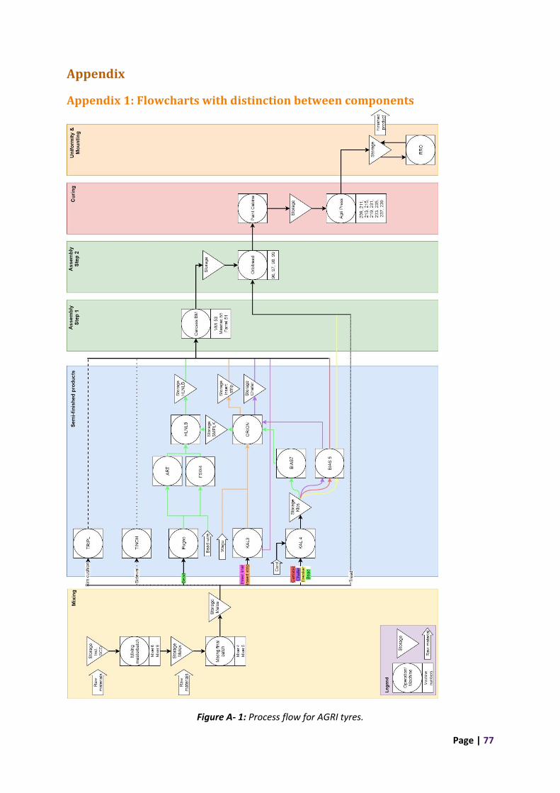
Page | 77
Appendix
Appendix 1: Flowcharts with distinction between components
Figure A- 1: Process flow for AGRI tyres.

Page | 78
Figure A- 2: Process flow for SM tyres.

Page | 79
Appendix 2: Dashboard to identify the bottleneck The dashboard is a tool that supports the first step of the TOC cycle: Identify the bottleneck. It shows
the information needed for the 4 phases of the bottleneck identification process and also indicates
some of the outcomes. The dashboard contains 6 pages. The first four pages form the bottleneck
identification process and page 5 and 6 give insight on the losses at the bottleneck. Thus, page 5 and
6 are part of the bottleneck analysis and give first insights to start step 2 of the TOC cycle: “optimize
the bottleneck”.
The first page “Bottleneck identification” is shown in Figure A- 3. In the upper left corner is a slicer
that can be used to filter on the date. Below, information is given about the definitions that are used.
Next, the tables for Phase 1-3 are given. The table for Phase 1 shows the machines with a GAP(%)>
50% in green, because they are identified as non-bottleneck machines. The machines identified as
non-bottlenecks are left out of the next tables. The second table for Phase 2 shows the machines
with TB+ST (%) < 2% in red, because they are identified as a potential bottleneck. The second and
third page also support Phase 2, these pages are explained later. The table for Phase 3 shows the
utilization per machine and the TB+ST (%) < 2%. This table is sorted on the utilization, which results in
the identification of the first machine (highest utilization) that has TB+ST (%) < 2% (which is indicated
in red) as the bottleneck. Finally, on the right there is a table that represents Phases 1 to 3. This table
gives an overview of the three phases per machine. One additional column, TS(%), is added to show
the division between TS and TB.
The second page “Visualization Phase 2” represents the visualization of Phase 2. This page is
represented in Figure 5.1 (Chapter 5). It shows the TB(%), TS(%) and TB-TS(%) per machine or
machine group in the flowchart. This results in the visibility of the principle of the turning point
method. It shows a rough pattern starting on the left with positive TBi − TSi, changing into a TBi −
TSi around zero and ending on the right in a negative TBi − TSi. This page is added to create
understanding of the method and its variables. In the upper left corner is a slicer that can be used to
filter on the date. Below the slicer is a table that (where possible) represents the TB and TS for
machines within a machine group. If one of the machine groups is the bottleneck, this table makes
the difference in TB and TS visible.
The third page “Caused starvation Phase 2” represents the second part of Phase 2 and is shown in
Figure 5.2 (Chapter 5). Here we see the minutes of starvation caused by the machine (instead of the
starvation at the machine). Again, the dashboard can be filtered on the preferred dates in the left
upper corner. This page is used to see the effect of the machine on succeeding processes. Combining
this page with the first page gives a conclusion on the location of the bottleneck (according to the
turning point method).
The fourth page “Information starvation” that is represented in Figure A- 4, is a page that is used as
input for page 3. This page is not directly needed to identify the bottleneck, but is handy to decide
how to adapt the figure when changes occur. It shows the reasons of starvation per station (and per
department). In combination with the flowcharts from chapter 3 we find out which machine has
caused the starvation. This is used to develop page 3. To include all possible relations this page shows
the data of one year. If changes occur and result in changes within the flow or starvation types, it can
be found in this page and accordingly altered in page 3.
Page | 80
The fifth page “Machine information” gives information about the bottleneck machine, see Figure A-
5. On the left side we can filter on the date, select the bottleneck machine and select the starvation
description caused by the bottleneck machine. The information in the upper left corner, within the
purple rectangle is fixed. The first graph shows the net production time (%) per week, which indicates
the occupation of the bottleneck machine over time. The second graph shows the total downtime
(Min) per week for the bottleneck machine. The third graph shows the starvation (Min) per week
caused by the bottleneck machine. These graphs provide information on the fluctuation at the
bottleneck machine. Also, we use these graphs to check if there is a relation.
The sixth page “Machine losses” gives information about the losses at the bottleneck machine, see
Figure A- 6. On the left side we can filter on date and select the bottleneck machine. Because the
graphs use two different data sets, we need to select the bottleneck machine twice. The graph in the
middle shows the top 5 tpm group losses (Min). The graph on the right shows the losses (Min) of the
possible down descriptions within the top 5 tpm groups. These figures give insight on the booked
losses at the bottleneck machine.
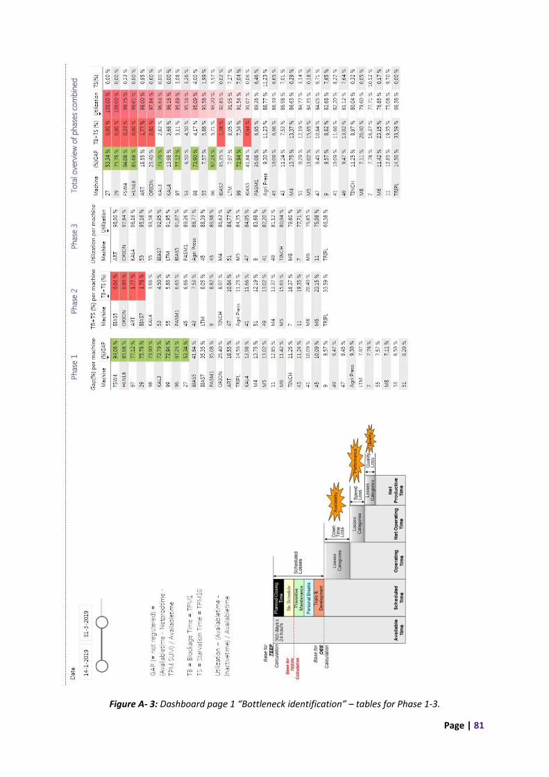
Page | 81
Figure A- 3: Dashboard page 1 “Bottleneck identification” – tables for Phase 1-3.
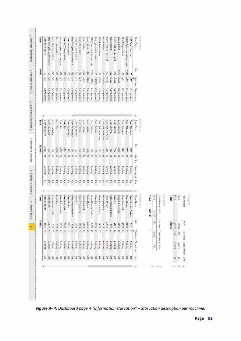
Page | 82
Figure A- 4: Dashboard page 4 “Information starvation” – Starvation description per machine.
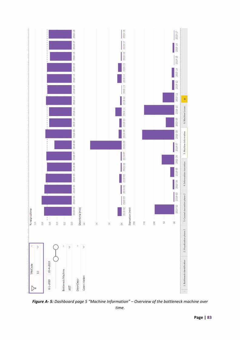
Page | 83
Figure A- 5: Dashboard page 5 “Machine Information” – Overview of the bottleneck machine over
time.
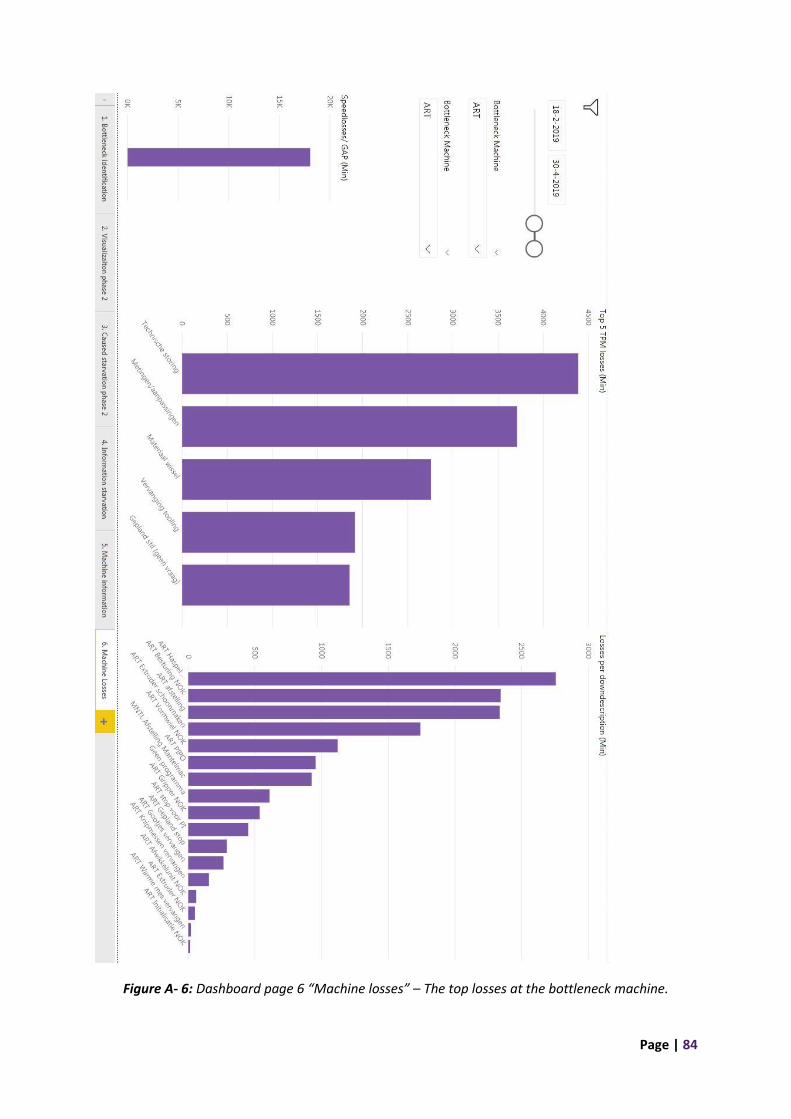
Page | 84
Figure A- 6: Dashboard page 6 “Machine losses” – The top losses at the bottleneck machine.

Page | 85
Appendix 3: Extensive descriptions of causes 1. The PIPO (Periodiek Inspectie Preventief Onderhoud) is planned far ahead. This means that
the PIPO can be scheduled in a time period that has an extraordinarily high workload. The
PIPO is planned far ahead because the schedule includes the entire plant. The impact of the
PIPO for the ART varies, because the load of the ART is irregular. There is only a small buffer
(safety lead time) to limit the impact, which makes the timing of the PIPO for the ART very
important.
2. Rush orders can cause additional changeover times. These rush orders occur because of last-
minute changes in demand or because the demand is not present in the planning. Last-
minute changes can occur in three situations. First, if planning is not followed, too many or
too few tyres for an order are made. Too few tyres affect the succeeding processes and too
many tyres affect the preceding processes. That means, if the building department produces
too many tyres for one order, they are using input materials that are not linked to that order
and thus reserved for another order. When that order needs to be produced, the material is
not available and this will result in a rush order. Second, a certain amount of greentyres is
rejected and becomes scrap. In the planning they estimate the amount of scrap, but in reality
the amount of scrap fluctuates. That means that the amount of greentyres produced is not
sufficient to fulfil the demand from the curing department. Depending on the order, a
decision is made to place a rush order to complete the order or to accept the loss at the
curing department. Third, the operators at the building department have a different level of
skill, which results in different building speeds. The planning uses a fixed speed for everyone.
Thus, operators can be faster than what is anticipated in the planning. If the difference is big
enough, it can occur that materials for the next order are not available yet. Again, a decision
is made to place a rush order to obtain the materials or to accept temporarily not being able
to produce. The sub-causes of different levels of skill of operators is described in cause 7.
Demand that is not present in the planning is caused by mistakes in the manual assessment
of the inventory. The impact of the rush orders is larger, because there is only a small buffer
of beads (based on the safety lead time) to deliver from.
3. The planning at the ART consists of small batches because they are linked to an order. The
planning manually combines orders if they think it is beneficial. Not only the finished bead is
linked to the order, but also the formed beads (without wrapping material) are already linked
to the order. Thus, the beads are made to order, which results in small batches.
4. The ART deals with an irregular load. Thus, the demand at the ART is fluctuating. A part of
this fluctuation is caused by fluctuations in demand for tyre types throughout the year.
Another part is caused by the division of agricultural beads specs on the ART and HVM4. The
planning department does not take this division into account while making the planning.
Thus, it can occur that one week most agricultural bead specs need to be produced on the
ART and the other week on the HVM4. This difference has a large impact on the load of the
ART.
5. The ART is a non-automatic machine. This means that a lot of the work is done manually and
requires a lot of time. This is caused by the machine being very old. This is a condition that
the process needs to deal with.
6. There is a large number of different bead specs resulting in many changeovers at the ART.
Vredestein offers a great variety of tyre types per product line, which increases the
complexity of the plant. This is one of the unique selling points of the plant and is also a
Page | 86
condition that the process needs to deal with. Also, all SM tyres and a part of the AGRI tyres
can only be processed on this machine. This means that the machine not only deals with
different tyre types within one product line, but within two. This increases the number of
specs.
7. The level of skill between operators can vary greatly. This impacts not only the working
speed, but also the way of working and dealing with defects. This is further described in
cause 8. The different levels of skill are mainly caused by the amount of training that
operators have had on the machine. Of course, the natural ability of an operator also
contributes to the level of skill. There is a great deviation in the amount of training, because
we work with temporary workers in addition to the permanent employees. Also, sometimes
employees from other machines or departments are used to support areas with a higher
workload.
8. Sometimes major failures occur at the engine. Often these defects occur as a result of small
defects not being noticed. An example includes the wire cutter. A small defect at the wire
cutter resulted in the wire not being completely cut through. Thus, the wire is teared loose
by the machine. Every time this happens, the engine must deliver more torque. After some
time, this results in a major failure at the engine. Skilled operators notice these defects. In
this case they notice the sound that is created by tearing the wire. Operators with a low level
of skills do not notice smaller defects that, in time, cause the major failures.
9. It is inevitable that the machine needs some preventive calibration. However, a lot of time is
lost with calibrations that can be prevented because they are a machine failure. Due to a bug
in the software, the wire cutter sometimes stops. After the bead is pulled down manually,
the wire cutter is not automatically activated. The machine needs to be calibrated to activate
the wire cutter.
10. A lot of time is spent fine-tuning the ART. Every operator starts his shift with fine-tuning the
machine according to his knowledge. This has two sub-causes: the possibility to fine-tune
and not having a standardized procedure. It is unclear what should be fine-tuned and what
the setting should be. This results in a different opinion per operator and thus continuous
fine-tuning between shifts.
11. The beads are formed around a shaping wheel. The beads of size 18 inch 16 strings need to
be removed manually from the shaping wheel, because the shaping form does not fold in
correctly. The shaping form does not fold in correctly, because the gripper does not grab this
size.
12. Uneven rubberization of steel wires. Uneven rubberization is caused by a clogged extruder.
The longer a clogged extruder stays unnoticed, the higher the impact. The camera placed
after the extruder is broken, which hinders the detection of uneven rubberization. Also,
uneven rubberization occurs more often at high speeds. A clogged extruder can be caused by
two things: low quality rubber or overdue cleaning. A low quality rubber pollutes the
extruder faster.
13. New safety issues are tackled throughout the factory. For the ART this led to temporary
safety locks. The temporary safety locks take more time compared to permanent safety
locks.
14. A spool of steel wire is replaced by hand. They used to do this with a carriage, but the
carriage is defect. The advantage of the carriage is that it can be prepared before replacing
Page | 87
the spools. Thus, the time to replace the wire and thus the time the machine stands still is a
little less with a carriage.
15. There are many defects expected to be caused by insufficient periodic maintenance. This is
caused by unclear relations between defects and responsibilities. There are two parties
involved with defects: the shift mechanic and technical service (day shift). They often point
to each other as the responsible person of that defect. This is caused by unclear division of
tasks.
16. There is a variation in rubber adhesion to the steel wire, because they use different qualities
of steel wire. The different qualities of wire come from three different suppliers.
17. No wrapping material in stock means that they cannot produce beads. A shortage of
wrapping material is caused by fluctuations. There are five situations that can cause
fluctuations. First, the rolls can contain different lengths of material, but there is always an
entire roll booked in the system. I.e. rolls that have the same SKU code can differ in size.
Also, no matter the size, an entire roll is booked in the system. Therefore, while there is
enough stock present in the inventory system, it might not be enough in practice. This leads
to material shortages. The material is order related meaning that all material booked in the
system is needed. The difference exists because the length of the roll (from the ORION) is not
booked. The length is mostly defined two processes prior, at KAL4. After KAL4 the “mother
roll” is cut at succeeding processes with a minimum amount of scrap and arrives as wrapping
material at the ART. None of these processes book the length of the roll. Second, shortages
can also occur when the production planning is not followed. This can be for both the
delivering and demanding process. If the delivering process does not follow planning,
delivery deadlines can be missed causing shortages. If the demanding process does not
follow planning, it is using material that is not accounted for. Thus, it is using material meant
for another order, which leads to shortages later on. The main reason for not following
planning is the KPIs that are used. Currently they steer on numbers produced, which means
that for instance postponing a set up to the next shift by producing more than planned is
beneficial for their KPIs. Third, the irregular demand at the ART causes overcapacity
sometimes, and under capacity at other times. If there is overcapacity they can build up
stock. This stock can grow over 8 hours, but the planning horizon does not go further than 8
hours. Even though they have no plan, they continue producing, because they know the
situation can easily shift. Thus, they start making beads with regular demand. These
production batches are discussed with the planning department and orders needed for input
materials are created. Because the ORION is also a machine with a high utilization and these
orders are added last-minute, the material often arrives too late, causing shortages. Note
that these shortages are only occurring if the machine is ahead of schedule and thus not the
most significant bottleneck at that point in time. Fourth, large defects at the ORION result in
shortages for its succeeding processes. This can also result in not delivering wrapping
material in time at the ART. Fifth, fluctuations that occur are not absorbed enough. The
current buffer is not sufficient to deliver from in case of unexpected changes, such as
fluctuations.
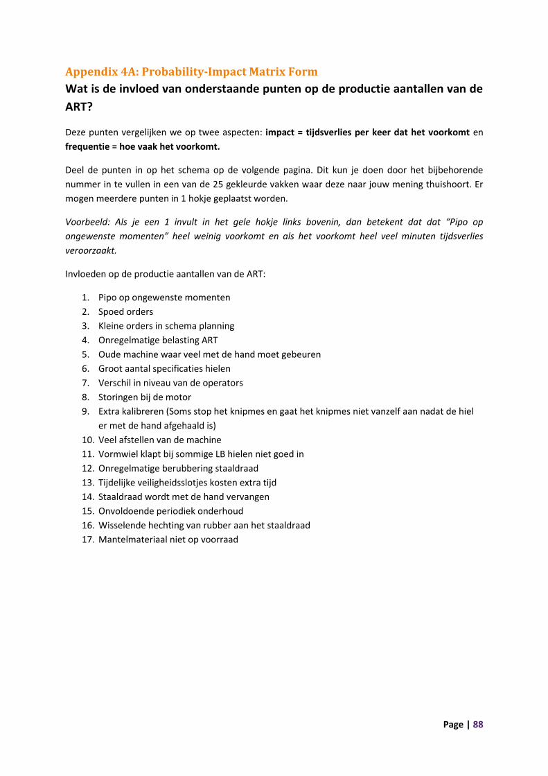
Page | 88
Appendix 4A: Probability-Impact Matrix Form
Wat is de invloed van onderstaande punten op de productie aantallen van de
ART?
Deze punten vergelijken we op twee aspecten: impact = tijdsverlies per keer dat het voorkomt en
frequentie = hoe vaak het voorkomt.
Deel de punten in op het schema op de volgende pagina. Dit kun je doen door het bijbehorende
nummer in te vullen in een van de 25 gekleurde vakken waar deze naar jouw mening thuishoort. Er
mogen meerdere punten in 1 hokje geplaatst worden.
Voorbeeld: Als je een 1 invult in het gele hokje links bovenin, dan betekent dat dat “Pipo op
ongewenste momenten” heel weinig voorkomt en als het voorkomt heel veel minuten tijdsverlies
veroorzaakt.
Invloeden op de productie aantallen van de ART:
1. Pipo op ongewenste momenten
2. Spoed orders
3. Kleine orders in schema planning
4. Onregelmatige belasting ART
5. Oude machine waar veel met de hand moet gebeuren
6. Groot aantal specificaties hielen
7. Verschil in niveau van de operators
8. Storingen bij de motor
9. Extra kalibreren (Soms stop het knipmes en gaat het knipmes niet vanzelf aan nadat de hiel
er met de hand afgehaald is)
10. Veel afstellen van de machine
11. Vormwiel klapt bij sommige LB hielen niet goed in
12. Onregelmatige berubbering staaldraad
13. Tijdelijke veiligheidsslotjes kosten extra tijd
14. Staaldraad wordt met de hand vervangen
15. Onvoldoende periodiek onderhoud
16. Wisselende hechting van rubber aan het staaldraad
17. Mantelmateriaal niet op voorraad
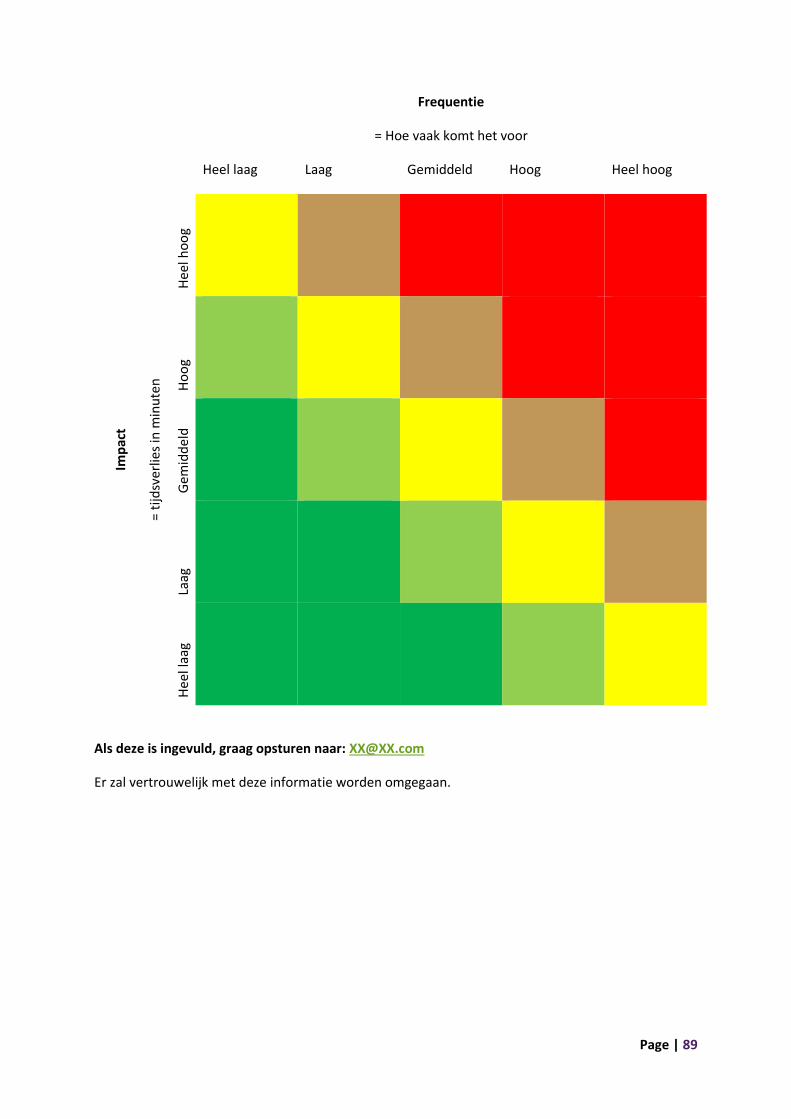
Page | 89
Frequentie
= Hoe vaak komt het voor
Heel laag Laag Gemiddeld Hoog Heel hoog
Imp
act
= t
ijdsv
erlie
s in
min
ute
n
Hee
l ho
og
Ho
og
Gem
idd
eld
Laag
Hee
l laa
g
Als deze is ingevuld, graag opsturen naar: [email protected]
Er zal vertrouwelijk met deze informatie worden omgegaan.
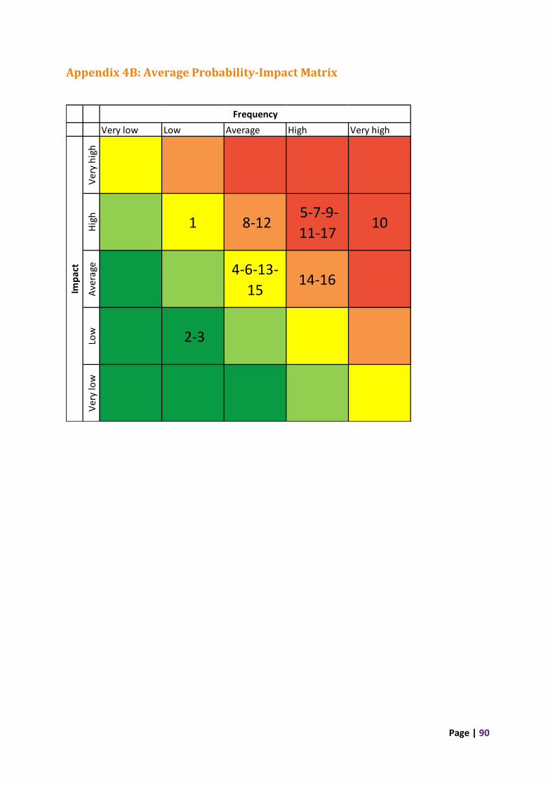
Page | 90
Appendix 4B: Average Probability-Impact Matrix
Very low Low Average High Very high
Ver
y h
igh
Hig
h
1 8-12 5-7-9-
11-1710
Ave
rage 4-6-13-
1514-16
Low 2-3
Ver
y lo
w
Imp
act
Frequency
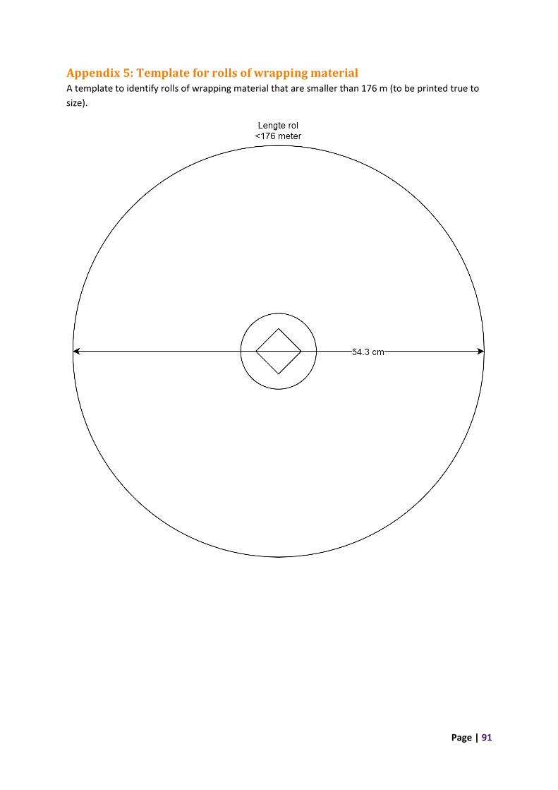
Page | 91
Appendix 5: Template for rolls of wrapping material A template to identify rolls of wrapping material that are smaller than 176 m (to be printed true to
size).