NREL is a national laboratory of the U.S. Department of Energy, Office of Energy Efficiency and Renewable Energy, operated by the Alliance for Sustainable Energy, LLC.

A Bottom-up Cost Analysis of a High Concentration PV Module

Kelsey A.W. Horowitz and Michael Woodhouse Strategic Energy Analysis Center Greg Smestad Sol Ideas Technology Development, Solar Energy Materials and Solar Cells Journal Hohyun Lee University of Santa Clara

Alfred Hicks and Kendra Palmer Graphics and Communications

NREL/PR-6A20-63947

CPV-11 Aix-les-Baines, France 13-15 April 2015

2

Analysis Disclaimer DISCLAIMER AGREEMENT These manufacturing cost model results (“Data”) are provided by the National Renewable Energy Laboratory (“NREL”), which is operated by the Alliance for Sustainable Energy LLC (“Alliance”) for the U.S. Department of Energy (the “DOE”). It is recognized that disclosure of these Data is provided under the following conditions and warnings: (1) these Data have been prepared for reference purposes only; (2) these Data consist of forecasts, estimates or assumptions made on a best-efforts basis, based upon present expectations; and (3) these Data were prepared with existing information and are subject to change without notice. The names DOE/NREL/ALLIANCE shall not be used in any representation, advertising, publicity or other manner whatsoever to endorse or promote any entity that adopts or uses these Data. DOE/NREL/ALLIANCE shall not provide any support, consulting, training or assistance of any kind with regard to the use of these Data or any updates, revisions or new versions of these Data. YOU AGREE TO INDEMNIFY DOE/NREL/ALLIANCE, AND ITS AFFILIATES, OFFICERS, AGENTS, AND EMPLOYEES AGAINST ANY CLAIM OR DEMAND, INCLUDING REASONABLE ATTORNEYS' FEES, RELATED TO YOUR USE, RELIANCE, OR ADOPTION OF THESE DATA FOR ANY PURPOSE WHATSOEVER. THESE DATA ARE PROVIDED BY DOE/NREL/ALLIANCE "AS IS" AND ANY EXPRESS OR IMPLIED WARRANTIES, INCLUDING BUT NOT LIMITED TO, THE IMPLIED WARRANTIES OF MERCHANTABILITY AND FITNESS FOR A PARTICULAR PURPOSE ARE EXPRESSLY DISCLAIMED. IN NO EVENT SHALL DOE/NREL/ALLIANCE BE LIABLE FOR ANY SPECIAL, INDIRECT OR CONSEQUENTIAL DAMAGES OR ANY DAMAGES WHATSOEVER, INCLUDING BUT NOT LIMITED TO CLAIMS ASSOCIATED WITH THE LOSS OF DATA OR PROFITS, WHICH MAY RESULT FROM AN ACTION IN CONTRACT, NEGLIGENCE OR OTHER TORTIOUS CLAIM THAT ARISES OUT OF OR IN CONNECTION WITH THE USE OR PERFORMANCE OF THESE DATA.

3

Acknowledgments

Al Hicks Kendra Palmer Dr. Sarah Kurtz Dr. Dan Friedman All our collaborators in industry

SEAC management team for helpful reviews of this work

Dr. Michael Woodhouse Dr. Greg Smestad Dr. Hohyun Lee

Co-authors

4

Executive Summary • We have created a bottom-up cost model for analyzing III-V

multi-junction cells and HCPV modules • There are several avenues to reduced cell manufacturing costs:

o Largest drivers are scale, manufacturing yield, and substrate reuse o Metallization costs, III-V deposition rates, and precursor prices are

also important contributors • Many different components (cell, structure, receiver board,

thermal management) contribute significantly to cost and represent opportunities for cost reduction, although performance trade-offs must always be considered.

• Increases in cell efficiency and reduction in cell costs represent significant opportunity for module cost reductions across many designs

• The ultimate competitiveness of HCPV must be determined with a complete systems and LCOE analysis, which we are currently undertaking

5

Motivation: Changing Flat-plate PV Prices What is the value proposition of CPV today now that traditional, flat-plate PV prices have plummeted?

2012

Reductions in the German FiT begin

Representative manufacturing costs roadmap

Module Price Sources: Navigant and UBS consulting services

6

Motivation: Efficiency • High efficiencies of III-V cells (purple) could allow for significant future

module and system cost reductions for HCPV • Efficiency is a lever for decreasing module costs, system costs, and LCOE

7

Motivation: Low Reported Costs CPV has reported system costs within the range of traditional, flat-plate PV at much lower volumes.

Haysom, J.E.; Jafarieh, O.; Anis, H.; Hinzer, K.; Wright, D. (2013). “Learning curve analysis of concentrated photovoltaic systems.” Prog. Photovolt: Res. Appl. 1556: 239.

8

Motivation: Bankability and Scale The struggles of the CPV market, combined with the higher complexity of the technology, lack of standardization, and small number of installations, may present barriers for obtaining the funding necessary to scale and reduce costs

From “Chicken or the egg.” (2015). Accessed March 2015: http://en.wikipedia.org/wiki/Chicken_or_the_egg.

NREL image gallery 13735, 13740, 18303

9

Analysis Objective

Calculate the $/Wp costs of a model HCPV module and III-V multi-junction cells

o Provide an understanding of where HCPV costs are and could be with current technology if manufacturing was scaled up

o Illuminate the cost drivers for this technology, as well as potential pathways for future cost reductions

– Understand potential challenges in achieving these cost reductions

o Set the stage for future levelized cost of energy (LCOE) calculations.

10

Manufacturing Cost Analysis Methodology

Methods • Bottom-up calculation where we

compute: o Materials o Utilities o Labor o Depreciation o Maintenance

costs associated with each step in the manufacturing process • Input data sourced from multiple

material suppliers and equipment vendors

• Results reviewed by industry members and NREL experts who provide feedback to improve and validate the model.

Assumptions • Manufacturing in low-cost region

of the United States • Annual production volumes:

o For cells: 50 MW and 0.1 MW (at one sun)

o For modules: 100 MW • Depreciation schedules:

o 5-year and 7-year straight-line for cell and module equipment, respectively

o 15-year straight-line for buildings.

11

Minimum Sustainable Price (MSP) • MSP: The price at which the net present value (NPV) of a 20-year project is equal

to zero o Minimum price required to generate a required rate of return o We set the required rate of return to be the weighted average cost of capital (WACC)

– E = % equity, D = % debt, re = cost of equity, rd = cost of debt, rt = corporate tax rate – WACC = 15% calculated for the U.S. PV market in 2014 – More information in: Fu, Ran et al. “Economic Measurements of Polysilicon for the

Photovoltaic Industry: Market Competition and Manufacturing Competitiveness,” IEEE JPV 5, pp. 515-524 (2015) http://ieeexplore.ieee.org/xpl/articleDetails.jsp?arnumber=7042229

• Included in the NPV calculation: o Manufacturing costs o Overhead costs

– Research and development (R&D) costs, assumed to be 8% of revenue – Sales, general and administrative (SG&A) costs, assumed to be 4% of revenue – Other costs (warranty, legal) assumed to be 2% of revenue

o Taxes, 28% effective federal corporate tax rate assumed o Zero salvage value

12

Model Triple Junction III-V Cell • This type of cell is currently the most commonly used by the HCPV industry, but several different

triple junction III-V cell designs are commercially available.

• Details on the manufacturing process for III-V cells can be found in: Woodhouse, M.; Goodrich, A. (2014). “Manufacturing Cost Analysis Relevant to Single-and Dual-Junction Photovoltaic Cells Fabricated with III-Vs and III-Vs Grown on Czochralski Silicon.” NREL/PR-6A20-60126. Golden, CO: NREL. http://www.nrel.gov/docs/fy14osti/60126.pdf

13

III-V Multi-junction Cell Cost Drivers Biggest cost drivers:

o Ge substrate ($150/6’’ wafer) o Low manufacturing yield (80% assumed here) o Metallization (Au and Ag targets, low material utilization) o Base layers (expensive precursors, slow deposition).

14

Cell Cost Sensitivity Analysis Sensitivity of Cell Costs to a ± 25% Change in Input Parameter

• Current manufacturing yields for III-V multi-junctions: 75%-85%, 80% used for our reference case

• Note this sensitivity is itself sensitive to the initial design • This also not reflective of the magnitude of changes that might be

technically possible

15

Cost Reduction Roadmap

• Increased material utilization and deposition rates estimated for maintaining material quality • Currently, only 5-10 substrate reuses have been publically demonstrated • No currently known methods for achieving a high number of reuses of the Ge substrate. It’s

not clear how this could be accomplished at scale, or what additional layers would need to be grown. Thus this may not even be feasible at scale or for large numbers of reuses, or could add costs beyond what is shown here. NREL has ongoing work to investigate these issues.

No public demonstrations to date

No wafer reuse assumed in the reference case. For 50MW/year 1 sun equivalent production capacity

16

Impact of Substrate Reuse

• For reference case parameters • Diminishing returns after 50 substrate reuses • Again, the additional processing steps or layer growth required to

achieve a substrate reuse at scale is currently unknown, so the estimates of costs with many substrate reuses are likely low.

17

Costs at Concentration

• Φs = cell costs in $/m2 • Φx = primary optic costs in $/m2 • C = effective (or optical) concentration ratio • ηx = throughput efficiency of the concentrator • ηs =cell efficiency • Px = 1,000 W/m2 and corresponds to the CSTC incident DNI solar

resource. Fahrenbruch, A.L.; Bube, R.H. (1983). “Concentrators, Concentrator Systems, and Photoelectrochemical Cells.” Fundamentals of Solar Cells Photovoltaic Solar Energy Conversion. Elsevier.

18  

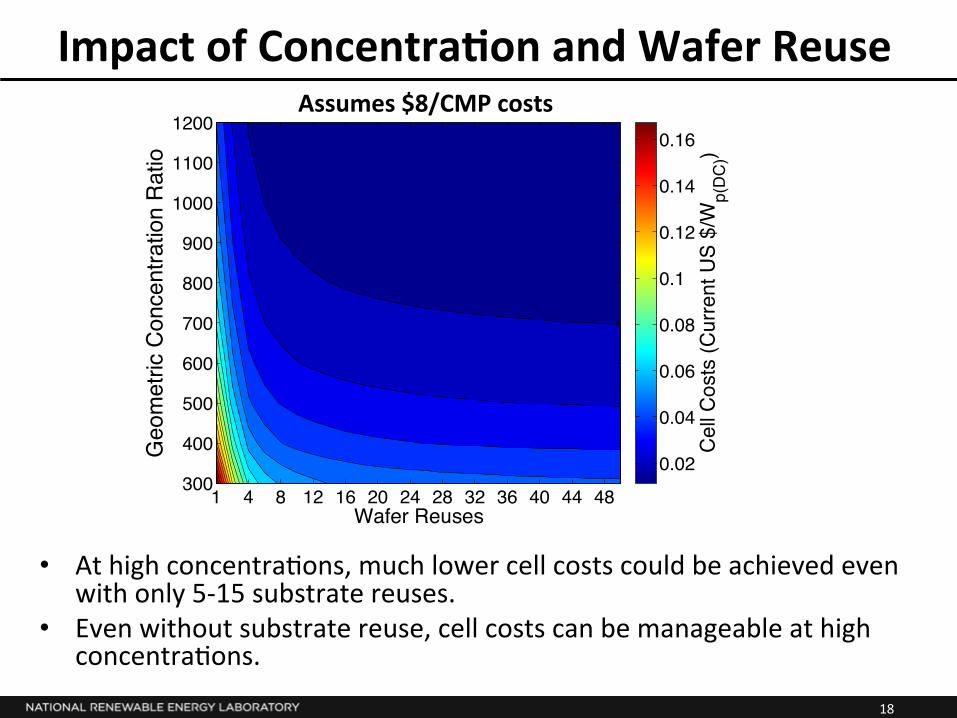
Impact  of  Concentra9on  and  Wafer  Reuse  Assumes  $8/CMP  costs  

Wafer Reuses

Geo

met

ric C

once

ntra

tion

Rat

io

1 4 8 12 16 20 24 28 32 36 40 44 48300

400

500

600

700

800

900

1000

1100

1200

Cel

l Cos

ts (C

urre

nt U

S $/

Wp(

DC

))

0.02

0.04

0.06

0.08

0.1

0.12

0.14

0.16

•  At  high  concentra*ons,  much  lower  cell  costs  could  be  achieved  even  with  only  5-­‐15  substrate  reuses.    

•  Even  without  substrate  reuse,  cell  costs  can  be  manageable  at  high  concentra*ons.    

19

Model Module Design

While this model is certainly not representative of the entire HCPV space, which includes a wide variety of designs, it contains the same fundamental elements as many commercial modules.

Reference Design • 1,000x geometric

concentration • 30% module efficiency • Silicone-on-glass (SOG)

Fresnel lens primary • Dome secondary lens • 5mm x 5mm

Ge/Ga(In)As/GaInP cells • 50 cells/module • Rectangular box housing • Passive thermal

management via an aluminum plate.

20

Manufacturing Process Flow Injection molding is more typical for PMMA lenses.

21

Step-by-step Module Manufacturing Costs

Many pieces contribute to cost (cells, optics, housing, receiver board, and thermal management)

22  

Impact  of  Concentra9on  and  Efficiency  

•  Concentra*on  ra*o  and  cell  efficiency  are  coupled  •  At  higher  concentra*ons,  addi*onal  thermal  management  will  be  required  •  This  curve  is  only  relevant  for  this  specific  module  design.  

26 28 30 32 34 36 38 40 42 44 46 48 50300

400

500

600

700

800

900

1000

1100

1200

Cell Efficiency

Geo

met

ric C

once

ntra

tion

Rat

io

Mod

ule

Cos

ts (C

urre

nt U

S $/

Wp(

DC

))

0.4

0.6

0.8

1

1.2

1.4

1.6

23

Potential Pathways to Reduced Cost

• Many areas for cost reduction • Will need reductions in many component costs in $/m2, or increase in efficiency to achieve

dramatic cost reductions • Performance-cost trade-offs and technical feasibility of these cost reductions must be explored in

more detail. o It may not be possible to achieve all of these improvements and maintain performance. o Improving cell efficiency will likely increase $/m2 cell costs. But scale and manufacturing learning

could help reduce cell $/m2 costs while maintaining or improving efficiency. o Alternative designs may be able to achieve additional cost reductions, this just gives an example.

$0.77/Wp(DC)

$0.29/Wp(DC)

24

Impact of Efficiency on Module Costs

Module Efficiency = (Cell Efficiency)*(Throughput Efficiency) Throughput efficiency considers optical efficiency and acceptance angle.

Reference Case Module Efficiency

25

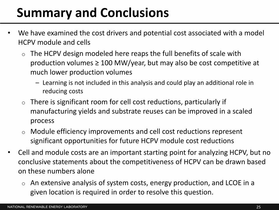
Summary and Conclusions • We have examined the cost drivers and potential cost associated with a model

HCPV module and cells o The HCPV design modeled here reaps the full benefits of scale with

production volumes ≥ 100 MW/year, but may also be cost competitive at much lower production volumes

– Learning is not included in this analysis and could play an additional role in reducing costs

o There is significant room for cell cost reductions, particularly if manufacturing yields and substrate reuses can be improved in a scaled process

o Module efficiency improvements and cell cost reductions represent significant opportunities for future HCPV module cost reductions

• Cell and module costs are an important starting point for analyzing HCPV, but no conclusive statements about the competitiveness of HCPV can be drawn based on these numbers alone o An extensive analysis of system costs, energy production, and LCOE in a

given location is required in order to resolve this question.

26

Thank you!

Kelsey.Horowitz@nrel.gov

We are always interested in collaborating with industry, other national labs, or universities!

27

Back-up Slides

28

Thermal Management Modeling

29

Thermal Management: Methods • Simulations of thermal management requirements were performed in conjunction with Dr. Hohyun

Lee of Santa Clara University. • The simulations incorporated the geometries shown here. The model was a simplification, with the

following were not included: o Detailed assumptions about the geometry of the copper traces o The effect of the bypass diode o The effect of structural supports or module housing o Thus, thermal management requirements may be slightly overestimated

• We compared thermal management solutions with Al2O3, SiNx, and AlN ceramic boards with assumed thermal conductivities of 25 W/mK, 90 W/mK, and 180 W/mK, respectively.

• Aluminum volumes required to maintain temperatures below 353 K were computed via thermal modeling and then used to compute materials costs, assuming an aluminum price of $2.2/kg. Processing costs were determined by consultation with heat sink vendors.

Side view of the simulated geometry without fins.

Layer Thermal Conductivity (W/mK)

Thickness (mm)

III-V multi-junction cell 60 0.205

Copper 285 0.2

Ceramic board varied varied

Aluminum plate 205 3

Input Assumptions to the Thermal Model

30

Total Thermal Resistance

The thermal resistances of the aluminum heat sink and ceramic board will add up to determine the effectiveness of heat dissipation. Depending on the range of thermal resistance, 30% reduction in thermal resistance can easily double the required volume of the heat sink.

31

Thermal Management Results • The figure below assumes a ceramic plate of thermal conductivity 90 W/mK. Results

are similar with a 180 W/mK ceramic plate. • This analysis illustrates that a 3mm thick aluminum plate is sufficient to maintain cell

temperatures below 353K for a wide range of concentrations in a point-focus system. • At scale, a significant difference in the cost of AlN and SiNx plates is not expected.

Ceff is the effective concentration corresponding to the amount of thermal energy the thermal management system is required to dissipate. For the plot shown at the left, we assume 41% cell efficiency and 85% optical efficiency Cg = Ceff/0.426

32

Energy Production Issues

33

Energy Production Limitations on energy production in CPV modules (true for both LCPV and HCPV)

o System Efficiency o Solar Resource, in terms of location, spectrum,

season, time of day o Other Qualities of Solar Resource, such as the

angular spread of the sunlight and whether or not the resource is direct or diffuse

o Angular Response of the Module, determined by the optical design, module alignment, temperature, mechanical stress on the optics

o Tracker Error/Accuracy, determined by the tracker slew drive, controller, and module support structure.

Also a factor for flat-plate modules

Unique to CPV

34

Acceptance Angle • Acceptance angle is always a function of concentration, with lower concentrations

having a larger acceptance angle. • However, acceptance angle is also a function of the optical design, and so there can

be a higher concentration design with the same acceptance angle as a lower concentration design with different optics, as shown in the example below.

The acceptance angle for ideal concentrator, i.e., the theoretical maximum acceptance angle, is determined by the following relationship: C = n2/sin2θ

C = concentration ratio < Cg θ = acceptance angle n = refractive index

35

How Does this Translate to Efficiency?

• Efficiency lost due to acceptance angle limitations and tracker errors will depend on the specific module response curve

• There is currently no standard definition of acceptance angle. People use 90%, 95%, and 98% acceptance angles in the literature, with 90% being the most common

• Just stating an acceptance angle does not paint the full picture of expected energy production changes o Notably, if tracker or alignment errors are either large to begin with or larger than expected

(due to high wind, optical misalignment developing as a result of refractive index change or mechanical flexing of the optics, etc.), the energy production could actually be much less.

+α° -α° -2.5° +2.5° 0°

100% 90%

Loss with perfect tracking

Angular spread of DNI resource measured by pyrheliometers (±2.5°)

Tracking error (°)

Module response curve with some positive tracking

error

% o

f max

pow

er

prod

uctio

n

36

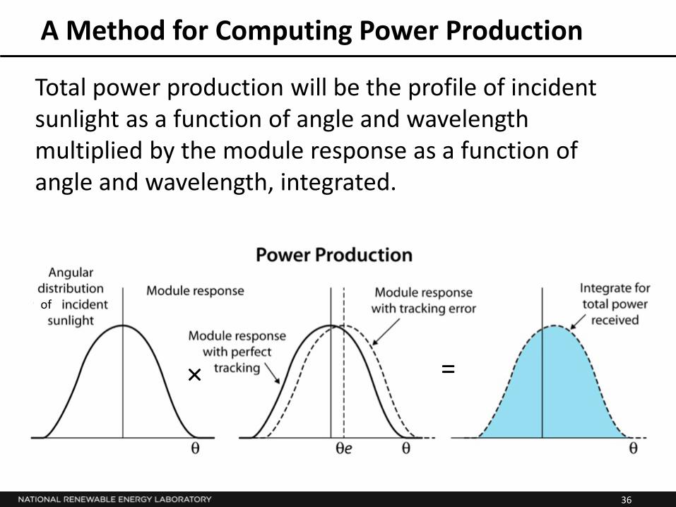
A Method for Computing Power Production

Total power production will be the profile of incident sunlight as a function of angle and wavelength multiplied by the module response as a function of angle and wavelength, integrated.

× =

of

37

Energy Production • Because of the complexity in CPV, and the lack of complete

understanding of the DNI resource, it is difficult to correctly model energy production.

• Thus, there is not a fully developed understanding of how much module energy production can vary with location, time of year, and module design. o This includes issues like impact of wind load on tracker error, effects of

soiling for different module designs, etc. o This also includes uncertainty in the spectral response of different III-V

multi-junction cells, which is the subject of current research efforts.

• This information also is essential to correctly determining the LCOE advantage (or disadvantage) of HCPV compared to flat-plate PV and tracked flat-plate PV in different locations for different modules.

• Some published studies on HCPV system energy production, measured and modeled, are listed in the note. This is an active area of study.

38

References on Energy Production

Kurtz, Sarah et al. Key parameters in determining energy generated by CPV modules. Prog. Photovolt: Res. Appl. (2014) Gomez-Gil, Francisco, et al. Analysis and Prediction of Energy Production in Concentrating Photovoltaic (CPV) Installations. Energies (2012), 5, 770-789 Liu, Mingguo et al. Performance Analysis and Modeling of the World’s Largest CPV Power Plant. 39th IEEE Photovoltaic Specialists Conference (PVSC), 1749 – 1754, 16-21 June 2013. Kinsey, Geoggrey et al. Energy prediction of Amonix CPV solar power plans. Prog. Photovolt: Res. Appl., 794-796 (2011) King, C. Site Data Analysis of CPV Plants. 35th IEEE PVSC, 3043-3047, 20-25 June 2010, Honolulu, HI.

39

Energy Production Recent work by Kurtz et al. (2014) has shed light on some issues related to energy production in several CPV modules.

o This data was taken in Golden, CO. For many regions where CPV may be deployed, the difference between winter and summer months is expected to be much smaller.

o While the trends are linear, there is not an exactly linear relationship between performance ratio and acceptance angle as there is also dependence on specific module design.

Each dot represents a different module that was measured.

40

Integral of Solar Input vs. angle

X CPV Throughput vs. input angle

dθ = actual DNI into concentrator system

41

Px vs. Angle

If the sky is hazy, then more of the radiation is farther out at larger angles.

42

Input Assumptions

43

Backup: Manufacturing Assumptions Made in Calculating Cell Costs

44

Backup: Input Parameters for the Reference Case HCPV Module

45

Converting Costs to $/W at Concentration

46

Cg = Cmax= Aaperture/Asolar cell = Ax/As

• Concentration is the process by which light from a larger area, Ax, is directed to a smaller area, As.

• The throughput efficiency describes the losses in that process and it can be called the total optical efficiency. Ceffective is the ratio of the optical power density at the solar cell to that at the concentrator entrance aperture.

• Power density (or irradiance) is measured in W/m2.

• Cg > Ceffective.

• Ceffective = Cg times throughput efficiency = Cg ηx.

Concentration Ratio

47

• C = PS/Px • The module efficiency is the product of the cell and

throughput efficiencies, so that ηmodCg= ηSC • Cg is the geometric concentration • C is the effective (or optical) concentration ratio • ηx is the throughput efficiency of the concentrator • ηs is the cell efficiency • Px is 1,000 W/m2 and corresponds to the CSTC incident DNI

solar resource. IEC. (2013). “IEC 62670-1 ed1.0. Photovoltaic concentrators (CPV) – Performance testing – Part 1: Standard Conditions.”

Notes on the Equation for Computing $/W at Concentration

48

Cost Equations: Step 1

Source: Fahrenbruch, A.L.; Bube, R.H. (1983). Fundamentals of Solar Cells Photovoltaic Solar Energy Conversion. Elsevier.

For this discussion, let’s take Ceffective = C

A is an Area ηx is the concentrator throughput efficiency

Px = incident solar power density C = ηxAx/As

C = Ps/Px = optical power density seen by the solar cell divided by the incident un-concentrated solar (optical) power density

49

Cost Equations: Step 2

Power Output = ηsAsPs = ηsηxAxPx ηs = conversion efficiency of solar cells

Source: Fahrenbruch, A.L.; Bube, R.H. (1983). Fundamentals of Solar Cells Photovoltaic Solar Energy Conversion. Elsevier.

All diagrams were drawn by Al Hicks, NREL.

50

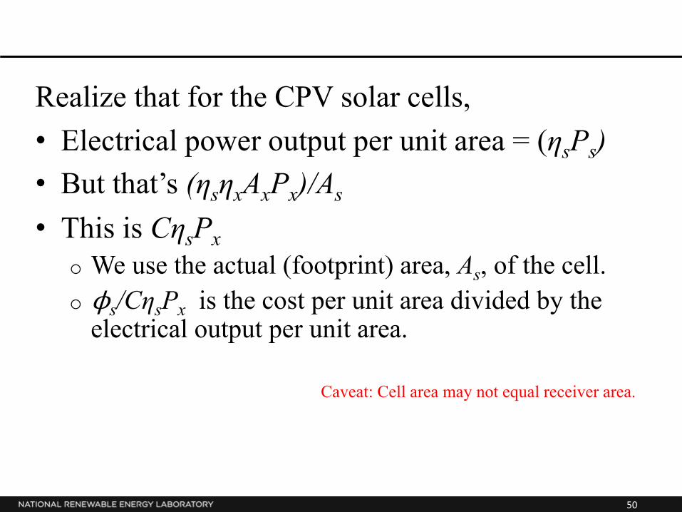
Realize that for the CPV solar cells, • Electrical power output per unit area = (ηsPs) • But that’s (ηsηxAxPx)/As • This is CηsPx

o We use the actual (footprint) area, As, of the cell. o ϕs/CηsPx is the cost per unit area divided by the

electrical output per unit area.

Caveat: Cell area may not equal receiver area.

51

Cost Equations: Step 3

Cost per unit area of the solar cell = ϕs Cost per unit area of the concentrator = ϕx

cost/area power output/area 1 ηsPx Source: Fahrenbruch, A.L.; Bube, R.H. (1983). Fundamentals of Solar Cells Photovoltaic Solar Energy Conversion. Elsevier.

= ϕs/CηsPx + ϕx/ηsηxPx $/Wp =

[ϕs/C + ϕx/ηx]

52

Energy Production Issues

53

We do not always have the same energy in the same solid angle.

All diagrams were drawn by Al Hicks, NREL.

54

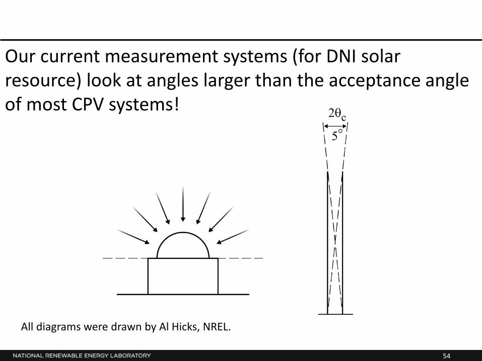
Our current measurement systems (for DNI solar resource) look at angles larger than the acceptance angle of most CPV systems!

All diagrams were drawn by Al Hicks, NREL.

55

Different concentrators have different acceptance angles.

All diagrams were drawn by Al Hicks, NREL.

56

CPV Energy Capture

57

Deep-dive into cost breakdowns

58

Breakdown of Module Housing Costs by Type

Assumes $3.2/kg steel costs (include materials costs and cost to manufacture housing pieces), $20/kg adhesive costs

59

Breakdown of Receiver Board Costs

Receiver board From “Concentrated photovoltaics.” (2015). Accessed March 2015: http://en.wikipedia.org/wiki/Concentrated_photovoltaics.