A Bregman extension of quasi-Newton updates I: an information geometrical framework

This article was downloaded by: [Harvard College]On: 27 April 2013, At: 08:07Publisher: Taylor & FrancisInforma Ltd Registered in England and Wales Registered Number: 1072954 Registeredoffice: Mortimer House, 37-41 Mortimer Street, London W1T 3JH, UK

Optimization Methods and SoftwarePublication details, including instructions for authors andsubscription information:http://www.tandfonline.com/loi/goms20

A Bregman extension of quasi-Newtonupdates I: an information geometricalframeworkTakafumi Kanamori a & Atsumi Ohara ba Department of Computer Science and Mathematical Informatics,Nagoya University, Furocho, Chikusaku, Nagoya, 464-8603, Japanb Department of Electrical and Electronics Engineering, Universityof Fukui, 3-9-1 Bunkyo, Fukui, 910-8507, JapanVersion of record first published: 04 Oct 2011.

To cite this article: Takafumi Kanamori & Atsumi Ohara (2013): A Bregman extension of quasi-Newton updates I: an information geometrical framework, Optimization Methods and Software,28:1, 96-123

To link to this article: http://dx.doi.org/10.1080/10556788.2011.613073

PLEASE SCROLL DOWN FOR ARTICLE

Full terms and conditions of use: http://www.tandfonline.com/page/terms-and-conditions

This article may be used for research, teaching, and private study purposes. Anysubstantial or systematic reproduction, redistribution, reselling, loan, sub-licensing,systematic supply, or distribution in any form to anyone is expressly forbidden.

The publisher does not give any warranty express or implied or make any representationthat the contents will be complete or accurate or up to date. The accuracy of anyinstructions, formulae, and drug doses should be independently verified with primarysources. The publisher shall not be liable for any loss, actions, claims, proceedings,demand, or costs or damages whatsoever or howsoever caused arising directly orindirectly in connection with or arising out of the use of this material.

http://www.tandfonline.com/loi/goms20

http://dx.doi.org/10.1080/10556788.2011.613073

http://www.tandfonline.com/page/terms-and-conditions

Optimization Methods & SoftwareVol. 28, No. 1, February 2013, 96–123

A Bregman extension of quasi-Newton updates I: an informationgeometrical framework

Takafumi Kanamoria* and Atsumi Oharab

aDepartment of Computer Science and Mathematical Informatics, Nagoya University, Furocho,Chikusaku, Nagoya 464-8603, Japan; bDepartment of Electrical and Electronics Engineering,

University of Fukui, 3-9-1 Bunkyo, Fukui 910-8507, Japan

(Received 22 November 2010; final version received 3 August 2011)

We study quasi-Newton methods from the viewpoint of information geometry. Fletcher has studied a vari-ational problem which derives approximate Hessian update formulae of quasi-Newton methods. We pointout that the variational problem is identical to the optimization of the Kullback–Leibler (KL) divergence,which is a discrepancy measure between two probability distributions. The KL-divergence introduces adifferential geometrical structure on the set of positive-definite matrices, and the geometric view helps ourintuitive understanding of the Hessian update in quasi-Newton methods. Then, we introduce the Bregmandivergence as an extension of the KL-divergence. As well as the KL-divergence, the Bregman diver-gence introduces the information geometrical structure on the set of positive-definite matrices. We deriveextended quasi-Newton update formulae based on the variational problem of the Bregman divergence.From the geometrical viewpoint, we study the invariance property of Hessian update formulae. We alsopropose an extension of the sparse quasi-Newton update. Especially, we point out that the sparse quasi-Newton method is closely related to statistical algorithm such as em-algorithm and boosting. We show thatthe information geometry is a useful tool not only to better understand the numerical algorithm but also todesign new update formulae in quasi-Newton methods.

Keywords: quasi-Newton method; information geometry; Bregman divergence

1. Introduction

The main purpose of this article is to propose an extension of quasi-Newton methods and toinvestigate the property of the numerical algorithm from the view point of the information geom-etry [2,30,36]. The quasi-Newton method is regarded as one of the most popular variable metricmethods in numerical optimization. Since Davidon had proposed the Davidon–Fletcher–Powell(DFP) update formula [10], many variable metric methods have been proposed. Nowadays, theBroyden–Fletcher–Goldfarb–Shanno (BFGS) method is considered to be the most effective inpractice. Indeed, the BFGS method has some interesting properties such as the self-correctingproperty for the inference of the Hessian matrix [32]. The research to discover more efficientvariable metric methods, however, has been going on intensively. The present paper also attempts

*Corresponding author. Email [email protected]

ISSN 1055-6788 print/ISSN 1029-4937 online© 2013 Taylor & Francishttp://dx.doi.org/10.1080/10556788.2011.613073http://www.tandfonline.com

Opt

imiz

atio

n M

etho

ds a

nd S

oftw

are

2013

.28:

96-1

23.

Optimization Methods & Software 97

to seek an efficient quasi-Newton method. As the first step, we extend the existing methods basedon the variational approach. Then, we provide an information geometrical view which will helpto better understand the belabour of the numerical optimization algorithm.

For large-scale problems, however, even the BFGS method is not effective, since storing thefull approximate Hessian matrix is required. To overcome this difficulty, several methods such asthe limited-memory BFGS (L-BFGS) method [31] and sparse quasi-Newton methods [15,40,41]have been proposed. In sparse quasi-Newton methods, the approximate Hessian matrix is keptsparse during the optimization procedure. We present that the sparse quasi-Newton method is alsowell understood based on the information geometry. Then, we propose an extension of the sparsequasi-Newton method.

Let us consider the unconstrained optimization problem

minimize f (x), x ∈ Rn, (1)

in which the function f : Rn → R is twice continuously differentiable on R

n. In quasi-Newtonmethods, a sequence {xk}∞k=0 ⊂ R

n is successively generated in the manner such that

xk+1 = xk − αkB−1k ∇f (xk).

The coefficient αk is the step length computed by a line search technique, and the matrix Bk is asymmetric positive-definite matrix which is expected to approximate the Hessian matrix ∇2f (xk).The matrix Bk and the step length αk are designed such that the sequence xk converges to alocal minima of the problem (1). The Wolfe condition [33, Section 3.1] is a standard criterion todetermine the step length αk . In terms of the approximate Hessian matrix, mainly there are twomethods of updating Bk to Bk+1: the DFP formula and the BFGS formula.

We briefly introduce the DFP and the BFGS methods. Let sk and yk be the column vectorsdefined by

sk = xk+1 − xk = −αkB−1k ∇f (xk), yk = ∇f (xk+1) − ∇f (xk),

and suppose that s�k yk > 0 holds. The condition s�

k yk > 0 is satisfied if the Wolfe condition isimposed on the line search. In the DFP formula, the approximate Hessian matrix Bk is updatedsuch that

Bk+1 = BDFP[Bk; sk , yk] := Bk − Bksky�k + yks�

k Bk

s�k yk

+ s�k Bksk

yky�k

(s�k yk)2

+ yky�k

s�k yk

. (2)

In the BFGS update formula, the matrix Bk+1 is defined by

Bk+1 = BBFGS[Bk; sk , yk] := Bk − Bksks�k Bk

s�k Bksk

+ yky�k

s�k yk

. (3)

If there is no confusion, the update formulae BDFP[B; s, y] and BBFGS[B; s, y] are written as BDFP[B]and BBFGS[B], respectively. Suppose that Bk be an n × n symmetric positive-definite matrix ands�

k yk > 0. Then, the matrices BDFP[Bk; sk , yk] and BBFGS[Bk; sk , yk] are also symmetric positive-definite matrices. In practice, the Cholesky decomposition of Bk is successively updated in orderto compute the search direction −B−1

k ∇f (xk) efficiently [18]. Note that the equality

BDFP[B; s, y]−1 = BBFGS[B−1; y, s]holds. Hence, we can derive the update formulae for the inverse Hk = B−1

k without the inver-sion of matrix, that is, we obtain Hk+1 = BBFGS[Hk; yk , sk] for the DFP update and Hk+1 =BDFP[Hk; yk , sk] for the BFGS update.

Opt

imiz

atio

n M

etho

ds a

nd S

oftw

are

2013

.28:

96-1

23.

98 T. Kanamori and A. Ohara

Both the DFP and the BFGS methods are derived from variational problems over the set ofsymmetric positive-definite matrices [14]. Let PD(n) be the set of all n × n symmetric positive-definite matrices, and the function ψ : PD(n) → R be a strictly convex function over PD(n)

defined by

ψ(A) = tr(A) − log det A.

Fletcher [14] has shown that the DFP update formula (2) is obtained as the unique solution of theconstraint optimization problem,

minB∈PD(n)

ψ(B1/2k B−1B1/2

k ) s.t. Bsk = yk ,

where A1/2 for A ∈ PD(n) is the matrix satisfying A1/2 ∈ PD(n) and (A1/2)2 = A. The BFGSformula is also obtained as the optimal solution of

minB∈PD(n)

ψ(B−1/2k BB−1/2

k ) s.t. Bsk = yk ,

in which B−1/2k denotes (B−1

k )1/2 or equivalently (B1/2k )−1.

It will be worthwhile to point out that the function ψ is identical to the Kullback–Leibler (KL)divergence [2,26] up to an additive constant. For P, Q ∈ PD(n), the KL-divergence is defined by

KL(P, Q) = tr(PQ−1) − log det(PQ−1) − n, (4)

which is equal to ψ(Q−1/2PQ−1/2) − n. The KL-divergence is a non-negative function, andKL(P, Q) = 0 holds if and only if P = Q. Hence, the KL-divergence is intuited as a distancemetric, even though it is not symmetric. Using the KL-divergence, we can represent the updateformulae as the optimal solutions of the following minimization problems:

(DFP) minB∈PD(n)

KL(Bk , B) s.t. Bsk = yk , (5)

(BFGS) minB∈PD(n)

KL(B, Bk) s.t. Bsk = yk . (6)

The KL-divergence is asymmetric, that is, KL(P, Q) �= KL(Q, P) in general. Hence, the aboveproblems will provide different solutions.

In the information geometry [2], the KL-divergence induces a geometrical structure over thespace of probability densities. Statistical inference such as the maximum likelihood estimator isbetter understood based on the geometrical intuition. In the context of the statistical inference,the KL-divergence (4) is regarded as a discrepancy measure between two multinomial normaldistributions with mean zero. In this paper, we show that the information geometrical approach isuseful to understand the behaviour of quasi-Newton methods. As an extension of KL-divergence,we define the so-called Bregman divergence over the set of positive-definite matrices.The Bregmandivergence also induces a geometrical structure on PD(n) as well as the KL-divergence. Then,we can derive new Hessian update formulae based on the Bregman divergence. We present ageometrical view of quasi-Newton updates, and discuss the relation between the Hessian updateformula and the statistical inference based on the information geometry.

Here is the brief outline of this article. In Section 2, we introduce elements of informationgeometry based on the Bregman divergence, especially over the set of positive-definite matrices.In Section 3, an extended quasi-Newton update formula is derived from the Bregman divergence.Section 3 is devoted to the discussion of the invariance property of the quasi-Newton updateformula under a group action. In Section 5, we discuss the sparse quasi-Newton method [41] fromthe viewpoint of the information geometry, and point out that the sparse quasi-Newton method

Opt

imiz

atio

n M

etho

ds a

nd S

oftw

are

2013

.28:

96-1

23.


is closely related to statistical algorithms such as the em-algorithm [28] and the boosting method[16,30]. We also present a computation method of the extended sparse quasi-Newton updateformula. We conclude with a discussion and outlook in Section 6. Some proofs are postponed tothe Appendix.

Throughout the paper, we use the following notations: The set of positive real numbers isdenoted as R+ ⊂ R. Let det A be the determinant of the square matrix A, and GL(n) denote theset of n × n non-degenerate real matrices. SL(n) ⊂ GL(n) is the set of n × n non-degenerate realmatrices with determinant 1, that is, SL(n) = {A ∈ GL(n) | det A = 1}. The set of all n × n realsymmetric matrices is denoted as Sym(n), and let PD(n) ⊂ GL(n) ∩ Sym(n) be the set of alln × n symmetric positive-definite matrices. For P ∈ PD(n), the square root of P is denoted asP1/2. For a vector x, ‖x‖ denotes the Euclidean norm. For two square matrices A, B, the innerproduct 〈A, B〉 is defined by tr(AB�), and ‖A‖F is the Frobenius norm defined by the square root of〈A, A〉. Throughout the paper, we only deal with the inner product on symmetric matrices. Hence,the transposition in the trace will be dropped.

2. Bregman divergence and dualistic geometry on PD(n)

We introduce the Bregman divergence which is an extension of the KL-divergence. Then, weillustrate the differential geometrical structure on PD(n) defined from the Bregman divergence. Insequel sections, we will provide a geometrical interpretation of quasi-Newton methods. Generally,the Bregman divergence does not provide an explicit expression of the quasi-Newton updateformula. In order to obtain computationally tractable update formulae, we use a specific Bregmandivergence which is called the V -Bregman divergence in this article.

2.1 Bregman divergence

The Bregman divergence is defined through a potential function.

Definition 1 (Potential function and the Bregman divergence) Let ϕ : PD(n) → R be a contin-uously differentiable, strictly convex function that maps positive-definite matrices to real numbers.The function ϕ is referred to as potential function or potential for short. Given a potential ϕ, theBregman divergence Dϕ(P, Q) is defined as

Dϕ(P, Q) = ϕ(P) − ϕ(Q) − 〈∇ϕ(Q), P − Q〉 (7)

for P, Q ∈ PD(n), where ∇ϕ(Q) is the n × n matrix whose (i, j) element is given as (∂ϕ/∂Qij)(Q).

Due to the strict convexity of the potential ϕ, the Bregman divergence Dϕ(P, Q) is non-negative,and equals zero if and only if P = Q holds. Note that Dϕ(P, Q) is convex in P but not necessarilyconvex in Q. The Bregman divergence has been well studied in the fields of optimization, statisticsand machine learning [3,7,13,30].

Example 1 For P ∈ PD(n), let the function ϕ be ϕ(P) = − log det(P). Note that ϕ(P) is a strictlyconvex function on PD(n). Then, we have

(∇ϕ(Q))ij = − ∂

∂Qijlog det Q = −(Q−1)ji.

Hence the corresponding Bregman divergence is

Dϕ(P, Q) = − log det P + log det Q + 〈Q−1, P − Q〉 = 〈P, Q−1〉 − log det(PQ−1) − n.

This is identical to the KL-divergence (4).

Opt

imiz

atio

n M

etho

ds a

nd S

oftw

are

2013

.28:

96-1

23.


By replacing the KL-divergence in (5) or (6) with the Bregman divergence, we will obtainanother variational problems for the quasi-Newton method. In general, however, update formulacannot be explicitly obtained. Below, we define a specific class of the Bregman divergence calledthe V -Bregman divergence. In Section 3, we show that the V -Bregman divergence provides anexplicit update formula of the quasi-Newton method.

We prepare some ingredients to define the V -Bregman divergence. Let V : R+ → R be a strictlyconvex, decreasing and third-order continuously differentiable function. For the derivative V ′, theinequality V ′ < 0 holds from the condition on V . Indeed, the condition leads to V ′ ≤ 0 and V ′′ ≥ 0,and if V ′(z0) = 0 holds for some z0 ∈ R+, then V ′(z) = 0 holds for all z ≥ z0. Hence, V(z) isan affine function for z ≥ z0. This contradicts the strict convexity of V . We define the functionsνV : R+ → R and βV : R+ → R such that

νV (z) = −zV ′(z), βV (z) = z · ν ′V (z)

νV (z)= z · d

dzlog νV (z).

Since νV (z) > 0 holds for z > 0, the function βV is well defined on R+. The subscript V of νV

and βV will be dropped if there is no confusion. We are now ready to present the definition of theV -Bregman divergence over PD(n).

Definition 2 (V -Bregman divergence) Let V : R+ → R be a function which is strictly convex,decreasing and third-order continuously differentiable. Suppose that the functions ν and β definedfrom V satisfy the following conditions:

β(z) <1

n(z > 0) (8)

and

limz→+0

z

ν(z)n−1= 0. (9)

The Bregman divergence defined from the potential ϕ(P) = V(det P) is called the V-Bregmandivergence, and denoted as DV (P, Q), where V of V-Bregman stands for the potential function.Not only ϕ(P) = V(det P) but also V(z) is also referred to as potential.

As shown in [36], the function V(det P) is strictly convex in P ∈ PD(n) if and only if thepotential V satisfies (8). The V -Bregman divergence has the following form:

DV (P, Q) = V(det P) − V(det Q) + ν(det Q)〈Q−1, P〉 − nν(det Q). (10)

Indeed, substituting

(∇ϕ(Q))ij = ∂V(det Q)

∂Qij= V ′(det Q)

∂ det Q

∂Qij= −ν(det Q)(Q−1)ij

into (7), we obtain the expression of DV (P, Q). The KL-divergence KL(P, Q) is representedas DV (P, Q) with the potential V(z) = − log z. We show some examples of the V -Bregmandivergence.

Opt

imiz

atio

n M

etho

ds a

nd S

oftw

are

2013

.28:

96-1

23.


Example 2 For the power potential V(z) = (1 − zγ )/γ with γ < 1/n, we have ν(z) = zγ andβ(z) = γ . Then, we obtain

DV (P, Q) = (det Q)γ{〈P, Q−1〉 + 1 − (det PQ−1)γ

γ− n

}.

The KL-divergence is recovered by taking the limit of γ → 0. On the other hand, when γ tendsto 1/n, we have

DV (P, Q) = (det Q)1/n{〈P, Q−1〉 − n(det PQ−1)1/n}.The above ‘divergence’ is not strictly convex. Indeed, DV (P, cP) = 0 holds for any P ∈ PD(n)

and any c > 0.

Example 3 For 0 ≤ c < 1, let us define V(z) = c log(cz + 1) − log(z). Then, V(z) is a strictlyconvex and decreasing function on R+, and we obtain

ν(z) = 1 − c + c

cz + 1> 0, β(z) = −c2z

(cz + 1)(c(1 − c)z + 1)≤ 0

for z > 0. The negative-log potential, V(z) = − log z, is recovered by setting c = 0. The potentialsatisfies the bounding condition 0 < 1 − c ≤ ν(z) ≤ 1. As shown in the sequel [24], the boundingcondition of ν will be assumed to prove the convergence property of the quasi-Newton method.

2.2 Dualistic geometry defined from the Bregman divergence

The space of positive-definite matrices, PD(n), has rich geometrical and algebraic structures[36]. Here, we introduce dualistic geometrical structure on PD(n) induced from the Bregmandivergence. See [30,35] for details.

We introduce two coordinate systems on PD(n). The η-coordinate system η : PD(n) → PD(n)

is defined as

η(P) = P,

which is the identity function on PD(n). The definition of another coordinate system requires thepotential ϕ. Let us define the θϕ-coordinate system as

θϕ(P) = ∇ϕ(P).

Note that the matrix θϕ(P) is not necessarily a positive-definite matrix. Indeed, for the potentialϕ(P) = − log det P, we have θϕ(P) = −P−1 which is a negative-definite matrix. The functionθϕ is, however, one-to-one mapping. Hence θϕ(P) works as a coordinate system on PD(n). Theconvex function ϕ has the dual representation called the Fenchel conjugate, which is defined as

ϕ∗(P) = supQ∈PD(n)

{〈P, Q〉 − ϕ(Q)}. (11)

Then, we have

∇ϕ∗(P) = (∇ϕ)−1(P) = (θϕ)−1(P)

on the domain of ϕ∗ [38, Theorem 26.5]. For any potential ϕ, the η-coordinate system is commonand only the θϕ-coordinate system depends on the potential.

For the potential V of the V -Bregman divergence, the θϕ-coordinate system is denoted as θV (P),which is given as

θV (P) = −ν(P)P−1.

Thus, θV (P) is a negative-definite matrix for P ∈ PD(n).

Opt

imiz

atio

n M

etho

ds a

nd S

oftw

are

2013

.28:

96-1

23.


Let us define the flatness of a submanifold in PD(n). See [2] for the formal definition of theflatness with terminologies of differential geometry.

Definition 3 (autoparallel submanifold) Let M be a subset of PD(n). If M is represented as theintersection of PD(n) and an affine subspace in the η-coordinate, then M is called η-autoparallelsubmanifold. If M is represented as the intersection of PD(n) and an affine subspace in the θϕ-coordinate, then M is called θϕ-autoparallel submanifold. When an η-autoparallel submanifoldM is also a θϕ-autoparallel submanifold, M is called doubly autoparallel submanifold.

For the potential ϕ(P) = V(det P), the θϕ-coordinate and the θϕ-autoparallel are denoted asthe θV -coordinate and the θV -autoparallel, respectively. Formally, the flatness is defined from theconnection on the differentiable manifold [2,25]. Here, we adopt a simplified definition.

Example 4 Let V(z) be the negative logarithmic function V(z) = − log(z), then we haveν(z) = 1. The η-coordinate system is defined as η(P) = P, and the θV -coordinate system is givenas θV (P) = −P−1. For two vectors s, y ∈ R

n we define the submanifold M which represents thesecant condition such that

M = {B ∈ PD(n) | Bs = y}.Suppose M �= ∅, then we see that M is doubly autoparallel, since

M = {B ∈ PD(n) | η(B)s = y} = {B ∈ PD(n) | θV (B)y = −s}holds. That is, M is represented as an affine subspace in both the η-coordinate system and theθV -coordinate system.

2.3 Extended Pythagorean theorem

The projection of a matrix in PD(n) onto an autoparallel submanifold is defined below. Then, weintroduce the extended Pythagorean theorem.

Definition 4 (Projection) Let ϕ be a potential, Q ∈ PD(n) be a positive-definite matrix.An η-autoparallel submanifold in PD(n) is denoted as M. The matrix P∗ ∈ M is calledθϕ-projection of Q onto M, when the equality

〈θϕ(Q) − θϕ(P∗), η(P) − η(P∗)〉 = 0, ∀P ∈ M

holds. Let N be a θϕ-autoparallel submanifold in PD(n). The matrix P∗ ∈ N is called η-projectionof Q onto N when the equality

〈η(Q) − η(P∗), θϕ(P) − θϕ(P∗)〉 = 0, ∀P ∈ N

holds.

The equalities in the above definition denote the orthogonal projection of Q. We consideran η-autoparallel submanifold M including P∗. Let L be the one-dimensional θϕ-autoparallelsubmanifold connecting Q and P∗, i.e.

L = {P ∈ PD(n) |∃ t ∈ R, θϕ(P) = (1 − t)θϕ(Q) + tθϕ(P∗)}.If P∗ is the θϕ-projection of Q onto M, then M is orthogonal to L at P∗ with respect to the innerproduct 〈·, ·〉. In the η-projection, also the same picture holds by replacing η and θϕ .

Opt

imiz

atio

n M

etho

ds a

nd S

oftw

are

2013

.28:

96-1

23.


Theorem 1 (Extended Pythagorean Theorem [2,30]) Let ϕ be a potential function, M be anη-autoparallel submanifold in PD(n), and Q be a symmetric positive-definite matrix. Then, thefollowing three statements are equivalent:

(a) P∗ is the θϕ-projection of Q onto M.(b) P∗ ∈ M satisfies the equality

Dϕ(P, Q) = Dϕ(P, P∗) + Dϕ(P∗, Q) (12)

for any P ∈ M.(c) P∗ is the unique optimal solution of the problem

minP∈PD(n)

Dϕ(P, Q) s.t. P ∈ M. (13)

Detailed proof is presented in [30]. A similar argument is valid for η-projection onto θϕ-autoparallel submanifold.

Theorem 2 (Extended Pythagorean Theorem [2,30]) Let ϕ be a potential function, N be anθϕ-autoparallel submanifold in PD(n), and Q be a positive-definite matrix. Then, the followingthree statements are equivalent:

(a) P∗ is the η-projection of Q onto N .(b) P∗ ∈ N satisfies the equality

Dϕ(Q, P) = Dϕ(Q, P∗) + Dϕ(P∗, P) (14)

for any P ∈ N .(c) P∗ is the unique optimal solution of the problem

minP∈PD(n)

Dϕ(Q, P) s.t. P ∈ N . (15)

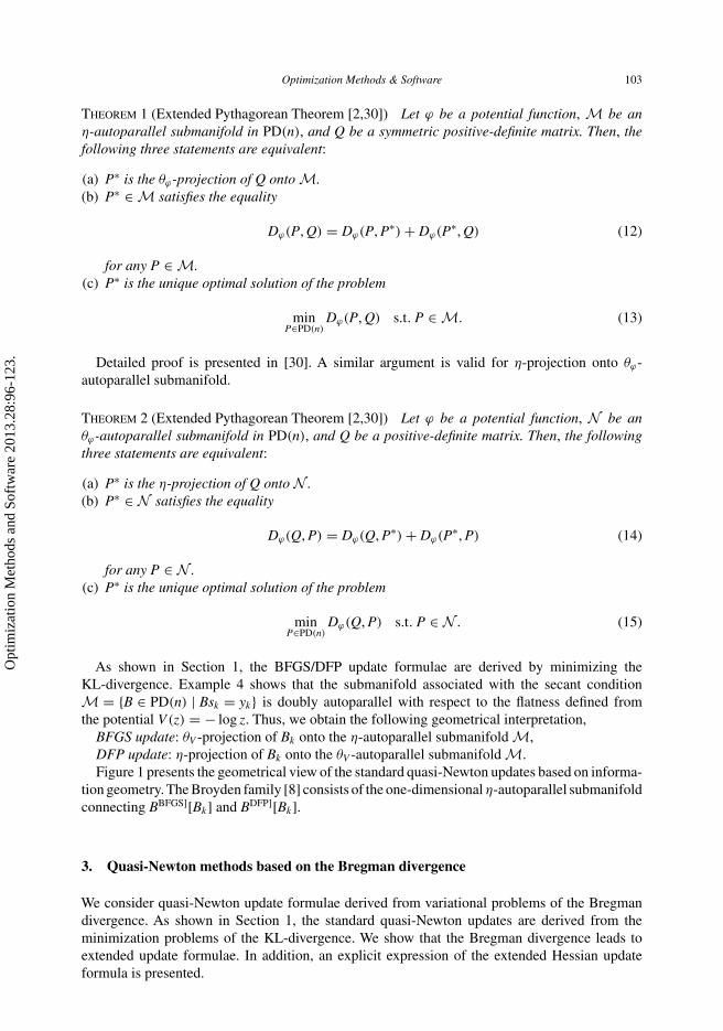
As shown in Section 1, the BFGS/DFP update formulae are derived by minimizing theKL-divergence. Example 4 shows that the submanifold associated with the secant conditionM = {B ∈ PD(n) | Bsk = yk} is doubly autoparallel with respect to the flatness defined fromthe potential V(z) = − log z. Thus, we obtain the following geometrical interpretation,

BFGS update: θV -projection of Bk onto the η-autoparallel submanifold M,DFP update: η-projection of Bk onto the θV -autoparallel submanifold M.Figure 1 presents the geometrical view of the standard quasi-Newton updates based on informa-

tion geometry. The Broyden family [8] consists of the one-dimensional η-autoparallel submanifoldconnecting BBFGS][Bk] and BDFP][Bk].

3. Quasi-Newton methods based on the Bregman divergence

We consider quasi-Newton update formulae derived from variational problems of the Bregmandivergence. As shown in Section 1, the standard quasi-Newton updates are derived from theminimization problems of the KL-divergence. We show that the Bregman divergence leads toextended update formulae. In addition, an explicit expression of the extended Hessian updateformula is presented.

Opt

imiz

atio

n M

etho

ds a

nd S

oftw

are

2013

.28:

96-1

23.


Bk

BBFGS[Bk]BDFP [Bk]

θV -projection(V (z) = − log z)

η-projection

M = {B ∈ PD(n) | Bs = y}Secant condition: doubly-autoparallel

M

Figure 1. Geometrical interpretation of quasi-Newton updates. For the potential V(z) = − log z, the submanifold Mdefined by the secant condition is doubly autoparallel with respect to the η- and θV -coordinate systems. The BFGS formulaBBFGS[Bk] is given as the θV -projection of Bk onto the η-autoparallel submanifold M, and the DFP update BDFP[Bk] isgiven as the η-projection of Bk onto the θV -autoparallel submanifold M.

We consider the minimization problem of the Bregman divergence instead of the KL-divergence. An extended BFGS update formula is defined as the optimal solution of

minB∈PD(n)

Dϕ(B, Bk) s.t. Bsk = yk . (16)

Suppose that the optimal solution Bk+1 exists. Then, Bk+1 is the unique θϕ-projection of Bk ontothe submanifold corresponding to the secant condition. On the other hand, as an extension of theDFP update, we consider the problem,

minB∈PD(n)

Dϕ(B−1, B−1k ) s.t. Bsk = yk (17)

instead of the minimization of KL(Bk , B) = KL(B−1, B−1k ). In a similar way, we can derive an

extended quasi-Newton update formulae for the approximate inverse Hessian matrix Hk = B−1k .

In the following, we focus on the extension of the BFGS method (16), since the same argumentis valid for the extension of the DFP method (17). A formal expression of the optimal solution ispresented in the following theorem.

Theorem 3 Suppose that there exists an optimal solution (16). Then the optimal solution Bk+1

is unique and satisfies

Bk+1 = ∇ϕ∗(∇ϕ(Bk) + skλ� + λs�

k ), Bk+1sk = yk ,

where λ ∈ Rn is a column vector and ϕ∗ is the Fenchel conjugate function of ϕ.

Proof Since (16) is a convex problem and the objective function Dϕ(B, Bk) is strictly convexin B, we see that the optimal solution is unique if it exists. Suppose that Bk+1 is the optimal solutionof (16), then Bk+1 satisfies the optimality condition. According to Güler et al. [22], the normalvector of the affine subspace M = {B ∈ PD(n) | Bsk = yk} is characterized by the form of

skλ� + λs�

k ∈ Sym(n), λ ∈ Rn.

In fact for B1, B2 ∈ M we have

〈skλ� + λs�

k , B1 − B2〉 = λ�B1sk + s�k B1λ − λ�B2sk − s�

k B2λ

= λ�yk + y�k λ − λ�yk − y�

k λ

= 0,

Opt

imiz

atio

n M

etho

ds a

nd S

oftw

are

2013

.28:

96-1

23.


and thus skλ� + λs�

k is a normal vector of M. Güler et al. [22] have shown that the normalvector is restricted to the expression above. Hence, for the optimal solution Bk+1 there existsλ ∈ R

n such that ∇Dϕ(B, Bk)|B=Bk+1 = skλ� + λs�

k and Bk+1sk = yk hold. The first equality isrepresented as ∇ϕ(Bk+1) − ∇ϕ(Bk) = skλ

� + λs�k . The existence of Bk+1 assures that Bk+1 =

∇ϕ∗(∇ϕ(Bk) + skλ� + λs�

k ), where ϕ∗ is the Fenchel conjugate of ϕ defined in (11). �

For the general Bregman divergence Dϕ , we do not have the explicit expression of the Hessianupdate formula. As a special case, we consider the minimization problem of the V -Bregmandivergence,

V -BFGS: minB∈PD(n)

DV (B, Bk) s.t. Bsk = yk . (18)

The update formula obtained by (18) is referred to as the V -BFGS update formula. The theorembelow shows the explicit expression of the V -BFGS update formula.

Theorem 4 (V -BFGS update formula) Suppose the function V is a potential function definedin Definition 2. Let Bk ∈ PD(n), and suppose s�

k yk > 0. Then, the problem (18) has the uniqueoptimal solution Bk+1 ∈ PD(n) such that

Bk+1 = ν(det Bk+1)

ν(det Bk)BBFGS[Bk; sk , yk] +

(1 − ν(det Bk+1)

ν(det Bk)

)yky�

k

s�k yk

. (19)

Though the theorem is proved in [24], the proof is also found in Appendix 1 of the present paperas a supplementary. In the same way, we can obtain the explicit formula of the V -DFP updateformula, which is the minimizer of DV (B−1, B−1

k ) subject to Bsk = yk . The potential V(z) =− log z leads to ν(z) = 1, and then, the V -BFGS update formula is reduced to the standard BFGSformula. We can define an extended Broyden family such that the one-dimensional η-autoparallelsubmanifold connects the V1-BFGS and the V2-DFP update formulae.

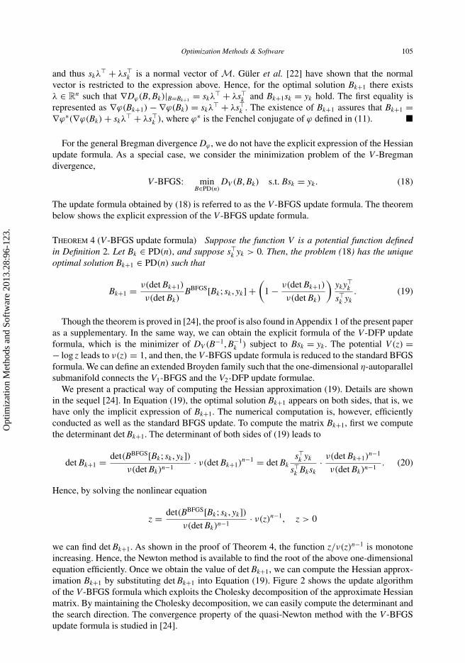
We present a practical way of computing the Hessian approximation (19). Details are shownin the sequel [24]. In Equation (19), the optimal solution Bk+1 appears on both sides, that is, wehave only the implicit expression of Bk+1. The numerical computation is, however, efficientlyconducted as well as the standard BFGS update. To compute the matrix Bk+1, first we computethe determinant det Bk+1. The determinant of both sides of (19) leads to

det Bk+1 = det(BBFGS[Bk; sk , yk])ν(det Bk)n−1

· ν(det Bk+1)n−1 = det Bk

s�k yk

s�k Bksk

· ν(det Bk+1)n−1

ν(det Bk)n−1. (20)

Hence, by solving the nonlinear equation

z = det(BBFGS[Bk; sk , yk])ν(det Bk)n−1

· ν(z)n−1, z > 0

we can find det Bk+1. As shown in the proof of Theorem 4, the function z/ν(z)n−1 is monotoneincreasing. Hence, the Newton method is available to find the root of the above one-dimensionalequation efficiently. Once we obtain the value of det Bk+1, we can compute the Hessian approx-imation Bk+1 by substituting det Bk+1 into Equation (19). Figure 2 shows the update algorithmof the V -BFGS formula which exploits the Cholesky decomposition of the approximate Hessianmatrix. By maintaining the Cholesky decomposition, we can easily compute the determinant andthe search direction. The convergence property of the quasi-Newton method with the V -BFGSupdate formula is studied in [24].

Opt

imiz

atio

n M

etho

ds a

nd S

oftw

are

2013

.28:

96-1

23.


Figure 2. Pseudo-code of the V -BFGS method. The Cholesky decomposition with rank-one update [18] is useful in thealgorithm.

The update formula (19) is included in the class of the self-scaling quasi-Newton updateformulae defined as

Bk+1 = τkBBFGS[Bk; sk , yk] + (1 − τk)yky�

k

s�k yk

, (21)

where τk is a positive real number. Various choices for τk have been proposed; see [34,37].A popular choice is τk = s�

k yk/s�k Bksk . In the V -BFGS update formula, the coefficient τk is

determined from the function ν.

Example 5 We show the V -BFGS formula derived from the power potential. Let V(z) be thepower potential V(z) = (1 − zγ )/γ with γ < 1/n. As shown in Example 2, we have ν(z) = zγ .Due to the equality

det(BBFGS[Bk; sk , yk]) = det(Bk)s�

k yk

s�k Bksk

and Equation (20), we have

ν(det Bk+1)

ν(det Bk)=

(s�

k yk

s�k Bksk

)ρ

, ρ = γ

1 − (n − 1)γ.

Opt

imiz

atio

n M

etho

ds a

nd S

oftw

are

2013

.28:

96-1

23.


Then, the V -BFGS update formula is given as

Bk+1 =(

s�k yk

s�k Bksk

)ρ

BBFGS[Bk; sk , yk] +(

1 −(

s�k yk

s�k Bksk

)ρ)yky�

k

s�k yk

. (22)

For γ such that γ < 1/n, we have −1/(n − 1) < ρ < 1. In the standard self-scaling updateformula (21), the above matrix Bk+1 with ρ = 1 (γ = 1/n) is used, while it is not derived fromthe strictly convex potential function. For the (pseudo-) Bregman divergence defined from thepower potential with γ = 1/n, it is easy to see the equality DV (P, Q) = 0 holds if and only ifthere exists c > 0 such that Q = cP. If the secant condition M = {B ∈ PD(n) | Bsk = yk} is nota cone, DV (B, Bk) is strictly convex on M. Hence, the update formula defined by (18) is uniquelydetermined as the form of (22) with ρ = 1.

4. Invariance of update formulae under group action

In this section we study the invariance of the V -BFGS update formula (19) under affine trans-formations of the optimization variable. We consider linear transformations instead of affinetransformations for the sake of simplicity. For the minimization problem of the function f (x), letus consider the variable change of x. For a non-degenerate matrix T ∈ GL(n), the variable changefrom x to x is defined by

x = T−1x. (23)

Then, the function f (x) is transformed to f (x) such that

f (x) = f (T−1x).

Some calculation yields

∇ f (x) = (T�)−1∇f (T−1x), ∇2 f (x) = (T�)−1(∇2f (T−1x))T−1.

Our concern is how the point sequence {xk}∞k=1 generated by the V -BFGS method is transformedby the variable change (23).

We consider the Hessian approximation matrix under the variable change, x = Tx. Let Bk ∈PD(n) be the Hessian approximation computed at the kth step of the V -BFGS update for theminimization of f (x). We now define

xk = Txk , Bk = (T�)−1BkT−1.

Let Bk+1 be the Hessian approximation matrix updated from Bk for the function f (x), where theV -BFGS method is used. We consider the relation between Bk+1 and Bk+1. Let αk be a step lengthat the point xk , that is,

xk+1 = xk − αkB−1k ∇f (xk).

On the other hand, the updated point xk+1 for the function f (x) is given as

xk+1 = xk − αkB−1k ∇ f (xk),

where αk is a step length determined by a line search for f . Note that, for any α ∈ R, the equality

f (xk − αB−1k ∇ f (xk)) = f (T(xk − αB−1

k ∇f (T−1xk))) = f (xk − αB−1k ∇f (xk)) (24)

Opt

imiz

atio

n M

etho

ds a

nd S

oftw

are

2013

.28:

96-1

23.


holds. Hence, f (xk − αB−1k ∇ f (xk)) and f (xk − αB−1

k ∇f (xk)) are the same as the function of α.The derivative of (24) with respect to α leads to

∇ f (xk − αB−1k ∇ f (xk))

�B−1k ∇ f (xk) = ∇f (xk − αB−1

k ∇f (xk))�B−1

k ∇f (xk)

for all α ∈ R, and then, we obtain

∇ f (xk)�B−1

k ∇ f (xk) = ∇f (xk)�B−1

k ∇f (xk)

by substituting α = 0. In most inaccurate line search procedures, the quantity ∇f (xk)�B−1

k ∇f (xk)

is used for efficient computation of minα≥0 f (xk − αB−1k ∇f (xk)) [27, Section 8.5]. As a result, if

the same line search method, e.g. the Wolfe condition with the same parameters, is used to bothf (x) and f (x), the step length αk is identical to αk . Then, under the condition αk = αk , the equalityxk+1 = Txk+1 holds. Let sk and yk be

sk = xk+1 − xk , yk = ∇ f (xk+1) − ∇ f (xk),

then, we obtain the equalities,

sk = Tsk , yk = (T�)−1yk .

We consider the condition of T such that the equality

T�Bk+1T = Bk+1, (25)

holds, when xk = Txk and Bk = (T�)−1BkT−1 are satisfied. If (25) holds, the equality xk+1 =Txk+1 recursively holds. This implies that the point sequence obtained by the V -BFGS method isinvariant under the linear transformation (23). In the optimization of f (x) by the V -BFGS method,the matrix Bk is updated to Bk+1 such that

Bk+1 = ν(det Bk+1)


(1 − ν(det Bk+1)

ν(det Bk)

)yk y�

k

s�k yk

.

The above equality leads to

T�Bk+1T = ν(det Bk+1)


(1 − ν(det Bk+1)

ν(det Bk)

)yky�

k

s�k yk

. (26)

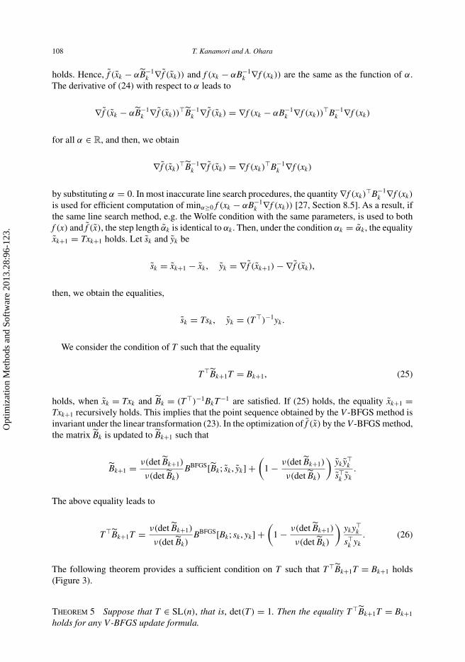
The following theorem provides a sufficient condition on T such that T�Bk+1T = Bk+1 holds(Figure 3).

Theorem 5 Suppose that T ∈ SL(n), that is, det(T) = 1. Then the equality T�Bk+1T = Bk+1

holds for any V-BFGS update formula.

Opt

imiz

atio

n M

etho

ds a

nd S

oftw

are

2013

.28:

96-1

23.


x0

−B−10 ∇f (x0)

xkx0 = Tx0

−B−10 ∇f (x0)

xk

T

T−1

f (x)

f (x)

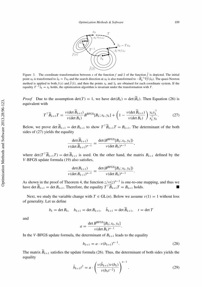
Figure 3. The coordinate transformation between x of the function f and x of the function f is depicted. The initialpoint x0 is transformed to x0 = Tx0 and the search direction at x0 is also transformed to −B−1

0 ∇ f (x0). The quasi-Newtonmethod is applied to both f (x) and f (x), and then the points xk and xk are obtained for each coordinate system. If theequality T−1xk = xk holds, the optimization algorithm is invariant under the transformation with T .

Proof Due to the assumption det(T) = 1, we have det(Bk) = det(Bk). Then Equation (26) isequivalent with

T�Bk+1T = ν(det Bk+1)


(1 − ν(det Bk+1)

ν(det Bk)

)yky�

k

s�k yk

. (27)

Below, we prove det Bk+1 = det Bk+1 to show T�Bk+1T = Bk+1. The determinant of the bothsides of (27) yields the equality

det(Bk+1)

ν(det Bk+1)n−1= det(BBFGS[Bk; sk , yk])

ν(det Bk)n−1,

where det(T�Bk+1T) = det Bk+1 is used. On the other hand, the matrix Bk+1 defined by theV -BFGS update formula (19) also satisfies,

det(Bk+1)

ν(det Bk+1)n−1= det(BBFGS[Bk; sk , yk])

ν(det Bk)n−1.

As shown in the proof of Theorem 4, the function z/ν(z)n−1 is one-to-one mapping, and thus wehave det Bk+1 = det Bk+1. Therefore, the equality T�Bk+1T = Bk+1 holds. �

Next, we study the variable change with T ∈ GL(n). Below we assume ν(1) = 1 without lossof generality. Let us define

bk = det Bk , bk+1 = det Bk+1, bk+1 = det Bk+1, t = det T

and

a = det BBFGS[Bk; sk , yk]ν(det Bk)n−1

.

In the V -BFGS update formula, the determinant of Bk+1 leads to the equality

bk+1 = a · ν(bk+1)n−1. (28)

The matrix Bk+1 satisfies the update formula (26). Thus, the determinant of both sides yields theequality

bk+1t2 = a ·(

ν(bk+1)ν(bk)

ν(bkt−2)

)n−1

. (29)

Opt

imiz

atio

n M

etho

ds a

nd S

oftw

are

2013

.28:

96-1

23.


If T�Bk+1T = Bk+1 holds, Equation (29) is represented as

bk+1 = a ·(

ν(bk+1t−2)ν(bk)

ν(bkt−2)

)n−1

. (30)

We consider the function ν which satisfies (28) and (30) simultaneously. For a positive numbera > 0, let ba be the unique solution of the equation of b,

b = a · ν(b)n−1, b > 0,

and Eν = {ba ∈ R | a > 0} be the set of all possible solutions of the above equation. Note that1 ∈ Eν holds for any ν, since 1 = 1 · ν(1)n−1 holds.

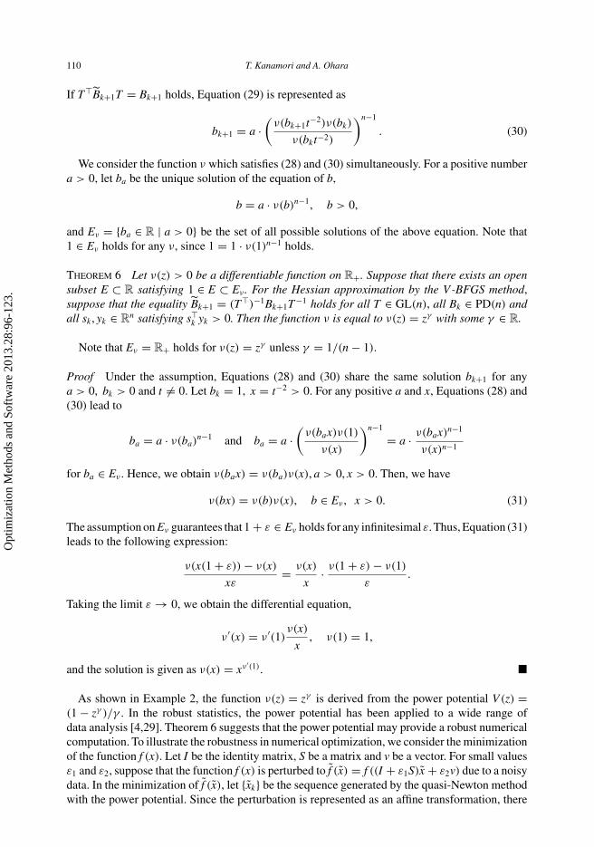
Theorem 6 Let ν(z) > 0 be a differentiable function on R+. Suppose that there exists an opensubset E ⊂ R satisfying 1 ∈ E ⊂ Eν . For the Hessian approximation by the V-BFGS method,suppose that the equality Bk+1 = (T�)−1Bk+1T−1 holds for all T ∈ GL(n), all Bk ∈ PD(n) andall sk , yk ∈ R

n satisfying s�k yk > 0. Then the function ν is equal to ν(z) = zγ with some γ ∈ R.

Note that Eν = R+ holds for ν(z) = zγ unless γ = 1/(n − 1).

Proof Under the assumption, Equations (28) and (30) share the same solution bk+1 for anya > 0, bk > 0 and t �= 0. Let bk = 1, x = t−2 > 0. For any positive a and x, Equations (28) and(30) lead to

ba = a · ν(ba)n−1 and ba = a ·

(ν(bax)ν(1)

ν(x)

)n−1

= a · ν(bax)n−1

ν(x)n−1

for ba ∈ Eν . Hence, we obtain ν(bax) = ν(ba)ν(x), a > 0, x > 0. Then, we have

ν(bx) = ν(b)ν(x), b ∈ Eν , x > 0. (31)

The assumption on Eν guarantees that 1 + ε ∈ Eν holds for any infinitesimal ε. Thus, Equation (31)leads to the following expression:

ν(x(1 + ε)) − ν(x)

xε= ν(x)

x· ν(1 + ε) − ν(1)

ε.

Taking the limit ε → 0, we obtain the differential equation,

ν ′(x) = ν ′(1)ν(x)

x, ν(1) = 1,

and the solution is given as ν(x) = xν ′(1). �

As shown in Example 2, the function ν(z) = zγ is derived from the power potential V(z) =(1 − zγ )/γ . In the robust statistics, the power potential has been applied to a wide range ofdata analysis [4,29]. Theorem 6 suggests that the power potential may provide a robust numericalcomputation. To illustrate the robustness in numerical optimization, we consider the minimizationof the function f (x). Let I be the identity matrix, S be a matrix and v be a vector. For small valuesε1 and ε2, suppose that the function f (x) is perturbed to f (x) = f ((I + ε1S)x + ε2v) due to a noisydata. In the minimization of f (x), let {xk} be the sequence generated by the quasi-Newton methodwith the power potential. Since the perturbation is represented as an affine transformation, there

Opt

imiz

atio

n M

etho

ds a

nd S

oftw

are

2013

.28:

96-1

23.


exists the sequence {xk} generated by the same quasi-Newton method for the function f (x) suchthat the equality

xk = (I + ε1S)xk + ε2v

holds for all k. The sequence {xk} is regarded as the ideal one in the noiseless situation, and theinequality

‖xk − xk‖ ≤ ε1‖Sxk‖ + ε2‖v‖holds for all k. This result guarantees that the optimization algorithm is robust against the pertur-bation of the objective function. For the V -BFGS method with the potential other than the powerpotential, we will need more involved analysis to evaluate the difference between xk and xk unlessthe equality det (I + ε1S) = 1 holds.

Remark 1 Ohara and Eguchi [36] have studied the differential geometrical structure on PD(n)

induced by the V -Bregman divergence. They pointed out that the geometrical structure is invariantunder the SL(n) group action. Furthermore, they have showed that, for the power potential V(z) =(1 − zγ )/γ , the θV - (η-) projection onto η- (θV -) autoparallel submanifold is invariant under theGL(n) group action. It turns out that only the orthogonality is kept unchanged under the groupaction. The other geometrical features, such as the angle between two tangent vectors, are notpreserved in general. Theorem 6 indicates that the invariance of the geometrical structure onPD(n) is inherited to the invariance of point sequences of quasi-Newton methods under affinetransformations.

In summary, we obtain the following results. Suppose that x0 = Tx0 + v, B0 = (T�)−1B0T−1

holds for a matrix T and a vector v. Let {xk} and {xk} be point sequences generated by the V -BFGSmethod using the same line search for the functions f (x) and f (x), respectively. Then, for any T ∈SL(n), the equality xk = Txk + v holds for all k ≥ 1. Moreover, the equality xk = Txk + v, k ≥ 1holds for any T ∈ GL(n) if and only if the function V(z) is the power potential.

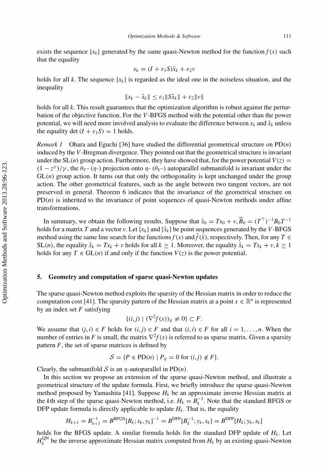
5. Geometry and computation of sparse quasi-Newton updates

The sparse quasi-Newton method exploits the sparsity of the Hessian matrix in order to reduce thecomputation cost [41]. The sparsity pattern of the Hessian matrix at a point x ∈ R

n is representedby an index set F satisfying

{(i, j) | (∇2f (x))ij �= 0} ⊂ F.

We assume that (j, i) ∈ F holds for (i, j) ∈ F and that (i, i) ∈ F for all i = 1, . . . , n. When thenumber of entries in F is small, the matrix ∇2f (x) is referred to as sparse matrix. Given a sparsitypattern F, the set of sparse matrices is defined by

S = {P ∈ PD(n) | Pij = 0 for (i, j) �∈ F}.Clearly, the submanifold S is an η-autoparallel in PD(n).

In this section we propose an extension of the sparse quasi-Newton method, and illustrate ageometrical structure of the update formula. First, we briefly introduce the sparse quasi-Newtonmethod proposed by Yamashita [41]. Suppose Hk be an approximate inverse Hessian matrix atthe kth step of the sparse quasi-Newton method, i.e. Hk = B−1

k . Note that the standard BFGS orDFP update formula is directly applicable to update Hk . That is, the equality

Hk+1 = B−1k+1 = BBFGS[Bk; sk , yk]−1 = BDFP[B−1

k ; yk , sk] = BDFP[Hk; yk , sk]holds for the BFGS update. A similar formula holds for the standard DFP update of Hk . LetHQN

k be the inverse approximate Hessian matrix computed from Hk by an existing quasi-Newton

Opt

imiz

atio

n M

etho

ds a

nd S

oftw

are

2013

.28:

96-1

23.


method such as the BFGS or DFP method. In the sparse quasi-Newton method, we need only thepartial matrix (HQN

k )ij, (i, j) ∈ F, and hence efficient computation will be possible, even if thesize of the matrix is large. Then, the matrix Hk+1 is defined as the optimal solution of

minH∈PD(n)

KL(H−1, (HQNk )−1) s.t. H−1 ∈ S. (32)

The constraint H−1 ∈ S is imposed, since Hk+1 is an approximate matrix of the inverse Hessian.The optimality condition of the above problem is given as

(H−1)ij = 0, (i, j) �∈ F,

Hij = (HQNk )ij, (i, j) ∈ F.

Indeed, the Lagrange function of (32) for the variable B = H−1 is equal to

tr(BHQNk ) − log det(BHQN

k ) − n −∑

(i,j)�∈F

μijBij,

and the derivative with respect to Bij, (i, j) ∈ F leads to the equality (HQNk )ij − (B−1)ij = 0. The

updated matrix Hk+1 is uniquely determined by the above optimality condition. The calculation ofH−1

k+1 from (HQNk )−1 is regarded as the θV -projection onto S with respect to the KL-divergence. The

sparse clique-factorization technique [17,21] is available for the practical computation of Hk+1.The matrix Hk+1 is used as an approximate inverse Hessian matrix at xk+1. Note that generallyHk+1 does not satisfy the secant condition H−1

k+1xk = yk . See [41] for details.We extend the sparse quasi-Newton method by using the Bregman divergence instead of the KL-

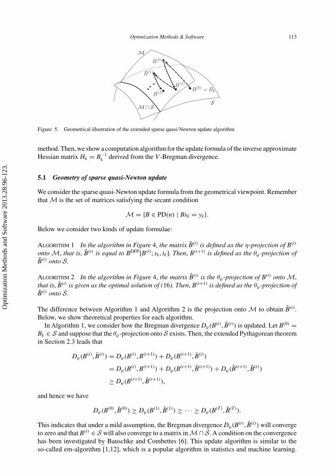
divergence. Figure 4 shows an extended sparse quasi-Newton method for the approximate Hessianmatrix Bk . Figure 5 illustrates the geometrical interpretation of the extended sparse quasi-Newtonupdates. In Figures 4 and 5, the updated sequence of the approximate Hessian Bk is illustrated,while the computation is conducted in the inverse side, Hk = B−1

k .In the algorithm of Figure 4, we have some choices: (i) the Bregman divergence in Step 1,

(ii) projection in Step 2 and (iii) the number of T . In the sparse quasi-Newton updates presentedby Yamashita [41], the number of iteration is set to T = 1; in Step 1, the standard BFGS/DFPmethod for the approximate inverse Hessian is used; in Step 2 the θV -projection defined from theKL-divergence is computed. Moreover, the superlinear convergence has been proved, see [41]for details. In the following, we present a geometrical interpretation of the sparse quasi-Newton

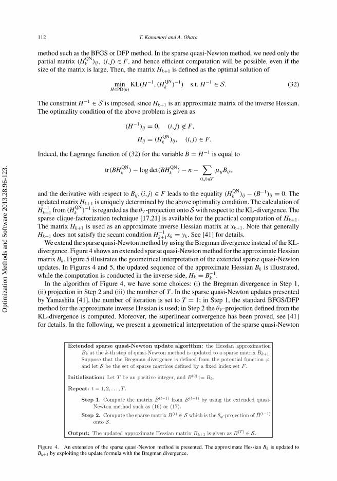
Extended sparse quasi-Newton update algorithm: the Hessian approximationBk at the k-th step of quasi-Newton method is updated to a sparse matrix Bk+1.Suppose that the Bregman divergence is defined from the potential function ϕ,and let S be the set of sparse matrices defined by a fixed index set F .

Initialization: Let T be an positive integer, and B(0) := Bk.

Repeat: t = 1, 2, . . . , T .

Step 1. Compute the matrix B(t−1) from B(t−1) by using the extended quasi-Newton method such as (16) or (17).

Step 2. Compute the sparse matrix B(t) ∈ S which is the θϕ-projection of B(t−1)

onto S.

Output: The updated approximate Hessian matrix Bk+1 is given as B(T ) ∈ S.

Figure 4. An extension of the sparse quasi-Newton method is presented. The approximate Hessian Bk is updated toBk+1 by exploiting the update formula with the Bregman divergence.

Opt

imiz

atio

n M

etho

ds a

nd S

oftw

are

2013

.28:

96-1

23.


B(0) = BkB(1)

B(2)

B(0)

B(1)

M

SM ∩ S

Figure 5. Geometrical illustration of the extended sparse quasi-Newton update algorithm.

method. Then, we show a computation algorithm for the update formula of the inverse approximateHessian matrix Hk = B−1

k derived from the V -Bregman divergence.

5.1 Geometry of sparse quasi-Newton update

We consider the sparse quasi-Newton update formula from the geometrical viewpoint. Rememberthat M is the set of matrices satisfying the secant condition

M = {B ∈ PD(n) | Bsk = yk}.Below we consider two kinds of update formulae:

Algorithm 1 In the algorithm in Figure 4, the matrix B(t) is defined as the η-projection of B(t)

onto M, that is, B(t) is equal to BDFP[B(t); sk , tk]. Then, B(t+1) is defined as the θϕ-projection ofB(t) onto S.

Algorithm 2 In the algorithm in Figure 4, the matrix B(t) is the θϕ-projection of B(t) onto M,that is, B(t) is given as the optimal solution of (16). Then, B(t+1) is defined as the θϕ-projection ofB(t) onto S.

The difference between Algorithm 1 and Algorithm 2 is the projection onto M to obtain B(t).Below, we show theoretical properties for each algorithm.

In Algorithm 1, we consider how the Bregman divergence Dϕ(B(t), B(t)) is updated. Let B(0) =Bk ∈ S and suppose that the θϕ-projection onto S exists. Then, the extended Pythagorean theoremin Section 2.3 leads that

Dϕ(B(t), B(t)) = Dϕ(B(t), B(t+1)) + Dϕ(B(t+1), B(t))

= Dϕ(B(t), B(t+1)) + Dϕ(B(t+1), B(t+1)) + Dϕ(B(t+1), B(t))

≥ Dϕ(B(t+1), B(t+1)),

and hence we have

Dϕ(B(0), B(0)) ≥ Dϕ(B(1), B(1)) ≥ · · · ≥ Dϕ(B(T), B(T)).

This indicates that under a mild assumption, the Bregman divergence Dϕ(B(t), B(t)) will convergeto zero and that B(t) ∈ S will also converge to a matrix in M ∩ S. A condition on the convergencehas been investigated by Bauschke and Combettes [6]. This update algorithm is similar to theso-called em-algorithm [1,12], which is a popular algorithm in statistics and machine learning.

Opt

imiz

atio

n M

etho

ds a

nd S

oftw

are

2013

.28:

96-1

23.


In the em-algorithm, the η-projection and the θV -projection defined from the KL-divergenceis repeated in the probability space. Then, the maximum likelihood estimator under a partialobservation is computed. In the context of statistical estimation, usually the em-algorithm isconducted, whenM ∩ S = ∅holds. Under some assumption withM ∩ S = ∅, the point sequence(B(t), B(t)) ∈ S × M converges to the pair (B∗, B∗) ∈ S × M, which is the optimal solution of

min(B,B)∈S×M

Dϕ(B, B),

see [28] for details. Up to our knowledge, showing a simple characterization about the convergencepoint (B∗, B∗) under the condition M ∩ S �= ∅ is an open problem.

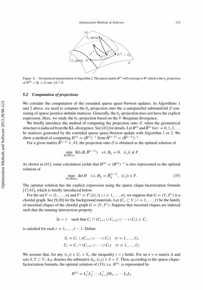
Next, we investigate Algorithm 2. Likewise, we suppose Bk = B(0) ∈ S. Note that M ∩ S isη-autoparallel. Let B� be the θϕ-projection of Bk = B(0) onto the intersection M ∩ S. Then theextended Pythagorean theorem leads to

Dϕ(B�, B(t)) = Dϕ(B�, B(t)) + Dϕ(B(t), B(t))

= Dϕ(B�, B(t+1)) + Dϕ(B(t+1), B(t)) + Dϕ(B(t), B(t))

≥ Dϕ(B�, B(t+1)),

and hence we have

Dϕ(B�, B(0)) ≥ Dϕ(B�, B(1)) ≥ · · · ≥ Dϕ(B�, B(T)).

Suppose that B(T) converges to B(∞) ∈ M ∩ S when T tends to infinity. Then, the equalityB(∞) = B� holds as shown below. From the definition of B� and the extended Pythagorean theorem,we have

Dϕ(B(∞), B(T)) = Dϕ(B(∞), B�) + Dϕ(B�, B(T)).

Due to the continuity of the Bregman divergence, for T → ∞ we have

0 = Dϕ(B(∞), B(∞)) = Dϕ(B(∞), B�) + Dϕ(B�, B(∞)),

and hence B(∞) = B� holds. As a result, we have limT→∞ B(T) = B�. Figure 6 shows the geomet-rical illustration of Algorithm 2. Applying Theorem 8.1 of Bauschke and Borwein [5], we seethat the convergence of B(T) to the point B� is guaranteed for the Bregman divergence associatedwith power potential with γ ≤ 0. The iterative update procedure is closely related to the boost-ing algorithm [16,30], which is used to solve statistical classification problems. In the boostingalgorithm, typically there are many η-autoparallel submanifolds, and the Bregman projection ontoeach submanifold is repeated to achieve the intersection of these submanifolds.

As argued above, it is not guaranteed that B(t) in Algorithm 1 converges to B�, which is theθϕ-projection of Bk = B(0) onto M ∩ S. On the other hand, the sequence B(t) in Algorithm 2converges to B� under mild assumption. From the viewpoint of the least-change principle, thesparse quasi-Newton method with Algorithm 2 will be preferable. Fletcher [15] has proposedthe sparse update formula using B�. As shown in [39], B� sometimes becomes unstable due to thesimultaneous requirement of the sparsity and the secant condition. Hence, the extended sparsequasi-Newton method with large T will not be advantageous for computational efficiency andnumerical stability.

Opt

imiz

atio

n M

etho

ds a

nd S

oftw

are

2013

.28:

96-1

23.


B(0) = BkB(1)

B(2)

M

Sθϕ-proj. B

θϕ-proj.

Figure 6. Geometrical interpretation ofAlgorithm 2. The sparse matrix B(t) will converge to B� which is the θϕ projectionof B(0) = Bk ∈ S onto M ∩ S.

5.2 Computation of projections

We consider the computation of the extended sparse quasi-Newton updates. In Algorithms 1and 2 above, we need to compute the θϕ-projection onto the η-autoparallel submanifold S con-sisting of sparse positive-definite matrices. Generally, the θϕ-projection does not have the explicitexpression. Here, we study the θV -projection based on the V -Bregman divergence.

We briefly introduce the method of computing the projection onto S, when the geometricalstructure is induced from the KL-divergence. See [41] for details. Let B(t) and B(t) for t = 0, 1, 2, . . .be matrices generated by the extended sparse quasi-Newton update with Algorithm 1 or 2. Weshow a method of computing H(t) = (B(t))−1 from H(t−1) = (B(t−1))−1.

For a given matrix B(t−1) ∈ M, the projection onto S is obtained as the optimal solution of

minB∈PD(n)

KL(B, B(t−1)) s.t. Bij = 0, (i, j) �∈ F.

As shown in [41], some calculation yields that H(t) = (B(t))−1 is also represented as the optimalsolution of

maxH∈PD(n)

det H s.t. Hij = H(t−1)ij , (i, j) ∈ F. (33)

The optimal solution has the explicit expression using the sparse clique-factorization formula[17,41], which is briefly introduced below.

For the set V = {1, . . . , n} and F◦ = F\{(i, i) | i = 1, . . . , n}, we suppose that G = (V , F◦) is achordal graph. See [9,20] for the background materials. Let {Cr ⊂ V | r = 1, . . . , �} be the familyof maximal cliques of the chordal graph G = (V , F◦). Suppose that maximal cliques are indexedsuch that the running intersection property

∃s > r such that Cr ∩ (Cr+1 ∪ Cr+2 ∪ · · · ∪ C�) ⊂ Cs

is satisfied for each r = 1, . . . , � − 1. Define

Sr = Cr \ (Cr+1 ∪ · · · ∪ C�) (r = 1, . . . , �),

Ur = Cr ∩ (Cr+1 ∪ · · · ∪ C�) (r = 1, . . . , �).

We assume that, for any (i, j) ∈ Ur × Sr , the inequality i > j holds. For an n × n matrix A andsets S, T ⊂ V , AST denotes the submatrix Aij, (i, j) ∈ S × T . Then, according to the sparse clique-factorization formula, the optimal solution of (33), i.e. H(t), is represented by

H(t) = L�1 L�

2 · · · L��−1DL�−1 · · · L2L1

Opt

imiz

atio

n M

etho

ds a

nd S

oftw

are

2013

.28:

96-1

23.


in which Lr (r = 1, . . . , � − 1) are lower triangular matrices,

(Lr)ij =

⎧⎪⎨⎪⎩1, i = j,

(H(t−1)Ur Ur

)−1H(t−1)Ur Sr

, (i, j) ∈ Ur × Sr ,

0 otherwise

(34)

and D is a positive-definite block-diagonal matrix consisting of � diagonal blocks,

D =

⎛⎜⎜⎜⎝DS1S1

DS2S2

. . .DS�S�

⎞⎟⎟⎟⎠ , (35)

DSr Sr ={

H(t−1)Sr Sr

− H(t−1)Sr Ur

(H(t−1)Ur Ur

)−1H(t−1)Ur Sr

, r = 1, . . . , � − 1,

H(t−1)S�S�

, r = �.(36)

All elements of Lr (r = 1, . . . , � − 1) and D are explicitly computed only from the submatri-ces H(t−1)

Cr Cr, (r = 1, . . . , �), and these submatrices are identical to H(t)

Cr Cr, (r = 1, . . . , �) due to the

constraint in (33).Next we consider a characterization of the projection with respect to the V -Bregman divergence.

Theorem 7 Let B(t−1) ∈ M. Then there exists the θV -projection of B(t−1) onto S, and theprojection B(t) is the unique optimal solution of the problem,

minB∈PD(n)

det(B) s.t. (θV (B))ij = (θV (B(t−1)))ij, (i, j) ∈ F. (37)

Proof Remember that θV (P) is defined as θV (P) = −ν(det P)P−1 which is a negative-definitematrix. It is easy to see that the mapping −θV (P) is bijection on PD(n). As shown in [11,21], theproblem

maxB∈PD(n)

det(−θV (B)), (θV (B))ij = (θV (B(t−1)))ij for all (i, j) ∈ F (38)

has the unique optimal solution B∗, and the optimal solution satisfies (−θV (B∗))−1 ∈ S, that is,B∗

ij = 0 for (i, j) �∈ F. In terms of the objective function in (38), we see that

det(−θV (B)) = det(ν(det B)B−1) = ν(det B)n

det B.

The function ν(z)n/z is strictly monotone decreasing for z > 0. Indeed,

d

dzlog

ν(z)n

z= n

z

(β(z) − 1

n

)< 0

holds. Thus, the optimal solution of (38) is identical to that of (37). For any B ∈ S, we have

DV (B, B(t−1)) − DV (B, B∗) − DV (B∗, B(t−1)) =∑

i,j

(θV (B(t−1)) − θV (B∗))ij(B∗ − B)ij

=∑

(i,j)�∈F

(θV (B(t−1)) − θV (B∗))ij(B∗ − B)ij

= 0.

Opt

imiz

atio

n M

etho

ds a

nd S

oftw

are

2013

.28:

96-1

23.


The second and third equalities follow (θV (B(t−1)) − θV (B∗))ij = 0 for (i, j) ∈ F and(B∗ − B)ij = 0 for (i, j) �∈ F, respectively. Therefore, Theorem 1 guarantees that B∗ is identi-cal to the θV -projection of B(t−1) onto S. As a result, we have B(t) = B∗ which is the optimalsolution of (37). �

For the optimal solution B(t) of (37), the inverse H(t) = (B(t))−1 is expressed in the form of thesparse clique-factorization, if the graph G = (V , F◦) is chordal. Indeed, from (38) we see that−θV (B(t)) = ν((det H(t))−1)H(t) has the sparse clique-factorization computed from the partialmatrix −θV (B(t−1))ij = ν((det H(t−1))−1)H(t−1)

ij for (i, j) ∈ F. That is,

ν((det H(t))−1)H(t) = L�1 · · · L�

�−1DL�−1 · · · L1 ⇐⇒ H(t)

= 1

ν((det H(t))−1)L�

1 · · · L��−1DL�−1 · · · L1 (39)

holds. Hence, the sparse clique-factorization of H(t) is determined from the submatrices

ν((det H(t−1))−1)

ν((det H(t))−1)H(t−1)

Cr Cr, r = 1, . . . , �. (40)

We present a practical method of computing the matrices H(t) = (B(t))−1, t = 0, 1, 2, . . . inAlgorithm 2. The procedure is summarized in Figure 7, and details are explained in the following.In the algorithm, the following matrices are sequentially updated.

1. The Cholesky decomposition of submatrices

H(t)Cr Cr

= P(t)Cr

P(t)�Cr

(r = 1, . . . , � − 1), H(t)S�S�

= P(t)S�

P(t)�S�

,

where the submatrix H(t)Cr Cr

consists of

H(t)Cr Cr

=(

H(t)Ur Ur

H(t)Ur Sr

H(t)Sr Ur

H(t)Sr Sr

), r = 1, . . . , � − 1.

2. The inverse submatrices (H(t)Ur Ur

)−1 (r = 1, . . . , � − 1).3. The determinant det(H(t)).

The approximate inverse Hessian matrix Hk = B−1k in the kth step of the quasi-Newton update

is set to H(0) = Hk . Let s = xk+1 − xk and y = ∇f (xk+1) − ∇f (xk). We are supposed to havethe Cholesky decomposition of submatrices H(0)

Cr Cr= P(0)

CrP(0)�

Cr, (r = 1, . . . , � − 1), H(0)

S�S�=

P(0)S�

P(0)�S�

, the inverse submatrices (H(0)Ur Ur

)−1, (r = 1, . . . , � − 1) and the determinant det(H(0)).These are inputs of the sparse V -BFGS update algorithm. Note that the sparse clique-factorizationformula of H(0) is computed only from the submatrices H(0)

Cr Cr, (r = 1, . . . , �).

We show the update algorithm from H(t−1) ∈ S to H(t) ∈ S. First, we update H(t−1) to H =H(t−1), which is the V -BFGS update for the inverse Hessian,

H = ν((det H(t−1))−1)

ν((det H)−1)BDFP[H(t−1); y, s] +

(1 − ν((det H(t−1))−1)

ν((det H)−1)

)ss�

s�y.

Opt

imiz

atio

n M

etho

ds a

nd S

oftw

are

2013

.28:

96-1

23.


Sparse V -BFGS update: The inverse approximate Hessian H(0) = Hk is updatedto H(T ) = Hk+1 such that (H(T ))−1 ∈ S. Let the partial matrix H

(t)CrCr

be

H(t)CrCr

=H

(t)UrUr

H(t)UrSr

H(t)SrUr

H(t)SrSr

, r = 1 − 1.

When the Cholesky decomposition of H(t)CrCr

is P(t)Cr

P(t)Cr

, that of H(t)UrUr

is given

by (P (t)Cr

)UrUr(P(t)Cr

)UrUr.

Input: H(0) = Hk, where Hk is the approximate inverse Hessian in k-th step ofthe quasi-Newton update. Let s = xk+1 − xk and y = ∇f(xk+1) − ∇f(xk) inwhich the subscript k is dropped for simplicity. Suppose that we have Choleskydecomposition of submatrices H

(0)CrCr

= P(0)Cr

P(0)Cr

, (r = 1 −1), and H(0)S S =

P(0)S P

(0)S , inverse matrices (H(0)

UrUr)−1, (r = 1 − 1), and the determinant

det(H(0)). Note that we can compute the sparse clique-factorization of H(0) fromthese submatrices.

Repeat: t = 1, . . . , T .

1. Let c1 = det(H(t−1))(ν(det(H(t−1))−1))n−1 · s (H(t−1))−1s/s y, and z∗ bethe solution of the equation c1z = ν(z)n−1. The quadratic form s (H(t))−1sis efficiently computed by using the sparse clique-factorization of H(t−1) andthe inverse matrices (H(t−1)

UrUr)−1, (r = 1 − 1).

2. Let β = ν((detH(t−1))−1)/ν(z∗) and H be

H = βBDFP[H(t−1); y, s] + (1 − β)ss

s y.

Compute the Cholesky decomposition of submatrices, HCrCr =PCr PCr

, (r = 1 − 1) and HS S = PS PS , and inverse matrices(HUrUr)−1, (r = 1 − 1). The Cholesky decomposition for rank-oneupdate [19] and the Sherman-Morrison formula [20] are used.

3. Let c2 = ν(z∗)n · det(PS )2 −1r=1 det((PCr)SrSr)2, and d∗ be the solution of

the equation c2d = ν(d)n.

4. Define H(t)CrCr

= ν(z∗)ν(d∗)HCrCr , (r = 1 − 1) and H

(t)S S = ν(z∗)

ν(d∗)HS S ,and revise the Cholesky decomposition and inverse matrices of subma-trices of H to those of H(t) such that P

(t)Cr

= ν(z∗)/ν(d∗)PCr , P(t)S =

ν(z∗)/ν(d∗)PS and (H(t)UrUr

)−1 = ν(d∗)ν(z∗)(HUrUr)

−1. The determinant of

H(t) is given as 1/d∗.

Output: Cholesky decomposition of submatrices H(T )CrCr

= P(T )Cr

(P (T )Cr

) , (r =

1 −1), H(T )S S = P

(T )S (P (T )

S ) , inverse matrices (H(T )UrUr

)−1, (r = 1 −1)and the determinant det(H(T )).

Figure 7. Pseudo-code of the sparse V -BFGS method. Inverse matrix H(T) = (B(T))−1 is computed. For efficientcomputation, Cholesky decomposition with rank-one update [18] and the Sherman–Morrison formula [19] are used.

We need to know the determinant det(H) to update the submatrices of H(t−1). Taking thedeterminant of both sides, we see that the determinant det(H) satisfies the equation

c1z = ν(z)n−1, c1 = det(H(t−1))ν(det(H(t−1))−1)n−1 · s�(H(t−1))−1s

s�y. (41)

Now we have det(H(t−1)). For an efficient computation of the quadratic form s�(H(t−1))−1sin c1, we exploit the Cholesky decomposition and the inverse (HUr Ur )

−1. Based on the sparse

Opt

imiz

atio

n M

etho

ds a

nd S

oftw

are

2013

.28:

96-1

23.


clique-factorization of H(t−1), the inverse (H(t−1))−1 is written by

(H(t−1))−1 = L−11 · · · L−1

�−1D−1(L−1�−1)

� · · · (L−11 )�,

where Lr is defined from H(t)Cr Cr

. Some calculation yields that the inverse matrix L−1r is equal to

(L−1r )ij =

⎧⎪⎨⎪⎩1, i = j,

−(H(t−1)Ur Ur

)−1H(t−1)Ur Sr

, (i, j) ∈ Ur × Sr ,

0 otherwise.

(42)

Then, the vector v = (L−1�−1)

� · · · (L−11 )�s is efficiently computed, since we have (H(t−1)

Ur Ur)−1 as

well as H(t−1)Cr Cr

. Next we compute

s�(H(t−1))−1s = v�D−1v =�∑

r=1

v�Sr

D−1Sr Sr

vSr ,

where vA for a set A ⊂ V is the partial vector with elements vi, i ∈ A. To compute D−1Sr Sr

vSr , wesolve the linear equations,

H(t−1)Cr Cr

(wUr

wSr

)=

(0

vSr

), r = 1, . . . , � − 1,

H(t−1)S�S�

wS�= vS�

.

(43)

Then, the solution of wSr is equal to D−1Sr Sr

vSr . The Cholesky decomposition of H(t−1)Cr Cr

, (r =1, . . . , � − 1) and H(t−1)

Sr Srare available to solve the linear equations efficiently. As the result, we

obtain c1 in (41), and the solution of c1z = ν(z)n−1 implies the determinant det(H)−1.In the next step, we directly update H(t−1)

Cr Cr= P(t−1)

CrP(t−1)�

Cr, (r = 1, . . . , � − 1) and H(t−1)

S�S�=

P(t−1)S�

P(t−1)�S�

to HCr Cr = PCr P�Cr

and HS�S�= PS�

P�S�

by using the V -BFGS update formula withthe Cholesky decomposition for rank-one update [18]. The V -BFGS update consists of the com-putation of BDFP[H(t−1); y, s] and the linear sum of BDFP[H(t−1); y, s] and ss�/s�y. According tothe matrix completion quasi-Newton update in [41], submatrices of BDFP[H(t−1); y, s] are effi-ciently computed. The submatrices in the linear sum of BDFP[H(t−1); y, s] and ss�/s�y are alsoeasily obtained. Note that we need only the information on H(t−1)

Cr Cr, (r = 1, . . . , �). The inverse

(H(t−1)Ur Ur

)−1, (r = 1, . . . , � − 1) can be also updated to (HUr Ur )−1, (r = 1, . . . , � − 1) by using the

Sherman–Morrison formula [19].As shown in (40), the sparse clique-factorization of H(t) which is the θV -projection of H onto

S is determined from the submatrices

ν((det H)−1)

ν((det H(t))−1)HCr Cr , r = 1, . . . , �.

We need to compute the determinant det(H(t)) to obtain the above submatrices. Using (35), (36)and (39), we see that determinants of H(t) and H satisfy

ν((det H(t))−1)n det(H(t)) = ν((det H)−1)n det(D),

where the block-diagonal matrix D is determined by the sparse clique-factorization of H withthe submatrices HCr Cr , (r = 1, . . . , �). Then, a simple calculation yields that det(D) is equal to

Opt

imiz

atio

n M

etho

ds a

nd S

oftw

are

2013

.28:

96-1

23.


det(PS�)2 ∏�−1

r=1 det((PCr )Sr Sr )2. Note that (det H)−1 is obtained in the previous step. By solving

the following equation with respect to d,

c2d = ν(d)n, c2 = ν((det H)−1)n det(D),

we find the determinant d∗ = (det H(t))−1. As a result, we obtain the submatrices

H(t)Cr Cr

= ν((det H)−1)

ν((det H(t))−1)HCr Cr .

The Cholesky decomposition of H(t)Cr Cr

and the inverse matrices of H(t)Ur Ur

are also obtained bythe constant multiplication of HCr Cr and (HUr Ur )

−1. Then, all the required submatrices and thedeterminant are updated from H(t−1) to H(t).

Eventually, we obtain Hk+1 = H(T). Then we can compute the descent direction−Hk+1∇f (xk+1) by using the expression of the sparse clique-factorization of Hk+1. Since theinverse matrices ((Hk+1)Ur Ur )

−1 are stored, the descent direction is efficiently computed. Thetime complexity of updating H(t−1) to H(t) is of the order O(

∑�r=1 |Cr |2) which is the same as the

sparse quasi-Newton method in [41]. To obtain Hk+1 from Hk , we need the computation cost ofO(T

∑�r=1 |Cr |2).

The following example illustrates the computation of the sparse V -BFGS update algorithmshown in Figure 7.

Example 6 Let V be the power potential and ν(z) = zγ , (γ < 1/n). For n = 4, the approximateHessian B ∈ R

n×n and its inverse are given as

B =

⎛⎜⎜⎝3 0 0 10 2 0 10 0 1 11 1 1 2

⎞⎟⎟⎠ , H(0) = B−1 =

⎛⎜⎜⎝1 1 2 −21 2 3 −32 3 7 −6

−2 −3 −6 6

⎞⎟⎟⎠ .

We have F◦ = {(1, 4), (2, 4), (3, 4)}, and hence the graph G = (V , F◦) is chordal as shown inFigure 8. The family of the maximal cliques of G is given as

C1 = {4, 1}, C2 = {4, 2}, C3 = {4, 3},S1 = {1}, S2 = {2}, S3 = {4, 3},U1 = {4}, U2 = {4}, U3 = ∅.

4

1 2

3

C1 C2

C3

Figure 8. The graph G = (V , F◦) represents the sparsity pattern of the approximate Hessian matrix B. The graph G ischordal, and has maximal cliques, C1, C2 and C3. We see that index of maximal cliques satisfies the running intersectionproperty.

Opt

imiz

atio

n M

etho

ds a

nd S

oftw

are

2013

.28:

96-1

23.


Define the vectors s and y such that

s = (2, 0, 1, 0)�, y = (1, −1, 2, −1)�.

For γ = −1, i.e. ν(z) = 1/z, we show updated submatrices in each step of sparse V -BFGS updatealgorithm in Figure 7. First, we have submatrices,

H(0)C1C1

=(

6 −2−2 1

), H(0)

C2C2=

(6 −3

−3 2

), H(0)

S3S3=

(6 −6

−6 7

),

(H(0)U1U1

)−1 = (H(0)U2U2

)−1 = (6)−1 =(

1

6

),

det(H(0)) = 1.

Step 1. The sparse clique-factorization of H(0) leads to

L1 =

⎛⎜⎜⎜⎝1 0 0 00 1 0 00 0 1 0

−1

30 0 1

⎞⎟⎟⎟⎠ , L2 =

⎛⎜⎜⎜⎝1 0 0 00 1 0 00 0 1 0

0 −1

20 1

⎞⎟⎟⎟⎠ .

and hence v = (L−12 )�(L−1

1 )�s = (2, 0, 1, 0)�, where (L−1r )� has the explicit expression as

shown in (42). We solve the following linear equations using Cholesky decompositions ofH(0)

C1C1, H(0)

C2C2, H(0)

S3S3,

H(0)C1C1

(wU1

wS1

)=

(02

), H(0)

C2C2

(wU2

wS2

)=

(00

), H(0)

S3S3wS3 =

(01

),

and then we obtain wS1 = 6, wS2 = 0, wS3 = (1, 1)�. As a result we have s�(H(0))−1s =∑3r=1 v�

SrwSr = 2 · 6 + 0 · 0 + (0, 1)

(11

) = 13 and s�y = 4. Hence c1 is given as c1 = 1 ·ν(1)4−1 · 13

4 = 3.25. The equation c1z = (1/z)n−1 has the solution z∗ = 0.74.Step 2. β = ν((det H(0))−1)/ν(z∗) = z∗ = 0.74. Then, according to the V -BFGS method,

submatrices are updated as follows:

HC1C1 =(

2.11 02.29 1.38

) (2.11 2.29

0 1.38

), HC2C2 =

(2.11 0

−1.06 0.61

) (2.11 −1.06

0 0.61

),

HS3S3 =(

2.11 0−0.62 0.69

) (2.11 −0.62

0 0.69

),

(HU1U1)−1 = (HU2U2)

−1 = (0.22

).

Step 3. We have c2 = ν(0.74)4 × (2.11 × 0.69)2 × 1.382 × 0.612 = 4.88. Then the equationc2d = (1/d)n has the solution d∗ = 0.73.

Step 4. We have ν(z∗)/ν(d∗) = 0.98, and then submatrices are updated as follows:

H(1)C1C1

= 0.98 · HC1C1 =(

4.37 4.734.73 6.99

), H(1)

C2C2= 0.98 · HC2C2 =

(4.37 −2.18

−2.18 1.46

),

H(1)S3S3

= 0.98 · HS3S3 =(

4.37 −1.27−1.27 0.84

),

(H(1)U1U1

)−1 = (H(1)U2U2

)−1 = (0.98 · HU1U1)−1 = (

0.23)

.

We also have det(H(1)) = 1/d∗ = 1.37.

Opt

imiz

atio

n M

etho

ds a

nd S

oftw

are

2013

.28:

96-1

23.


The corresponding full matrix of H(1) is determined from submatrices H(1)C1C1

, H(1)C2C2

, H(1)S3S3

asfollows:

H(1) =

⎛⎜⎜⎝6.99 −2.37 −1.38 4.73

−2.37 1.46 0.64 −2.18−1.38 0.64 0.84 −1.274.73 −2.18 −1.27 4.37

⎞⎟⎟⎠ , (H(1))−1 =

⎛⎜⎜⎝0.54 0 0 −0.58

0 2.75 0 1.370 0 2.15 0.63

−0.58 1.37 0.63 1.73

⎞⎟⎟⎠ .

The matrix (H(1))−1 has the same sparsity pattern as (H(0))−1 = B, and the determinant of H(1)

is equal to 1.37 which is equal to 1/d∗.

6. Concluding remarks

Along the line of the research started by Fletcher [14], we studied quasi-Newton update formulaebased on the Bregman divergence, and presented a geometrical interpretation of Hessian updateformulae. We considered the invariance property of update formulae. Then, we proved that thepower potential has a special property. The sparse quasi-Newton methods were also consideredfrom the viewpoint of the information geometry. We show that the information geometry is auseful tool not only to better understand the quasi-Newton methods but also to design new updateformulae. In Part II of this series of articles [24], we study the convergence and robustnessproperties of Hessian update formulae introduced by the Bregman divergence.

The choice of the potential function V or ϕ is important in practice. It is a significant futurework to investigate the relation between the potential functions and the numerical properties ofthe quasi-Newton methods. As pointed out in Section 3, the self-scaling quasi-Newton methodwith the popular scaling parameter is not derived from the Bregman divergence. Nocedal andYuan proved that the self-scaling quasi-Newton method with the popular scaling parameter hassome drawbacks [34]. We expect that the geometrical viewpoint provides a better understanding ofnumerical properties of optimization algorithms. In the study of interior point methods, it has beenmade clear that the information geometry is significant to understand the computation complexityof the optimization algorithm [23]. Understanding the geometrical structure will become moreimportant to develop more efficient numerical algorithms.

Acknowledgements

The authors are grateful to Dr Nobuo Yamashita of Kyoto university for the helpful comments. T. Kanamori was partiallysupported by Grant-in-Aid for Young Scientists (20700251).

References

[1] S. Amari, Information geometry of the EM and em algorithms for neural networks, Neural Networks 8(9) (1995),pp. 1379–1408.

[2] S. Amari and H. Nagaoka, Methods of Information Geometry, Translations of Mathematical Monographs Vol. 191.Oxford University Press, Oxford, 2000.

[3] A. Banerjee, S. Merugu, I. Dhillon, and J. Ghosh, Clustering with Bregman divergences, Journal of Machine LearningResearch 6 (2005), pp. 1705–1749.

[4] A. Basu, I.R. Harris, N.L. Hjort, and M.C. Jones, Robust and efficient estimation by minimising a density powerdivergence, Biometrika 85(3) (1998), pp. 549–559.

[5] H.H. Bauschke and J.M. Borwein, Legendre functions and the method of random Bregman projections, Journal ofConvex Analysis 4(1) (1997), pp. 27–67.

[6] H.H. Bauschke and P.L. Combettes, Iterating Bregman retractions, SIAM Journal of Optimization 13(4) (2002),pp. 1159–1173.

Opt

imiz

atio

n M

etho

ds a

nd S

oftw

are

2013

.28:

96-1

23.


[7] L.M. Bregman, The relaxation method of finding the common point of convex sets and its application to the solu-tion of problems in convex programming, USSR Computational Mathematics and Mathematical Physics 7 (1967),pp. 200–217.

[8] C.G. Broyden, Quasi-newton methods and their application to function minimisation, Mathematics of Computation21(99) (1967), pp. 368–381.

[9] R.G. Cowell, A.P. Dawid, S.L. Lauritzen, and D.J. Spiegelhalter, Probabilistic Networks and Expert Systems: ExactComputational Methods for Bayesian Networks, Springer Publishing Company, New York, 2007.

[10] W.C. Davidon, Variable metric method for minimization, A.E.C. Research and Development Report, ANL-5990,1959.

[11] A.P. Dempster, Covariance selection, Biometrics 28 (1972), pp. 157–175.[12] A.P. Dempster, N.M. Laird, and D.B. Rubin, Maximum likelihood from incomplete data via the em algorithm, Journal

of the Royal Statistical Society B 39 (1977), pp. 1–38.[13] I.S. Dhillon and J.A. Tropp, Matrix nearness problems with Bregman divergences, SIAM Journal on Matrix Analysis

and Applications 29(4) (2007), pp. 1120–1146.[14] R. Fletcher, A new variational result for quasi-Newton formulae, SIAM Journal on Optimization 1 (1991), pp. 18–21.[15] R. Fletcher, An optimal positive definite update for sparse hessian matrices, SIAM Journal on Optimization 5 (1995),

pp. 192–218.[16] Y. Freund and R.E. Schapire, A decision-theoretic generalization of on-line learning and an application to boosting,

Journal of Computer and System Sciences 55(1) (1997), pp. 119–139.[17] M. Fukuda, M. Kojima, K. Murota, and K. Nakata, Exploiting sparsity in semidefinite programming via matrix

completion I: General framework, SIAM Journal on Optimization 11(3) (2000), pp. 647–674.[18] P.E. Gill and W. Murray, Quasi-Newton methods for unconstrained optimization, Journal of the Institute of

Mathematics and its Applications 9 (1972), pp. 91–108.[19] G.H. Golub and C.F. Van Loan, Matrix Computations, Johns Hopkins University Press, Baltimore, MD, 1996.[20] M.C. Golumbic, Algorithmic Graph Theory and Perfect Graphs (Annals of Discrete Mathematics, Vol. 57), North-

Holland Publishing Co., Amsterdam, The Netherlands, 2004.[21] R. Grone, C.R. Johnson, E.M. Sá, and H. Wolkowicz, Positive definite completions of partial hermitian matrices,

Linear Algebra and its Applications 58 (1984), pp. 109–124.[22] O. Güler, F. Gürtuna, and O. Shevchenko, Duality in quasi-Newton methods and new variational characterizations

of the DFP and BFGS updates, Optimization Methods and Software 24(1) (2009), pp. 45–62.[23] S. Kakihara, A. Ohara, and T. Tsuchiya, Information geometry and primal–dual interior-point algorithms,

Optimization Online, 2010, submitted for publication.[24] T. Kanamori andA. Ohara, A Bregman extension of quasi-Newton updates II: Convergence and robustness properties,

arXiv:1010.2847v1, 2010.[25] S. Kobayashi and K. Nomizu, Foundations of Differential Geometry, Wiley-Interscience, New York, 1996.[26] S. Kullback and R.A. Leibler, On information and sufficiency, The Annals of Mathematical Statistics 22(1) (1951),

pp. 79–86.[27] D. Luenberger and Y. Ye, Linear and Nonlinear Programming, Springer, New York, 2008.[28] G. J. McLachlan and T. Krishnam, The EM Algorithm and Extensions, 2nd ed., Wiley, New York, 2008.[29] M. Minami and S. Eguchi, Robust blind source separation by beta-divergence, Neural Computation 14(8) (2002),

pp. 1859–1886.[30] N. Murata, T. Takenouchi, T. Kanamori, and S. Eguchi, Information geometry of U-boost and Bregman divergence,

Neural Computation 16(7) (2004), pp. 1437–1481.[31] J. Nocedal, Updating quasi-newton matrices with limited storage, Mathematics of Computation 35(151) (1980),

pp. 773–782.[32] J. Nocedal, Theory of algorithms for unconstrained optimization, Acta Numerica 1 (1992), pp. 199–242.[33] J. Nocedal and S. Wright, Numerical Optimization, Springer, New York, 1999.[34] J. Nocedal and Y.-X. Yuan, Analysis of a self-scaling quasi-Newton method, Mathematical Programming 61 (1993),

pp. 19–37.[35] A. Ohara, Information geometric analysis of an interior point method for semidefinite programming, in Geometry

in Present Day Science, O.E. Barndorff-Nielsen and E.B. Vedel Jensen, eds., World Scientific, Singapore, 1999,pp. 49–74.

[36] A. Ohara and S. Eguchi, Geometry on positive definite matrices and V-potential function, Technical report, ISMResearch Memo, 2005.

[37] S.S. Oren and D.G. Luenberger, Self-scaling variable metric (ssvm) algorithms, part i. Criteria and sufficientconditions for scaling a class of algorithms, Management Science 20 (1974), pp. 845–862.

[38] R.T. Rockafellar, Convex Analysis, Princeton University Press, Princeton, 1970.[39] D.C. Sorensen, Collinear scaling and sequential estimation in sparse optimization algorithm, Mathematical

Programming Studies 18 (1982), pp. 135–159.[40] P.L. Toint, On sparse and symmetric matrix updating subject to a linear equation, Mathematics of Computation 31

(1977), pp. 954–961.[41] N. Yamashita, Sparse quasi-Newton updates with positive definite matrix completion, Mathematical Programming

115(1) (2008), pp. 1–30.

Opt

imiz

atio

n M

etho

ds a

nd S

oftw

are

2013

.28:

96-1

23.

Documents

A Bregman extension of quasi-Newton updates I: an information geometrical framework