A Brief History of Transneptunian Space · PDF fileA Brief History of Transneptunian Space 895 895 A Brief History of Transneptunian Space Eugene Chiang, Yoram Lithwick, and Ruth Murray-Clay

Chiang et al.: A Brief History of Transneptunian Space 895

895

A Brief History of Transneptunian Space

Eugene Chiang, Yoram Lithwick, and Ruth Murray-ClayUniversity of California at Berkeley

Marc Buie and Will GrundyLowell Observatory

Matthew HolmanHarvard-Smithsonian Center for Astrophysics

The Edgeworth-Kuiper belt encodes the dynamical history of the outer solar system. Kuiperbelt objects (KBOs) bear witness to coagulation physics, the evolution of planetary orbits, andexternal perturbations from the solar neighborhood. We critically review the present-day belt’sobserved properties and the theories designed to explain them. Theories are organized accord-ing to a possible timeline of events. In chronological order, epochs described include (1) co-agulation of KBOs in a dynamically cold disk, (2) formation of binary KBOs by fragmentarycollisions and gravitational captures, (3) stirring of KBOs by Neptune-mass planets (“oligarchs”),(4) eviction of excess oligarchs, (5) continued stirring of KBOs by remaining planets whoseorbits circularize by dynamical friction, (6) planetary migration and capture of resonant KBOs,(7) creation of the inner Oort cloud by passing stars in an open stellar cluster, and (8) colli-sional comminution of the smallest KBOs. Recent work underscores how small, collisional,primordial planetesimals having low velocity dispersion permit the rapid assembly of ~5 Nep-tune-mass oligarchs at distances of 15–25 AU. We explore the consequences of such a picture.We propose that Neptune-mass planets whose orbits cross into the Kuiper belt for up to ~20 m.y.help generate the high-perihelion members of the hot classical disk and scattered belt. By con-trast, raising perihelia by sweeping secular resonances during Neptune’s migration might fillthese reservoirs too inefficiently when account is made of how little primordial mass mightreside in bodies having sizes on the order of 100 km. These and other frontier issues in transnep-tunian space are discussed quantitatively.

1. INTRODUCTION

The discovery by Jewitt and Luu (1993) of what manynow regard as the third Kuiper belt object opened a newfrontier in planetary astrophysics: the direct study of trans-neptunian space, that great expanse extending beyond theorbit of the last known giant planet in our solar system. Thisspace is strewn with icy, rocky bodies having diameters rang-ing up to a few thousand kilometers and occupying orbitsof a formerly unimagined variety.

Kuiper belt objects (KBOs) afford insight into processesthat form and shape planetary systems. In contrast to main-belt asteroids, the largest KBOs today have lifetimes againstcollisional disruption that well exceed the age of the uni-verse. Therefore their size spectrum may preserve a record,unweathered by erosive collisions, of the process by whichplanetesimals and planets coagulated. At the same time,KBOs can be considered test particles whose trajectorieshave been evolving for billions of years in a time-dependentgravitational potential. They provide intimate testimony ofhow the giant planets — and perhaps even planets that once

resided within our system but have since been ejected —had their orbits sculpted. The richness of structure revealedby studies of our homegrown debris disk is unmatched bymore distant, extrasolar analogs.

Section 2 summarizes observed properties of the Kuiperbelt. Some of the data and analyses concerning orbital ele-ments and spectral properties of KBOs are new and have notbeen published elsewhere. Section 3 is devoted to theoreti-cal interpretation. Topics are treated in order of a possiblechronology of events in the outer solar system. Parts of thestory that remain missing or that are contradictory are iden-tified. Section 4 recapitulates a few of the bigger puzzles.

Our review is packed with simple and hopefully illumi-nating order-of-magnitude calculations that readers are en-couraged to reproduce or challenge. Some of these confirmclaims made in the literature that would otherwise find nosupport apart from numerical simulations. Many estimatesare new, concerning all the ways in which Neptune-sizedplanets might have dynamically excited the Kuiper belt.While we outline many derivations, space limitations pre-vent us from spelling out all details. For additional guid-

896 Protostars and Planets V

ance, see the pedagogical review of planet formation byGoldreich et al. (2004a, hereafter G04), from which ourwork draws liberally.

2. THE KUIPER BELT OBSERVED TODAY

2.1. Dynamical Classes

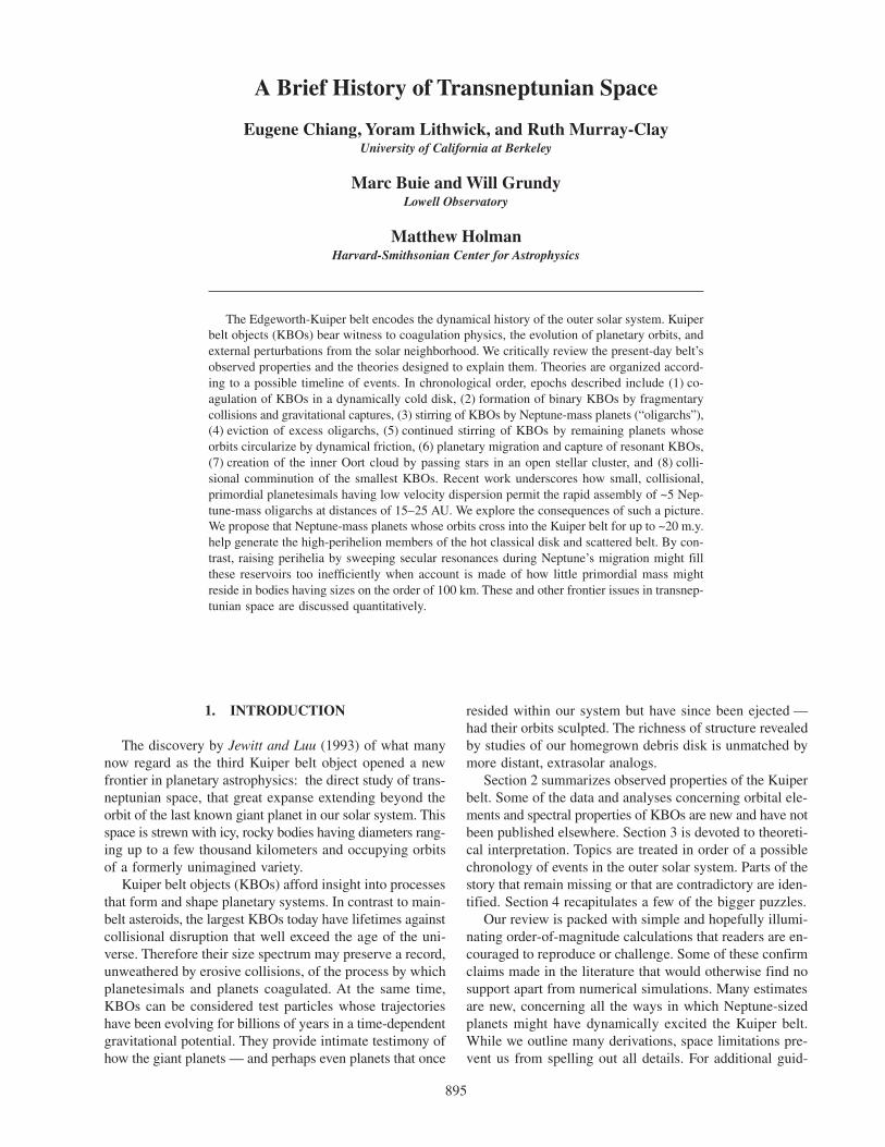
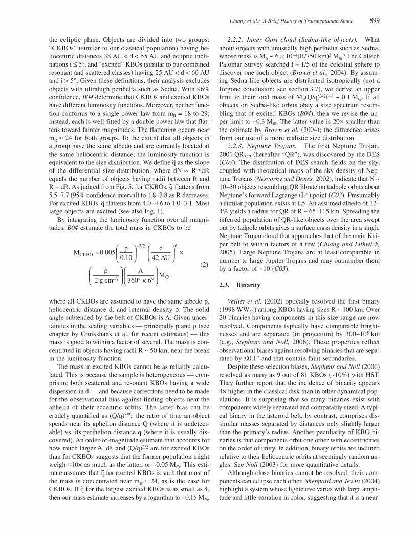
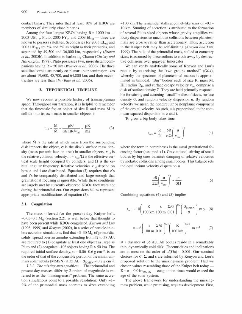
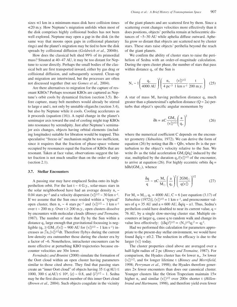
Outer solar system objects divide into dynamical classesbased on how their trajectories evolve. Figure 1 displays or-bital elements, time-averaged over 10 m.y. in a numericalorbit integration that accounts for the masses of the fourgiant planets, of 529 objects. Dynamical classifications ofthese objects are secure according to criteria developed bythe Deep Ecliptic Survey (DES) team (Elliot et al., 2005,hereafter E05). Figure 2 provides a close-up view of a por-tion of the Kuiper belt. We distinguish four classes:

1. Resonant KBOs (122/529) exhibit one or moremean-motion commensurabilities with Neptune, as judgedby steady libration of the appropriate resonance angle(s)

(Chiang et al., 2003, hereafter C03). Resonances mostheavily populated include the exterior 3:2 (Plutino), 2:1, and5:2 (see Table 1). Of special interest is the first discoveredNeptune Trojan (1:1). All resonant KBOs (except the Tro-jan) are found to occupy e-type resonances; the ability ofan e-type resonance to retain a KBO tends to increase withthe KBO’s eccentricity e (e.g., Murray and Dermott, 1999).Unless otherwise stated, orbital elements are heliocentricand referred to the invariable plane. Several (9/122) alsoinhabit inclination-type (i2) or mixed-type (ei2) resonances.None inhabits an eN-type resonance whose stability dependson the (small) eccentricity of Neptune. The latter observa-tion is consistent with numerical experiments that suggesteN-type resonances are rendered unstable by adjacent e-typeresonances.

2. Centaurs (55/529) are nonresonant objects whoseperihelia penetrate inside the orbit of Neptune. Most Cen-taurs cross the Hill sphere of a planet within 10 m.y. Cen-taurs are likely descendants of the other three classes, re-cently dislodged from the Kuiper belt by planetary per-

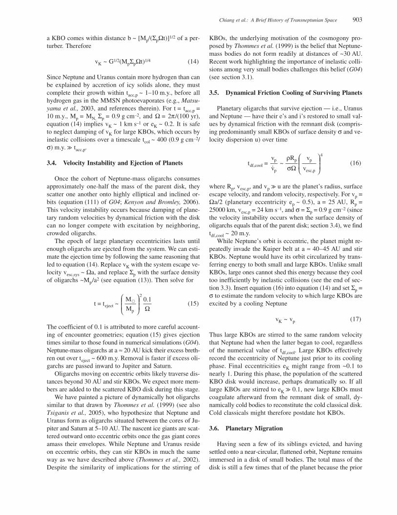
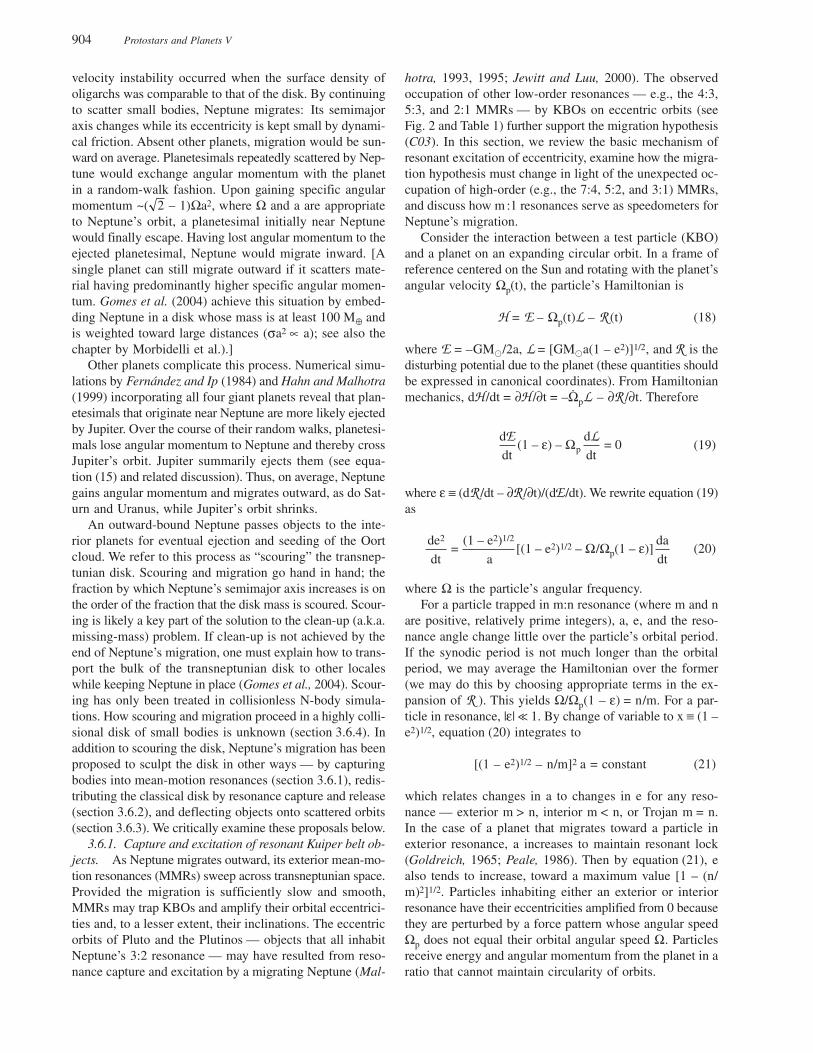
Fig. 1. Orbital elements, time-averaged over 10 m.y., of 529 securely classified outer solar system objects as of October 8, 2005.Symbols represent dynamical classes: Centaurs (×), resonant KBOs ( ), classical KBOs ( ), and scattered KBOs ( ). Dashed verticallines indicate occupied mean-motion resonances; in order of increasing heliocentric distance, these include the 1:1, 5:4, 4:3, 3:2, 5:3,7:4, 9:5, 2:1, 7:3, 5:2, and 3:1 (see Table 1). Solid curves trace loci of constant perihelion q = a(1 – e). Especially large [2003 UB313,Pluto, 2003 EL61, 2005 FY9 (Brown et al., 2005a,b)] and dynamically unusual [2001 QR322 (Trojan) (Chiang et al., 2003; Chiang andLithwick, 2005), 2000 CR105 (high q) (Millis et al., 2002; Gladman et al., 2002), Sedna (high q) (Brown et al., 2004)] KBOs arelabeled. For a zoomed-in view, see Fig. 2.


turbations (Holman and Wisdom, 1993, hereafter HW93;Tiscareno and Malhotra, 2003). They will not be discussedfurther.

3. Classical KBOs (246/529) are nonresonant, nonplanet-crossing objects whose time-averaged ⟨e⟩ ≤ 0.2 and whosetime-averaged Tisserand parameters

(a/aN)(1 – e2) cos ∆i⟩⟨T⟩ = ⟨(aN/a) + 2 (1)

exceed 3. Here ∆i is the mutual inclination between the or-bit planes of Neptune and the KBO, a is the semimajor axisof the KBO, and aN is the semimajor axis of Neptune. Inthe circular, restricted, three-body problem, test particleswith T > 3 and a > aN cannot cross the orbit of the planet[i.e., their perihelia q = a(1 – e) remain greater than aN].Thus, classical KBOs can be argued to have never under-gone close encounters with Neptune in its current nearlycircular orbit and to be relatively pristine dynamically. In-deed, many classical KBOs as identified by our schemehave low inclinations ⟨i⟩ < 5° (“cold classicals”), thoughsome do not (“hot classicals”). Our defining threshold for⟨e⟩ is arbitrary; like our threshold for ⟨T⟩, it is imposed to

suggest — perhaps incorrectly — which KBOs might haveformed and evolved in situ.

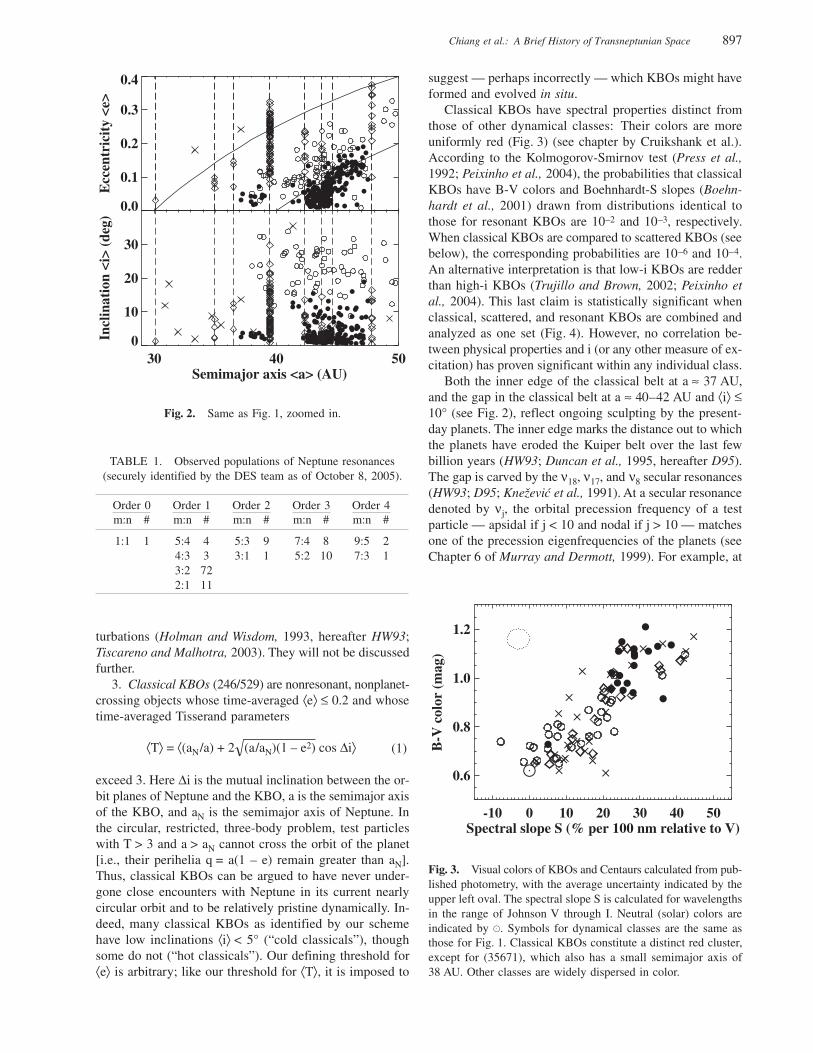
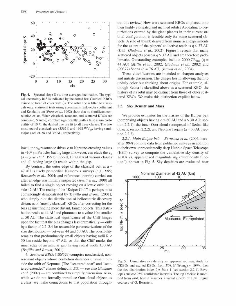
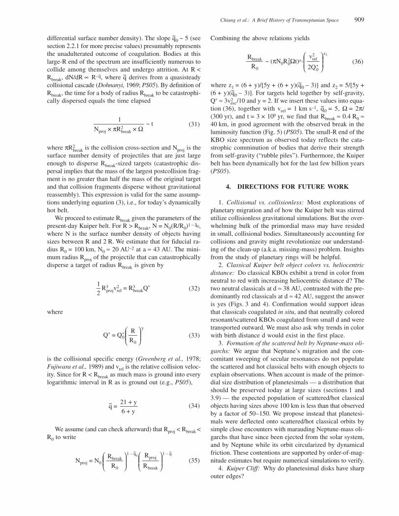
Classical KBOs have spectral properties distinct fromthose of other dynamical classes: Their colors are moreuniformly red (Fig. 3) (see chapter by Cruikshank et al.).According to the Kolmogorov-Smirnov test (Press et al.,1992; Peixinho et al., 2004), the probabilities that classicalKBOs have B-V colors and Boehnhardt-S slopes (Boehn-hardt et al., 2001) drawn from distributions identical tothose for resonant KBOs are 10–2 and 10–3, respectively.When classical KBOs are compared to scattered KBOs (seebelow), the corresponding probabilities are 10–6 and 10–4.An alternative interpretation is that low-i KBOs are redderthan high-i KBOs (Trujillo and Brown, 2002; Peixinho etal., 2004). This last claim is statistically significant whenclassical, scattered, and resonant KBOs are combined andanalyzed as one set (Fig. 4). However, no correlation be-tween physical properties and i (or any other measure of ex-citation) has proven significant within any individual class.

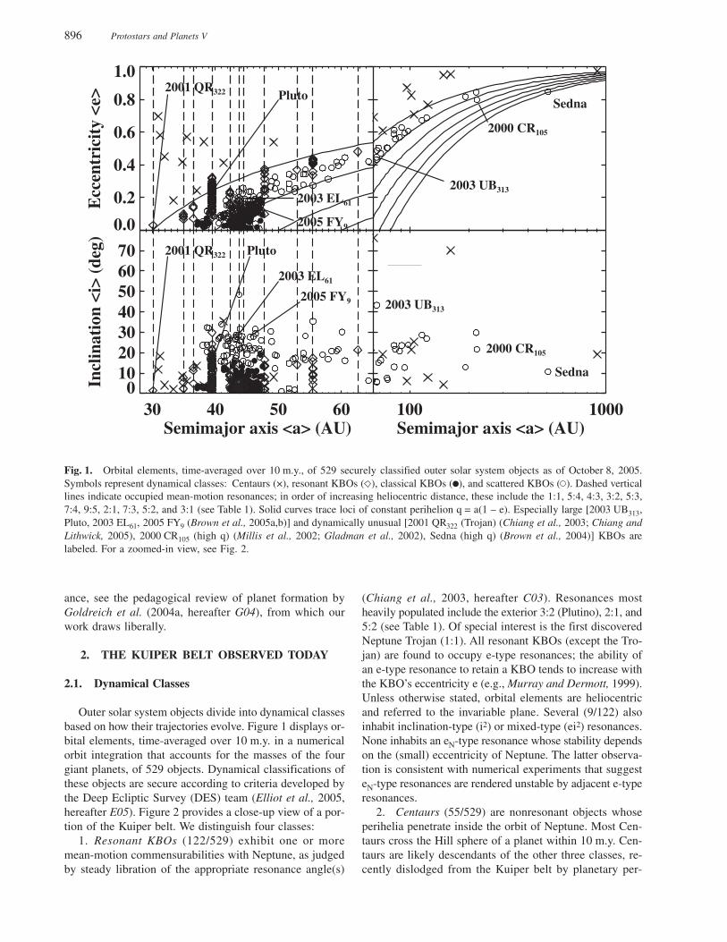
Both the inner edge of the classical belt at a ≈ 37 AU,and the gap in the classical belt at a ≈ 40–42 AU and ⟨i⟩ <10° (see Fig. 2), reflect ongoing sculpting by the present-day planets. The inner edge marks the distance out to whichthe planets have eroded the Kuiper belt over the last fewbillion years (HW93; Duncan et al., 1995, hereafter D95).The gap is carved by the ν18, ν17, and ν8 secular resonances(HW93; D95; Knezevic et al., 1991). At a secular resonancedenoted by νj, the orbital precession frequency of a testparticle — apsidal if j < 10 and nodal if j > 10 — matchesone of the precession eigenfrequencies of the planets (seeChapter 6 of Murray and Dermott, 1999). For example, at

TABLE 1. Observed populations of Neptune resonances(securely identified by the DES team as of October 8, 2005).

Order 0 Order 1 Order 2 Order 3 Order 4m:n # m:n # m:n # m:n # m:n #

1:1 1 5:4 4 5:3 9 7:4 8 9:5 24:3 3 3:1 1 5:2 10 7:3 13:2 722:1 11

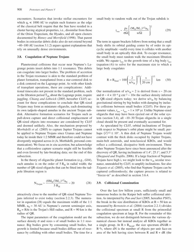
Fig. 2. Same as Fig. 1, zoomed in.

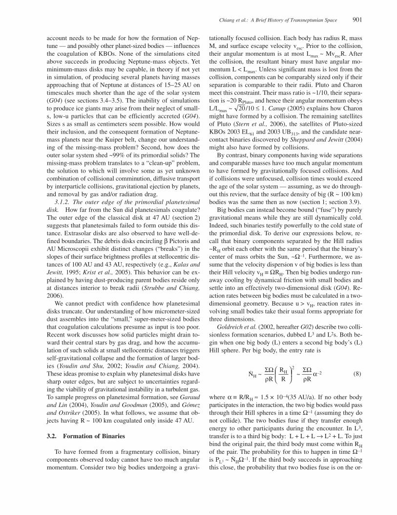
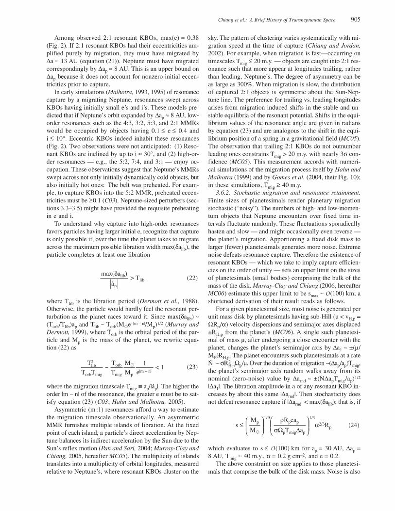
Fig. 3. Visual colors of KBOs and Centaurs calculated from pub-lished photometry, with the average uncertainty indicated by theupper left oval. The spectral slope S is calculated for wavelengthsin the range of Johnson V through I. Neutral (solar) colors areindicated by . Symbols for dynamical classes are the same asthose for Fig. 1. Classical KBOs constitute a distinct red cluster,except for (35671), which also has a small semimajor axis of38 AU. Other classes are widely dispersed in color.


low i, the ν8 resonance drives e to Neptune-crossing valuesin ~106 yr. Particles having large i, however, can elude the ν8(Knezevic et al., 1991). Indeed, 18 KBOs of various classesand all having large ⟨i⟩ reside within the gap.

By contrast, the outer edge of the classical belt at a ≈47 AU is likely primordial. Numerous surveys (e.g., E05;Bernstein et al., 2004; and references therein) carried outafter an edge was initially suspected (Jewitt et al., 1998) allfailed to find a single object moving on a low-e orbit out-side 47 AU. The reality of the “Kuiper Cliff” is perhaps mostconvincingly demonstrated by Trujillo and Brown (2001),who simply plot the distribution of heliocentric discoverydistances of (mostly classical) KBOs after correcting for thebias against finding more distant, fainter objects. This distri-bution peaks at 44 AU and plummets to a value 10× smallerat 50 AU. The statistical significance of the Cliff hingesupon the fact that the bias changes less dramatically — onlyby a factor of 2.2–2.4 for reasonable parameterizations of thesize distribution — between 44 and 50 AU. The possibilityremains that predominantly small objects having radii R <50 km reside beyond 47 AU, or that the Cliff marks theinner edge of an annular gap having radial width >30 AU(Trujillo and Brown, 2001).

4. Scattered KBOs (106/529) comprise nonclassical, non-resonant objects whose perihelion distances q remain out-side the orbit of Neptune. [The “scattered-near” and “scat-tered-extended” classes defined in E05 — see also Gladmanet al. (2002) — are combined to simplify discussion. Also,while we do not formally introduce Oort cloud objects asa class, we make connections to that population through-

out this review.] How were scattered KBOs emplaced ontotheir highly elongated and inclined orbits? Appealing to per-turbations exerted by the giant planets in their current or-bital configuration is feasible only for some scattered ob-jects. A rule of thumb derived from numerical experimentsfor the extent of the planets’ collective reach is q < 37 AU(D95; Gladman et al., 2002). Figure 1 reveals that manyscattered objects possess q > 37 AU and are therefore prob-lematic. Outstanding examples include 2000 CR105 (q =44 AU) (Millis et al., 2002; Gladman et al., 2002) and(90377) Sedna (q = 76 AU) (Brown et al., 2004).

These classifications are intended to sharpen analysesand initiate discussion. The danger lies in allowing them tounduly color our thinking about origins. For example, al-though Sedna is classified above as a scattered KBO, thehistory of its orbit may be distinct from those of other scat-tered KBOs. We make this distinction explicit below.

2.2. Sky Density and Mass

We provide estimates for the masses of the Kuiper belt(comprising objects having q < 60 AU and a > 30 AU; sec-tion 2.2.1); the inner Oort cloud (composed of Sedna-likeobjects; section 2.2.2); and Neptune Trojans (a ≈ 30 AU; sec-tion 2.2.3).

2.2.1. Main Kuiper belt. Bernstein et al. (2004, here-after B04) compile data from published surveys in additionto their own unprecedentedly deep Hubble Space Telescope(HST) survey to compute the cumulative sky density ofKBOs vs. apparent red magnitude mR (“luminosity func-tion”), shown in Fig. 5. Sky densities are evaluated near

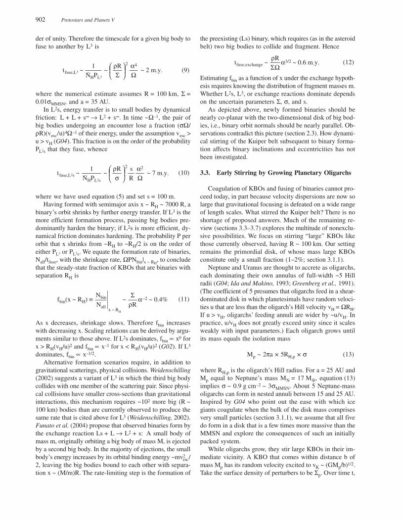
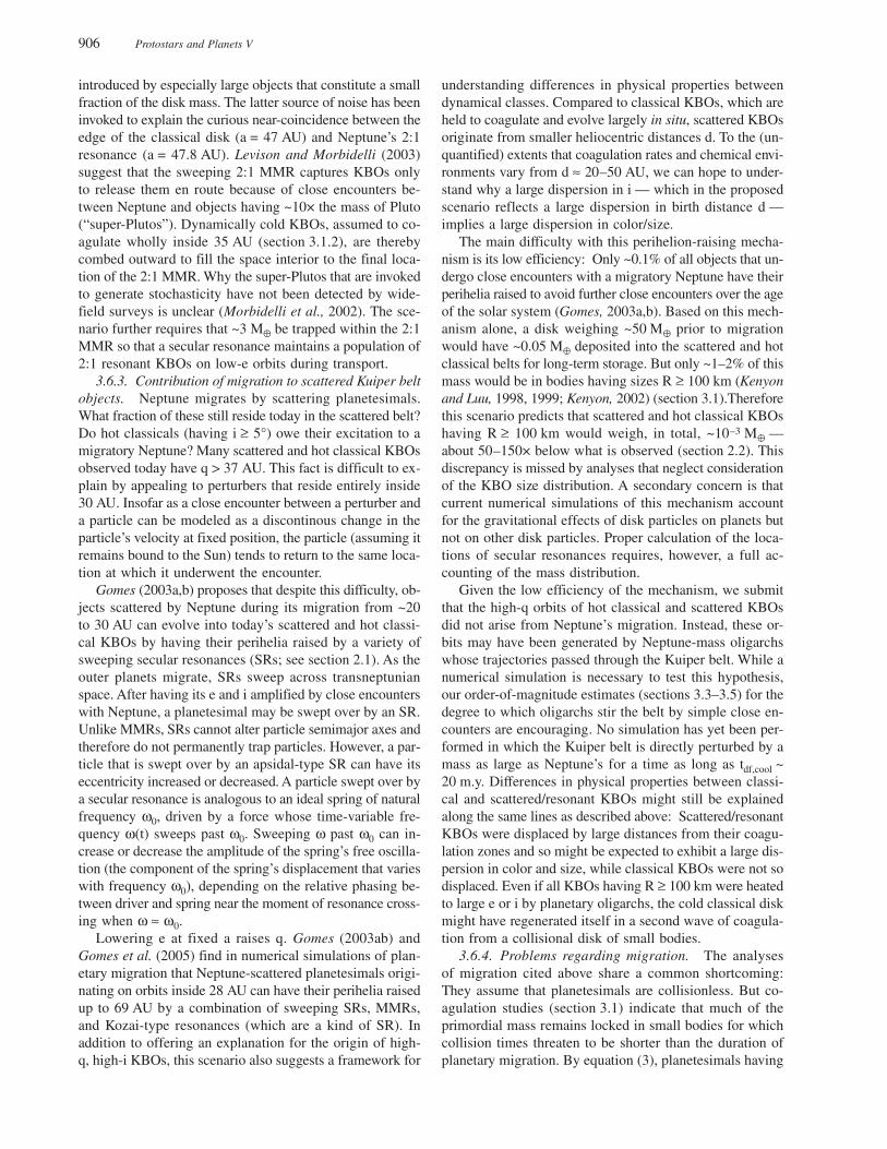
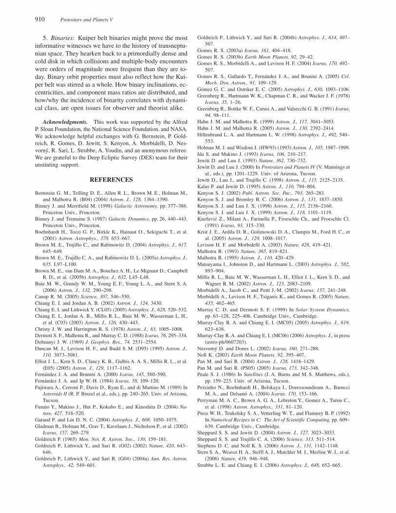
Fig. 4. Spectral slope S vs. time-averaged inclination. The typi-cal uncertainty in S is indicated by the dotted bar. Classical KBOsevince no trend of color with ⟨i⟩. The solid line is fitted to classi-cals only; statistical tests using Spearman’s rank-order coefficientand Kendall’s tau (Press et al., 1992) show that no significant cor-relation exists. When classical, resonant, and scattered KBOs arecombined, S and ⟨i⟩ correlate significantly (with a false alarm prob-ability of 10–5); the dashed line is a fit to all three classes. The twomost neutral classicals are (35671) and 1998 WV24, having semi-major axes of 38 and 39 AU, respectively.

Fig. 5. Cumulative sky density vs. apparent red magnitude forCKBOs and excited KBOs, from B04. If N(<mR) ∝ 10αmR, thenthe size distribution index q~ = 5α + 1 (see section 2.2.1). Enve-lopes enclose 95% confidence intervals. The top abscissa is modi-fied from B04; here it assumes a visual albedo of 10%. Figurecourtesy of G. Bernstein.


the ecliptic plane. Objects are divided into two groups:“CKBOs” (similar to our classical population) having he-liocentric distances 38 AU < d < 55 AU and ecliptic incli-nations i ≤ 5°, and “excited” KBOs (similar to our combinedresonant and scattered classes) having 25 AU < d < 60 AUand i > 5°. Given these definitions, their analysis excludesobjects with ultrahigh perihelia such as Sedna. With 96%confidence, B04 determine that CKBOs and excited KBOshave different luminosity functions. Moreover, neither func-tion conforms to a single power law from mR = 18 to 29;instead, each is well-fitted by a double power law that flat-tens toward fainter magnitudes. The flattening occurs nearmR ≈ 24 for both groups. To the extent that all objects ina group have the same albedo and are currently located atthe same heliocentric distance, the luminosity function isequivalent to the size distribution. We define q~ as the slopeof the differential size distribution, where dN ∝ R–q~dRequals the number of objects having radii between R andR + dR. As judged from Fig. 5, for CKBOs, q~ flattens from5.5–7.7 (95% confidence interval) to 1.8–2.8 as R decreases.For excited KBOs, q~ flattens from 4.0–4.6 to 1.0–3.1. Mostlarge objects are excited (see also Fig. 1).

By integrating the luminosity function over all magni-tudes, B04 estimate the total mass in CKBOs to be

–3/2

ρ

×6

M360° × 6°

A

2 g cm–3

42 AU

d

0.10

pMCKBO ≈ 0.005

(2)

where all CKBOs are assumed to have the same albedo p,heliocentric distance d, and internal density ρ. The solidangle subtended by the belt of CKBOs is A. Given uncer-tainties in the scaling variables — principally p and ρ (seechapter by Cruikshank et al. for recent estimates) — thismass is good to within a factor of several. The mass is con-centrated in objects having radii R ~ 50 km, near the breakin the luminosity function.

The mass in excited KBOs cannot be as reliably calcu-lated. This is because the sample is heterogeneous — com-prising both scattered and resonant KBOs having a widedispersion in d — and because corrections need to be madefor the observational bias against finding objects near theaphelia of their eccentric orbits. The latter bias can becrudely quantified as (Q/q)3/2: the ratio of time an objectspends near its aphelion distance Q (where it is undetect-able) vs. its perihelion distance q (where it is usually dis-covered). An order-of-magnitude estimate that accounts forhow much larger A, d6, and (Q/q)3/2 are for excited KBOsthan for CKBOs suggests that the former population mightweigh ~10× as much as the latter, or ~0.05 M . This esti-mate assumes that q~ for excited KBOs is such that most ofthe mass is concentrated near mR ≈ 24, as is the case forCKBOs. If q~ for the largest excited KBOs is as small as 4,then our mass estimate increases by a logarithm to ~0.15 M .

2.2.2. Inner Oort cloud (Sedna-like objects). Whatabout objects with unusually high perihelia such as Sedna,whose mass is MS ~ 6 × 10–4(R/750 km)3 M ? The CaltechPalomar Survey searched f ~ 1/5 of the celestial sphere todiscover one such object (Brown et al., 2004). By assum-ing Sedna-like objects are distributed isotropically (not aforgone conclusion; see section 3.7), we derive an upperlimit to their total mass of MS(Q/q)3/2f –1 ~ 0.1 M . If allobjects on Sedna-like orbits obey a size spectrum resem-bling that of excited KBOs (B04), then we revise the up-per limit to ~0.3 M . The latter value is 20× smaller thanthe estimate by Brown et al. (2004); the difference arisesfrom our use of a more realistic size distribution.

2.2.3. Neptune Trojans. The first Neptune Trojan,2001 QR322 (hereafter “QR”), was discovered by the DES(C03). The distribution of DES search fields on the sky,coupled with theoretical maps of the sky density of Nep-tune Trojans (Nesvorný and Dones, 2002), indicate that N ~10–30 objects resembling QR librate on tadpole orbits aboutNeptune’s forward Lagrange (L4) point (C03). Presumablya similar population exists at L5. An assumed albedo of 12–4% yields a radius for QR of R ~ 65–115 km. Spreading theinferred population of QR-like objects over the area sweptout by tadpole orbits gives a surface mass density in a singleNeptune Trojan cloud that approaches that of the main Kui-per belt to within factors of a few (Chiang and Lithwick,2005). Large Neptune Trojans are at least comparable innumber to large Jupiter Trojans and may outnumber themby a factor of ~10 (C03).

2.3. Binarity

Veillet et al. (2002) optically resolved the first binary(1998 WW31) among KBOs having sizes R ~ 100 km. Over20 binaries having components in this size range are nowresolved. Components typically have comparable bright-nesses and are separated (in projection) by 300–105 km(e.g., Stephens and Noll, 2006). These properties reflectobservational biases against resolving binaries that are sepa-rated by <0.1" and that contain faint secondaries.

Despite these selection biases, Stephens and Noll (2006)resolved as many as 9 out of 81 KBOs (~10%) with HST.They further report that the incidence of binarity appears4× higher in the classical disk than in other dynamical pop-ulations. It is surprising that so many binaries exist withcomponents widely separated and comparably sized. A typi-cal binary in the asteroid belt, by contrast, comprises dis-similar masses separated by distances only slightly largerthan the primary’s radius. Another peculiarity of KBO bi-naries is that components orbit one other with eccentricitieson the order of unity. In addition, binary orbits are inclinedrelative to their heliocentric orbits at seemingly random an-gles. See Noll (2003) for more quantitative details.

Although close binaries cannot be resolved, their com-ponents can eclipse each other. Sheppard and Jewitt (2004)highlight a system whose lightcurve varies with large ampli-tude and little variation in color, suggesting that it is a near-


contact binary. They infer that at least 10% of KBOs aremembers of similarly close binaries.

Among the four largest KBOs having R ≈ 1000 km —2003 UB313, Pluto, 2005 FY9, and 2003 EL61 — three areknown to possess satellites. Secondaries for 2003 EL61 and2003 UB313 are 5% and 2% as bright as their primaries, andseparated by 49,500 and 36,000 km, respectively (Brownet al., 2005b). In addition to harboring Charon (Christy andHarrington, 1978), Pluto possesses two, more distant com-panions having R ~ 50 km (Weaver et al., 2006). The threesatellites’ orbits are nearly co-planar; their semimajor axesare about 19,600, 48,700, and 64,800 km; and their eccen-tricities are less than 1% (Buie et al., 2006).

3. THEORETICAL TIMELINE

We now recount a possible history of transneptunianspace. Throughout our narration, it is helpful to rememberthat the timescale for an object of size R and mass M tocollide into its own mass in smaller objects is

σΩρRρR3

~(σ/h)R2vrel

~M

Mtcol ~ (3)

where M is the rate at which mass from the surroundingdisk impacts the object, σ is the disk’s surface mass den-sity (mass per unit face-on area) in smaller objects, vrel isthe relative collision velocity, h ~ vrel/Ω is the effective ver-tical scale height occupied by colliders, and Ω is the or-bital angular frequency. Relative velocities vrel depend onhow e and i are distributed. Equation (3) requires that e’sand i’s be comparably distributed and large enough thatgravitational focusing is ignorable. While these conditionsare largely met by currently observed KBOs, they were notduring the primordial era. Our expressions below representappropriate modifications of equation (3).

3.1. Coagulation

The mass inferred for the present-day Kuiper belt,~0.05–0.3 M (section 2.2), is well below that thought tohave been present while KBOs coagulated. Kenyon and Luu(1998, 1999) and Kenyon (2002), in a series of particle-in-a-box accretion simulations, find that ~3–30 M of primordialsolids, spread over an annulus extending from 32 to 38 AU,are required to (1) coagulate at least one object as large asPluto and (2) coagulate ~105 objects having R > 50 km. Therequired initial surface density, σ ~ 0.06–0.6 g cm–2, is onthe order of that of the condensible portion of the minimum-mass solar nebula (MMSN) at 35 AU: σMMSN ~ 0.2 g cm–2.

3.1.1. The missing-mass problem. That primordial andpresent-day masses differ by 2 orders of magnitude is re-ferred to as the “missing-mass” problem. The same accre-tion simulations point to a possible resolution: Only ~1–2% of the primordial mass accretes to sizes exceeding

~100 km. The remainder stalls at comet-like sizes of ~0.1–10 km. Stunting of accretion is attributed to the formationof several Pluto-sized objects whose gravity amplifies ve-locity dispersions so much that collisions between planetesi-mals are erosive rather than accretionary. Thus, accretionin the Kuiper belt may be self-limiting (Kenyon and Luu,1999). The bulk of the primordial mass, stalled at cometarysizes, is assumed by these authors to erode away by destruc-tive collisions over gigayear timescales.

We can verify analytically some of Kenyon and Luu’sresults by exercising the “two-groups method” (G04),whereby the spectrum of planetesimal masses is approxi-mated as bimodal. “Big” bodies each of size R, mass M,Hill radius RH, and surface escape velocity vesc comprise adisk of surface density Σ. They are held primarily responsi-ble for stirring and accreting “small” bodies of size s, surfacedensity σ, and random velocity dispersion u. By randomvelocity we mean the noncircular or nonplanar componentof the orbital velocity. As such, u is proportional to the root-mean-squared dispersion in e and i.

To grow a big body takes time

2

vesc

u~

R

Rtacc ≡ σΩ

ρR(4)

where the term in parentheses is the usual gravitational fo-cussing factor (assumed <1). Gravitational stirring of smallbodies by big ones balances damping of relative velocitiesby inelastic collisions among small bodies. This balance setsthe equilibrium velocity dispersion u

σΩρs

ΣΩρR

~vesc

u4

(5)

Combining equations (4) and (5) implies

m.y.0.01100 m

s

100 km

Rtacc ~ 10

1/2

σσMMSNΣ /σ

(6)

m s–1

100 km

R

0.01100 m

su ~ 6

Σ /σ 1/4 3/4

(7)

at a distance of 35 AU. All bodies reside in a remarkablythin, dynamically cold disk: Eccentricities and inclinationsare at most on the order of u/(Ωa) ~ 0.001. Our nominalchoices for σ, Σ, and s are informed by Kenyon and Luu’sproposed solution to the missing-mass problem. Had wechosen values resembling those of the Kuiper belt today —Σ ~ σ ~ 0.01σMMSN — coagulation times would exceed theage of the solar system.

The above framework for understanding the missing-mass problem, while promising, requires development. First,


account needs to be made for how the formation of Nep-tune — and possibly other planet-sized bodies — influencesthe coagulation of KBOs. None of the simulations citedabove succeeds in producing Neptune-mass objects. Yetminimum-mass disks may be capable, in theory if not yetin simulation, of producing several planets having massesapproaching that of Neptune at distances of 15–25 AU ontimescales much shorter than the age of the solar system(G04) (see sections 3.4–3.5). The inability of simulationsto produce ice giants may arise from their neglect of small-s, low-u particles that can be efficiently accreted (G04).Sizes s as small as centimeters seem possible. How wouldtheir inclusion, and the consequent formation of Neptune-mass planets near the Kuiper belt, change our understand-ing of the missing-mass problem? Second, how does theouter solar system shed ~99% of its primordial solids? Themissing-mass problem translates to a “clean-up” problem,the solution to which will involve some as yet unknowncombination of collisional comminution, diffusive transportby interparticle collisions, gravitational ejection by planets,and removal by gas and/or radiation drag.

3.1.2. The outer edge of the primordial planetesimaldisk. How far from the Sun did planetesimals coagulate?The outer edge of the classical disk at 47 AU (section 2)suggests that planetesimals failed to form outside this dis-tance. Extrasolar disks are also observed to have well-de-fined boundaries. The debris disks encircling β Pictoris andAU Microscopii exhibit distinct changes (“breaks”) in theslopes of their surface brightness profiles at stellocentric dis-tances of 100 AU and 43 AU, respectively (e.g., Kalas andJewitt, 1995; Krist et al., 2005). This behavior can be ex-plained by having dust-producing parent bodies reside onlyat distances interior to break radii (Strubbe and Chiang,2006).

We cannot predict with confidence how planetesimaldisks truncate. Our understanding of how micrometer-sizeddust assembles into the “small,” super-meter-sized bodiesthat coagulation calculations presume as input is too poor.Recent work discusses how solid particles might drain to-ward their central stars by gas drag, and how the accumu-lation of such solids at small stellocentric distances triggersself-gravitational collapse and the formation of larger bod-ies (Youdin and Shu, 2002; Youdin and Chiang, 2004).These ideas promise to explain why planetesimal disks havesharp outer edges, but are subject to uncertainties regard-ing the viability of gravitational instability in a turbulent gas.To sample progress on planetesimal formation, see Garaudand Lin (2004), Youdin and Goodman (2005), and Gómezand Ostriker (2005). In what follows, we assume that ob-jects having R ~ 100 km coagulated only inside 47 AU.

3.2. Formation of Binaries

To have formed from a fragmentary collision, binarycomponents observed today cannot have too much angularmomentum. Consider two big bodies undergoing a gravi-

tationally focused collision. Each body has radius R, massM, and surface escape velocity vesc. Prior to the collision,their angular momentum is at most Lmax ~ MvescR. Afterthe collision, the resultant binary must have angular mo-mentum L < Lmax. Unless significant mass is lost from thecollision, components can be comparably sized only if theirseparation is comparable to their radii. Pluto and Charonmeet this constraint. Their mass ratio is ~1/10, their separa-tion is ~20 RPluto, and hence their angular momentum obeysL/Lmax ~ 20 /10 < 1. Canup (2005) explains how Charonmight have formed by a collision. The remaining satellitesof Pluto (Stern et al., 2006), the satellites of Pluto-sizedKBOs 2003 EL61 and 2003 UB313, and the candidate near-contact binaries discovered by Sheppard and Jewitt (2004)might also have formed by collisions.

By contrast, binary components having wide separationsand comparable masses have too much angular momentumto have formed by gravitationally focused collisions. Andif collisions were unfocused, collision times would exceedthe age of the solar system — assuming, as we do through-out this review, that the surface density of big (R ~ 100 km)bodies was the same then as now (section 1; section 3.9).

Big bodies can instead become bound (“fuse”) by purelygravitational means while they are still dynamically cold.Indeed, such binaries testify powerfully to the cold state ofthe primordial disk. To derive our expressions below, re-call that binary components separated by the Hill radius~RH orbit each other with the same period that the binary’scenter of mass orbits the Sun, ~Ω–1. Furthermore, we as-sume that the velocity dispersion v of big bodies is less thantheir Hill velocity vH ≡ ΩRH. Then big bodies undergo run-away cooling by dynamical friction with small bodies andsettle into an effectively two-dimensional disk (G04). Re-action rates between big bodies must be calculated in a two-dimensional geometry. Because u > vH, reaction rates in-volving small bodies take their usual forms appropriate forthree dimensions.

Goldreich et al. (2002, hereafter G02) describe two colli-sionless formation scenarios, dubbed L3 and L2s. Both be-gin when one big body (L) enters a second big body’s (L)Hill sphere. Per big body, the entry rate is

2

~RHNH ~ α–2

ρR

ΣΩRρR

ΣΩ(8)

where α ≡ R/RH ≈ 1.5 × 10–4(35 AU/a). If no other bodyparticipates in the interaction, the two big bodies would passthrough their Hill spheres in a time Ω–1 (assuming they donot collide). The two bodies fuse if they transfer enoughenergy to other participants during the encounter. In L3,transfer is to a third big body: L + L + L → L2 + L. To justbind the original pair, the third body must come within RHof the pair. The probability for this to happen in time Ω–1

is PL3 ~ NHΩ–1. If the third body succeeds in approachingthis close, the probability that two bodies fuse is on the or-


der of unity. Therefore the timescale for a given big body tofuse to another by L3 is

~ 2 m.y.~NHPL3

1tfuse,L3 ~

2

Ωα4

ΣρR

(9)

where the numerical estimate assumes R = 100 km, Σ =0.01σMMSN, and a = 35 AU.

In L2s, energy transfer is to small bodies by dynamicalfriction: L + L + s∞ → L2 + s∞. In time ~Ω–1, the pair ofbig bodies undergoing an encounter lose a fraction (σΩ/ρR)(vesc/u)4Ω–1 of their energy, under the assumption vesc >u > vH (G04). This fraction is on the order of the probabilityPL2s that they fuse, whence

~ 7 m.y.~NHPL2s

1tfuse,L2s ~

2

Ωα2

R

s

σρR

(10)

where we have used equation (5) and set s = 100 m.Having formed with semimajor axis x ~ RH ~ 7000 R, a

binary’s orbit shrinks by further energy transfer. If L3 is themore efficient formation process, passing big bodies pre-dominantly harden the binary; if L2s is more efficient, dy-namical friction dominates hardening. The probability P perorbit that x shrinks from ~RH to ~RH/2 is on the order ofeither PL3 or PL2s. We equate the formation rate of binaries,Nall/tfuse, with the shrinkage rate, ΩPNbin|x ~ RH

, to concludethat the steady-state fraction of KBOs that are binaries withseparation RH is

~Nall

Nbinfbin(x ~ RH) ≡x ~ RH

α–2 ~ 0.4%ρR

Σ(11)

As x decreases, shrinkage slows. Therefore fbin increaseswith decreasing x. Scaling relations can be derived by argu-ments similar to those above. If L2s dominates, fbin ∝ x0 forx > RH(vH/u)2 and fbin ∝ x–1 for x < RH(vH/u)2 (G02). If L3

dominates, fbin ∝ x–1/2.Alternative formation scenarios require, in addition to

gravitational scatterings, physical collisions. Weidenschilling(2002) suggests a variant of L3 in which the third big bodycollides with one member of the scattering pair. Since physi-cal collisions have smaller cross-sections than gravitationalinteractions, this mechanism requires ~102 more big (R ~100 km) bodies than are currently observed to produce thesame rate that is cited above for L3 (Weidenschilling, 2002).Funato et al. (2004) propose that observed binaries form bythe exchange reaction Ls + L → L2 + s: A small body ofmass m, originally orbiting a big body of mass M, is ejectedby a second big body. In the majority of ejections, the smallbody’s energy increases by its orbital binding energy ~mv2

esc/2, leaving the big bodies bound to each other with separa-tion x ~ (M/m)R. The rate-limiting step is the formation of

the preexisting (Ls) binary, which requires (as in the asteroidbelt) two big bodies to collide and fragment. Hence

tfuse,exchange ~ α3/2 ~ 0.6 m.y.ΣΩρR

(12)

Estimating fbin as a function of x under the exchange hypoth-esis requires knowing the distribution of fragment masses m.Whether L2s, L3, or exchange reactions dominate dependson the uncertain parameters Σ, σ, and s.

As depicted above, newly formed binaries should benearly co-planar with the two-dimensional disk of big bod-ies, i.e., binary orbit normals should be nearly parallel. Ob-servations contradict this picture (section 2.3). How dynami-cal stirring of the Kuiper belt subsequent to binary forma-tion affects binary inclinations and eccentricities has notbeen investigated.

3.3. Early Stirring by Growing Planetary Oligarchs

Coagulation of KBOs and fusing of binaries cannot pro-ceed today, in part because velocity dispersions are now solarge that gravitational focusing is defeated on a wide rangeof length scales. What stirred the Kuiper belt? There is noshortage of proposed answers. Much of the remaining re-view (sections 3.3–3.7) explores the multitude of nonexclu-sive possibilities. We focus on stirring “large” KBOs likethose currently observed, having R ~ 100 km. Our settingremains the primordial disk, of whose mass large KBOsconstitute only a small fraction (1–2%; section 3.1.1).

Neptune and Uranus are thought to accrete as oligarchs,each dominating their own annulus of full-width ~5 Hillradii (G04; Ida and Makino, 1993; Greenberg et al., 1991).(The coefficient of 5 presumes that oligarchs feed in a shear-dominated disk in which planetesimals have random veloci-ties u that are less than the oligarch’s Hill velocity vH = ΩRH.If u > vH, oligarchs’ feeding annuli are wider by ~u/vH. Inpractice, u/vH does not greatly exceed unity since it scalesweakly with input parameters.) Each oligarch grows untilits mass equals the isolation mass

Mp ~ 2πa × 5RH,p × σ (13)

where RH,p is the oligarch’s Hill radius. For a = 25 AU andMp equal to Neptune’s mass MN = 17 M , equation (13)implies σ ~ 0.9 g cm–2 ~ 3σMMSN. About 5 Neptune-massoligarchs can form in nested annuli between 15 and 25 AU.Inspired by G04 who point out the ease with which icegiants coagulate when the bulk of the disk mass comprisesvery small particles (section 3.1.1), we assume that all fivedo form in a disk that is a few times more massive than theMMSN and explore the consequences of such an initiallypacked system.

While oligarchs grow, they stir large KBOs in their im-mediate vicinity. A KBO that comes within distance b ofmass Mp has its random velocity excited to vK ~ (GMp/b)1/2.Take the surface density of perturbers to be Σp. Over time t,


a KBO comes within distance b ~ [Mp/(ΣpΩt)]1/2 of a per-turber. Therefore

vK ~ G1/2(MpΣpΩt)1/4 (14)

Since Neptune and Uranus contain more hydrogen than canbe explained by accretion of icy solids alone, they mustcomplete their growth within tacc,p ~ 1–10 m.y., before allhydrogen gas in the MMSN photoevaporates (e.g., Matsu-yama et al., 2003, and references therein). For t = tacc,p =10 m.y., Mp = MN, Σp = 0.9 g cm–2, and Ω = 2π/(100 yr),equation (14) implies vK ~ 1 km s–1 or eK ~ 0.2. It is safeto neglect damping of vK for large KBOs, which occurs byinelastic collisions over a timescale tcol ~ 400 (0.9 g cm–2/σ) m.y. >> tacc,p.

3.4. Velocity Instability and Ejection of Planets

Once the cohort of Neptune-mass oligarchs consumesapproximately one-half the mass of the parent disk, theyscatter one another onto highly elliptical and inclined or-bits (equation (111) of G04; Kenyon and Bromley, 2006).This velocity instability occurs because damping of plane-tary random velocities by dynamical friction with the diskcan no longer compete with excitation by neighboring,crowded oligarchs.

The epoch of large planetary eccentricities lasts untilenough oligarchs are ejected from the system. We can esti-mate the ejection time by following the same reasoning thatled to equation (14). Replace vK with the system escape ve-locity vesc,sys ~ Ωa, and replace Σp with the surface densityof oligarchs ~Mp/a2 (see equation (13)). Then solve for

Ω0.1

Mp

Mt = teject ~

2

(15)

The coefficient of 0.1 is attributed to more careful account-ing of encounter geometries; equation (15) gives ejectiontimes similar to those found in numerical simulations (G04).Neptune-mass oligarchs at a ≈ 20 AU kick their excess breth-ren out over teject ~ 600 m.y. Removal is faster if excess oli-garchs are passed inward to Jupiter and Saturn.

Oligarchs moving on eccentric orbits likely traverse dis-tances beyond 30 AU and stir KBOs. We expect more mem-bers are added to the scattered KBO disk during this stage.

We have painted a picture of dynamically hot oligarchssimilar to that drawn by Thommes et al. (1999) (see alsoTsiganis et al., 2005), who hypothesize that Neptune andUranus form as oligarchs situated between the cores of Ju-piter and Saturn at 5–10 AU. The nascent ice giants are scat-tered outward onto eccentric orbits once the gas giant coresamass their envelopes. While Neptune and Uranus resideon eccentric orbits, they can stir KBOs in much the sameway as we have described above (Thommes et al., 2002).Despite the similarity of implications for the stirring of

KBOs, the underlying motivation of the cosmogony pro-posed by Thommes et al. (1999) is the belief that Neptune-mass bodies do not form readily at distances of ~30 AU.Recent work highlighting the importance of inelastic colli-sions among very small bodies challenges this belief (G04)(see section 3.1).

3.5. Dynamical Friction Cooling of Surviving Planets

Planetary oligarchs that survive ejection — i.e., Uranusand Neptune — have their e’s and i’s restored to small val-ues by dynamical friction with the remnant disk (compris-ing predominantly small KBOs of surface density σ and ve-locity dispersion u) over time

4

vesc,p

vp~vp

vptdf,cool = σΩρRp (16)

where Rp, vesc,p, and vp >> u are the planet’s radius, surfaceescape velocity, and random velocity, respectively. For vp =Ωa/2 (planetary eccentricity ep ~ 0.5), a = 25 AU, Rp =25000 km, vesc,p = 24 km s–1, and σ = Σp = 0.9 g cm–2 (sincethe velocity instability occurs when the surface density ofoligarchs equals that of the parent disk; section 3.4), we findtdf,cool ~ 20 m.y.

While Neptune’s orbit is eccentric, the planet might re-peatedly invade the Kuiper belt at a ≈ 40–45 AU and stirKBOs. Neptune would have its orbit circularized by trans-ferring energy to both small and large KBOs. Unlike smallKBOs, large ones cannot shed this energy because they cooltoo inefficiently by inelastic collisions (see the end of sec-tion 3.3). Insert equation (16) into equation (14) and set Σp =σ to estimate the random velocity to which large KBOs areexcited by a cooling Neptune

vK ~ vp (17)

Thus large KBOs are stirred to the same random velocitythat Neptune had when the latter began to cool, regardlessof the numerical value of tdf,cool. Large KBOs effectivelyrecord the eccentricity of Neptune just prior to its coolingphase. Final eccentricities eK might range from ~0.1 tonearly 1. During this phase, the population of the scatteredKBO disk would increase, perhaps dramatically so. If alllarge KBOs are stirred to eK >> 0.1, new large KBOs mustcoagulate afterward from the remnant disk of small, dy-namically cold bodies to reconstitute the cold classical disk.Cold classicals might therefore postdate hot KBOs.

3.6. Planetary Migration

Having seen a few of its siblings evicted, and havingsettled onto a near-circular, flattened orbit, Neptune remainsimmersed in a disk of small bodies. The total mass of thedisk is still a few times that of the planet because the prior


velocity instability occurred when the surface density ofoligarchs was comparable to that of the disk. By continuingto scatter small bodies, Neptune migrates: Its semimajoraxis changes while its eccentricity is kept small by dynami-cal friction. Absent other planets, migration would be sun-ward on average. Planetesimals repeatedly scattered by Nep-tune would exchange angular momentum with the planetin a random-walk fashion. Upon gaining specific angularmomentum ~( 2 – 1)Ωa2, where Ω and a are appropriateto Neptune’s orbit, a planetesimal initially near Neptunewould finally escape. Having lost angular momentum to theejected planetesimal, Neptune would migrate inward. [Asingle planet can still migrate outward if it scatters mate-rial having predominantly higher specific angular momen-tum. Gomes et al. (2004) achieve this situation by embed-ding Neptune in a disk whose mass is at least 100 M andis weighted toward large distances (σa2 ∝ a); see also thechapter by Morbidelli et al.).]

Other planets complicate this process. Numerical simu-lations by Fernández and Ip (1984) and Hahn and Malhotra(1999) incorporating all four giant planets reveal that plan-etesimals that originate near Neptune are more likely ejectedby Jupiter. Over the course of their random walks, planetesi-mals lose angular momentum to Neptune and thereby crossJupiter’s orbit. Jupiter summarily ejects them (see equa-tion (15) and related discussion). Thus, on average, Neptunegains angular momentum and migrates outward, as do Sat-urn and Uranus, while Jupiter’s orbit shrinks.

An outward-bound Neptune passes objects to the inte-rior planets for eventual ejection and seeding of the Oortcloud. We refer to this process as “scouring” the transnep-tunian disk. Scouring and migration go hand in hand; thefraction by which Neptune’s semimajor axis increases is onthe order of the fraction that the disk mass is scoured. Scour-ing is likely a key part of the solution to the clean-up (a.k.a.missing-mass) problem. If clean-up is not achieved by theend of Neptune’s migration, one must explain how to trans-port the bulk of the transneptunian disk to other localeswhile keeping Neptune in place (Gomes et al., 2004). Scour-ing has only been treated in collisionless N-body simula-tions. How scouring and migration proceed in a highly colli-sional disk of small bodies is unknown (section 3.6.4). Inaddition to scouring the disk, Neptune’s migration has beenproposed to sculpt the disk in other ways — by capturingbodies into mean-motion resonances (section 3.6.1), redis-tributing the classical disk by resonance capture and release(section 3.6.2), and deflecting objects onto scattered orbits(section 3.6.3). We critically examine these proposals below.

3.6.1. Capture and excitation of resonant Kuiper belt ob-jects. As Neptune migrates outward, its exterior mean-mo-tion resonances (MMRs) sweep across transneptunian space.Provided the migration is sufficiently slow and smooth,MMRs may trap KBOs and amplify their orbital eccentrici-ties and, to a lesser extent, their inclinations. The eccentricorbits of Pluto and the Plutinos — objects that all inhabitNeptune’s 3:2 resonance — may have resulted from reso-nance capture and excitation by a migrating Neptune (Mal-

hotra, 1993, 1995; Jewitt and Luu, 2000). The observedoccupation of other low-order resonances — e.g., the 4:3,5:3, and 2:1 MMRs — by KBOs on eccentric orbits (seeFig. 2 and Table 1) further support the migration hypothesis(C03). In this section, we review the basic mechanism ofresonant excitation of eccentricity, examine how the migra-tion hypothesis must change in light of the unexpected oc-cupation of high-order (e.g., the 7:4, 5:2, and 3:1) MMRs,and discuss how m :1 resonances serve as speedometers forNeptune’s migration.

Consider the interaction between a test particle (KBO)and a planet on an expanding circular orbit. In a frame ofreference centered on the Sun and rotating with the planet’sangular velocity Ωp(t), the particle’s Hamiltonian is

H = E – Ωp(t)L – R (t) (18)

where E = –GM /2a, L = [GM a(1 – e2)]1/2, and R is thedisturbing potential due to the planet (these quantities shouldbe expressed in canonical coordinates). From Hamiltonianmechanics, dH /dt = ∂H /∂t = –Ω

. pL – ∂R /∂t. Therefore

dt

dL(1 – ε) – Ωpdt

dE= 0 (19)

where ε ≡ (dR /dt – ∂R /∂t)/(dE /dt). We rewrite equation (19)as

dt

da[(1 – e2)1/2 – Ω/Ωp(1 – ε)]

a

(1 – e2)1/2

dt

de2= (20)

where Ω is the particle’s angular frequency.For a particle trapped in m:n resonance (where m and n

are positive, relatively prime integers), a, e, and the reso-nance angle change little over the particle’s orbital period.If the synodic period is not much longer than the orbitalperiod, we may average the Hamiltonian over the former(we may do this by choosing appropriate terms in the ex-pansion of R ). This yields Ω/Ωp(1 – ε) = n/m. For a par-ticle in resonance, |ε| << 1. By change of variable to x ≡ (1 –e2)1/2, equation (20) integrates to

[(1 – e2)1/2 – n/m]2 a = constant (21)

which relates changes in a to changes in e for any reso-nance — exterior m > n, interior m < n, or Trojan m = n.In the case of a planet that migrates toward a particle inexterior resonance, a increases to maintain resonant lock(Goldreich, 1965; Peale, 1986). Then by equation (21), ealso tends to increase, toward a maximum value [1 – (n/m)2]1/2. Particles inhabiting either an exterior or interiorresonance have their eccentricities amplified from 0 becausethey are perturbed by a force pattern whose angular speedΩp does not equal their orbital angular speed Ω. Particlesreceive energy and angular momentum from the planet in aratio that cannot maintain circularity of orbits.


Among observed 2:1 resonant KBOs, max(e) ≈ 0.38(Fig. 2). If 2:1 resonant KBOs had their eccentricities am-plified purely by migration, they must have migrated by∆a ≈ 13 AU (equation (21)). Neptune must have migratedcorrespondingly by ∆ap ≈ 8 AU. This is an upper bound on∆ap because it does not account for nonzero initial eccen-tricities prior to capture.

In early simulations (Malhotra, 1993, 1995) of resonancecapture by a migrating Neptune, resonances swept acrossKBOs having initially small e’s and i’s. These models pre-dicted that if Neptune’s orbit expanded by ∆ap ≈ 8 AU, low-order resonances such as the 4:3, 3:2, 5:3, and 2:1 MMRswould be occupied by objects having 0.1 < e < 0.4 andi < 10°. Eccentric KBOs indeed inhabit these resonances(Fig. 2). Two observations were not anticipated: (1) Reso-nant KBOs are inclined by up to i ≈ 30°, and (2) high-or-der resonances — e.g., the 5:2, 7:4, and 3:1 — enjoy oc-cupation. These observations suggest that Neptune’s MMRsswept across not only initially dynamically cold objects, butalso initially hot ones: The belt was preheated. For exam-ple, to capture KBOs into the 5:2 MMR, preheated eccen-tricities must be >0.1 (C03). Neptune-sized perturbers (sec-tions 3.3–3.5) might have provided the requisite preheatingin e and i.

To understand why capture into high-order resonancesfavors particles having larger initial e, recognize that captureis only possible if, over the time the planet takes to migrateacross the maximum possible libration width max(δalib), theparticle completes at least one libration

ap

max(δalib) > Tlib (22)

where Tlib is the libration period (Dermott et al., 1988).Otherwise, the particle would hardly feel the resonant per-turbation as the planet races toward it. Since max(δalib) ~(Torb/Tlib)ap and Tlib ~ Torb(M e–|m – n|/Mp)1/2 (Murray andDermott, 1999), where Torb is the orbital period of the par-ticle and Mp is the mass of the planet, we rewrite equa-tion (22) as

e|m – n|

1

Mp

M

Tmig

Torb~TorbTmig

T2lib < 1 (23)

where the migration timescale Tmig ≡ ap/|ap|. The higher theorder |m – n| of the resonance, the greater e must be to sat-isfy equation (23) (C03; Hahn and Malhotra, 2005).

Asymmetric (m :1) resonances afford a way to estimatethe migration timescale observationally. An asymmetricMMR furnishes multiple islands of libration. At the fixedpoint of each island, a particle’s direct acceleration by Nep-tune balances its indirect acceleration by the Sun due to theSun’s reflex motion (Pan and Sari, 2004; Murray-Clay andChiang, 2005, hereafter MC05). The multiplicity of islandstranslates into a multiplicity of orbital longitudes, measuredrelative to Neptune’s, where resonant KBOs cluster on the

sky. The pattern of clustering varies systematically with mi-gration speed at the time of capture (Chiang and Jordan,2002). For example, when migration is fast—occurring ontimescales Tmig < 20 m.y. — objects are caught into 2:1 res-onance such that more appear at longitudes trailing, ratherthan leading, Neptune’s. The degree of asymmetry can beas large as 300%. When migration is slow, the distributionof captured 2:1 objects is symmetric about the Sun-Nep-tune line. The preference for trailing vs. leading longitudesarises from migration-induced shifts in the stable and un-stable equilibria of the resonant potential. Shifts in the equi-librium values of the resonance angle are given in radiansby equation (23) and are analogous to the shift in the equi-librium position of a spring in a gravitational field (MC05).The observation that trailing 2:1 KBOs do not outnumberleading ones constrains Tmig > 20 m.y. with nearly 3σ con-fidence (MC05). This measurement accords with numeri-cal simulations of the migration process itself by Hahn andMalhotra (1999) and by Gomes et al. (2004, their Fig. 10);in these simulations, Tmig > 40 m.y.

3.6.2. Stochastic migration and resonance retainment.Finite sizes of planetesimals render planetary migrationstochastic (“noisy”). The numbers of high- and low-momen-tum objects that Neptune encounters over fixed time in-tervals fluctuate randomly. These fluctuations sporadicallyhasten and slow — and might occasionally even reverse —the planet’s migration. Apportioning a fixed disk mass tolarger (fewer) planetesimals generates more noise. Extremenoise defeats resonance capture. Therefore the existence ofresonant KBOs — which we take to imply capture efficien-cies on the order of unity — sets an upper limit on the sizesof planetesimals (small bodies) comprising the bulk of themass of the disk. Murray-Clay and Chiang (2006, hereafterMC06) estimate this upper limit to be smax ~ O (100) km; ashortened derivation of their result reads as follows.

For a given planetesimal size, most noise is generated perunit mass disk by planetesimals having sub-Hill (u < vH,p =ΩRp/α) velocity dispersions and semimajor axes displaced±RH,p from the planet’s (MC06). A single such planetesi-mal of mass µ, after undergoing a close encounter with theplanet, changes the planet’s semimajor axis by ∆a1 ~ ±(µ/MP)RH,p. The planet encounters such planetesimals at a rateN ~ σR2

H,pΩp/µ. Over the duration of migration ~(∆ap/ap)Tmig,the planet’s semimajor axis random walks away from itsnominal (zero-noise) value by ∆arnd ~ ±(N∆apTmig/ap)1/2

|∆a1|. The libration amplitude in a of any resonant KBO in-creases by about this same |∆arnd|. Then stochasticity doesnot defeat resonance capture if |∆arnd| < max(δalib); that is, if

1/9 1/3

M

Mps < α2/3RpσΩpTmig∆ap

ρRpeap (24)

which evaluates to s < O (100) km for ap = 30 AU, ∆ap =8 AU, Tmig ≈ 40 m.y., σ = 0.2 g cm–2, and e = 0.2.

The above constraint on size applies to those planetesi-mals that comprise the bulk of the disk mass. Noise is also


introduced by especially large objects that constitute a smallfraction of the disk mass. The latter source of noise has beeninvoked to explain the curious near-coincidence between theedge of the classical disk (a = 47 AU) and Neptune’s 2:1resonance (a = 47.8 AU). Levison and Morbidelli (2003)suggest that the sweeping 2:1 MMR captures KBOs onlyto release them en route because of close encounters be-tween Neptune and objects having ~10× the mass of Pluto(“super-Plutos”). Dynamically cold KBOs, assumed to co-agulate wholly inside 35 AU (section 3.1.2), are therebycombed outward to fill the space interior to the final loca-tion of the 2:1 MMR. Why the super-Plutos that are invokedto generate stochasticity have not been detected by wide-field surveys is unclear (Morbidelli et al., 2002). The sce-nario further requires that ~3 M be trapped within the 2:1MMR so that a secular resonance maintains a population of2:1 resonant KBOs on low-e orbits during transport.

3.6.3. Contribution of migration to scattered Kuiper beltobjects. Neptune migrates by scattering planetesimals.What fraction of these still reside today in the scattered belt?Do hot classicals (having i > 5°) owe their excitation to amigratory Neptune? Many scattered and hot classical KBOsobserved today have q > 37 AU. This fact is difficult to ex-plain by appealing to perturbers that reside entirely inside30 AU. Insofar as a close encounter between a perturber anda particle can be modeled as a discontinous change in theparticle’s velocity at fixed position, the particle (assuming itremains bound to the Sun) tends to return to the same loca-tion at which it underwent the encounter.

Gomes (2003a,b) proposes that despite this difficulty, ob-jects scattered by Neptune during its migration from ~20to 30 AU can evolve into today’s scattered and hot classi-cal KBOs by having their perihelia raised by a variety ofsweeping secular resonances (SRs; see section 2.1). As theouter planets migrate, SRs sweep across transneptunianspace. After having its e and i amplified by close encounterswith Neptune, a planetesimal may be swept over by an SR.Unlike MMRs, SRs cannot alter particle semimajor axes andtherefore do not permanently trap particles. However, a par-ticle that is swept over by an apsidal-type SR can have itseccentricity increased or decreased. A particle swept over bya secular resonance is analogous to an ideal spring of naturalfrequency ω0, driven by a force whose time-variable fre-quency ω(t) sweeps past ω0. Sweeping ω past ω0 can in-crease or decrease the amplitude of the spring’s free oscilla-tion (the component of the spring’s displacement that varieswith frequency ω0), depending on the relative phasing be-tween driver and spring near the moment of resonance cross-ing when ω ≈ ω0.

Lowering e at fixed a raises q. Gomes (2003ab) andGomes et al. (2005) find in numerical simulations of plan-etary migration that Neptune-scattered planetesimals origi-nating on orbits inside 28 AU can have their perihelia raisedup to 69 AU by a combination of sweeping SRs, MMRs,and Kozai-type resonances (which are a kind of SR). Inaddition to offering an explanation for the origin of high-q, high-i KBOs, this scenario also suggests a framework for

understanding differences in physical properties betweendynamical classes. Compared to classical KBOs, which areheld to coagulate and evolve largely in situ, scattered KBOsoriginate from smaller heliocentric distances d. To the (un-quantified) extents that coagulation rates and chemical envi-ronments vary from d ≈ 20–50 AU, we can hope to under-stand why a large dispersion in i — which in the proposedscenario reflects a large dispersion in birth distance d —implies a large dispersion in color/size.

The main difficulty with this perihelion-raising mecha-nism is its low efficiency: Only ~0.1% of all objects that un-dergo close encounters with a migratory Neptune have theirperihelia raised to avoid further close encounters over the ageof the solar system (Gomes, 2003a,b). Based on this mech-anism alone, a disk weighing ~50 M prior to migrationwould have ~0.05 M deposited into the scattered and hotclassical belts for long-term storage. But only ~1–2% of thismass would be in bodies having sizes R > 100 km (Kenyonand Luu, 1998, 1999; Kenyon, 2002) (section 3.1).Thereforethis scenario predicts that scattered and hot classical KBOshaving R > 100 km would weigh, in total, ~10–3 M —about 50–150× below what is observed (section 2.2). Thisdiscrepancy is missed by analyses that neglect considerationof the KBO size distribution. A secondary concern is thatcurrent numerical simulations of this mechanism accountfor the gravitational effects of disk particles on planets butnot on other disk particles. Proper calculation of the loca-tions of secular resonances requires, however, a full ac-counting of the mass distribution.

Given the low efficiency of the mechanism, we submitthat the high-q orbits of hot classical and scattered KBOsdid not arise from Neptune’s migration. Instead, these or-bits may have been generated by Neptune-mass oligarchswhose trajectories passed through the Kuiper belt. While anumerical simulation is necessary to test this hypothesis,our order-of-magnitude estimates (sections 3.3–3.5) for thedegree to which oligarchs stir the belt by simple close en-counters are encouraging. No simulation has yet been per-formed in which the Kuiper belt is directly perturbed by amass as large as Neptune’s for a time as long as tdf,cool ~20 m.y. Differences in physical properties between classi-cal and scattered/resonant KBOs might still be explainedalong the same lines as described above: Scattered/resonantKBOs were displaced by large distances from their coagu-lation zones and so might be expected to exhibit a large dis-persion in color and size, while classical KBOs were not sodisplaced. Even if all KBOs having R > 100 km were heatedto large e or i by planetary oligarchs, the cold classical diskmight have regenerated itself in a second wave of coagula-tion from a collisional disk of small bodies.

3.6.4. Problems regarding migration. The analysesof migration cited above share a common shortcoming:They assume that planetesimals are collisionless. But co-agulation studies (section 3.1) indicate that much of theprimordial mass remains locked in small bodies for whichcollision times threaten to be shorter than the duration ofplanetary migration. By equation (3), planetesimals having


sizes <<1 km in a minimum-mass disk have collision times<<20 m.y. How Neptune’s migration unfolds when most ofthe disk comprises highly collisional bodies has not beenwell explored. Neptune may open a gap in the disk (in thesame way that moons open gaps in collisional planetaryrings) and the planet’s migration may be tied to how the diskspreads by collisional diffusion (Goldreich et al., 2004b).

How does the classical belt shed 99% of its primordialmass? Situated at 40–47 AU, it may be too distant for Nep-tune to scour directly. Perhaps the small bodies of the clas-sical belt are first transported inward, either by gas drag orcollisional diffusion, and subsequently scoured. Clean-upand migration are intertwined, but the processes are oftennot discussed together (but see Gomes et al., 2004).

Are there alternatives to migration for the capture of res-onant KBOs? Perhaps resonant KBOs are captured as Nep-tune’s orbit cools by dynamical friction (section 3.5). Be-fore capture, many belt members would already be stirredto large e and i, not only by unstable oligarchs (section 3.4),but also by Neptune while it cools. Cooling accelerates asit proceeds (equation (16)). A rapid change in the planet’ssemimajor axis toward the end of cooling might trap KBOsinto resonance by serendipity. Just after Neptune’s semima-jor axis changes, objects having orbital elements (includ-ing longitudes) suitable for libration would be trapped. Thisspeculative “freeze-in” mechanism might be too inefficient,since it requires that the fraction of phase-space volumeoccupied by resonances equal the fraction of KBOs that areresonant. Taken at face value, observations suggest the lat-ter fraction is not much smaller than on the order of unity(section 2.1).

3.7. Stellar Encounters

A passing star may have emplaced Sedna onto its high-perihelion orbit. For the last t ~ 4 G.y., solar-mass stars inthe solar neighborhood have had an average density n* ~0.04 stars pc–3 and a velocity dispersion ⟨v2

*⟩1/2 ~ 30 km s–1.If we assume that the Sun once resided within a “typical”open cluster, then n* ~ 4 stars pc–3 and ⟨v2

*⟩1/2 ~ 1 km s–1

over t ~ 200 m.y. Over t > 200 m.y., open clusters dissolveby encounters with molecular clouds (Binney and Tremaine,1987). The number of stars that fly by the Sun within adistance q* large enough that gravitational focussing is neg-ligible (q* > GM /⟨v2

*⟩ ~ 900 AU for ⟨v2*⟩1/2 ~ 1 km s–1) in-

creases as ∫tn*⟨v2*⟩1/2dt. Therefore flybys during the current

low-density era outnumber those during the cluster era bya factor of ~6. Nonetheless, intracluster encounters can bemore effective at perturbing KBO trajectories because en-counter velocities are 30× lower.

Fernández and Brunini (2000) simulate the formation ofthe Oort cloud within an open cluster having parameterssimilar to those cited above. They find that passing starscreate an “inner Oort cloud” of objects having 35 < q(AU) <1000, 300 < a(AU) < 104, ⟨e⟩ ~ 0.8, and ⟨i2⟩1/2 ~ 1. Sednamay be the first discovered member of this inner Oort cloud(Brown et al., 2004). Such objects coagulate in the vicinity

of the giant planets and are scattered first by them. Since ascattering event changes velocities more effectively than itdoes positions, objects’ perihelia remain at heliocentric dis-tances of ~5–30 AU while aphelia diffuse outward. Aphe-lia grow so distant that objects are scattered next by clusterstars. These stars raise objects’ perihelia beyond the reachof the giant planets.

We confirm the ability of cluster stars to raise the peri-helion of Sedna with an order-of-magnitude calculation.During the open cluster phase, the number of stars that passwithin distance q* of the Sun is

200 m.y.

t

1 km s–1

⟨v*2⟩1/2

4 pc–3

n*

4000 AU

q*N* ~ 12

(25)

A star of mass M* having perihelion distance q* muchgreater than a planetesimal’s aphelion distance (Q ≈ 2a) per-turbs that object’s specific angular momentum by

2

q*⟨v*2⟩1/2

aGM*δh = ±C (26)

where the numerical coefficient C depends on the encoun-ter geometry (Yabushita, 1972). We can derive the form ofequation (26) by noting that δh ~ Qδv, where δv is the per-turbation to the object’s velocity relative to the Sun. Wewrite δv as the tidal acceleration GM*Q/q3

* induced by thestar, multiplied by the duration q*/⟨v2

*⟩1/2 of the encounter,to arrive at equation (26). For highly eccentric orbits δq =hδh/(GM ), whence

2GM

M

M*~ ±Cq

δq2

q* q⟨v*2⟩

a 1/2

(27)

For M* = M , q* = 4000 AU, C ≈ 6 [see equation (3.17) ofYabushita (1972)], ⟨v2

*⟩1/2 = 1 km s–1, and preencounter val-ues of q = 35 AU and a = 600 AU, δq/q ~ ±1. Thus, Sedna’sperihelion could have doubled to near its current value, q ≈76 AU, by a single slow-moving cluster star. Multiple en-counters at larger q* cause q to random walk and change itsvalue less effectively: ⟨(δq)2⟩1/2 ∝ (N*)1/2q*

–2 ∝ q*–1.

Had we performed this calculation for parameters appro-priate to the present-day stellar environment, we would havefound δq/q ≈ ±0.2. The reduction in efficacy is due to thelarger ⟨v2

*⟩ today.The cluster properties cited above are averaged over a

half-light radius of 2 pc (Binney and Tremaine, 1987). Forcomparison, the Hyades cluster has 4× lower n*, 3× lower⟨v2

*⟩1/2, and 6× longer lifetime t (Binney and Merrifield,1998; Perryman et al., 1998); the Hyades therefore gener-ates 2× fewer encounters than does our canonical cluster.Younger clusters like the Orion Trapezium maintain 15×higher n* and similar ⟨v2

* ⟩1/2 over 200× shorter t (Hillen-brand and Hartmann, 1998), and therefore yield even fewer


encounters. Scenarios that invoke stellar encounters forwhich q* << 1000 AU to explain such features as the edgeof the classical belt require that the Sun have resided in acluster having atypical properties, i.e., dissimilar from thoseof the Orion Trapezium, the Hyades, and all open clustersdocumented by Binney and Merrifield (1998). That parentbodies in extrasolar debris disks also do not extend beyond~40–100 AU (section 3.1.2) argues against explanations thatrely on unusually dense environments.

3.8. Coagulation of Neptune Trojans

Planetesimal collisions that occur near Neptune’s La-grange points insert debris into 1:1 resonance. This debriscan coagulate into larger bodies. The problem of accretionin the Trojan resonance is akin to the standard problem ofplanet formation, transplanted from a star-centered disk toa disk centered on the Lagrange point. As with other kindsof transplant operations, there are complications: Addi-tional timescales not present in the standard problem, suchas the libration period Tlib about the Lagrange point, requirejuggling. Chiang and Lithwick (2005, hereafter CL05) ac-count for these complications to conclude that QR-sizedTrojans may form as miniature oligarchs, each dominatingits own tadpole-shaped annulus in the ancient Trojan sub-disk. Alternative formation scenarios for Trojans such aspull-down capture and direct collisional emplacement ofQR-sized objects into resonance are considered by CL05and deemed unlikely. Also, the mechanism proposed byMorbidelli et al. (2005) to capture Jupiter Trojans cannotbe applied to Neptune Trojans since Uranus and Neptunetoday lie inside their 1:2 MMR and therefore could not havedivergently migrated across it (A. Morbidelli, personal com-munication). We focus on in situ accretion, but acknowledgethat a collisionless capture scenario might still be feasibleand even favored by late-breaking data; see the end of thissubsection.

In the theory of oligarchic planet formation (e.g., G04),each annulus is on the order of 5 RH in radial width; thenumber of QR-sized oligarchs that can be fitted into the tad-pole libration region is

~ 205 RH

(8MN/3MO)1/2aNNTrojan ~ (28)

attractively close to the number of QR-sized Neptune Tro-jans inferred to exist today (section 2.2.3). The numera-tor in equation (28) equals the maximum width of the 1:1MMR, aN ≈ 30 AU is Neptune’s current semimajor axis,RH = R/α is the Trojan’s Hill radius, and R ≈ 90 km is theradius of QR.

The input parameters of the coagulation model are thesurface density σ and sizes s of small bodies in 1:1 reso-nance. Big bodies grow by consuming small bodies, butgrowth is limited because small bodies diffuse out of reso-nance by colliding with other small bodies. The time for a

small body to random walk out of the Trojan subdisk is

2

u/Ωtesc ~ σΩ

ρs (MN/MO)1/2aN (29)

The term in square brackets follows from noting that a smallbody shifts its orbital guiding center by of order its epi-cyclic amplitude ~±u/Ω every time it collides with anothersmall body in an optically thin disk. To escape resonance,the small body must random walk the maximum librationwidth. We equate tesc to the growth time of a big body tacc(equation (4)) to solve for the maximum size to which alarge body coagulates

km20 cm

s

u/vH

2R = Rfinal ~ 100

4/3 1/3

(30)

Our normalization of u/vH ≈ 2 is derived from s ~ 20 cmand σ ~ 4 × 10–4 g cm–2 ~ 10× the surface density inferredin QR-sized objects today; we derive u/vH by balancinggravitational stirring by big bodies with damping by inelas-tic collisions between small bodies (CL05). For these pa-rameter values, tesc ~ tacc ~ 1 × 109 yr. Unlike Neptune-sizedoligarchs that may have been ejected out of the solar sys-tem (section 3.4), all ~10–30 Trojan oligarchs in a singlecloud should be present and eventually accounted for.

As speculated by CL05, orbital inclinations of Trojanswith respect to Neptune’s orbit plane might be small; per-haps ⟨i2⟩1/2 < 10°. A thin disk of Neptune Trojans wouldcontrast with the thick disks occupied by Jupiter Trojans,main-belt asteroids, and nonclassical KBOs, and wouldreflect a collisional, dissipative birth environment. Threeother Neptune Trojans have since been announced after thediscovery of QR, having inclinations of 1.4°, 25.1°, and 5.3°(Sheppard and Trujillo, 2006). If a large fraction of NeptuneTrojans have high i, we might look to the ν18 secular reso-nance, unmodeled by CL05, to amplify inclinations. See alsoTsiganis et al. (2005), who find that Neptune Trojans can becaptured collisionlessly; the capture process is related to“freeze-in” as described in section 3.6.4.

3.9. Collisional Comminution

Over the last few billion years, sufficiently small andnumerous bodies in the Kuiper belt suffer collisional attri-tion. As interpreted by Pan and Sari (2005, hereafter PS05),the break in the size distribution of KBOs at R ≈ 50 km asmeasured by Bernstein et al. (2004) (section 2.2.1) dividesthe collisional spectrum at small R from the primordialcoagulation spectrum at large R. For the remainder of thissubsection, we do not distinguish between the various dy-namical classes but instead analyze all KBOs together asa single group. At R > Rbreak, the size spectrum dN/dR ∝R–q~0, where dN is the number of objects per unit face-onarea of the belt having sizes between R and R + dR (the


differential surface number density). The slope q~0 ~ 5 (seesection 2.2.1 for more precise values) presumably representsthe unadulterated outcome of coagulation. Bodies at thislarge-R end of the spectrum are insufficiently numerous tocollide among themselves and undergo attrition. At R <Rbreak, dN/dR ∝ R–q~, where q~ derives from a quasisteadycollisional cascade (Dohnanyi, 1969; PS05). By definition ofRbreak, the time for a body of radius Rbreak to be catastrophi-cally dispersed equals the time elapsed

~ tNproj × πR2

break × Ω1

(31)

where πR2break is the collision cross-section and Nproj is the

surface number density of projectiles that are just largeenough to disperse Rbreak-sized targets (catastrophic dis-persal implies that the mass of the largest postcollision frag-ment is no greater than half the mass of the original targetand that collision fragments disperse without gravitationalreassembly). This expression is valid for the same assump-tions underlying equation (3), i.e., for today’s dynamicallyhot belt.

We proceed to estimate Rbreak given the parameters of thepresent-day Kuiper belt. For R > Rbreak, N = N0(R/R0)1 – q~0,where N is the surface number density of objects havingsizes between R and 2 R. We estimate that for fiducial ra-dius R0 = 100 km, N0 ≈ 20 AU–2 at a ≈ 43 AU. The mini-mum radius Rproj of the projectile that can catastrophicallydisperse a target of radius Rbreak is given by

R3projv

2rel = R3

breakQ*

2

1(32)

where

y

R0

RQ* = Q*

0 (33)

is the collisional specific energy (Greenberg et al., 1978;Fujiwara et al., 1989) and vrel is the relative collision veloc-ity. Since for R < Rbreak as much mass is ground into everylogarithmic interval in R as is ground out (e.g., PS05),

6 + y

21 + yq =~ (34)

We assume (and can check afterward) that Rproj < Rbreak <R0 to write

~1 – q0~1 – q

Rbreak

Rproj

R0

RbreakNproj = N0 (35)

Combining the above relations yields

z2

2Q*0

v2rel~ (πN0R2

0Ωt)z1

R0

Rbreak (36)

where z1 = (6 + y)/[5y + (6 + y)(q~0 – 3)] and z2 = 5/[5y +(6 + y)(q~0 – 3)]. For targets held together by self-gravity,Q* ≈ 3v2

esc/10 and y = 2. If we insert these values into equa-tion (36), together with vrel = 1 km s–1, q~0 = 5, Ω = 2π/(300 yr), and t = 3 × 109 yr, we find that Rbreak ≈ 0.4 R0 ≈40 km, in good agreement with the observed break in theluminosity function (Fig. 5) (PS05). The small-R end of theKBO size spectrum as observed today reflects the cata-strophic comminution of bodies that derive their strengthfrom self-gravity (“rubble piles”). Furthermore, the Kuiperbelt has been dynamically hot for the last few billion years(PS05).

4. DIRECTIONS FOR FUTURE WORK

1. Collisional vs. collisionless: Most explorations ofplanetary migration and of how the Kuiper belt was stirredutilize collisionless gravitational simulations. But the over-whelming bulk of the primordial mass may have residedin small, collisional bodies. Simultaneously accounting forcollisions and gravity might revolutionize our understand-ing of the clean-up (a.k.a. missing-mass) problem. Insightsfrom the study of planetary rings will be helpful.

2. Classical Kuiper belt object colors vs. heliocentricdistance: Do classical KBOs exhibit a trend in color fromneutral to red with increasing heliocentric distance d? Thetwo neutral classicals at d ≈ 38 AU, contrasted with the pre-dominantly red classicals at d ≈ 42 AU, suggest the answeris yes (Figs. 3 and 4). Confirmation would support ideasthat classicals coagulated in situ, and that neutrally coloredresonant/scattered KBOs coagulated from small d and weretransported outward. We must also ask why trends in colorwith birth distance d would exist in the first place.

3. Formation of the scattered belt by Neptune-mass oli-garchs: We argue that Neptune’s migration and the con-comitant sweeping of secular resonances do not populatethe scattered and hot classical belts with enough objects toexplain observations. When account is made of the primor-dial size distribution of planetesimals — a distribution thatshould be preserved today at large sizes (sections 1 and3.9) — the expected population of scattered/hot classicalobjects having sizes above 100 km is less than that observedby a factor of 50–150. We propose instead that planetesi-mals were deflected onto scattered/hot classical orbits bysimple close encounters with marauding Neptune-mass oli-garchs that have since been ejected from the solar system,and by Neptune while its orbit circularized by dynamicalfriction. These contentions are supported by order-of-mag-nitude estimates but require numerical simulations to verify.

4. Kuiper Cliff: Why do planetesimal disks have sharpouter edges?


5. Binaries: Kuiper belt binaries might prove the mostinformative witnesses we have to the history of transneptu-nian space. They hearken back to a primordially dense andcold disk in which collisions and multiple-body encounterswere orders of magnitude more frequent than they are to-day. Binary orbit properties must also reflect how the Kui-per belt was stirred as a whole. How binary inclinations, ec-centricities, and component mass ratios are distributed, andhow/why the incidence of binarity correlates with dynami-cal class, are open issues for observer and theorist alike.

Acknowledgments. This work was supported by the AlfredP. Sloan Foundation, the National Science Foundation, and NASA.We acknowledge helpful exchanges with G. Bernstein, P. Gold-reich, R. Gomes, D. Jewitt, S. Kenyon, A. Morbidelli, D. Nes-vorný, R. Sari, L. Strubbe, A. Youdin, and an anonymous referee.We are grateful to the Deep Ecliptic Survey (DES) team for theirunstinting support.

REFERENCES

Bernstein G. M., Trilling D. E., Allen R. L., Brown M. E., Holman M.,and Malhotra R. (B04) (2004) Astron. J., 128, 1364–1390.

Binney J. and Merrifield M. (1998) Galactic Astronomy, pp. 377–386.Princeton Univ., Princeton.

Binney J. and Tremaine S. (1987) Galactic Dynamics, pp. 26, 440–443.Princeton Univ., Princeton.

Boehnhardt H., Tozzi G. P., Birkle K., Hainaut O., Sekiguchi T., et al.(2001) Astron. Astrophys., 378, 653–667.

Brown M. E., Trujillo C., and Rabinowitz D. (2004) Astrophys. J., 617,645–649.

Brown M. E., Trujillo C. A., and Rabinowitz D. L. (2005a) Astrophys. J.,635, L97–L100.

Brown M. E., van Dam M. A., Bouchez A. H., Le Mignant D., CampbellR. D., et al. (2005b) Astrophys. J., 632, L45–L48.

Buie M. W., Grundy W. M., Young E. F., Young L. A., and Stern S. A.(2006) Astron. J., 132, 290–298.

Canup R. M. (2005) Science, 307, 546–550.Chiang E. I. and Jordan A. B. (2002) Astron. J., 124, 3430.Chiang E. I. and Lithwick Y. (CL05) (2005) Astrophys. J., 628, 520–532.Chiang E. I., Jordan A. B., Millis R. L., Buie M. W., Wasserman L. H.,

et al. (C03) (2003) Astron. J., 126, 430–443.Christy J. W. and Harrington R. S. (1978) Astron. J., 83, 1005–1008.Dermott S. F., Malhotra R., and Murray C. D. (1988) Icarus, 76, 295–334.Dohnanyi J. W. (1969) J. Geophys. Res., 74, 2531–2554.Duncan M. J., Levison H. F., and Budd S. M. (D95) (1995) Astron. J.,

110, 3073–3081.Elliot J. L., Kern S. D., Clancy K. B., Gulbis A. A. S., Millis R. L., et al.

(E05) (2005) Astron. J., 129, 1117–1162.Fernández J. A. and Brunini A. (2000) Icarus, 145, 580–590.Fernández J. A. and Ip W.-H. (1984) Icarus, 58, 109–120.Fujiwara A., Cerroni P., Davis D., Ryan E., and di Martino M. (1989) In

Asteroids II (R. P. Binzel et al., eds.), pp. 240–265. Univ. of Arizona,Tucson.

Funato Y., Makino J., Hut P., Kokubo E., and Kinoshita D. (2004) Na-ture, 427, 518–520.

Garaud P. and Lin D. N. C. (2004) Astrophys. J., 608, 1050–1075.Gladman B., Holman M., Grav T., Kavelaars J., Nicholson P., et al. (2002)

Icarus, 157, 269–279.Goldreich P. (1965) Mon. Not. R. Astron. Soc., 130, 159–181.Goldreich P., Lithwick Y., and Sari R. (G02) (2002) Nature, 420, 643–

646.Goldreich P., Lithwick Y., and Sari R. (G04) (2004a) Ann. Rev. Astron.

Astrophys., 42, 549–601.

Goldreich P., Lithwick Y., and Sari R. (2004b) Astrophys. J., 614, 497–507.

Gomes R. S. (2003a) Icarus, 161, 404–418.Gomes R. S. (2003b) Earth Moon Planets, 92, 29–42.Gomes R. S., Morbidelli A., and Levison H. F. (2004) Icarus, 170, 492–

507.Gomes R. S., Gallardo T., Fernández J. A., and Brunini A. (2005) Cel.

Mech. Dyn. Astron., 91, 109–129.Gómez G. C. and Ostriker E. C. (2005) Astrophys. J., 630, 1093–1106.Greenberg R., Hartmann W. K., Chapman C. R., and Wacker J. F. (1978)

Icarus, 35, 1–26.Greenberg R., Bottke W. F., Carusi A., and Valsecchi G. B. (1991) Icarus,

94, 98–111.Hahn J. M. and Malhotra R. (1999) Astron. J., 117, 3041–3053.Hahn J. M. and Malhotra R. (2005) Astron. J., 130, 2392–2414.Hillenbrand L. A. and Hartmann L. W. (1998) Astrophys. J., 492, 540–

553.Holman M. J. and Wisdom J. (HW93) (1993) Astron. J., 105, 1987–1999.Ida S. and Makino J. (1993) Icarus, 106, 210–217.Jewitt D. and Luu J. (1993) Nature, 362, 730–732.Jewitt D. and Luu J. (2000) In Protostars and Planets IV (V. Mannings et

al., eds.), pp. 1201–1229. Univ. of Arizona, Tucson.Jewitt D., Luu J., and Trujillo C. (1998) Astron. J., 115, 2125–2135.Kalas P. and Jewitt D. (1995) Astron. J., 110, 794–804.Kenyon S. J. (2002) Publ. Astron. Soc. Pac., 793, 265–283.Kenyon S. J. and Bromley B. C. (2006) Astron. J., 131, 1837–1850.Kenyon S. J. and Luu J. X. (1998) Astron. J., 115, 2136–2160.Kenyon S. J. and Luu J. X. (1999) Astron. J., 118, 1101–1119.Knezevic Z., Milani A., Farinella P., Froeschle Ch., and Froeschle Cl.

(1991) Icarus, 93, 315–330.Krist J. E., Ardila D. R., Golimowski D. A., Clampin M., Ford H. C., et

al. (2005) Astron. J., 129, 1008–1017.Levison H. F. and Morbidelli A. (2003) Nature, 426, 419–421.Malhotra R. (1993) Nature, 365, 819–821.Malhotra R. (1995) Astron. J., 110, 420–429.Matsuyama I., Johnston D., and Hartmann L. (2003) Astrophys. J., 582,

893–904.Millis R. L., Buie M. W., Wasserman L. H., Elliot J. L., Kern S. D., and

Wagner R. M. (2002) Astron. J., 123, 2083–2109.Morbidelli A., Jacob C., and Petit J.-M. (2002) Icarus, 157, 241–248.Morbidelli A., Levison H. F., Tsiganis K., and Gomes R. (2005) Nature,

435, 462–465.Murray C. D. and Dermott S. F. (1999) In Solar System Dynamics,

pp. 63–128, 225–406. Cambridge Univ., Cambridge.Murray-Clay R. A. and Chiang E. I. (MC05) (2005) Astrophys. J., 619,

623–638.Murray-Clay R. A. and Chiang E. I. (MC06) (2006) Astrophys. J., in press

(astro-ph/0607203).Nesvorný D. and Dones L. (2002) Icarus, 160, 271–288.Noll K. (2003) Earth Moon Planets, 92, 395–407.Pan M. and Sari R. (2004) Astron. J., 128, 1418–1429.Pan M. and Sari R. (PS05) (2005) Icarus, 173, 342–348.Peale S. J. (1986) In Satellites (J. A. Burns and M. S. Matthews, eds.),

pp. 159–223. Univ. of Arizona, Tucson.Peixinho N., Boehnhardt H., Belskaya I., Doressoundiram A., Barucci

M. A., and Delsanti A. (2004) Icarus, 170, 153–166.Perryman M. A. C., Brown A. G. A., Lebreton Y., Gomez A., Turon C.,

et al. (1998) Astron. Astrophys., 331, 81–120.Press W. H., Teukolsky S. A., Vetterling W. T., and Flannery B. P. (1992)

In Numerical Recipes in C: The Art of Scientific Computing, pp. 609–639. Cambridge Univ., Cambridge.

Sheppard S. S. and Jewitt D. (2004) Astron. J., 127, 3023–3033.Sheppard S. S. and Trujillo C. A. (2006) Science, 313, 511–514.Stephens D. C. and Noll K. S. (2006) Astron. J., 131, 1142–1148.Stern S. A., Weaver H. A., Steffl A. J., Mutchler M. J., Merline W. J., et al.

(2006) Nature, 439, 946–948.Strubbe L. E. and Chiang E. I. (2006) Astrophys. J., 648, 652–665.


Thommes E. W., Duncan M. J., and Levison H. F. (1999) Nature, 402,635–638.

Thommes E. W., Duncan M. J., and Levison H. F. (2002) Astron. J., 123,2862–2883.

Tiscareno M. S. and Malhotra R. (2003) Astron. J., 126, 3122–3131.Trujillo C. A. and Brown M. E. (2001) Astrophys. J., 554, L95–L98.Trujillo C. A. and Brown M. E. (2002) Astrophys. J., 566, L125–L128.Tsiganis K., Gomes R., Morbidelli A., and Levison H. F. (2005) Nature,

435, 459–461.

Veillet C., Parker J. W., Griffin I., Marsden B., Doressoudiram A., et al.(2002) Nature, 416, 711–713.

Weaver H. A., Stern S. A., Mutchler M. J., Steffl A. J., Buie M. W., et al.(2006) Nature, 439, 943–945.

Weidenschilling S. J. (2002) Icarus, 160, 212–215.Yabushita S. (1972) Astron. Astrophys., 16, 395–403.Youdin A. N. and Shu F. H. (2002) Astrophys. J., 580, 494–505.Youdin A. N. and Chiang E. I. (2004) Astrophys. J., 601, 1109–1119.Youdin A. N. and Goodman J. (2005) Astrophys. J., 620, 459–469.

Documents

A Brief History of Transneptunian Space · PDF fileA Brief History of Transneptunian Space 895 895 A Brief History of Transneptunian Space Eugene Chiang, Yoram Lithwick, and Ruth Murray-Clay