A Brief Introduction to Genetic Optimization

S.D. Sudhoff

Fall 2005

Fall 2005 EE595S 2

Traditional Optimization Methods

• Newton’s Method

Fall 2005 EE595S 3

Traditional Optimization Methods

• Steepest Decent• Conjugate Direction Algorithm• Conjugate Gradient Algorithm• Davidon, Fletcher, Powell, Algorithm (DFP)• Broyden, Fletcher, Goldfarb, and Shanno

Algorithm (BFGS)• Nelder-Mead Simplex Method• Take ECE580

Fall 2005 EE595S 4

Traditional Optimization Methods

• Properties of all of these methodsNeed an initial guessVery susceptible to finding local minimum

• Properties of most of these methods (not Nelder Meed Simplex)

Take derivatives

Fall 2005 EE595S 5

An Alternate Approach

Fall 2005 EE595S 6

Genetic Algorithms in a Nutshell

• Probabilistic Optimization Technique• Loosely Based in Principals of Genetics• First Developed By Holland, Late 60’s –

Early 70’s• Does Not Require Gradients or Hessians• Does Not Require Initial Guess• Operates on a Population

Fall 2005 EE595S 7

A Gene As A Parameter: Biological Systems

• Each Gene Has Value From Alphabet {AT,GC,CG,AT} from Nitrogenous Adenine, Guanine, Thymine, Cytosine

• Each Gene is Located on One of a Number of Chromosomes

• Chromosomes May Be Haploid, Diploid, Polyploid

Fall 2005 EE595S 8

A Gene As A Parameter: Canonical Genetic Algorithm

• Each Gene Has a Value From Alphabet (Normally Binary {0,1})

• Each Gene is Located on a Chromosome (Normally 1)

• Chromosomes Generally Haploid

Fall 2005 EE595S 9

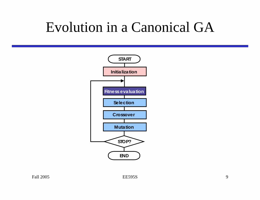
Evolution in a Canonical GA

START

Initialization

Crossover

Mutation

Fitness evaluation

END

STOP?

Selection

Fall 2005 EE595S 10

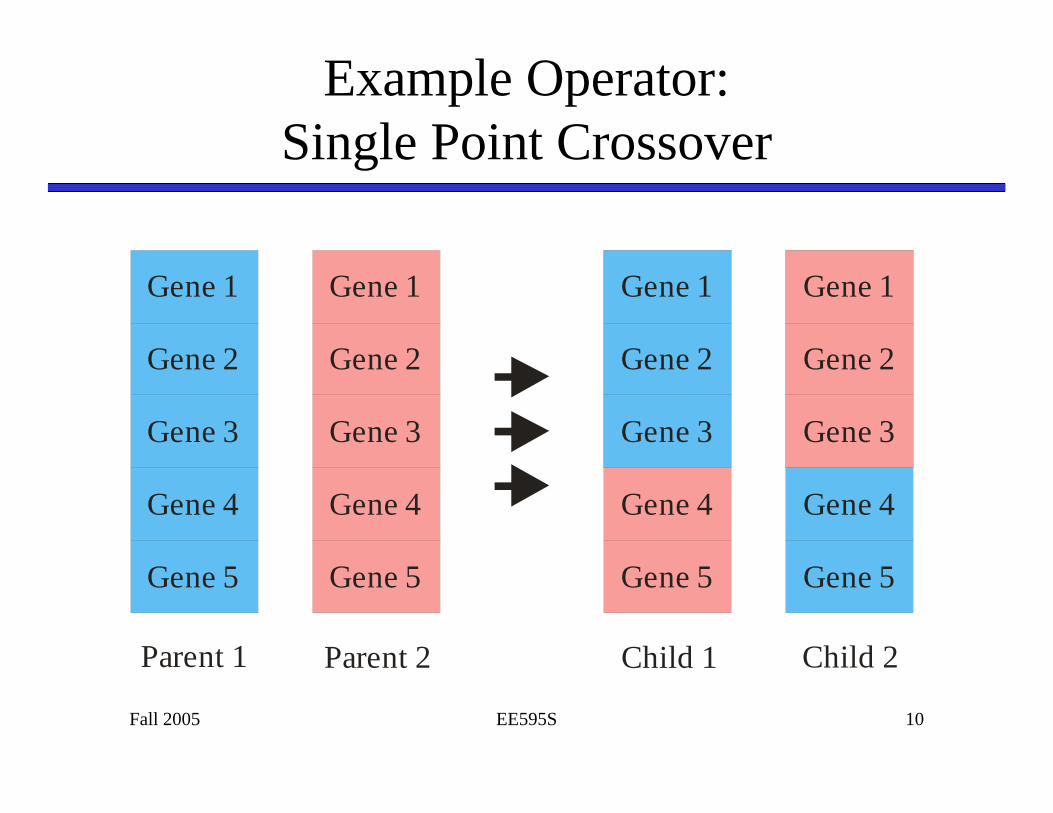
Example Operator:Single Point Crossover

Gene 1

Gene 2

Gene 3

Gene 4

Gene 5

Gene 1

Gene 2

Gene 3

Gene 4

Gene 5

Gene 1

Gene 2

Gene 3

Gene 4

Gene 5

Parent 1

Gene 1

Gene 2

Gene 3

Gene 4

Gene 5

Parent 2 Child 1 Child 2

Fall 2005 EE595S 11

Example Operator:Mutation

Original chromosome 0 1 0 0 0 1 1 0 1 1

Mutated chromosome 0 1 0 0 1 1 1 0 1 1

Mutation point

Fall 2005 EE595S 12

A Gene As A Parameter: Non-Encoded Genetic Algorithms

• Each Gene Has A Range (Minimum Value, Maximum Value)

• Each Gene Has A Type (Mapping)IntegerLinearly Mapped Real NumberLogarithmically Mapped Real Number

• Each Gene is Located on One of a Number of Chromosomes

• Chromosomes Are Haploid

Fall 2005 EE595S 13

Genetic Optimization System Engineering Tool (GOSET)

• Matlab based toolbox• Usable with minimum knowledge• Allows, if desired, high degree of algorithm

control

Fall 2005 EE595S 14

An Individual in GOSET

• A Collection of Genes on Chromosomes

• Fitness (Measures of Goodness)

• Region

Gene 1

Gene 2

Gene 3

Gene 4

Gene 5

Gene 6

Gene 7

Gene 8

Gene 9

Gene 10

Gene 11

Gene 12

Chromosome 1

Chromosome 2

Chromosome 3[ ]TNfff 21=f

Fall 2005 EE595S 15

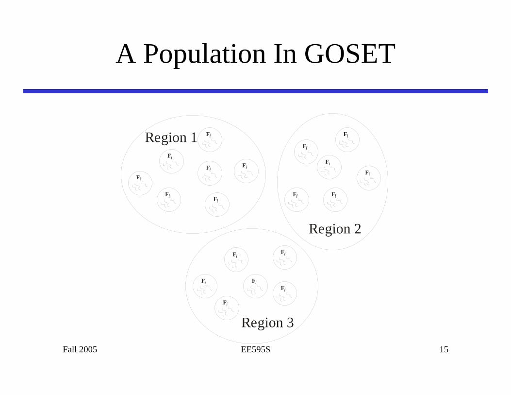
A Population In GOSET

iF

iFiF iF

iF

iFiF

Region 1

iF

iF

iF

iF

iF

iF

Region 2

iF iFiF

iF iF

iF

Region 3

Fall 2005 EE595S 16

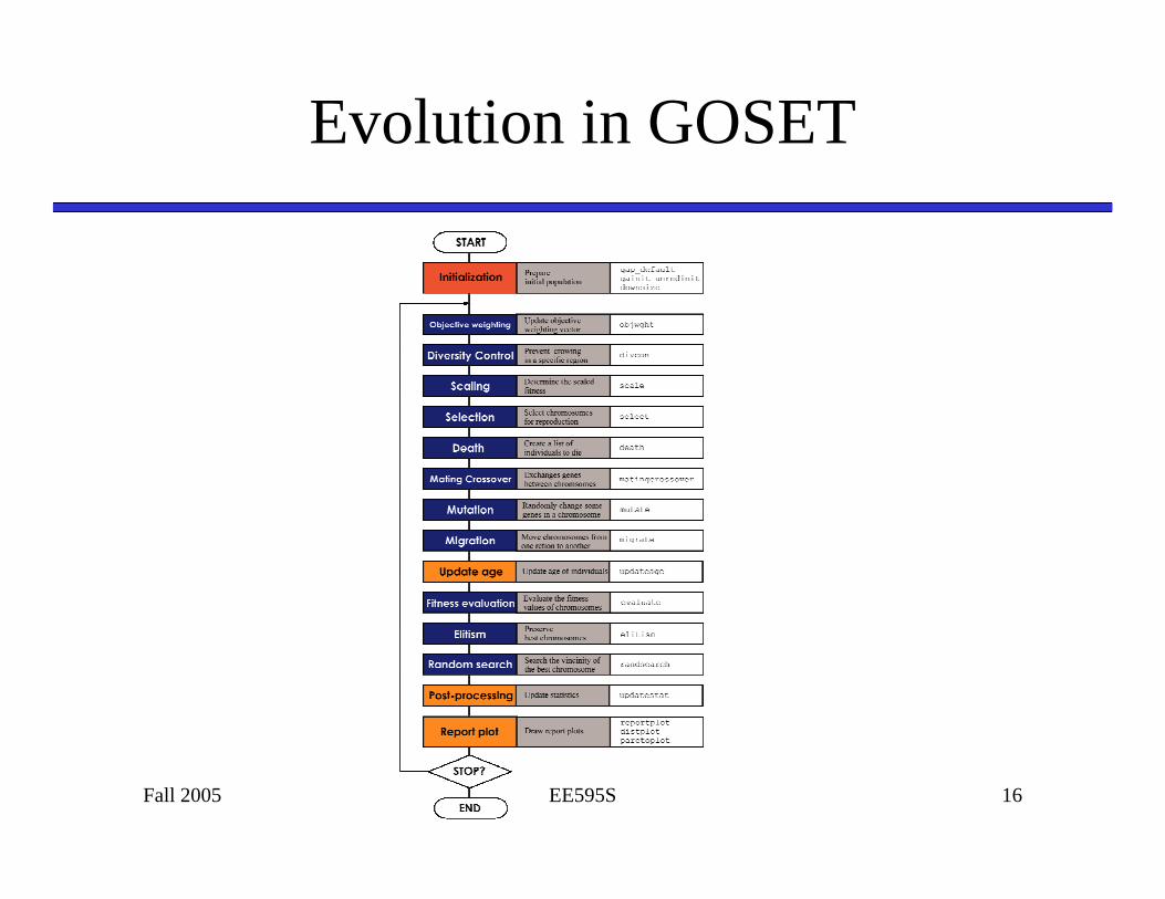
Evolution in GOSET

Fall 2005 EE595S 17

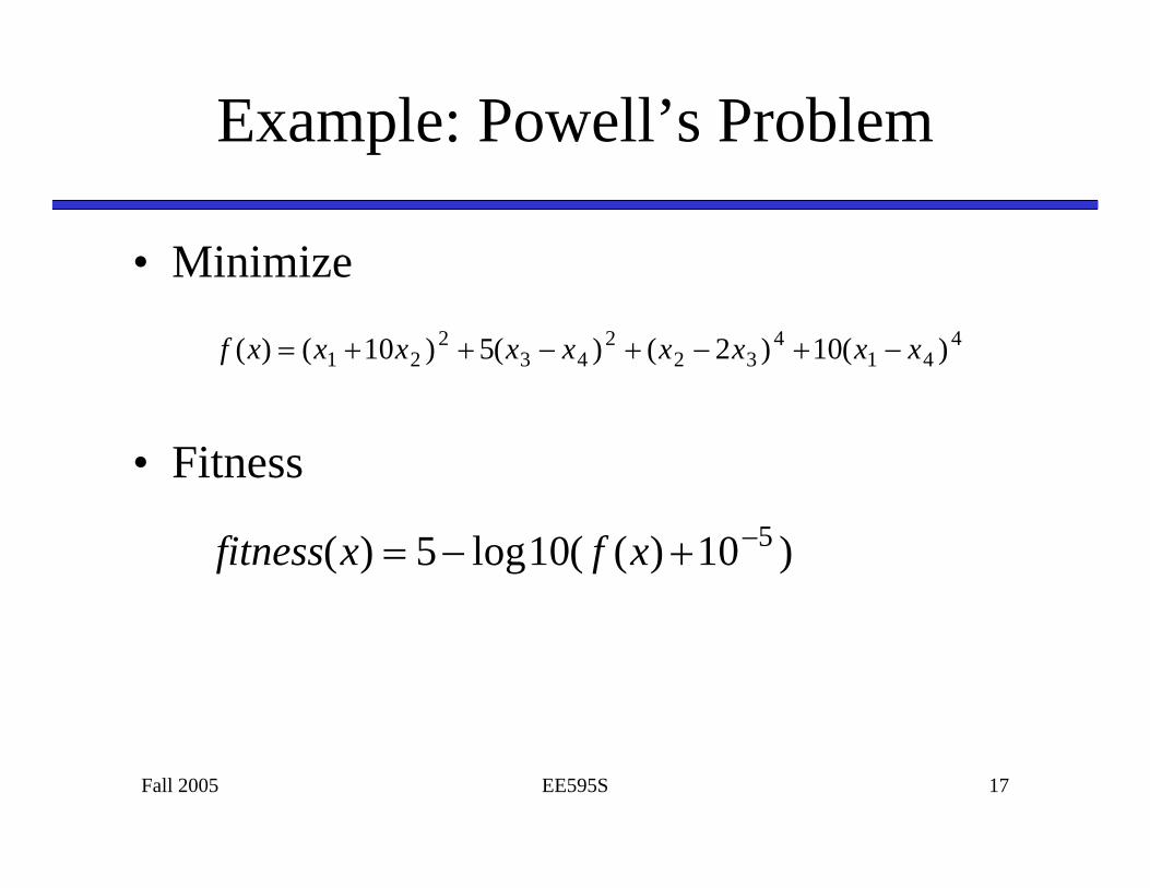
Example: Powell’s Problem

• Minimize

• Fitness

441

432

243

221 )(10)2()(5)10()( xxxxxxxxxf −+−+−++=

)10)((10log5)( 5−+−= xfxfitness

Fall 2005 EE595S 18

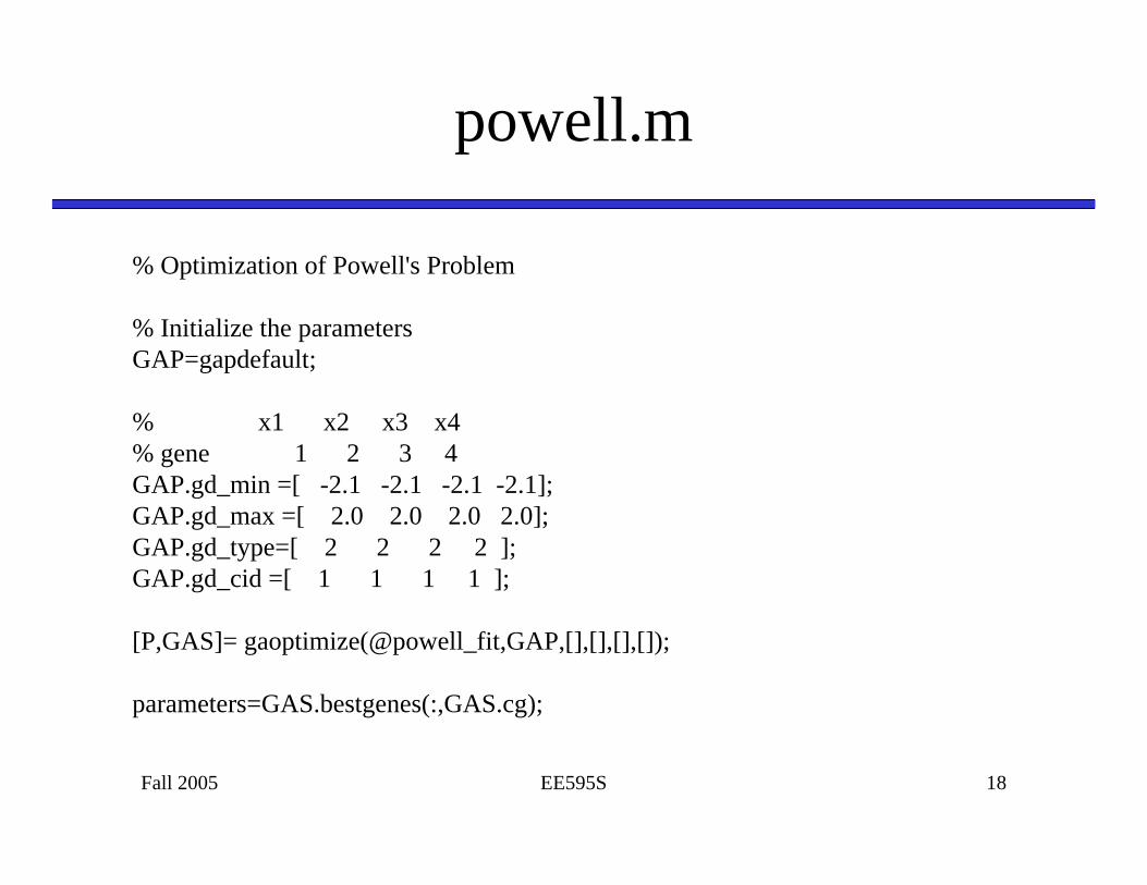
powell.m

% Optimization of Powell's Problem

% Initialize the parametersGAP=gapdefault;

% x1 x2 x3 x4 % gene 1 2 3 4GAP.gd_min =[ -2.1 -2.1 -2.1 -2.1];GAP.gd_max =[ 2.0 2.0 2.0 2.0];GAP.gd_type=[ 2 2 2 2 ];GAP.gd_cid =[ 1 1 1 1 ];

[P,GAS]= gaoptimize(@powell_fit,GAP,[],[],[],[]);

parameters=GAS.bestgenes(:,GAS.cg);

Fall 2005 EE595S 19

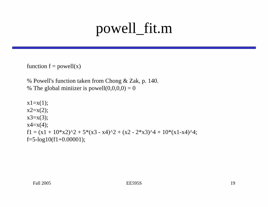
powell_fit.m

function f = powell(x)

% Powell's function taken from Chong & Zak, p. 140.% The global miniizer is powell(0,0,0,0) = 0

x1=x(1);x2=x(2);x3=x(3);x4=x(4);f1 = (x1 + 10*x2)^2 + 5*(x3 - x4)^2 + (x2 - 2*x3)^4 + 10*(x1-x4)^4;f=5-log10(f1+0.00001);

Fall 2005 EE595S 20

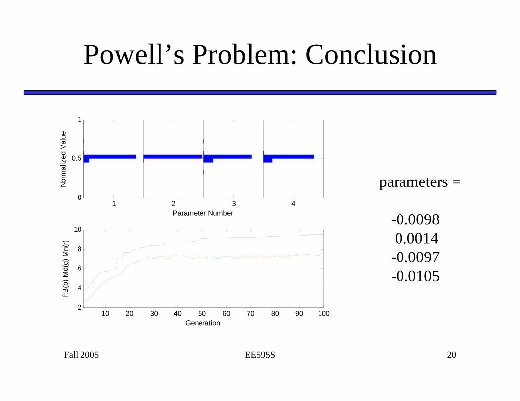
Powell’s Problem: Conclusion

1 2 3 40

0.5

1

Parameter Number

Nor

mal

ized

Val

ue

10 20 30 40 50 60 70 80 90 1002

4

6

8

10

f:B(b

) Md(

g) M

n(r)

Generation

parameters =

-0.00980.0014-0.0097-0.0105

Fall 2005 EE595S 21

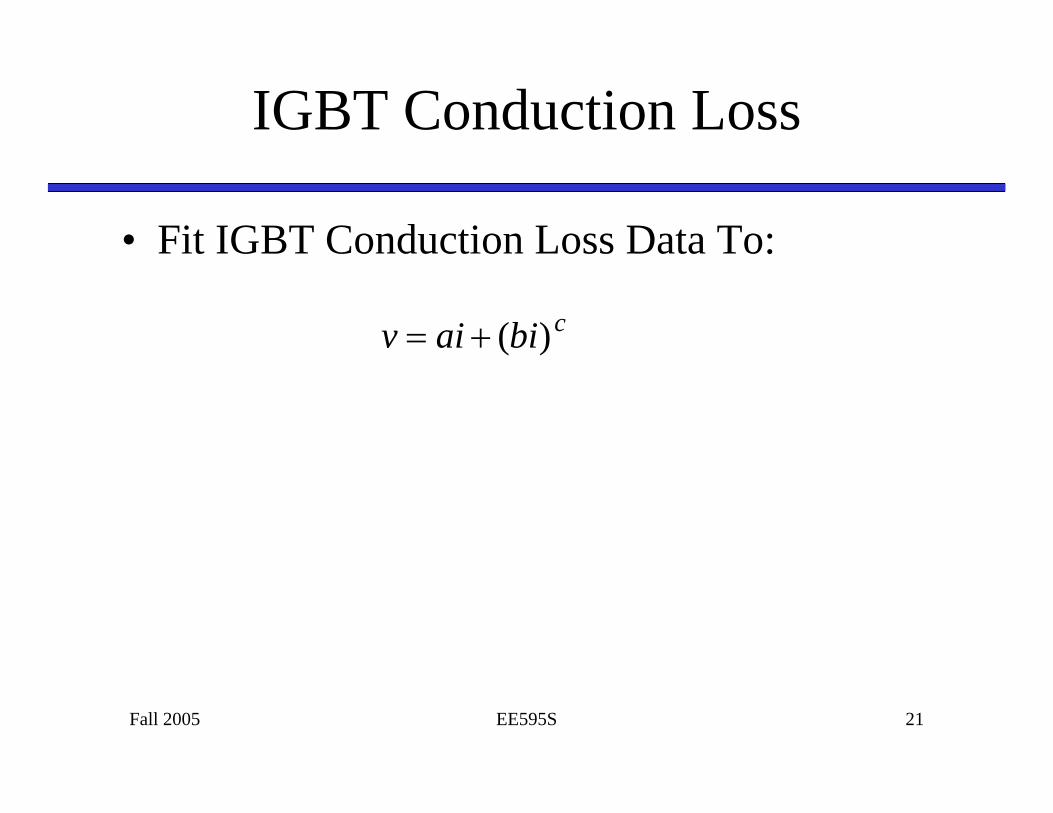
IGBT Conduction Loss

• Fit IGBT Conduction Loss Data To:

cbiaiv )(+=

Fall 2005 EE595S 22

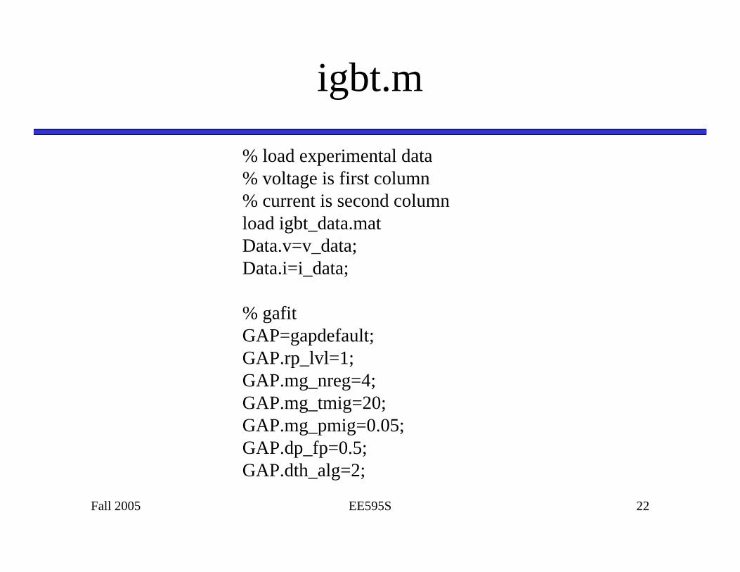
igbt.m

% load experimental data% voltage is first column% current is second columnload igbt_data.matData.v=v_data;Data.i=i_data;

% gafitGAP=gapdefault;GAP.rp_lvl=1;GAP.mg_nreg=4; GAP.mg_tmig=20; GAP.mg_pmig=0.05;GAP.dp_fp=0.5;GAP.dth_alg=2;

Fall 2005 EE595S 23

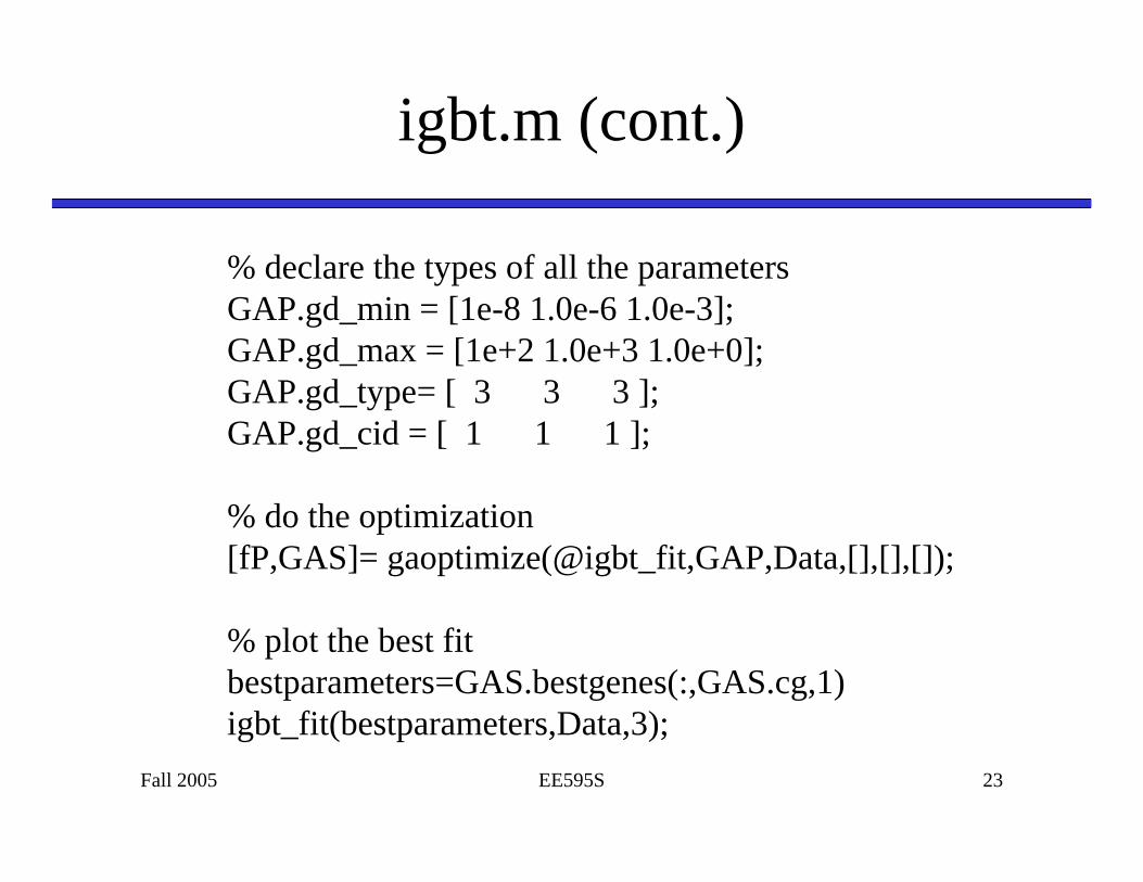
igbt.m (cont.)

% declare the types of all the parametersGAP.gd_min = [1e-8 1.0e-6 1.0e-3];GAP.gd_max = [1e+2 1.0e+3 1.0e+0];GAP.gd_type= [ 3 3 3 ];GAP.gd_cid = [ 1 1 1 ];

% do the optimization[fP,GAS]= gaoptimize(@igbt_fit,GAP,Data,[],[],[]);

% plot the best fitbestparameters=GAS.bestgenes(:,GAS.cg,1)igbt_fit(bestparameters,Data,3);

Fall 2005 EE595S 24

igbt_fit

% this rountine returns the fitness of the IGBT conduction% loss parameters based on the mean percentage errorfunction fitness = IGBTfitness(parameters,data,fignum)

% assign genes to parametersa=parameters(1);b=parameters(2);c=parameters(3);

vpred=a*data.i+(b*data.i).^c;error=abs(1-vpred./data.v);fitness=1.0/(1.0e-6+mean(error));

Fall 2005 EE595S 25

igbt_fit (cont)

if nargin>2

fitness

figure(fignum);Npoints=200;ip=linspace(0,max(data.i),Npoints);vp=a*ip+(b*ip).^c;plot(data.i,data.v,'bx',ip,vp,'r')title('Voltage Versus Currrent');xlabel('Current, A');ylabel('Voltage, V');legend({'Measured','Fit'});

figure(fignum+1);Npoints=200;plot(data.i,data.v.*data.i,'bx',ip,vp.*ip,'r')title('Power Versus Currrent');xlabel('Current, A');ylabel('Power, V');legend({'Measured','Fit'});

end

Fall 2005 EE595S 26

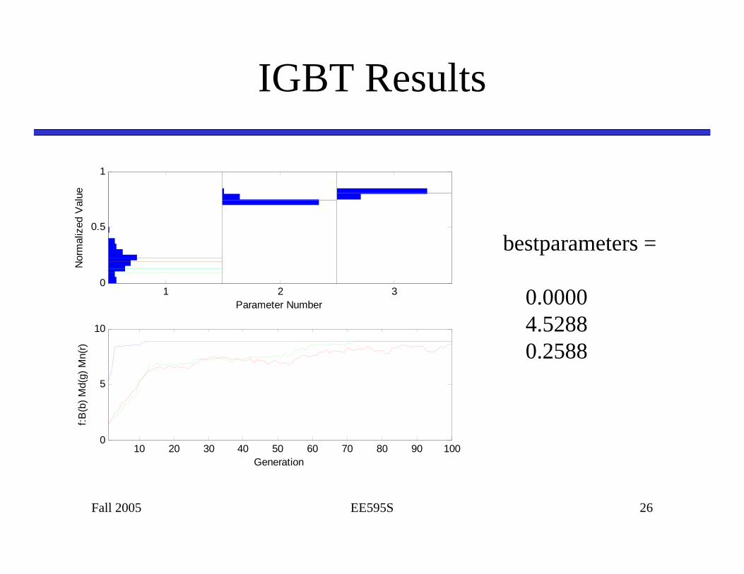
IGBT Results

1 2 30

0.5

1

Parameter Number

Nor

mal

ized

Val

ue

10 20 30 40 50 60 70 80 90 1000

5

10

f:B(b

) Md(

g) M

n(r)

Generation

bestparameters =

0.00004.52880.2588

Fall 2005 EE595S 27

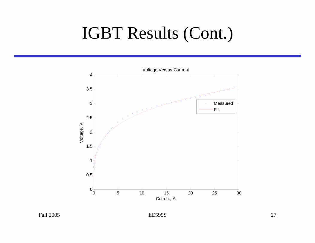
IGBT Results (Cont.)

0 5 10 15 20 25 300

0.5

1

1.5

2

2.5

3

3.5

4Voltage Versus Currrent

Current, A

Vol

tage

, V

MeasuredFit

Fall 2005 EE595S 28

IGBT Results (Cont.)

0 5 10 15 20 25 300

20

40

60

80

100

120Power Versus Currrent

Current, A

Pow

er, V

MeasuredFit

Fall 2005 EE595S 29

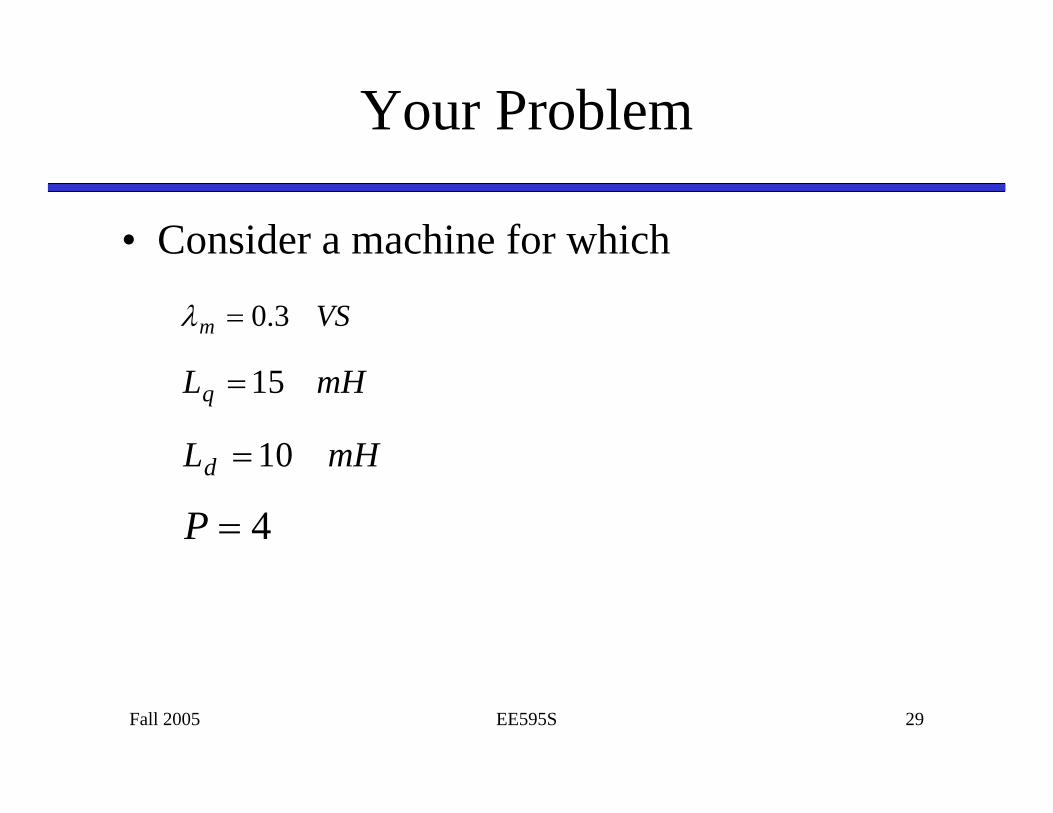
Your Problem

• Consider a machine for which

VSm 3.0=λ

mHLq 15=

mHLd 10=

4=P

Fall 2005 EE595S 30

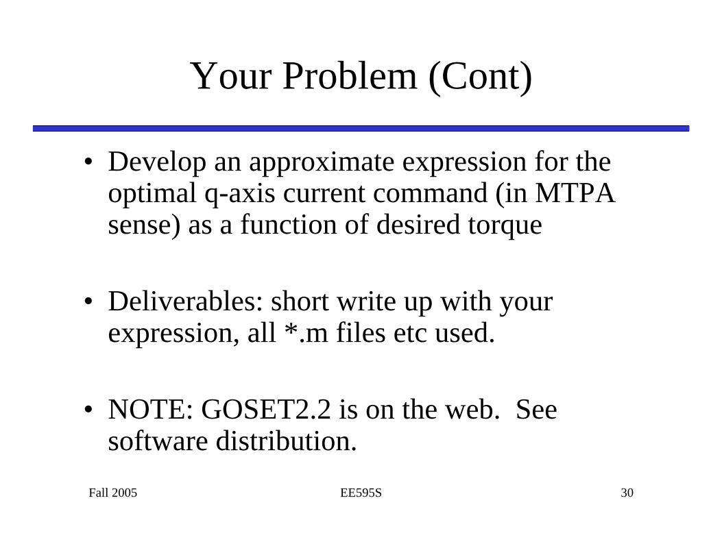
Your Problem (Cont)

• Develop an approximate expression for the optimal q-axis current command (in MTPA sense) as a function of desired torque

• Deliverables: short write up with your expression, all *.m files etc used.

• NOTE: GOSET2.2 is on the web. See software distribution.

Fall 2005 EE595S 31

Comments on Approach