A Brief Tour of SAS - Personal Web Server

1

A Brief Tour of SAS

SAS is one of the most versatile and comprehensive statistical software packages available

today, with data management, analysis, and graphical capabilities. It is great at working with

large databases. SAS has many idiosyncracies and carry-overs from its initial development in a

mainframe environment. This document will introduce some of the key concepts for working

with data using SAS software.

The SAS Desktop

When you open SAS, you will see the SAS desktop with three main windows:

1. The Editor window

This is the window where you create, edit, and submit SAS command files. The default editor is

the Enhanced Editor, which has a system of color coding to make it easier to edit and trouble-

shoot command files.

2. The Log window

This is the window where SAS will echo all of your commands, along with any notes (shown in

blue), error messages (shown in red), and warnings (shown in green). The log window is

cumulative throughout your session and helps to locate any possible problems with a SAS

program.

3. The Explorer window

Among other things, this window shows the libraries that you have defined. SAS libraries are

folders that can contain SAS datasets and catalogs. When you start SAS, you will automatically

have the libraries Work, Sasuser, and Sashelp defined, plus Maps, if you have SAS/Maps on

your system. You can define other libraries where you wish to store and access datasets, as we

will see later. If you accidentally close this window, go to View > Contents Only to reopen it.

2

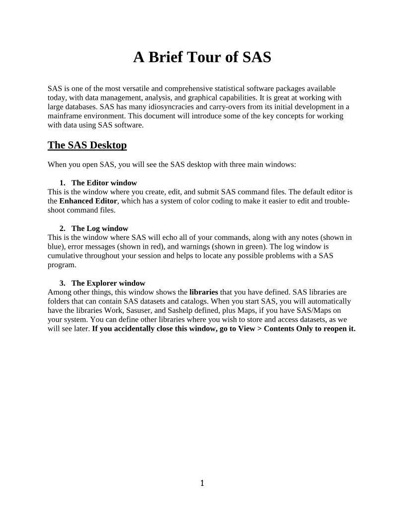
Additional Windows

1. The Output window

This window will be behind other windows until you generate some output. The text in this

window can be copied and pasted to a word processing program, but it cannot be edited or

modified.

2. The SAS/Graph window

This window will not open until you generate graphs using procedures such as Proc Gplot or

Proc Univariate.

You can navigate among the SAS windows in this environment. Different menu options are

available depending on which window you are using.

Set the current directory

To do this, double-click on the directory location at the bottom of the SAS workspace window.

You will be able to browse to the folder to use. This folder will be the default location where

SAS command files and raw data files will be read from/written to.

3

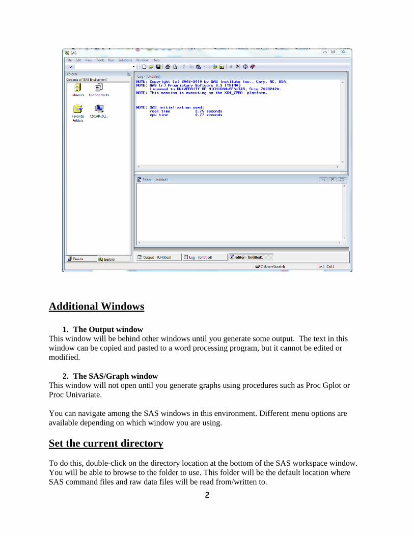
Browse to the folder to use for the current folder, and then click on OK.

Double-click here to change the current directory.

4

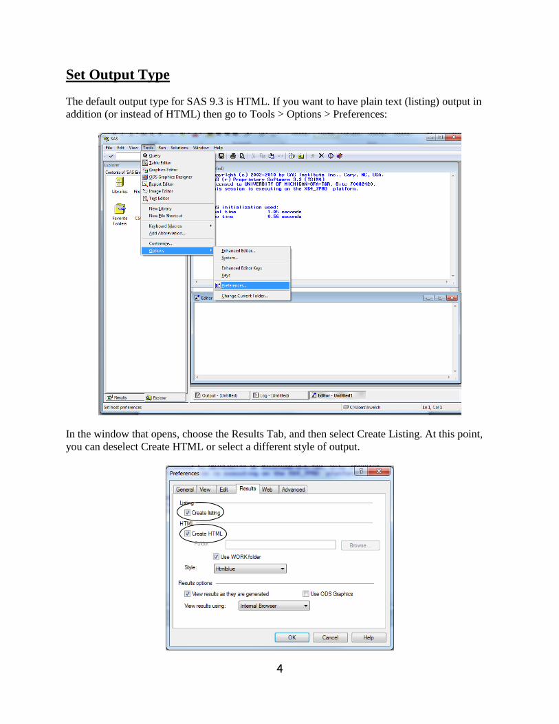
Set Output Type

The default output type for SAS 9.3 is HTML. If you want to have plain text (listing) output in

addition (or instead of HTML) then go to Tools > Options > Preferences:

In the window that opens, choose the Results Tab, and then select Create Listing. At this point,

you can deselect Create HTML or select a different style of output.

5

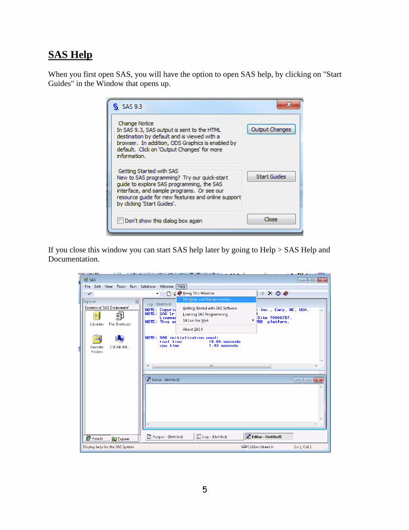
SAS Help

When you first open SAS, you will have the option to open SAS help, by clicking on "Start

Guides" in the Window that opens up.

If you close this window you can start SAS help later by going to Help > SAS Help and

Documentation.

6

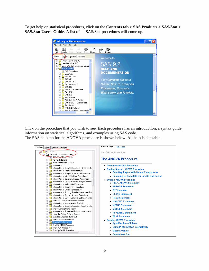
To get help on statistical procedures, click on the Contents tab > SAS Products > SAS/Stat >

SAS/Stat User's Guide. A list of all SAS/Stat procedures will come up.

Click on the procedure that you wish to see. Each procedure has an introduction, a syntax guide,

information on statistical algorithms, and examples using SAS code.

The SAS help tab for the ANOVA procedure is shown below. All help is clickable.

7

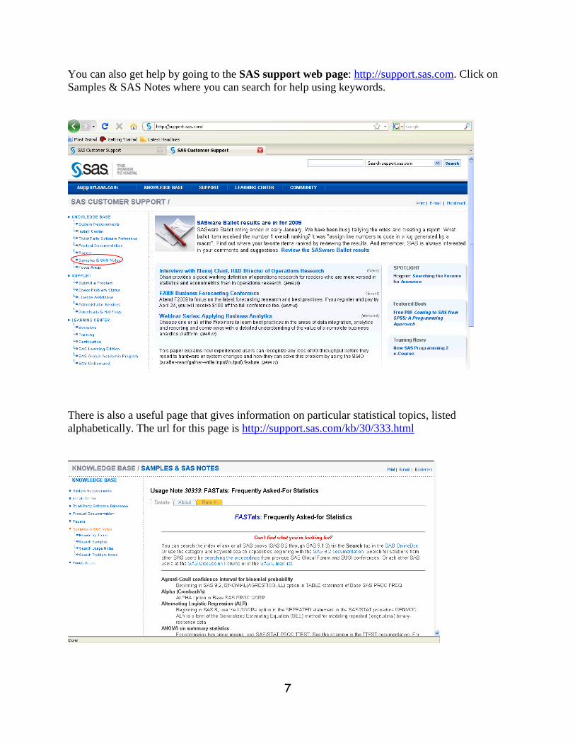
You can also get help by going to the SAS support web page: http://support.sas.com. Click on

Samples & SAS Notes where you can search for help using keywords.

There is also a useful page that gives information on particular statistical topics, listed

alphabetically. The url for this page is http://support.sas.com/kb/30/333.html

http://support.sas.com/

http://support.sas.com/kb/30/333.html

8

Getting Datasets into SAS

Before you can get started with SAS, you will first need either to read in some raw data, or open

an existing SAS dataset.

Reading in raw data in plain text free format

Here is an excerpt of a raw data file that has each value separated by blanks (free format). The

name of the raw data file is class.dat. Missing values are indicated by a period (.), with a blank

between periods for contiguous missing values.

Warren F 29 68 139

Kalbfleisch F 35 64 120

Pierce M . . 112

Walker F 22 56 133

Rogers M 45 68 145

Baldwin M 47 72 128

Mims F 48 67 152

Lambini F 36 . 120

Gossert M . 73 139

The SAS data step to read this type of raw data is shown below. The data statement names the

data set to be created, and the infile statement indicates the raw data file to be read. The input

statement lists the variables to be read in the order in which they appear in the raw data file. No

variables can be skipped at the beginning of the variable list, but you may stop reading variables

before reaching the end of the list.

data class;

infile "class.dat";

input lname $ sex $ age height sbp;

run;

Note that character variables are followed by a $. Without a $ after a variable name, SAS

assumes that the variable is numeric (the default).

Check the SAS log to be sure the dataset was correctly created.

1 data class;

2 infile "class.dat";

3 input lname $ sex $ age height sbp;

4 run;

NOTE: The infile "class.dat" is:

Filename=C:\Users\kwelch\Desktop\b512\class.dat,

RECFM=V,LRECL=256,File Size (bytes)=286,

Last Modified=05Oct1998:00:44:32,

NOTE: 14 records were read from the infile "class.dat".

The minimum record length was 16.

The maximum record length was 23.

NOTE: The data set WORK.CLASS has 14 observations and 5 variables.

NOTE: DATA statement used (Total process time):

2 data class;

9

3 infile "class.dat";

4 input lname $ sex $ age height sbp;

5 run;

NOTE: The infile "class.dat" is:

Filename=C:\Users\kwelch\Desktop\b512\class.dat,


Last Modified=04Oct1998:23:44:32,

Create Time=10Jan2011:12:56:56

NOTE: 14 records were read from the infile "class.dat".



NOTE: The data set WORK.CLASS has 14 observations and 5 variables.

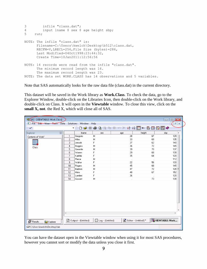
Note that SAS automatically looks for the raw data file (class.dat) in the current directory.

This dataset will be saved in the Work library as Work.Class. To check the data, go to the

Explorer Window, double-click on the Libraries Icon, then double-click on the Work library, and

double-click on Class. It will open in the Viewtable window. To close this view, click on the

small X, not. the Red X, which will close all of SAS.

You can have the dataset open in the Viewtable window when using it for most SAS procedures,

however you cannot sort or modify the data unless you close it first.

10

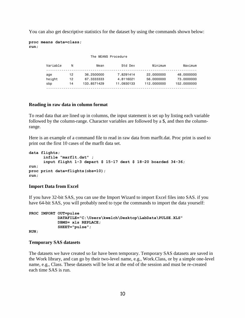
You can also get descriptive statistics for the dataset by using the commands shown below:

proc means data=class;

run;

The MEANS Procedure

Variable N Mean Std Dev Minimum Maximum

------------------------------------------------------------------------------

age 12 36.2500000 7.8291414 22.0000000 48.0000000

height 12 67.3333333 4.8116021 56.0000000 73.0000000

sbp 14 133.8571429 11.0930133 112.0000000 152.0000000

------------------------------------------------------------------------------

Reading in raw data in column format

To read data that are lined up in columns, the input statement is set up by listing each variable

followed by the column-range. Character variables are followed by a $, and then the column-

range.

Here is an example of a command file to read in raw data from marflt.dat. Proc print is used to

print out the first 10 cases of the marflt data set.

data flights;

infile "marflt.dat" ;

input flight 1-3 depart $ 15-17 dest $ 18-20 boarded 34-36;

run;

proc print data=flights(obs=10);

run;

Import Data from Excel

If you have 32-bit SAS, you can use the Import Wizard to import Excel files into SAS. if you

have 64-bit SAS, you will probably need to type the commands to import the data yourself:

PROC IMPORT OUT=pulse

DATAFILE="C:\Users\kwelch\Desktop\LabData\PULSE.XLS"

DBMS= xls REPLACE;

SHEET="pulse";

RUN;

Temporary SAS datasets

The datasets we have created so far have been temporary. Temporary SAS datasets are saved in

the Work library, and can go by their two-level name, e.g., Work.Class, or by a simple one-level

name, e.g., Class. These datasets will be lost at the end of the session and must be re-created

each time SAS is run.

11

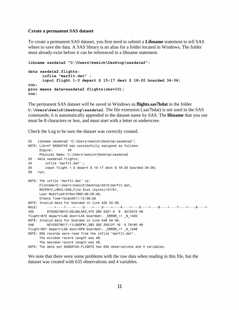
Create a permanent SAS dataset

To create a permanent SAS dataset, you first need to submit a Libname statement to tell SAS

where to save the data. A SAS library is an alias for a folder located in Windows. The folder

must already exist before it can be referenced in a libname statement.

libname sasdata2 "C:\Users\kwelch\Desktop\sasdata2";

data sasdata2.flights;

infile "marflt.dat" ;

input flight 1-3 depart $ 15-17 dest $ 18-20 boarded 34-36;

run;

proc means data=sasdata2.flights(obs=10);

run;

The permanent SAS dataset will be saved in Windows as flights.sas7bdat in the folder

C:\Users\kwelch\Desktop\sasdata2. The file extension (.sas7bdat) is not used in the SAS

commands; it is automatically appended to the dataset name by SAS. The libname that you use

must be 8 characters or less, and must start with a letter or underscore.

Check the Log to be sure the dataset was correctly created.

22 libname sasdata2 "C:\Users\kwelch\Desktop\sasdata2";

NOTE: Libref SASDATA2 was successfully assigned as follows:

Engine: V9

Physical Name: C:\Users\kwelch\Desktop\sasdata2

23 data sasdata2.flights;

24 infile "marflt.dat" ;

25 input flight 1-3 depart $ 15-17 dest $ 18-20 boarded 34-36;

26 run;

NOTE: The infile "marflt.dat" is:

Filename=C:\Users\kwelch\Desktop\b512\marflt.dat,


Last Modified=21Dec1993:06:26:46,

Create Time=10Jan2011:12:56:56 NOTE: Invalid data for boarded in line 420 34-36.

RULE: ----+----1----+----2----+----3----+----4----+----5----+----6----+----7----+----8----+-

420 87203219013:02LGALAX2,475 283 5321-3 9 0210210 48

flight=872 depart=LGA dest=LAX boarded=. _ERROR_=1 _N_=420

NOTE: Invalid data for boarded in line 548 34-36.

548 92103279017:11LGADFW1,383 282 25012ª 16 5 79180 48

flight=921 depart=LGA dest=DFW boarded=. _ERROR_=1 _N_=548

NOTE: 635 records were read from the infile "marflt.dat".



NOTE: The data set SASDATA2.FLIGHTS has 635 observations and 4 variables.

We note that there were some problems with the raw data when reading in this file, but the

dataset was created with 635 observations and 4 variables.

12

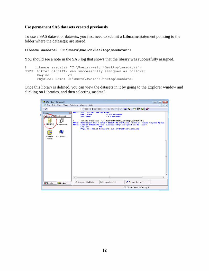
Use permanent SAS datasets created previously

To use a SAS dataset or datasets, you first need to submit a Libname statement pointing to the

folder where the dataset(s) are stored.


You should see a note in the SAS log that shows that the library was successfully assigned.

1 libname sasdata2 "C:\Users\kwelch\Desktop\sasdata2";

NOTE: Libref SASDATA2 was successfully assigned as follows:

Engine: V9

Physical Name: C:\Users\kwelch\Desktop\sasdata2

Once this library is defined, you can view the datasets in it by going to the Explorer window and

clicking on Libraries, and then selecting sasdata2.

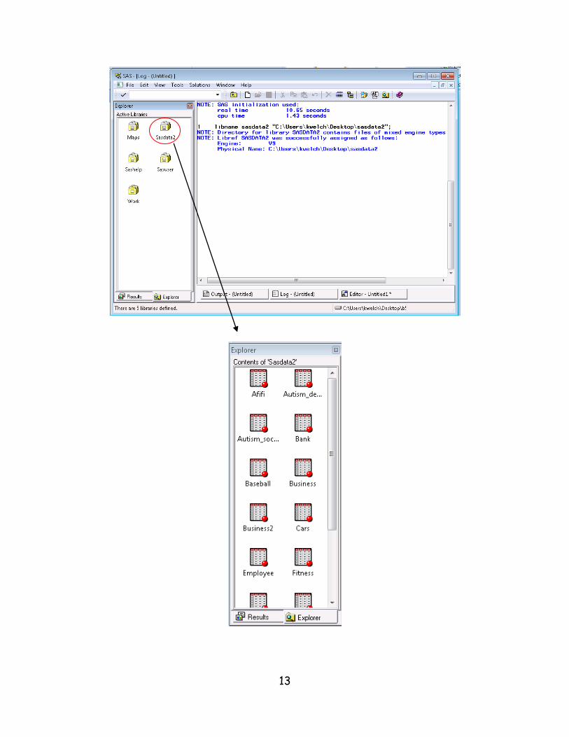
13

14

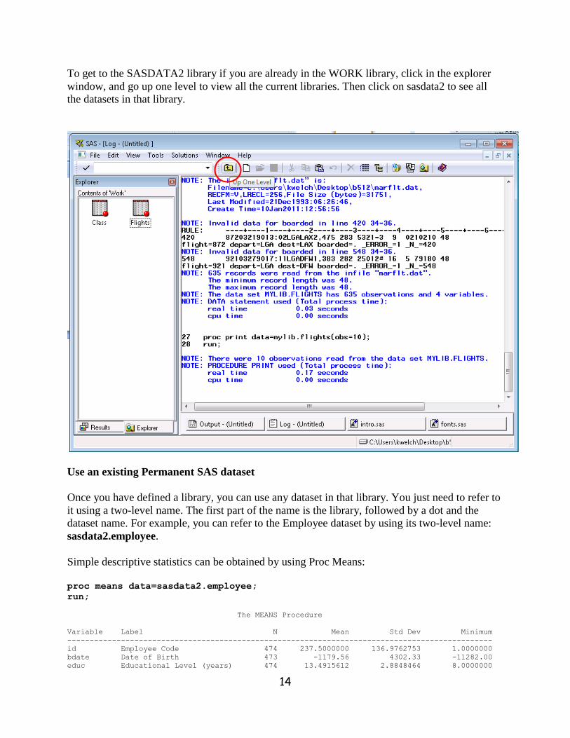
To get to the SASDATA2 library if you are already in the WORK library, click in the explorer

window, and go up one level to view all the current libraries. Then click on sasdata2 to see all

the datasets in that library.

Use an existing Permanent SAS dataset

Once you have defined a library, you can use any dataset in that library. You just need to refer to

it using a two-level name. The first part of the name is the library, followed by a dot and the

dataset name. For example, you can refer to the Employee dataset by using its two-level name:

sasdata2.employee.

Simple descriptive statistics can be obtained by using Proc Means:

proc means data=sasdata2.employee;

run;

The MEANS Procedure

Variable Label N Mean Std Dev Minimum

-----------------------------------------------------------------------------------------------

id Employee Code 474 237.5000000 136.9762753 1.0000000

bdate Date of Birth 473 -1179.56 4302.33 -11282.00

educ Educational Level (years) 474 13.4915612 2.8848464 8.0000000

15

jobcat Employment Category 474 1.4113924 0.7732014 1.0000000

salary Current Salary 474 34419.57 17075.66 15750.00

salbegin Beginning Salary 474 17016.09 7870.64 9000.00

jobtime Months since Hire 474 81.1097046 10.0609449 63.0000000

prevexp Previous Experience (months) 474 95.8607595 104.5862361 0

minority Minority Classification 474 0.2194093 0.4142836 0

-----------------------------------------------------------------------------------------------

Variable Label Maximum

--------------------------------------------------------

id Employee Code 474.0000000

bdate Date of Birth 4058.00

educ Educational Level (years) 21.0000000

jobcat Employment Category 3.0000000

salary Current Salary 135000.00

salbegin Beginning Salary 79980.00

jobtime Months since Hire 98.0000000

prevexp Previous Experience (months) 476.0000000

minority Minority Classification 1.0000000

--------------------------------------------------------

Selecting cases for analysis

You can select cases for an analysis using the Where statement in your commands:

proc print data=sasdata2.employee;

where jobcat=1;

run;

The SAS System

Obs id gender bdate educ jobcat salary salbegin jobtime prevexp minority

2 2 m -588 16 1 40200 18750 98 36 0

3 3 f -11116 12 1 21450 12000 98 381 0

4 4 f -4644 8 1 21900 13200 98 190 0

5 5 m -1787 15 1 45000 21000 98 138 0

6 6 m -497 15 1 32100 13500 98 67 0

7 7 m -1345 15 1 36000 18750 98 114 0

8 8 f 2317 12 1 21900 9750 98 0 0

9 9 f -5091 15 1 27900 12750 98 115 0

10 10 f -5070 12 1 24000 13500 98 244 0

11 11 f -3615 16 1 30300 16500 98 143 0

12 12 m 2202 8 1 28350 12000 98 26 1

13 13 m 198 15 1 27750 14250 98 34 1

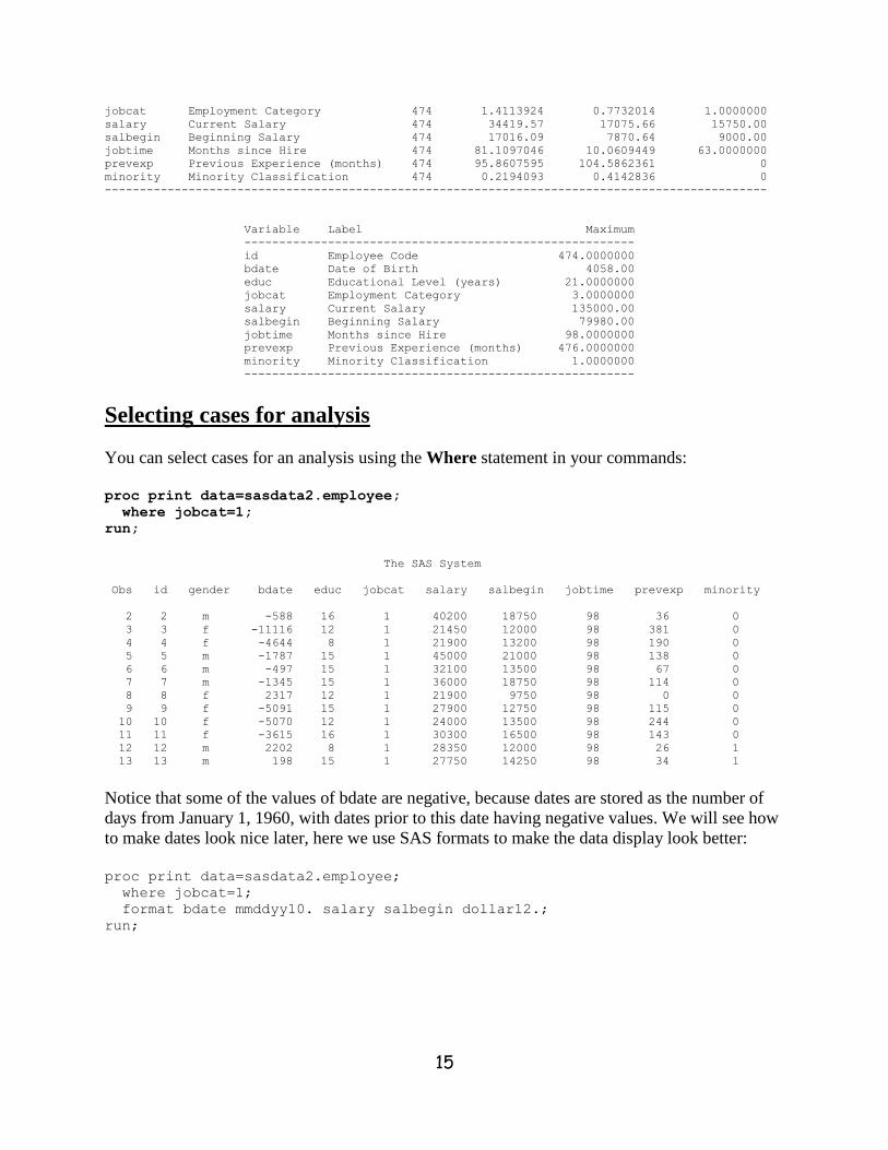
Notice that some of the values of bdate are negative, because dates are stored as the number of

days from January 1, 1960, with dates prior to this date having negative values. We will see how

to make dates look nice later, here we use SAS formats to make the data display look better:

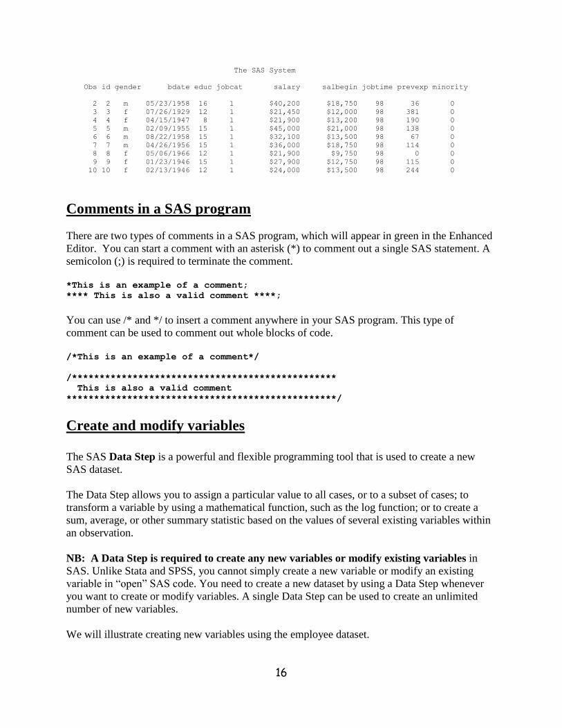
proc print data=sasdata2.employee;

where jobcat=1;

format bdate mmddyy10. salary salbegin dollar12.;

run;

16

The SAS System

Obs id gender bdate educ jobcat salary salbegin jobtime prevexp minority

2 2 m 05/23/1958 16 1 $40,200 $18,750 98 36 0

3 3 f 07/26/1929 12 1 $21,450 $12,000 98 381 0

4 4 f 04/15/1947 8 1 $21,900 $13,200 98 190 0

5 5 m 02/09/1955 15 1 $45,000 $21,000 98 138 0

6 6 m 08/22/1958 15 1 $32,100 $13,500 98 67 0

7 7 m 04/26/1956 15 1 $36,000 $18,750 98 114 0

8 8 f 05/06/1966 12 1 $21,900 $9,750 98 0 0

9 9 f 01/23/1946 15 1 $27,900 $12,750 98 115 0

10 10 f 02/13/1946 12 1 $24,000 $13,500 98 244 0

Comments in a SAS program

There are two types of comments in a SAS program, which will appear in green in the Enhanced

Editor. You can start a comment with an asterisk (*) to comment out a single SAS statement. A

semicolon (;) is required to terminate the comment.

*This is an example of a comment;

**** This is also a valid comment ****;

You can use /* and */ to insert a comment anywhere in your SAS program. This type of

comment can be used to comment out whole blocks of code.

/*This is an example of a comment*/

/************************************************

This is also a valid comment

*************************************************/

Create and modify variables

The SAS Data Step is a powerful and flexible programming tool that is used to create a new

SAS dataset.

The Data Step allows you to assign a particular value to all cases, or to a subset of cases; to

transform a variable by using a mathematical function, such as the log function; or to create a

sum, average, or other summary statistic based on the values of several existing variables within

an observation.

NB: A Data Step is required to create any new variables or modify existing variables in

SAS. Unlike Stata and SPSS, you cannot simply create a new variable or modify an existing

variable in “open” SAS code. You need to create a new dataset by using a Data Step whenever

you want to create or modify variables. A single Data Step can be used to create an unlimited

number of new variables.

We will illustrate creating new variables using the employee dataset.

17

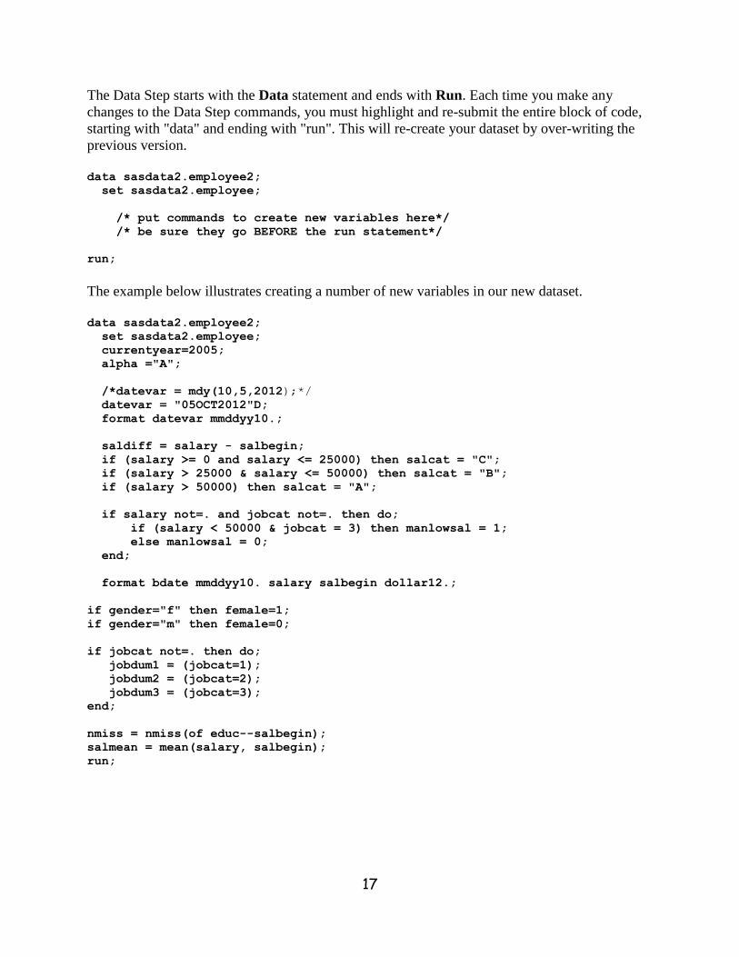
The Data Step starts with the Data statement and ends with Run. Each time you make any

changes to the Data Step commands, you must highlight and re-submit the entire block of code,

starting with "data" and ending with "run". This will re-create your dataset by over-writing the

previous version.

data sasdata2.employee2;

set sasdata2.employee;

/* put commands to create new variables here*/

/* be sure they go BEFORE the run statement*/

run;

The example below illustrates creating a number of new variables in our new dataset.

data sasdata2.employee2;

set sasdata2.employee;

currentyear=2005;

alpha ="A";

/*datevar = mdy(10,5,2012);*/

datevar = "05OCT2012"D;

format datevar mmddyy10.;

saldiff = salary - salbegin;

if (salary >= 0 and salary <= 25000) then salcat = "C";

if (salary > 25000 & salary <= 50000) then salcat = "B";

if (salary > 50000) then salcat = "A";

if salary not=. and jobcat not=. then do;

if (salary < 50000 & jobcat = 3) then manlowsal = 1;

else manlowsal = 0;

end;

format bdate mmddyy10. salary salbegin dollar12.;

if gender="f" then female=1;

if gender="m" then female=0;

if jobcat not=. then do;

jobdum1 = (jobcat=1);



end;

nmiss = nmiss(of educ--salbegin);

salmean = mean(salary, salbegin);

run;

18

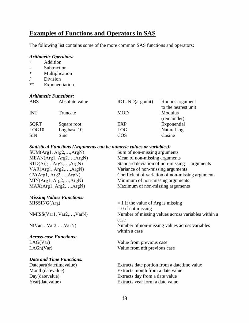
Examples of Functions and Operators in SAS

The following list contains some of the more common SAS functions and operators:

Arithmetic Operators:

+ Addition

- Subtraction

* Multiplication

/ Division

** Exponentiation

Arithmetic Functions:

ABS Absolute value ROUND(arg,unit) Rounds argument

to the nearest unit

INT Truncate MOD Modulus

(remainder)

SQRT Square root EXP Exponential

LOG10 Log base 10 LOG Natural log

SIN Sine COS Cosine

Statistical Functions (Arguments can be numeric values or variables):

SUM(Arg1, Arg2,…,ArgN) Sum of non-missing arguments

MEAN(Arg1, Arg2,…,ArgN) Mean of non-missing arguments

STD(Arg1, Arg2,…,ArgN) Standard deviation of non-missing arguments

VAR(Arg1, Arg2,…,ArgN) Variance of non-missing arguments

CV(Arg1, Arg2,…,ArgN) Coefficient of variation of non-missing arguments

MIN(Arg1, Arg2,…,ArgN) Minimum of non-missing arguments

MAX(Arg1, Arg2,…,ArgN) Maximum of non-missing arguments

Missing Values Functions: MISSING(Arg) = 1 if the value of Arg is missing

= 0 if not missing

NMISS(Var1, Var2,…,VarN) Number of missing values across variables within a

case

N(Var1, Var2,…,VarN) Number of non-missing values across variables

within a case

Across-case Functions: LAG(Var) Value from previous case

LAGn(Var) Value from nth previous case

Date and Time Functions:

Datepart(datetimevalue) Extracts date portion from a datetime value

Month(datevalue) Extracts month from a date value

Day(datevalue) Extracts day from a date value

Year(datevalue) Extracts year form a date value

19

Intck(‘interval’,datestart,dateend) Finds the number of completed intervals between

two dates

Other Functions: RANUNI(Seed) Uniform pseudo-random no. defined on the interval

(0,1)

RANNOR(Seed) Std. Normal pseudo-random no.

PROBNORM(x) Prob. a std. normal is <= x

PROBIT(p) pth

quantile from std. normal dist.

Numeric vs. Character Variables

There are only two types of variable in SAS: numeric and character. Numeric variables are the

default type and are used for numeric and date values.

Character variables can have alpha-numeric values, which may be any combination of letters,

numbers, or other characters. The length of a character variable can be up to 32767 characters.

Values of character variables are case-sensitive. For example, the value “Ann Arbor” is different

than the value “ANN ARBOR”.

Generating Variables Containing Constants

In the example below we create a new numeric variable named “currentyear”, which has a

constant value of 2005 for all observations:

currentyear=2005;

The example below illustrates creating a new character variable named “alpha” which contains

the letter “A” for all observations in the dataset. Note that the value must be enclosed either in

single or double-quotes, because this is a character variable.

alpha ="A";

Dates can be generated in a number of different ways. For example, we can use the mdy function

to create a date value from a month, day, and year value, as shown below:

datevar = mdy(10,5,2012);

Or we can create a date by using a SAS date constant, as shown below:

datevar = "05OCT2012"D;

The D following the quoted date constant tells SAS that this is not a character variable, but a date

value, which is stored as a numeric value.

format datevar mmddyy10.;

20

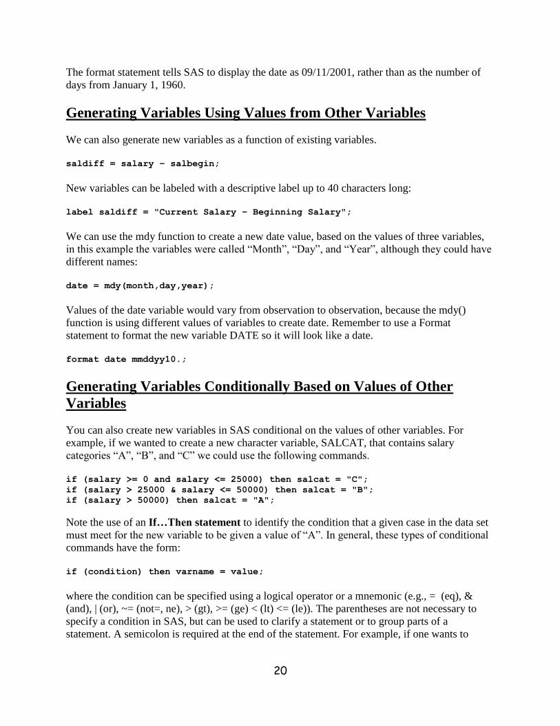
The format statement tells SAS to display the date as 09/11/2001, rather than as the number of

days from January 1, 1960.

Generating Variables Using Values from Other Variables

We can also generate new variables as a function of existing variables.

saldiff = salary – salbegin;

New variables can be labeled with a descriptive label up to 40 characters long:

label saldiff = "Current Salary – Beginning Salary";

We can use the mdy function to create a new date value, based on the values of three variables,

in this example the variables were called “Month”, “Day”, and “Year”, although they could have

different names:

date = mdy(month,day,year);

Values of the date variable would vary from observation to observation, because the mdy()

function is using different values of variables to create date. Remember to use a Format

statement to format the new variable DATE so it will look like a date.

format date mmddyy10.;

Generating Variables Conditionally Based on Values of Other

Variables

You can also create new variables in SAS conditional on the values of other variables. For

example, if we wanted to create a new character variable, SALCAT, that contains salary

categories “A”, “B”, and “C” we could use the following commands.

if (salary >= 0 and salary <= 25000) then salcat = "C";

if (salary > 25000 & salary <= 50000) then salcat = "B";

if (salary > 50000) then salcat = "A";

Note the use of an If…Then statement to identify the condition that a given case in the data set

must meet for the new variable to be given a value of “A”. In general, these types of conditional

commands have the form:

if (condition) then varname = value;

where the condition can be specified using a logical operator or a mnemonic (e.g., = (eq), &

(and), | (or), ~= (not=, ne), > (gt), >= (ge) < (lt) <= (le)). The parentheses are not necessary to

specify a condition in SAS, but can be used to clarify a statement or to group parts of a

statement. A semicolon is required at the end of the statement. For example, if one wants to

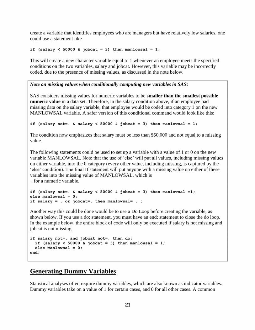
21

create a variable that identifies employees who are managers but have relatively low salaries, one

could use a statement like


This will create a new character variable equal to 1 whenever an employee meets the specified

conditions on the two variables, salary and jobcat. However, this variable may be incorrectly

coded, due to the presence of missing values, as discussed in the note below.

Note on missing values when conditionally computing new variables in SAS:

SAS considers missing values for numeric variables to be smaller than the smallest possible

numeric value in a data set. Therefore, in the salary condition above, if an employee had

missing data on the salary variable, that employee would be coded into category 1 on the new

MANLOWSAL variable. A safer version of this conditional command would look like this:

if (salary not=. & salary < 50000 & jobcat = 3) then manlowsal = 1;

The condition now emphasizes that salary must be less than $50,000 and not equal to a missing

value.

The following statements could be used to set up a variable with a value of 1 or 0 on the new

variable MANLOWSAL. Note that the use of ‘else’ will put all values, including missing values

on either variable, into the 0 category (every other value, including missing, is captured by the

‘else’ condition). The final If statement will put anyone with a missing value on either of these

variables into the missing value of MANLOWSAL, which is

. for a numeric variable.

if (salary not=. & salary < 50000 & jobcat = 3) then manlowsal =1;

else manlowsal = 0;

if salary = . or jobcat=. then manlowsal= . ;

Another way this could be done would be to use a Do Loop before creating the variable, as

shown below. If you use a do; statement, you must have an end; statement to close the do loop.

In the example below, the entire block of code will only be executed if salary is not missing and

jobcat is not missing.

if salary not=. and jobcat not=. then do;


else manlowsal = 0;

end;

Generating Dummy Variables

Statistical analyses often require dummy variables, which are also known as indicator variables.

Dummy variables take on a value of 1 for certain cases, and 0 for all other cases. A common

22

example is the creation of a dummy variable to recode, where the value of 1 might identify

females, and 0 males.

if gender="f" then female=1;

if gender="m" then female=0;

If you have a variable with 3 or more categories, you can create a dummy variable for each

category, and later in a regression analysis, you would usually choose to include one less dummy

variable than there are categories in your model.

if jobcat not=. then do;




end;

Using Statistical Functions

You can also use SAS to determine how many missing values are present in a list of variables

within an observation, as shown in the example below:

nmiss = nmiss(of educ--salbegin);

The double dashes (--) indicate a variable list (with variables given in dataset order). Be sure to

use “of” when using a variable list like this.

The converse operation is to determine the number of non-missing values there are in a list of

variables,

npresent = n(of educ--salbegin);

Another common operation is to calculate the sum or the mean of the values for several variables

and store the results in a new variable. For example, to calculate a new variable, salmean,

representing the average of the current and beginning salary, use the following command. Note

that you can use a list of variables separated by commas, without including “of” before the list.

salmean = mean(salary, salbegin);

All missing values for the variables listed will be ignored when computing the mean in this way.

The min( ), max( ), and std( ) functions work in a similar way.

User-Defined Formats (to label the values of variables)

User-defined formats can be used to assign a description to a numeric value (such as

1=”Clerical”, 2=”Custodial”, and 3=”Manager”), or they can be used to apply a more descriptive

label to short character values (such as “f” = “Female” and “m” = “Male”). Applying user-

23

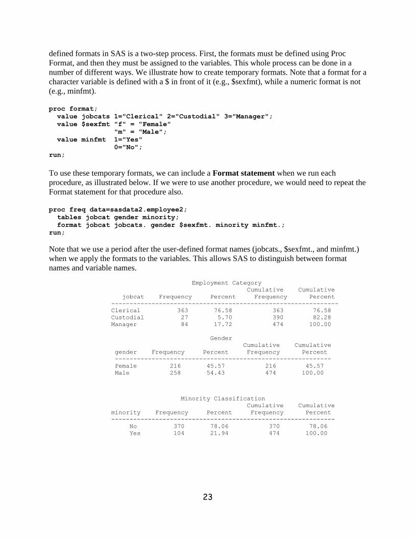
defined formats in SAS is a two-step process. First, the formats must be defined using Proc

Format, and then they must be assigned to the variables. This whole process can be done in a

number of different ways. We illustrate how to create temporary formats. Note that a format for a

character variable is defined with a $ in front of it (e.g., $sexfmt), while a numeric format is not

(e.g., minfmt).

proc format;

value jobcats 1="Clerical" 2="Custodial" 3="Manager";

value $sexfmt "f" = "Female"

"m" = "Male";

value minfmt 1="Yes"

0="No";

run;

To use these temporary formats, we can include a Format statement when we run each

procedure, as illustrated below. If we were to use another procedure, we would need to repeat the

Format statement for that procedure also.

proc freq data=sasdata2.employee2;

tables jobcat gender minority;

format jobcat jobcats. gender $sexfmt. minority minfmt.;

run;

Note that we use a period after the user-defined format names (jobcats., $sexfmt., and minfmt.)

when we apply the formats to the variables. This allows SAS to distinguish between format

names and variable names.

Employment Category

Cumulative Cumulative

jobcat Frequency Percent Frequency Percent

--------------------------------------------------------------

Clerical 363 76.58 363 76.58

Custodial 27 5.70 390 82.28

Manager 84 17.72 474 100.00

Gender


gender Frequency Percent Frequency Percent

-----------------------------------------------------------

Female 216 45.57 216 45.57

Male 258 54.43 474 100.00

Minority Classification


minority Frequency Percent Frequency Percent

-------------------------------------------------------------

No 370 78.06 370 78.06

Yes 104 21.94 474 100.00

24

Permanent Formats

Another way to assign formats so that they will apply to the variables any time they are used is to

use a format statement in a data step. This method will assign the formats to the variables at any

time they are used in the future for any procedure.

proc format lib=sasdata2;

value jobcats 1="Clerical" 2="Custodial" 3="Manager";

value $sexfmt "f" = "Female"

"m" = "Male";

value minfmt 1="Yes"

0="No";

run;

proc datasets lib=sasdata2;

modify employee2;

format jobcat jobcats. gender $sexfmt. minority minfmt.;

run;

This produces output in the SAS log that shows how the employee dataset in the sasdata2 library

has been modified.

104 proc datasets lib=sasdata2;

Directory

Libref SASDATA2

Engine V9

Physical Name C:\Users\kwelch\Desktop\sasdata2

Filename C:\Users\kwelch\Desktop\sasdata2

Member File

# Name Type Size Last Modified

1 AFIFI DATA 50176 08Dec10:11:10:13

2 AUTISM_DEMOG DATA 25600 03Mar08:10:42:22

3 AUTISM_SOCIALIZATION DATA 41984 24Jul09:06:40:00

4 BANK DATA 46080 13Jan08:19:17:04

5 BASEBALL DATA 82944 20Jun02:06:12:32

6 BUSINESS DATA 17408 20Aug06:03:05:04

7 BUSINESS2 DATA 17408 24Sep10:05:20:10

8 CARS DATA 33792 22Aug06:00:03:42

9 EMPLOYEE DATA 41984 10Jan11:13:58:24

10 EMPLOYEE2 DATA 13312 10Jan11:14:10:12

11 FITNESS DATA 9216 06Mar06:09:04:44

12 FORMATS CATALOG 17408 10Jan11:14:11:31

13 IRIS DATA 13312 20Jun02:06:12:32

14 TECUMSEH DATA 1147904 01Jun05:23:00:04

15 WAVE1 DATA 578560 20Jun07:11:11:00

16 WAVE2 DATA 492544 20Jun07:11:11:00

17 WAVE3 DATA 455680 20Jun07:11:11:00

105 modify employee2;

106 format jobcat jobcats. gender $sexfmt. minority minfmt.;

107 run;

NOTE: MODIFY was successful for SASDATA2.EMPLOYEE2.DATA.

108 quit;

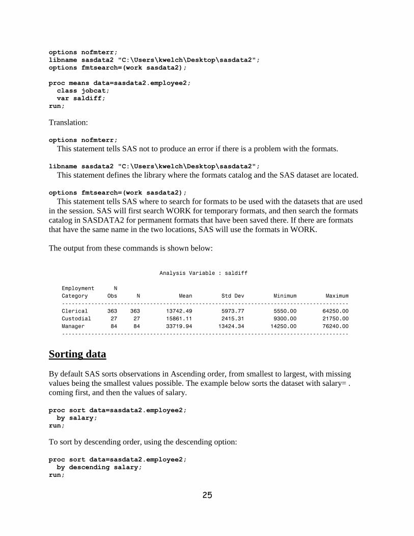
To use this dataset with the formats later, you need to use some rather arcane SAS code, shown

below:

25

options nofmterr;


options fmtsearch=(work sasdata2);

proc means data=sasdata2.employee2;

class jobcat;

var saldiff;

run;

Translation:

options nofmterr;

This statement tells SAS not to produce an error if there is a problem with the formats.


This statement defines the library where the formats catalog and the SAS dataset are located.

options fmtsearch=(work sasdata2);

This statement tells SAS where to search for formats to be used with the datasets that are used

in the session. SAS will first search WORK for temporary formats, and then search the formats

catalog in SASDATA2 for permanent formats that have been saved there. If there are formats

that have the same name in the two locations, SAS will use the formats in WORK.

The output from these commands is shown below:

Analysis Variable : saldiff

Employment N

Category Obs N Mean Std Dev Minimum Maximum

----------------------------------------------------------------------------------------

Clerical 363 363 13742.49 5973.77 5550.00 64250.00

Custodial 27 27 15861.11 2415.31 9300.00 21750.00

Manager 84 84 33719.94 13424.34 14250.00 76240.00

----------------------------------------------------------------------------------------

Sorting data

By default SAS sorts observations in Ascending order, from smallest to largest, with missing

values being the smallest values possible. The example below sorts the dataset with salary= .

coming first, and then the values of salary.

proc sort data=sasdata2.employee2;

by salary;

run;

To sort by descending order, using the descending option:


by descending salary;

run;

26

Sort by more than one variable

When sorting by more than one variable, SAS sorts based on values of the first variable, and then

it sorts based on the second variable, and so on. By default, SAS will use Ascending order for

each variable, unless otherwise specified. In the example below, the data set is first sorted in

ascending order of gender, and then within each level of gender, in descending order of salary.


by gender descending salary;

run;

Descriptive Statistics Using SAS

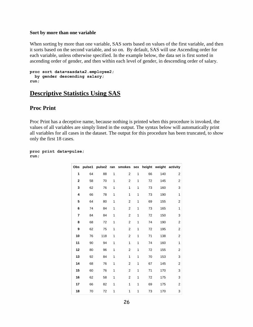
Proc Print

Proc Print has a deceptive name, because nothing is printed when this procedure is invoked, the

values of all variables are simply listed in the output. The syntax below will automatically print

all variables for all cases in the dataset. The output for this procedure has been truncated, to show

only the first 18 cases.

proc print data=pulse;

run;

Obs pulse1 pulse2 ran smokes sex height weight activity

1 64 88 1 2 1 66 140 2

2 58 70 1 2 1 72 145 2

3 62 76 1 1 1 73 160 3

4 66 78 1 1 1 73 190 1

5 64 80 1 2 1 69 155 2

6 74 84 1 2 1 73 165 1

7 84 84 1 2 1 72 150 3

8 68 72 1 2 1 74 190 2

9 62 75 1 2 1 72 195 2

10 76 118 1 2 1 71 138 2

11 90 94 1 1 1 74 160 1

12 80 96 1 2 1 72 155 2

13 92 84 1 1 1 70 153 3

14 68 76 1 2 1 67 145 2

15 60 76 1 2 1 71 170 3

16 62 58 1 2 1 72 175 3

17 66 82 1 1 1 69 175 2

18 70 72 1 1 1 73 170 3

27

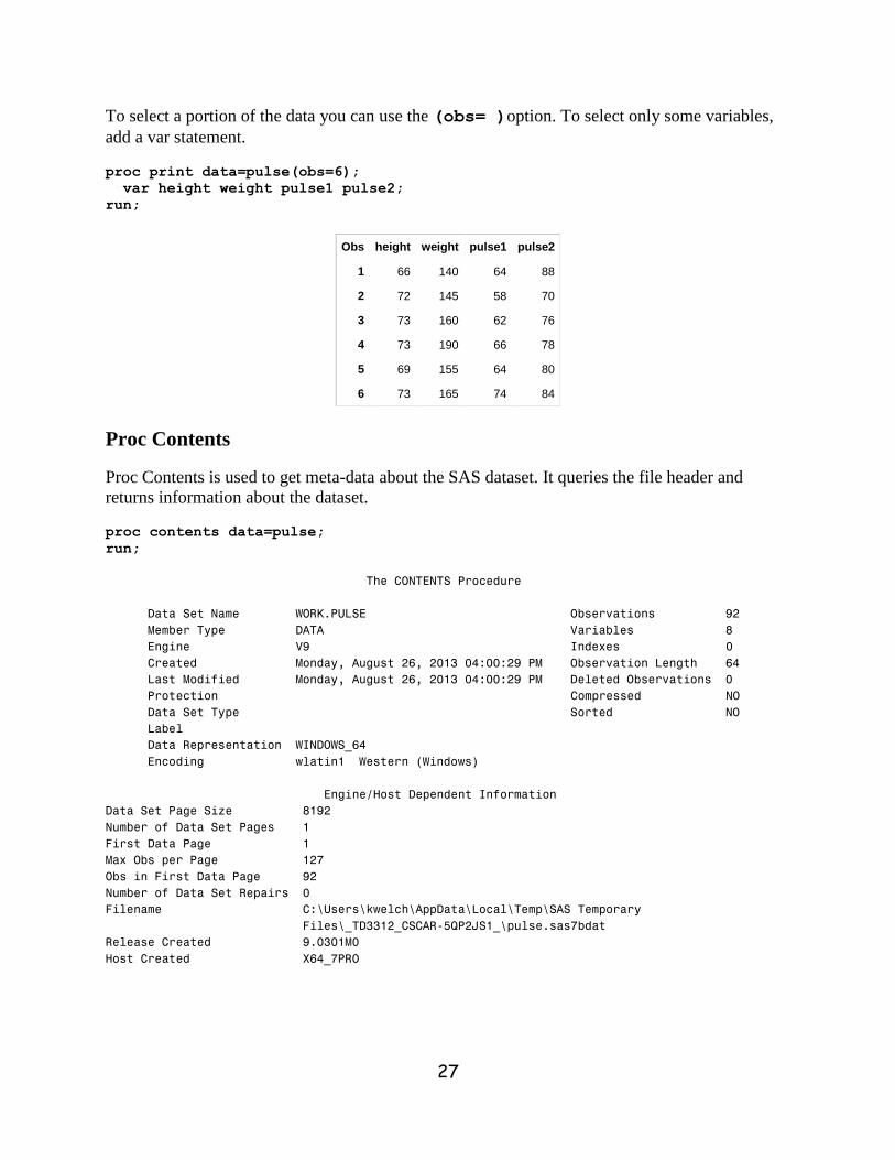
To select a portion of the data you can use the (obs= )option. To select only some variables,

add a var statement.

proc print data=pulse(obs=6);

var height weight pulse1 pulse2;

run;

Obs height weight pulse1 pulse2

1 66 140 64 88

2 72 145 58 70

3 73 160 62 76

4 73 190 66 78

5 69 155 64 80

6 73 165 74 84

Proc Contents

Proc Contents is used to get meta-data about the SAS dataset. It queries the file header and

returns information about the dataset.

proc contents data=pulse;

run;

The CONTENTS Procedure

Data Set Name WORK.PULSE Observations 92

Member Type DATA Variables 8

Engine V9 Indexes 0

Created Monday, August 26, 2013 04:00:29 PM Observation Length 64

Last Modified Monday, August 26, 2013 04:00:29 PM Deleted Observations 0

Protection Compressed NO

Data Set Type Sorted NO

Label

Data Representation WINDOWS_64

Encoding wlatin1 Western (Windows)

Engine/Host Dependent Information

Data Set Page Size 8192

Number of Data Set Pages 1

First Data Page 1

Max Obs per Page 127

Obs in First Data Page 92

Number of Data Set Repairs 0

Filename C:\Users\kwelch\AppData\Local\Temp\SAS Temporary

Files\_TD3312_CSCAR-5QP2JS1_\pulse.sas7bdat

Release Created 9.0301M0

Host Created X64_7PRO

28

Alphabetic List of Variables and Attributes

# Variable Type Len Format Label

8 activity Num 8 BEST12. activity

6 height Num 8 BEST12. height

1 pulse1 Num 8 BEST12. pulse1


3 ran Num 8 BEST12. ran

5 sex Num 8 BEST12. sex

4 smokes Num 8 BEST12. smokes

7 weight Num 8 BEST12. weight

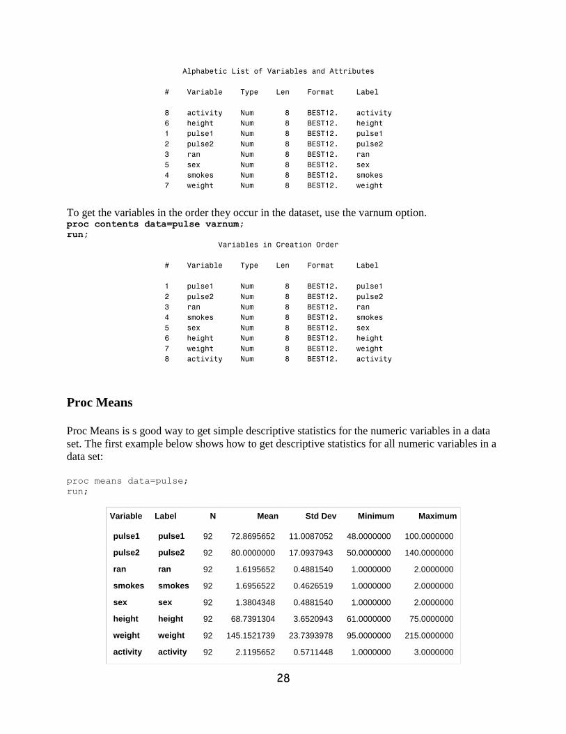
To get the variables in the order they occur in the dataset, use the varnum option. proc contents data=pulse varnum;

run;

Variables in Creation Order

# Variable Type Len Format Label



3 ran Num 8 BEST12. ran

4 smokes Num 8 BEST12. smokes

5 sex Num 8 BEST12. sex

6 height Num 8 BEST12. height

7 weight Num 8 BEST12. weight

8 activity Num 8 BEST12. activity

Proc Means

Proc Means is s good way to get simple descriptive statistics for the numeric variables in a data

set. The first example below shows how to get descriptive statistics for all numeric variables in a

data set:

proc means data=pulse;

run;

Variable Label N Mean Std Dev Minimum Maximum

pulse1

pulse2

ran

smokes

sex

height

weight

activity

pulse1

pulse2

ran

smokes

sex

height

weight

activity

92

92

92

92

92

92

92

92

72.8695652

80.0000000

1.6195652

1.6956522

1.3804348

68.7391304

145.1521739

2.1195652

11.0087052

17.0937943

0.4881540

0.4626519

0.4881540

3.6520943

23.7393978

0.5711448

48.0000000

50.0000000

1.0000000

1.0000000

1.0000000

61.0000000

95.0000000

1.0000000

100.0000000

140.0000000

2.0000000

2.0000000

2.0000000

75.0000000

215.0000000

3.0000000

29

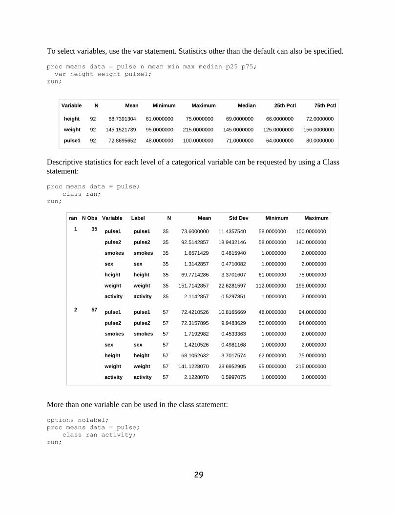
To select variables, use the var statement. Statistics other than the default can also be specified.

proc means data = pulse n mean min max median p25 p75;

var height weight pulse1;

run;

Variable N Mean Minimum Maximum Median 25th Pctl 75th Pctl

height

weight

pulse1

92

92

92

68.7391304

145.1521739

72.8695652

61.0000000

95.0000000

48.0000000

75.0000000

215.0000000

100.0000000

69.0000000

145.0000000

71.0000000

66.0000000

125.0000000

64.0000000

72.0000000

156.0000000

80.0000000

Descriptive statistics for each level of a categorical variable can be requested by using a Class

statement:

proc means data = pulse;

class ran;

run;

ran N Obs Variable Label N Mean Std Dev Minimum Maximum

1 35 pulse1

pulse2

smokes

sex

height

weight

activity

pulse1

pulse2

smokes

sex

height

weight

activity

35

35

35

35

35

35

35

73.6000000

92.5142857

1.6571429

1.3142857

69.7714286

151.7142857

2.1142857

11.4357540

18.9432146

0.4815940

0.4710082

3.3701607

22.6281597

0.5297851

58.0000000

58.0000000

1.0000000

1.0000000

61.0000000

112.0000000

1.0000000

100.0000000

140.0000000

2.0000000

2.0000000

75.0000000

195.0000000

3.0000000

2 57 pulse1

pulse2

smokes

sex

height

weight

activity

pulse1

pulse2

smokes

sex

height

weight

activity

57

57

57

57

57

57

57

72.4210526

72.3157895

1.7192982

1.4210526

68.1052632

141.1228070

2.1228070

10.8165669

9.9483629

0.4533363

0.4981168

3.7017574

23.6952905

0.5997075

48.0000000

50.0000000

1.0000000

1.0000000

62.0000000

95.0000000

1.0000000

94.0000000

94.0000000

2.0000000

2.0000000

75.0000000

215.0000000

3.0000000

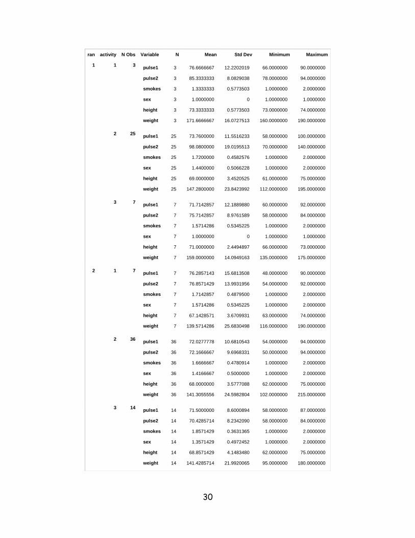
More than one variable can be used in the class statement:

options nolabel;

proc means data = pulse;

class ran activity;

run;

30

ran activity N Obs Variable N Mean Std Dev Minimum Maximum

1 1 3 pulse1

pulse2

smokes

sex

height

weight

3

3

3

3

3

3

76.6666667

85.3333333

1.3333333

1.0000000

73.3333333

171.6666667

12.2202019

8.0829038

0.5773503

0

0.5773503

16.0727513

66.0000000

78.0000000

1.0000000

1.0000000

73.0000000

160.0000000

90.0000000

94.0000000

2.0000000

1.0000000

74.0000000

190.0000000

2 25 pulse1

pulse2

smokes

sex

height

weight

25

25

25

25

25

25

73.7600000

98.0800000

1.7200000

1.4400000

69.0000000

147.2800000

11.5516233

19.0195513

0.4582576

0.5066228

3.4520525

23.8423992

58.0000000

70.0000000

1.0000000

1.0000000

61.0000000

112.0000000

100.0000000

140.0000000

2.0000000

2.0000000

75.0000000

195.0000000

3 7 pulse1

pulse2

smokes

sex

height

weight

7

7

7

7

7

7

71.7142857

75.7142857

1.5714286

1.0000000

71.0000000

159.0000000

12.1889880

8.9761589

0.5345225

0

2.4494897

14.0949163

60.0000000

58.0000000

1.0000000

1.0000000

66.0000000

135.0000000

92.0000000

84.0000000

2.0000000

1.0000000

73.0000000

175.0000000

2 1 7 pulse1

pulse2

smokes

sex

height

weight

7

7

7

7

7

7

76.2857143

76.8571429

1.7142857

1.5714286

67.1428571

139.5714286

15.6813508

13.9931956

0.4879500

0.5345225

3.6709931

25.6830498

48.0000000

54.0000000

1.0000000

1.0000000

63.0000000

116.0000000

90.0000000

92.0000000

2.0000000

2.0000000

74.0000000

190.0000000

2 36 pulse1

pulse2

smokes

sex

height

weight

36

36

36

36

36

36

72.0277778

72.1666667

1.6666667

1.4166667

68.0000000

141.3055556

10.6810543

9.6968331

0.4780914

0.5000000

3.5777088

24.5982804

54.0000000

50.0000000

1.0000000

1.0000000

62.0000000

102.0000000

94.0000000

94.0000000

2.0000000

2.0000000

75.0000000

215.0000000

3 14 pulse1

pulse2

smokes

sex

height

weight

14

14

14

14

14

14

71.5000000

70.4285714

1.8571429

1.3571429

68.8571429

141.4285714

8.6000894

8.2342090

0.3631365

0.4972452

4.1483480

21.9920065

58.0000000

58.0000000

1.0000000

1.0000000

62.0000000

95.0000000

87.0000000

84.0000000

2.0000000

2.0000000

75.0000000

180.0000000

31

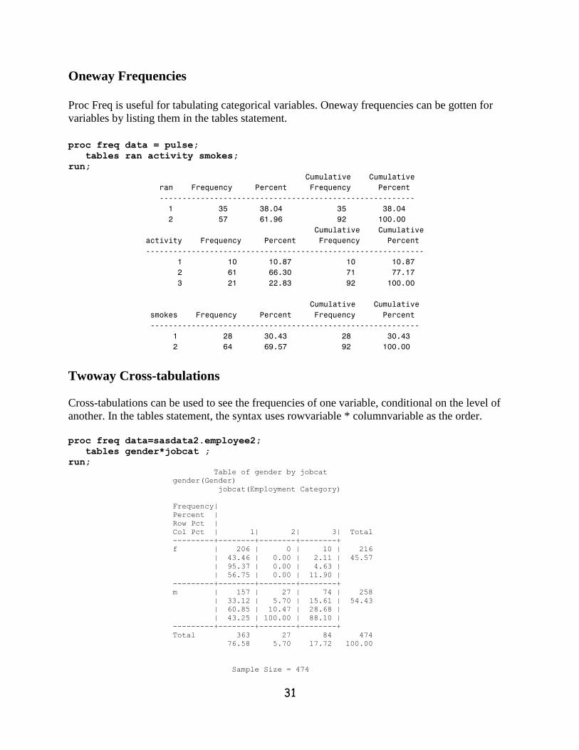
Oneway Frequencies

Proc Freq is useful for tabulating categorical variables. Oneway frequencies can be gotten for

variables by listing them in the tables statement.

proc freq data = pulse;

tables ran activity smokes;

run;


ran Frequency Percent Frequency Percent

--------------------------------------------------------

1 35 38.04 35 38.04

2 57 61.96 92 100.00


activity Frequency Percent Frequency Percent

-------------------------------------------------------------

1 10 10.87 10 10.87

2 61 66.30 71 77.17

3 21 22.83 92 100.00


smokes Frequency Percent Frequency Percent

-----------------------------------------------------------

1 28 30.43 28 30.43

2 64 69.57 92 100.00

Twoway Cross-tabulations

Cross-tabulations can be used to see the frequencies of one variable, conditional on the level of

another. In the tables statement, the syntax uses rowvariable * columnvariable as the order.

proc freq data=sasdata2.employee2;

tables gender*jobcat ;

run; Table of gender by jobcat

gender(Gender)

jobcat(Employment Category)

Frequency|

Percent |

Row Pct |

Col Pct | 1| 2| 3| Total

---------+--------+--------+--------+

f | 206 | 0 | 10 | 216

| 43.46 | 0.00 | 2.11 | 45.57

| 95.37 | 0.00 | 4.63 |

| 56.75 | 0.00 | 11.90 |

---------+--------+--------+--------+

m | 157 | 27 | 74 | 258

| 33.12 | 5.70 | 15.61 | 54.43

| 60.85 | 10.47 | 28.68 |

| 43.25 | 100.00 | 88.10 |

---------+--------+--------+--------+

Total 363 27 84 474

76.58 5.70 17.72 100.00

Sample Size = 474

32

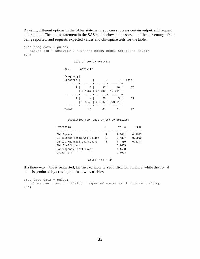
By using different options in the tables statement, you can suppress certain output, and request

other output. The tables statement in the SAS code below suppresses all of the percentages from

being reported, and requests expected values and chi-square tests for the table.


tables sex * activity / expected norow nocol nopercent chisq;

run;

Table of sex by activity

sex activity

Frequency|

Expected | 1| 2| 3| Total

---------+--------+--------+--------+

1 | 6 | 35 | 16 | 57

| 6.1957 | 37.793 | 13.011 |

---------+--------+--------+--------+

2 | 4 | 26 | 5 | 35

| 3.8043 | 23.207 | 7.9891 |

---------+--------+--------+--------+

Total 10 61 21 92

Statistics for Table of sex by activity

Statistic DF Value Prob

------------------------------------------------------

Chi-Square 2 2.3641 0.3067

Likelihood Ratio Chi-Square 2 2.4827 0.2890

Mantel-Haenszel Chi-Square 1 1.4339 0.2311

Phi Coefficient 0.1603

Contingency Coefficient 0.1583

Cramer's V 0.1603

Sample Size = 92

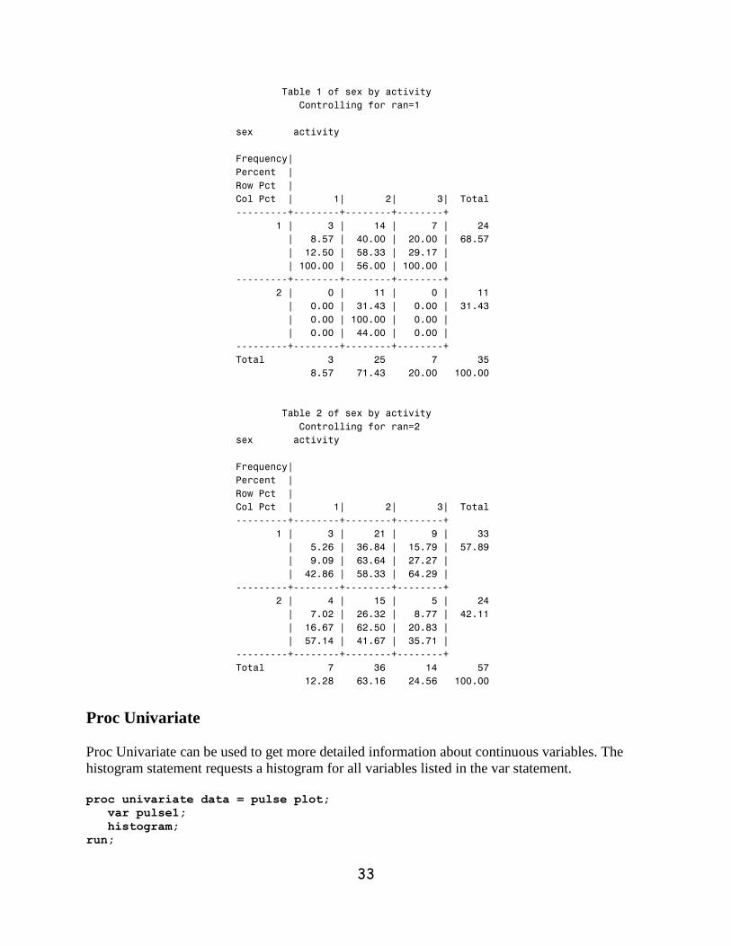
If a three-way table is requested, the first variable is a stratification variable, while the actual

table is produced by crossing the last two variables.


tables ran * sex * activity / expected norow nocol nopercent chisq;

run;

33

Table 1 of sex by activity

Controlling for ran=1

sex activity

Frequency|

Percent |

Row Pct |


---------+--------+--------+--------+

1 | 3 | 14 | 7 | 24

| 8.57 | 40.00 | 20.00 | 68.57

| 12.50 | 58.33 | 29.17 |

| 100.00 | 56.00 | 100.00 |

---------+--------+--------+--------+

2 | 0 | 11 | 0 | 11

| 0.00 | 31.43 | 0.00 | 31.43

| 0.00 | 100.00 | 0.00 |

| 0.00 | 44.00 | 0.00 |

---------+--------+--------+--------+

Total 3 25 7 35

8.57 71.43 20.00 100.00

Table 2 of sex by activity

Controlling for ran=2

sex activity

Frequency|

Percent |

Row Pct |


---------+--------+--------+--------+

1 | 3 | 21 | 9 | 33

| 5.26 | 36.84 | 15.79 | 57.89

| 9.09 | 63.64 | 27.27 |

| 42.86 | 58.33 | 64.29 |

---------+--------+--------+--------+

2 | 4 | 15 | 5 | 24

| 7.02 | 26.32 | 8.77 | 42.11

| 16.67 | 62.50 | 20.83 |

| 57.14 | 41.67 | 35.71 |

---------+--------+--------+--------+

Total 7 36 14 57

12.28 63.16 24.56 100.00

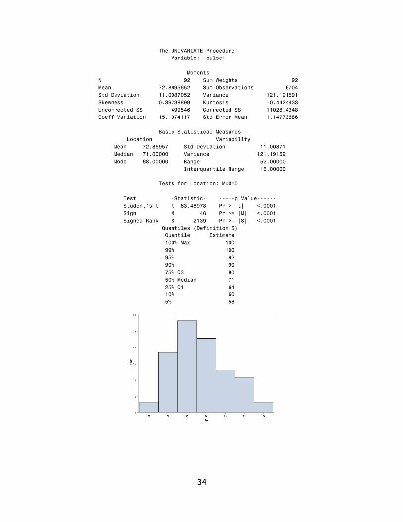
Proc Univariate

Proc Univariate can be used to get more detailed information about continuous variables. The

histogram statement requests a histogram for all variables listed in the var statement.

proc univariate data = pulse plot;

var pulse1;

histogram;

run;

34

The UNIVARIATE Procedure

Variable: pulse1

Moments

N 92 Sum Weights 92

Mean 72.8695652 Sum Observations 6704

Std Deviation 11.0087052 Variance 121.191591

Skewness 0.39738899 Kurtosis -0.4424433

Uncorrected SS 499546 Corrected SS 11028.4348

Coeff Variation 15.1074117 Std Error Mean 1.14773686

Basic Statistical Measures

Location Variability

Mean 72.86957 Std Deviation 11.00871

Median 71.00000 Variance 121.19159

Mode 68.00000 Range 52.00000

Interquartile Range 16.00000

Tests for Location: Mu0=0

Test -Statistic- -----p Value------

Student's t t 63.48978 Pr > |t| <.0001

Sign M 46 Pr >= |M| <.0001

Signed Rank S 2139 Pr >= |S| <.0001

Quantiles (Definition 5)

Quantile Estimate

100% Max 100

99% 100

95% 92

90% 90

75% Q3 80

50% Median 71

25% Q1 64

10% 60

5% 58

35

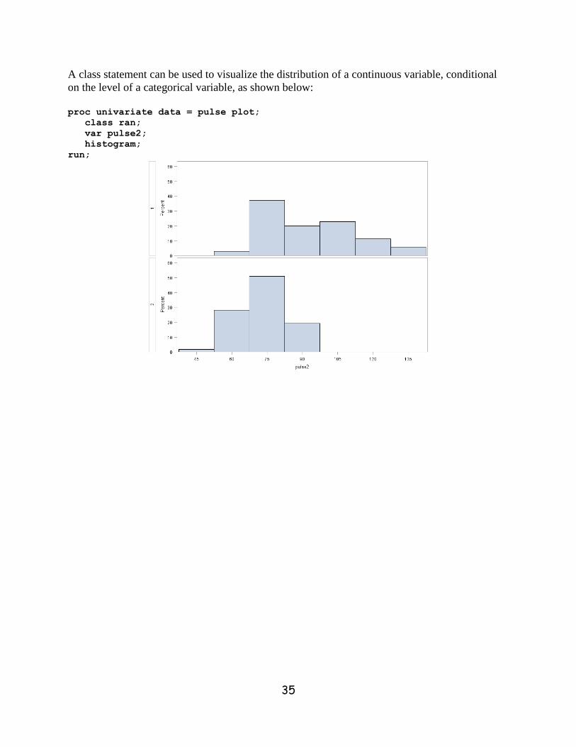
A class statement can be used to visualize the distribution of a continuous variable, conditional

on the level of a categorical variable, as shown below:

proc univariate data = pulse plot;

class ran;

var pulse2;

histogram;

run;

Documents

A Brief Tour of SAS - Personal Web Server