Embed Size (px)
Citation preview
A burn-through model for textile membranes in buildings as a tool in performance based fire
safety engineering
Petra Andersson, Joel Andersson, Andreas Lennqvist, Heimo Tuovinen and Per Blomqvist
Fire Technology
SP Report 2010:54
SP
Tec
hnic
al R
esea
rch
Inst
itute
of S
wed
en
A burn-through model for textile membranes in buildings as a tool in performance based fire safety engineering Petra Andersson, Joel Andersson, Andreas Lennqvist, Heimo Tuovinen and Per Blomqvist
3
Abstract This work has been conducted within the European project contex-T, “Textile Architecture – Textile Structures and Buildings of the Future”. Contex-T is an Integrated Project dedicated to SMEs within the 6th Framework Programme and brings together a consortium of over 30 partners from 10 countries. Among the main objectives of the project is the development of new lightweight buildings using textile structures and the development of safe, healthy and economic buildings. Advantages of textile materials in buildings includes their low weight, and in the case of textile membranes, their translucency and architectural possibilities. A common disadvantage, however, is the fire properties of textile materials which highlights the importance of fire safety assessments for building application of such materials. This report describes the work conducted to model the opening up of a hole in a textile membrane due to fire. The work has been conducted using the CFD code FDS utilising the burn away option. Two different PVC-PES membranes were used. Input data were determined from Cone Calorimeter, TGA and TPS measurements. The simulations were validated against full scale experiments. In addition, the use of the model was demonstrated on two of the contex-T demonstrators, i.e. the VUB and Wagner building. The study showed that it is possible to use the burn away option to open up a hole in the membrane due to fire, but the simulations contain large uncertainties as it is difficult to determine the input parameters due to experimental uncertainties and the fact that hole opening is a complex phenomenon including processes such as cracks due to weakening of the material by heat, etc. Key words: contex-T, textile membranes, fire, CFD modelling, burn-through, FDS SP Sveriges Tekniska Forskningsinstitut SP Technical Research Institute of Sweden SP Report 2010:54 ISBN 978-91-86319-94-6 ISSN 0284-5172 Borås 2010
4
Contents
Abstract 3
Contents 4
Preface 5
Sammanfattning 6
1 Introduction 7
2 Method 8
3 The simulation tool and its utility programs 9
4 FDS 10 4.1 The BURN_AWAY option 10 4.2 Pyrolysis models 10 4.2.1 Model I: Solid Fuels that Burn at a Specified Rate 10 4.2.2 Model II: Solid Fuels that do NOT Burn at a Specified Rate 11
5 Validation experiments 12
6 Input in FDS – Material parameters 14
7 Simulations of validation experiment 17 7.1 Pyrolysis model I – Prescribed burning rate 18 7.1.1 Grid independency 28 7.1.2 Differences between computers 29 7.2 Pyrolysis model II 30 7.3 Comparison discussion 36
8 Application – Demonstration buildings 39 8.1 The VUB-building 39 8.2 The Wagner building 41 8.3 Discussion 43
9 Simulation of double membrane 44
10 Discussion 46 10.1 Further studies 47
11 Conclusions 48
References 49
Appendix A - Fire Safety Engineering in contex-T 50

5
Preface This work is part of the contex-T project, a EU sponsored project within the 6th Framework Programme with contract no 26574. We are grateful to the contex-T consortium for allowing the publication of this contex-T report in the form of a SP Report. Part of the funding was obtained from BRANDFORSK project nr 307-071.
6
Summary This report describes the work conducted to model the opening up of a hole in a textile membrane due to fire. The work has been conducted using the CFD code FDS utilising the burn away option. Two different PVC-PES membranes were used. Input data were determined from Cone Calorimeter, TGA and TPS measurements. The simulations were validated against full scale experiments. In addition, the use of the model was demonstrated on two of the contex-T demonstrators, i.e. the VUB and Wagner building. The study showed that it is possible to use the burn away option to open up a hole in the membrane due to fire, but the simulations contain large uncertainties as it is difficult to determine the input parameters due to experimental uncertainties and the fact that hole opening is a complex phenomenon including processes such as cracks due to weakening of the material by heat, etc.
7
1 Introduction The main objective of the contex-T project is the development of new lightweight buildings using textile structures and the development of safe, healthy and economic buildings. Advantages of textile materials in buildings include their low weight, and in the case of textile membranes, their translucency and architectural potential. A common disadvantage, however, is the fire performance of the textile materials which highlights the importance of fire safety assessments for building applications of such materials. Textile membranes are today used in different types of building applications. There are examples of applications for sport arenas, such as the Commertzbank Arena in Frankfurt where textile membranes are used as roofing material and the Allianz Arena in Munich where textile membranes are used both as roofing and wall materials. The new International Airport in Bangkok is another example of an advanced application of textile membranes as building material for a permanent building. Other possible applications include exhibition halls, hangars and functional/decorative building components such as room dividers and detached ceilings in atriums. Advantages of textile materials in buildings includes the low weight, and in the case of textile membranes, their translucency and architectural possibilities. A common disadvantage, however, are the fire properties of textile materials which highlights the importance of fire safety design for building application of such materials. Prescriptive fire safety regulations, which in detail describe the design and classification of building components, will exclude the use of textile materials for applications where the materials will not conform to the required fire rating. A performance based approach to comply with the overall fire safety level of the building can be a valid alternative for certain applications. Fire safety engineering and the work conducted within contex-T is described in Appendix A. Computational Fluid Dynamics (CFD) simulations are an important tool for justifying performance based design solutions. One important aspect when it comes to buildings constructed using textile membranes is that such buildings can obtain natural smoke ventilation if a hole opens up in the membrane during a fire. This feature must therefore be included in CFD-models when used for simulations of textile membranes in fires. This report presents a method in which the burn away option in Fire Dynamics Simulator (FDS), a Large Eddy CFD code developed by NIST, is used to mimic this feature.
8
2 Method Smoke venting is one important fire safety measure in order to provide safe evacuation of a building in case of a fire as the smoke venting gives the occupants a longer time to evacuate. Smoke venting is in many cases accomplished by special smoke vents that open when the temperature of a trigger device reaches a certain temperature (often about 70°C) for industrial applications or when a smoke detector activates in buildings were many people are present. When the smoke vent is opened then normally also a door or something else is opened to supply air in order to get the smoke flowing out of the building. There are several CFD codes available on the market. Lately, one code has become dominant in Fire Safety Engineering applications as it is a shareware, i.e. the Fire Dynamics Simulator (FDS) code developed by NIST 1. This was the main reason for choosing it for this study. The feature of opening a smoke vent with a trigger device is included in FDS. Using this feature was, however, not considered as a viable option as this would require specification of a trigger device for each cell if one would like to simulate both time to hole opening and the size of the hole as it grows during the fire. Therefore it was decided to use an option in FDS that is called the burn away option to try to mimic the opening up a hole in the membrane. The study was conducted on two different PVC-PESi membranes, one thin, about 0.5 mm thick, and one thicker, about 1 mm thick. The work started using a simple pyrolysis model that requires an ignition temperature and a user prescribed burning rate as it was deemed that this model would be easier to use for a typical user. Input parameters were determined from Cone Calorimeter experiments and initial simulations of the Cone Calorimeter tests were conducted. A set of full scale validation tests were conducted and the model was validated against these and a parametric study was conducted. Based on this validation it was decided to test the more complex pyrolysis model also. Input parameters for this were obtained from TGA measurements. The possibility to use the model on realistic buildings was demonstrated by using the model on two of the projects demonstrator buildings, i.e. the VUB building and the Wagner building. In addition, the possibility of applying the model to a double membrane building was investigated. For these latter cases there are, however, no validation experiments to compare with the results of the simulations.
i PVC-PES = Textile membrane with polivinyl chloride (PVC) coating on a polyester (PES) backing.
9
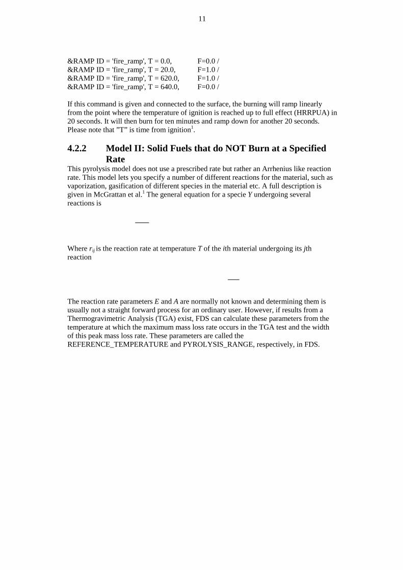
3 The simulation tool and its utility programs The FDS package comprises of FDS itself and Smokeview that is used to display output data. FDS itself does not have a user interface, all input data needs to be specified in a text file written according to a required format. There are, however, a number of third party programs available to help the user to construct input files and evaluate e.g. smoke detectors. One example is Pyrosim that can be used to e.g. construct the mesh for more complex geometries. Pyrosim helps the user create the FDS input via a graphical interface. Some of the features of Pyrosim include a number of drawing tools, the constant view of the geometry and the possibility to import 2D and 3D AutoCAD DXF files or existing FDS files 2. The importing feature is especially usable when dealing with complex geometries which would be both time consuming and difficult to write manually in a text file. Smokeview 3 is used to visualize the results. Smokeview reads the FDS output data and produces pictures based on this information. An example is presented in Figure1 where one can see the simulation domain without a fire. The domain consists of a room with a door opening. The fire starts in the middle of the room, about one meter above the floor. The green dots show where the user has specified measurement devices, which are useful in evaluating (or validating) the simulation results.
Figure 1 Smokeview picture of the geometry in FDS.
10
4 FDS Fire Dynamics Simulator (FDS) solves Navier-Stokes equations and is well suited for simulating low speed thermally-driven flows such as those produced by a fire and smoke. The turbulence is calculated using the Smagorinsky form of Large Eddy Simulation (LES). FDS is widely used for performance based fire safety design. It reads input parameters from a text file, computes according to the governing equations and writes the sought data to files. The program includes several sub-models for modeling combustion, radiation, water droplet trajectories, heat transfer, pyrolysis, etc1. FDS is under constant development and the currently latest version, version 5.5.0 was released in April 2010. FDS can only handle one gaseous fuel. The default fuel is propane if no other fuel is specified. A FDS simulation can, however, include several different solid and liquid phase fuels, but these needs to be translated into a single gaseous fuel once they have gasified and begun to burn. 4.1 The BURN_AWAY option The BURN_AWAY option in FDS removes a cell of a burning object from the calculation once it is consumed. It can be used with either of the two pyrolysis models, i.e., the simple one where the Heat Release Rate is prescribed by the user, or the more advanced using an Arrhenius expression for the reaction rate. One important correction factor when using the burn away option on a membrane that is thinner than the grid size is the BULK_DENSITY, which determines how much of the material that disappears. The BULK_DENSITY is the material density scaled by the ratio between the grid size and the membrane thickness and the ratio between the Heat of Combustion (HC) of the fuel and the effective Heat of combustion of the membrane, i.e.:
4.2 Pyrolysis models FDS contains two different pyrolysis models for solid fuels, one where the fuel is consumed at a user specified rate and one where the fuel is consumed according to a reaction rate calculated by the program. The burn away option can be used with either of the models1. 4.2.1 Model I: Solid Fuels that Burn at a Specified Rate This pyrolysis model uses a prescribed burn rate, where the material disappears with heat release per unit area (HRRPUA) when the ignition temperature is reached at the surface. When using this pyrolysis model the parameters ignition temperature (IGNITION_TEMPERATURE) and heat release rate per unit area (HRRPUA) needs to be prescribed. The membrane will neither burn nor pyrolyse before it reaches the ignition temperature. When this temperature is reached it will immediately burn off at the rate prescribed by HRRPUA. If ignition temperature is not prescribed the burn rate will immediately go to HRRPUA when the simulation starts. When specifying the HRRPUA parameter the burning rate is controlled instead of being calculated by FDS. There is a possibility to “ramp” the burning linearly by prescribing command lines similar to:
11
&RAMP ID = 'fire_ramp', T = 0.0, F=0.0 / &RAMP ID = 'fire_ramp', T = 20.0, F=1.0 / &RAMP ID = 'fire_ramp', T = 620.0, F=1.0 / &RAMP ID = 'fire_ramp', T = 640.0, F=0.0 / If this command is given and connected to the surface, the burning will ramp linearly from the point where the temperature of ignition is reached up to full effect (HRRPUA) in 20 seconds. It will then burn for ten minutes and ramp down for another 20 seconds. Please note that ”T” is time from ignition1. 4.2.2 Model II: Solid Fuels that do NOT Burn at a Specified
Rate This pyrolysis model does not use a prescribed rate but rather an Arrhenius like reaction rate. This model lets you specify a number of different reactions for the material, such as vaporization, gasification of different species in the material etc. A full description is given in McGrattan et al.1 The general equation for a specie Y undergoing several reactions is
Where rij is the reaction rate at temperature T of the ith material undergoing its jth reaction
The reaction rate parameters E and A are normally not known and determining them is usually not a straight forward process for an ordinary user. However, if results from a Thermogravimetric Analysis (TGA) exist, FDS can calculate these parameters from the temperature at which the maximum mass loss rate occurs in the TGA test and the width of this peak mass loss rate. These parameters are called the REFERENCE_TEMPERATURE and PYROLYSIS_RANGE, respectively, in FDS.
12
5 Validation experiments Four validation tests were conducted using two different membranes. The tests were conducted using a room of size 3.60 m × 2.40 m × 2.40 m, with a centrally placed door opening on the short side with an opening size of 0.8 m × 2 m. The dimensions of the test room were the same as these specified for sandwich panels in ISO 13784 4 and for surface lining materials in ISO 9705 5. A complete description of the tests is given in Andersson and Blomqvist 6. The tests conducted are summarized in Table 1. Table 1 Tests conducted.
Test number
Textile membrane
Burner location Burner stages Notes on burn-through
7 B8103/ PVC-PES / 650 g.m-2
1.0 m above floor level
95 kW – 5 min 140 kW – 5 min
Burn-through during 95 kW exposure
8 B8103/ PVC-PES / 650 g.m-2
0.45 m above floor level
95 kW – 10 min 140 kW – 10 min 300 kW – 5 min
Burn-through during 300 kW exposure
9 T3107 / PVC-PES / 1150 g.m-2
1.0 m above floor level
95 kW – 5 min 140 kW – 5 min
Burn-through during 95 kW exposure
10 T3107/ PVC-PES / 1150 g.m-2
0.45 m above floor level
95 kW – 10 min 140 kW – 10 min 300 kW – 5 min
Burn-through during 300 kW exposure
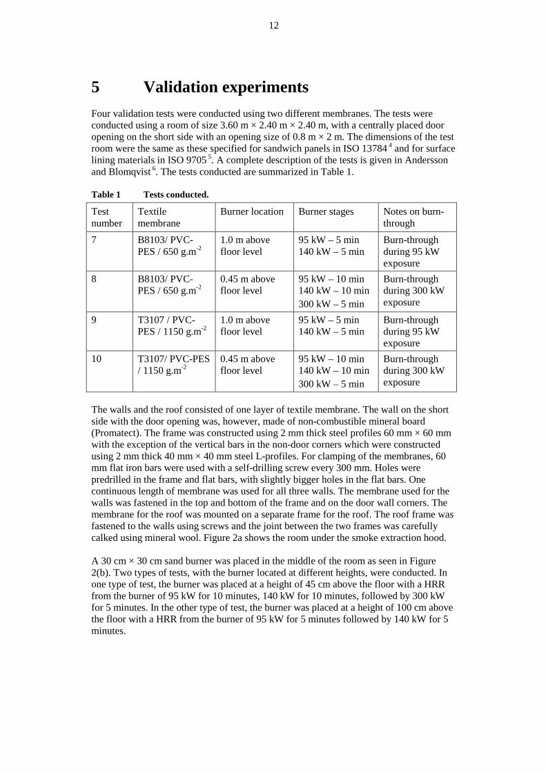
The walls and the roof consisted of one layer of textile membrane. The wall on the short side with the door opening was, however, made of non-combustible mineral board (Promatect). The frame was constructed using 2 mm thick steel profiles 60 mm × 60 mm with the exception of the vertical bars in the non-door corners which were constructed using 2 mm thick 40 mm × 40 mm steel L-profiles. For clamping of the membranes, 60 mm flat iron bars were used with a self-drilling screw every 300 mm. Holes were predrilled in the frame and flat bars, with slightly bigger holes in the flat bars. One continuous length of membrane was used for all three walls. The membrane used for the walls was fastened in the top and bottom of the frame and on the door wall corners. The membrane for the roof was mounted on a separate frame for the roof. The roof frame was fastened to the walls using screws and the joint between the two frames was carefully calked using mineral wool. Figure 2a shows the room under the smoke extraction hood. A 30 cm × 30 cm sand burner was placed in the middle of the room as seen in Figure 2(b). Two types of tests, with the burner located at different heights, were conducted. In one type of test, the burner was placed at a height of 45 cm above the floor with a HRR from the burner of 95 kW for 10 minutes, 140 kW for 10 minutes, followed by 300 kW for 5 minutes. In the other type of test, the burner was placed at a height of 100 cm above the floor with a HRR from the burner of 95 kW for 5 minutes followed by 140 kW for 5 minutes.
13
(a) (b) Figure 2 (a) The test set-up for the large-scale tests with textile membranes conforming
to the size of the ISO 9705 room, 2.4 m × 2.4 m × 3.6 m, and (b) the position of the burner in the centre of the room in one of the validation experiments.
The temperature and velocities in the door opening were measured. The temperature at 0, 10, 20, 30, 40, 50, 60, 70, 80, 90 and 100 cm below the soffit in the door opening and velocities at 10, 30 and 50 cm below the soffit, were recorded. In addition, the temperature of the membrane was measured using thermocouples (TCs) in the centre of the ceiling/roof. The TC on the membrane was mounted by the means of tape only which implies that the TC might lose contact with the membrane during the tests, especially the TC taped to the ceiling, i.e. inside the room. A thermocouple tree was located 80 cm from the rear wall, with TCs every 10 cm starting at 10 cm above the floor, up to 230 cm above floor level. In addition, one Plate Thermocouple7 was placed on the floor, 15 cm × 15 cm away from the TC tree. A simple smoke measurement, using a diode laser and a photo diode, was positioned 60 cm from the rear wall, 1.6 m above ground. Markings were made on the roof/ceiling 30 and 50 cm distance from the centre to follow the hole opening during each test. The test room was placed under a large calorimetric hood/duct system. Heat Release Rate (HRR) and smoke production were measured in the duct. Additionally, the velocities and temperature readings in the door opening were used to estimate the convective flow of heat out of the door opening. The experiments were video-recorded and photographed every 10s. The time to a hole opened up was noted and the size of the hole was measured after each experiment.
14
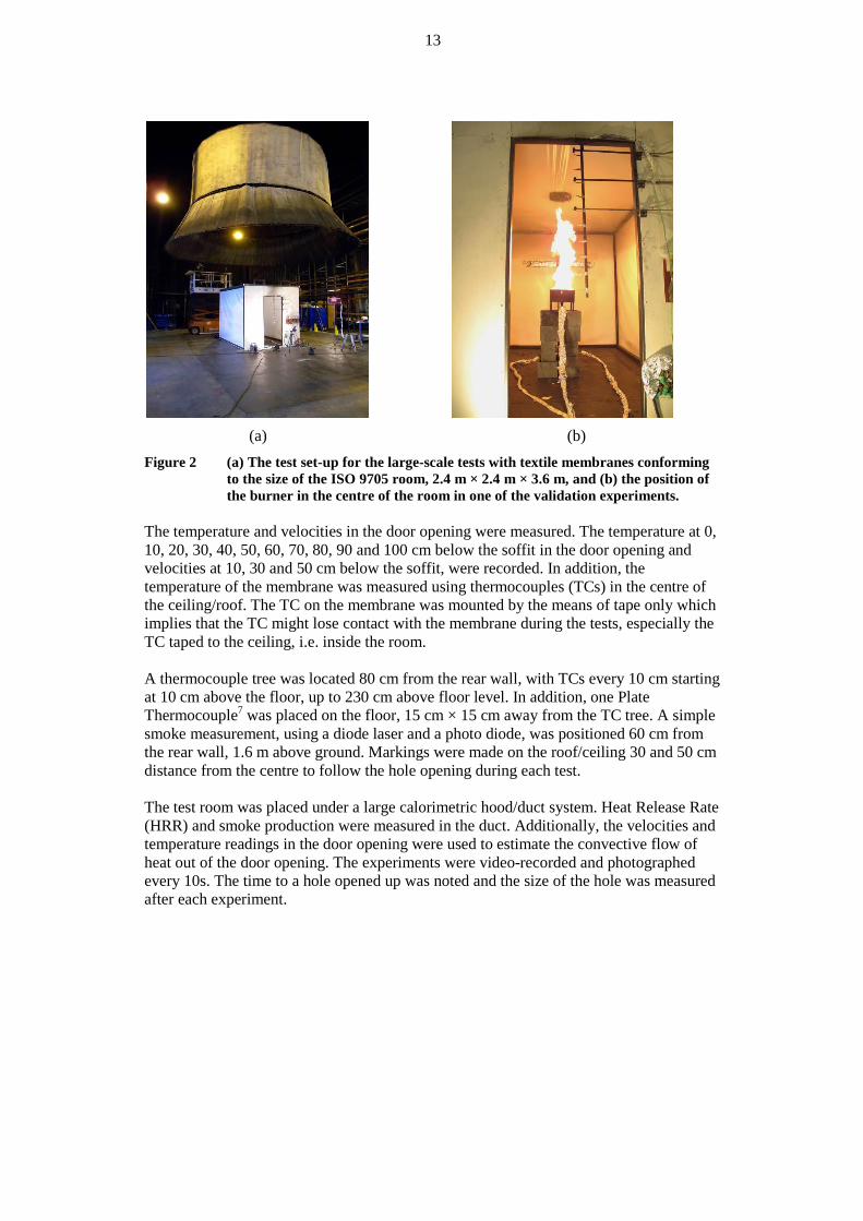
6 Input in FDS – Material parameters Two membranes were tested and simulated as listed in Table 2. Some of the material parameters used were given by the manufacturer of the membranes while some had to be determined using the Cone Calorimeter 8, Transient Plane Source (TPS) 9 and TGA. The membrane was tested in the Cone Calorimeter mounted on a non-combustible frame without any insulation on the backside. The tests were conducted without a spark-igniter and measurements were taken every second. The time to creation of a hole in the membrane was noted in all tests. In addition to the standard measurements such a mass loss and HRR, two thermocouples were mounted at the centre of the membrane, one on the exposed side and one on the backside. A photo of the mounting is shown in Figure 3. An example of temperature reading output is given in Figure 4. The tests were conducted both in the (normal) horizontal position and the vertical position. Table 2 Materials.
Material Density [kg/m3] Thickness [mm] (A) Sioen B8103/ PVC-PES 650 0.5 (D) Sioen B6656 / PVC-PES 1300 1.1 (H) Sioen T3107 / PVC-PES 1045 1.1
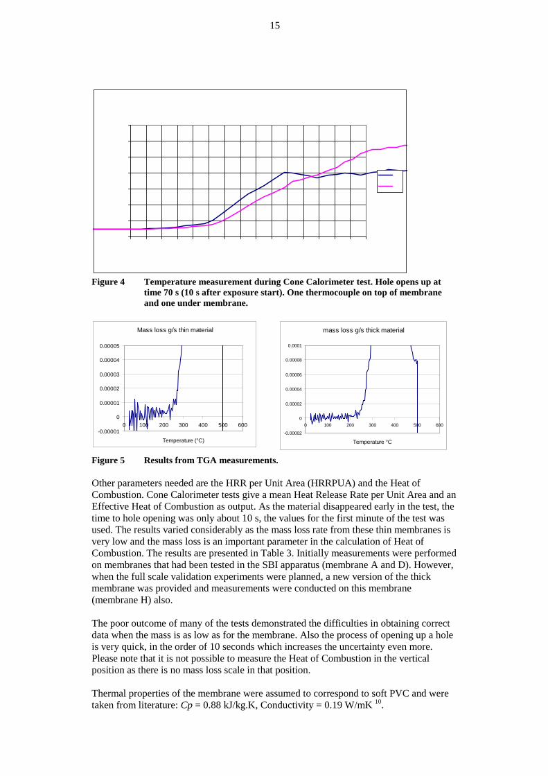
Figure 3 Mounting of membrane seen from below. The tests indicated that the membrane opened up a hole at a surface temperature of 150 – 240 °C for the thin membrane and 150 – 320 °C for the thicker membrane. However, as the burn away at a prescribed rate option in FDS needs a discrete temperature when the material starts to emit gases from the surface it was decided to run the membrane also in the TGA. The membranes were run at a temperature increase of 5 K/min in nitrogen. The measurements resulted in a pyrolysis temperature slightly above 300°C in both cases. However, as we need to know at what temperature the material starts to disappear from the surface it was decided to study when the mass loss became positive in the TGA measurements. This resulted in a temperature of 150 – 230 °C for the thin material and 200 – 230 °C for the thick material, as seen in Figure 5. This mass loss at lower temperatures, compared with the pyrolysis temperature, may partly be due to the release of plasticizers and partly due to the release of chlorine as HCl. As the temperature coincides with the temperatures achieved from the Cone Calorimeter experiments they are deemed to be relevant for this application.
15
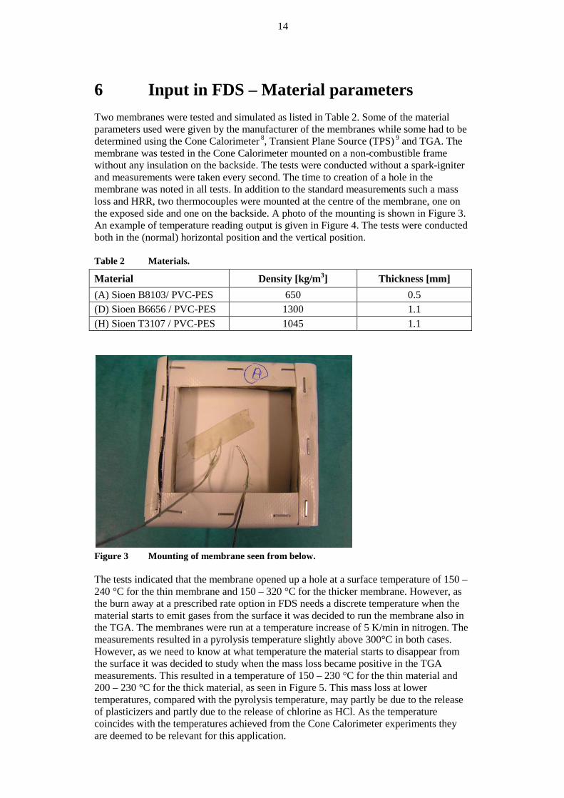
Figure 4 Temperature measurement during Cone Calorimeter test. Hole opens up at
time 70 s (10 s after exposure start). One thermocouple on top of membrane and one under membrane.
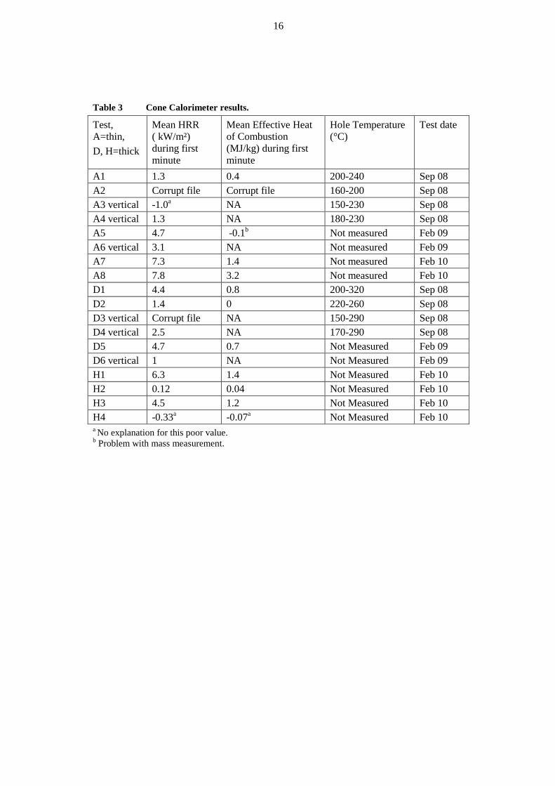
Figure 5 Results from TGA measurements. Other parameters needed are the HRR per Unit Area (HRRPUA) and the Heat of Combustion. Cone Calorimeter tests give a mean Heat Release Rate per Unit Area and an Effective Heat of Combustion as output. As the material disappeared early in the test, the time to hole opening was only about 10 s, the values for the first minute of the test was used. The results varied considerably as the mass loss rate from these thin membranes is very low and the mass loss is an important parameter in the calculation of Heat of Combustion. The results are presented in Table 3. Initially measurements were performed on membranes that had been tested in the SBI apparatus (membrane A and D). However, when the full scale validation experiments were planned, a new version of the thick membrane was provided and measurements were conducted on this membrane (membrane H) also. The poor outcome of many of the tests demonstrated the difficulties in obtaining correct data when the mass is as low as for the membrane. Also the process of opening up a hole is very quick, in the order of 10 seconds which increases the uncertainty even more. Please note that it is not possible to measure the Heat of Combustion in the vertical position as there is no mass loss scale in that position. Thermal properties of the membrane were assumed to correspond to soft PVC and were taken from literature: Cp = 0.88 kJ/kg.K, Conductivity = 0.19 W/mK 10.
0
50
100
150
200
250
300
350
50 52 54 56 58 60 62 64 66 68 70 72 74 76 78 80
Tem
pera
ture
°C
time, s
a2
T1
T2
Mass loss g/s thin material
-0.00001
0
0.00001
0.00002
0.00003
0.00004
0.00005
0 100 200 300 400 500 600
Temperature (°C)
mass loss g/s thick material
-0.00002
0
0.00002
0.00004
0.00006
0.00008
0.0001
0 100 200 300 400 500 600
Temperature °C
16
Table 3 Cone Calorimeter results.
Test, A=thin, D, H=thick
Mean HRR ( kW/m²) during first minute
Mean Effective Heat of Combustion (MJ/kg) during first minute
Hole Temperature (°C)
Test date
A1 1.3 0.4 200-240 Sep 08 A2 Corrupt file Corrupt file 160-200 Sep 08 A3 vertical -1.0a NA 150-230 Sep 08 A4 vertical 1.3 NA 180-230 Sep 08 A5 4.7 -0.1b Not measured Feb 09 A6 vertical 3.1 NA Not measured Feb 09 A7 7.3 1.4 Not measured Feb 10 A8 7.8 3.2 Not measured Feb 10 D1 4.4 0.8 200-320 Sep 08 D2 1.4 0 220-260 Sep 08 D3 vertical Corrupt file NA 150-290 Sep 08 D4 vertical 2.5 NA 170-290 Sep 08 D5 4.7 0.7 Not Measured Feb 09 D6 vertical 1 NA Not Measured Feb 09 H1 6.3 1.4 Not Measured Feb 10 H2 0.12 0.04 Not Measured Feb 10 H3 4.5 1.2 Not Measured Feb 10 H4 -0.33a -0.07a Not Measured Feb 10 a No explanation for this poor value. b Problem with mass measurement.
17
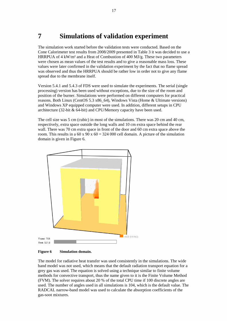
7 Simulations of validation experiment The simulation work started before the validation tests were conducted. Based on the Cone Calorimeter test results from 2008/2009 presented in Table 3 it was decided to use a HRRPUA of 4 kW/m² and a Heat of Combustion of 400 MJ/g. These two parameters were chosen as mean values of the test results and to give a reasonable mass loss. These values were later confirmed in the validation experiment by the fact that no flame spread was observed and thus the HRRPUA should be rather low in order not to give any flame spread due to the membrane itself. Version 5.4.1 and 5.4.3 of FDS were used to simulate the experiments. The serial (single processing) version has been used without exceptions, due to the size of the room and position of the burner. Simulations were performed on different computers for practical reasons. Both Linux (CentOS 5.3 x86_64), Windows Vista (Home & Ultimate versions) and Windows XP equipped computer were used. In addition, different setups in CPU architecture (32-bit & 64-bit) and CPU/Memory capacity have been used. The cell size was 5 cm (cubic) in most of the simulations. There was 20 cm and 40 cm, respectively, extra space outside the long walls and 10 cm extra space behind the rear wall. There was 70 cm extra space in front of the door and 60 cm extra space above the room. This results in a 60 x 90 x 60 = 324 000 cell domain. A picture of the simulation domain is given in Figure 6.
Figure 6 Simulation domain. The model for radiative heat transfer was used consistently in the simulations. The wide band model was not used, which means that the default radiation transport equation for a grey gas was used. The equation is solved using a technique similar to finite volume methods for convective transport, thus the name given to it is the Finite Volume Method (FVM). The solver requires about 20 % of the total CPU time if 100 discrete angles are used. The number of angles used in all simulations is 104, which is the default value. The RADCAL narrow-band model was used to calculate the absorption coefficients of the gas-soot mixtures.
18
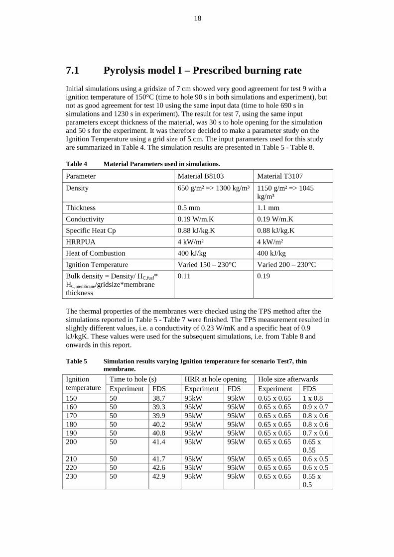
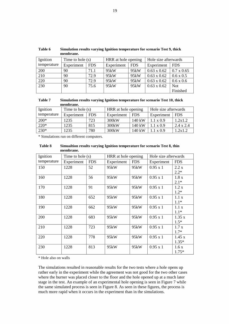
7.1 Pyrolysis model I – Prescribed burning rate Initial simulations using a gridsize of 7 cm showed very good agreement for test 9 with a ignition temperature of 150°C (time to hole 90 s in both simulations and experiment), but not as good agreement for test 10 using the same input data (time to hole 690 s in simulations and 1230 s in experiment). The result for test 7, using the same input parameters except thickness of the material, was 30 s to hole opening for the simulation and 50 s for the experiment. It was therefore decided to make a parameter study on the Ignition Temperature using a grid size of 5 cm. The input parameters used for this study are summarized in Table 4. The simulation results are presented in Table 5 - Table 8. Table 4 Material Parameters used in simulations.
Parameter Material B8103 Material T3107 Density 650 g/m² => 1300 kg/m³ 1150 g/m² => 1045
kg/m³ Thickness 0.5 mm 1.1 mm Conductivity 0.19 W/m.K 0.19 W/m.K Specific Heat Cp 0.88 kJ/kg.K 0.88 kJ/kg.K HRRPUA 4 kW/m² 4 kW/m² Heat of Combustion 400 kJ/kg 400 kJ/kg Ignition Temperature Varied 150 – 230°C Varied 200 – 230°C Bulk density = Density/ HC,fuel* HC,membrane/gridsize*membrane thickness
0.11 0.19
The thermal properties of the membranes were checked using the TPS method after the simulations reported in Table 5 - Table 7 were finished. The TPS measurement resulted in slightly different values, i.e. a conductivity of 0.23 W/mK and a specific heat of 0.9 kJ/kgK. These values were used for the subsequent simulations, i.e. from Table 8 and onwards in this report. Table 5 Simulation results varying Ignition temperature for scenario Test7, thin
membrane. Ignition temperature
Time to hole (s) HRR at hole opening Hole size afterwards Experiment FDS Experiment FDS Experiment FDS
150 50 38.7 95kW 95kW 0.65 x 0.65 1 x 0.8 160 50 39.3 95kW 95kW 0.65 x 0.65 0.9 x 0.7 170 50 39.9 95kW 95kW 0.65 x 0.65 0.8 x 0.6 180 50 40.2 95kW 95kW 0.65 x 0.65 0.8 x 0.6 190 50 40.8 95kW 95kW 0.65 x 0.65 0.7 x 0.6 200 50 41.4 95kW 95kW 0.65 x 0.65 0.65 x
0.55 210 50 41.7 95kW 95kW 0.65 x 0.65 0.6 x 0.5 220 50 42.6 95kW 95kW 0.65 x 0.65 0.6 x 0.5 230 50 42.9 95kW 95kW 0.65 x 0.65 0.55 x
0.5
19
Table 6 Simulation results varying Ignition temperature for scenario Test 9, thick
membrane. Ignition temperature
Time to hole (s) HRR at hole opening Hole size afterwards Experiment FDS Experiment FDS Experiment FDS
200 90 71.1 95kW 95kW 0.63 x 0.62 0.7 x 0.65 210 90 72.9 95kW 95kW 0.63 x 0.62 0.6 x 0.5 220 90 72.9 95kW 95kW 0.63 x 0.62 0.6 x 0.6 230 90 75.6 95kW 95kW 0.63 x 0.62 Not
Finished Table 7 Simulation results varying Ignition temperature for scenario Test 10, thick
membrane. Ignition temperature
Time to hole (s) HRR at hole opening Hole size afterwards Experiment FDS Experiment FDS Experiment FDS
200* 1235 723 300kW 140 kW 1.1 x 0.9 1.2x1.2 220* 1235 815 300kW 140 kW 1.1 x 0.9 2.4 x 2.4 230* 1235 780 300kW 140 kW 1.1 x 0.9 1.2x1.2 * Simulations run on different computers. Table 8 Simualtion results varying Ignition temperature for scenario Test 8, thin
membrane. Ignition temperature
Time to hole (s) HRR at hole opening Hole size afterwards Experiment FDS Experiment FDS Experiment FDS
150 1228 52 95kW 95kW 0.95 x 1 2.2 x 2.2*
160 1228 56 95kW 95kW 0.95 x 1 1.8 x 2.1*
170 1228 91 95kW 95kW 0.95 x 1 1.2 x 1.2*
180 1228 652 95kW 95kW 0.95 x 1 1.1 x 1.1*
190 1228 662 95kW 95kW 0.95 x 1 1.1 x 1.1*
200 1228 683 95kW 95kW 0.95 x 1 1.35 x 1.5*
210 1228 723 95kW 95kW 0.95 x 1 1.7 x 1.7*
220 1228 778 95kW 95kW 0.95 x 1 1.45 x 1.35*
230 1228 813 95kW 95kW 0.95 x 1 1.6 x 1.75*
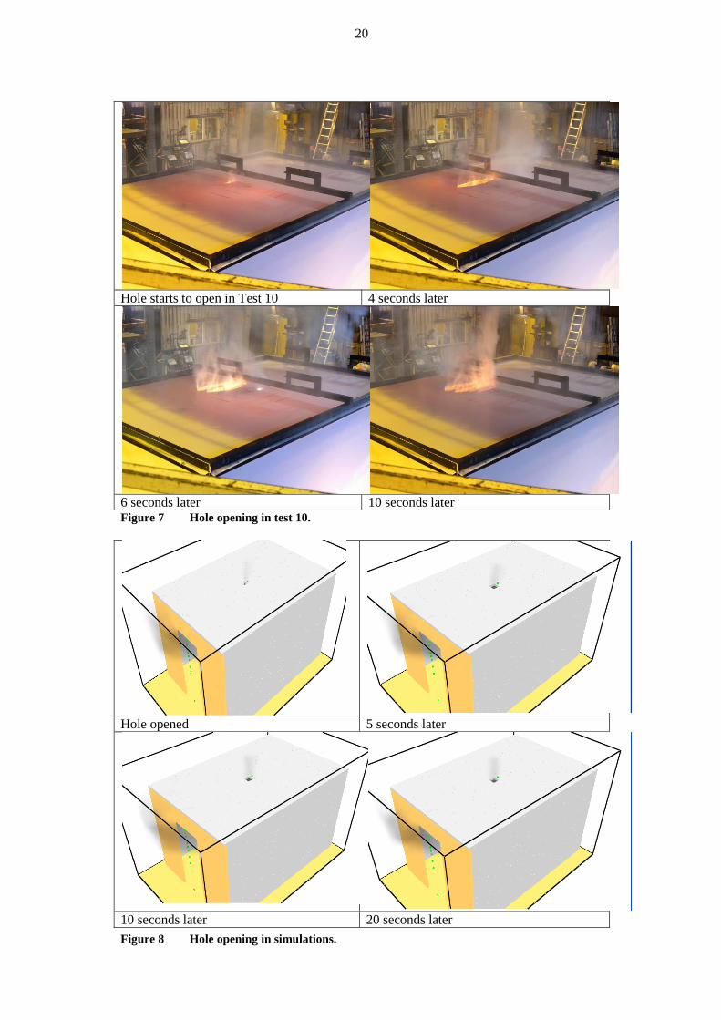
* Hole also on walls The simulations resulted in reasonable results for the two tests where a hole opens up rather early in the experiment while the agreement was not good for the two other cases where the burner was placed closer to the floor and the hole opened up at a much later stage in the test. An example of an experimental hole opening is seen in Figure 7 while the same simulated process is seen in Figure 8. As seen in these figures, the process is much more rapid when it occurs in the experiment than in the simulations.
20
Hole starts to open in Test 10 4 seconds later
6 seconds later 10 seconds later Figure 7 Hole opening in test 10.
Hole opened 5 seconds later
10 seconds later 20 seconds later Figure 8 Hole opening in simulations.
21
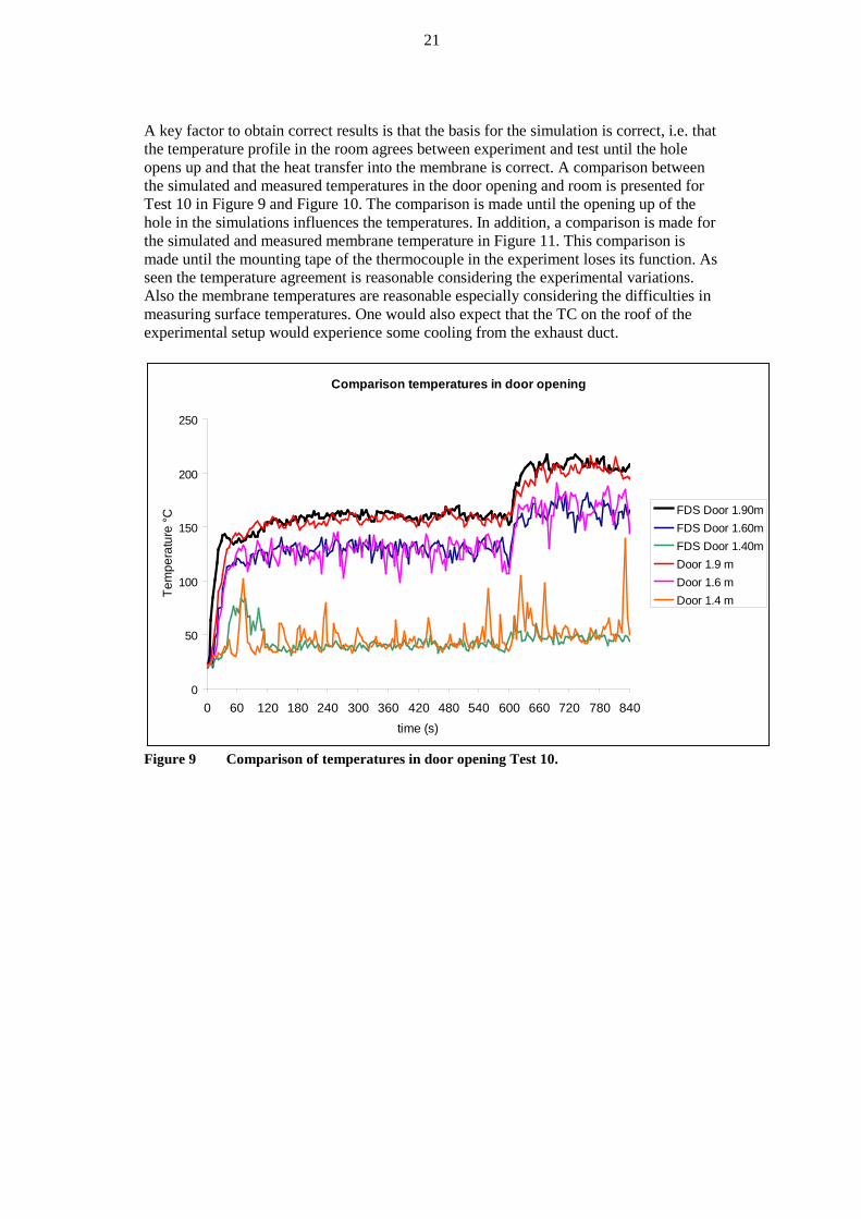
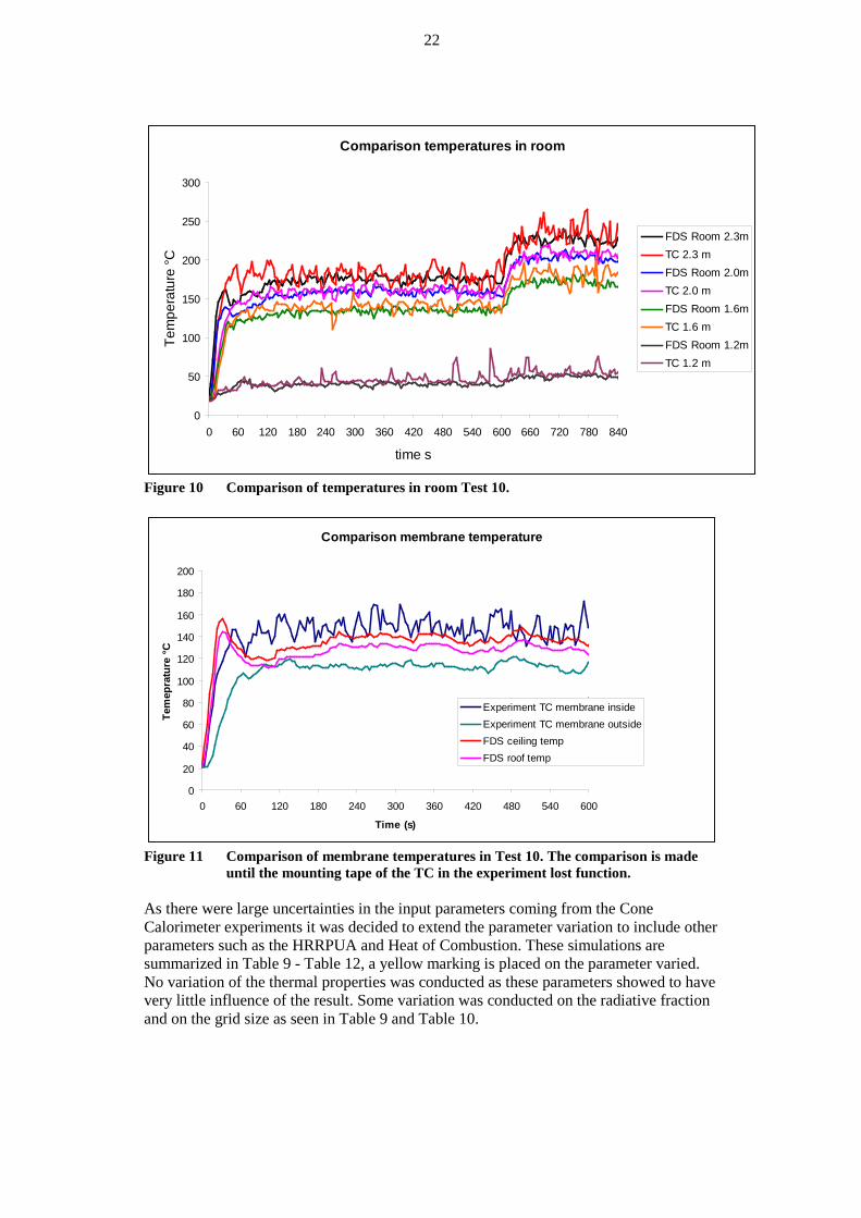
A key factor to obtain correct results is that the basis for the simulation is correct, i.e. that the temperature profile in the room agrees between experiment and test until the hole opens up and that the heat transfer into the membrane is correct. A comparison between the simulated and measured temperatures in the door opening and room is presented for Test 10 in Figure 9 and Figure 10. The comparison is made until the opening up of the hole in the simulations influences the temperatures. In addition, a comparison is made for the simulated and measured membrane temperature in Figure 11. This comparison is made until the mounting tape of the thermocouple in the experiment loses its function. As seen the temperature agreement is reasonable considering the experimental variations. Also the membrane temperatures are reasonable especially considering the difficulties in measuring surface temperatures. One would also expect that the TC on the roof of the experimental setup would experience some cooling from the exhaust duct.
Figure 9 Comparison of temperatures in door opening Test 10.
Comparison temperatures in door opening
0
50
100
150
200
250
0 60 120 180 240 300 360 420 480 540 600 660 720 780 840time (s)
Tem
pera
ture
°C
FDS Door 1.90mFDS Door 1.60mFDS Door 1.40mDoor 1.9 mDoor 1.6 mDoor 1.4 m
22
Figure 10 Comparison of temperatures in room Test 10.
Figure 11 Comparison of membrane temperatures in Test 10. The comparison is made
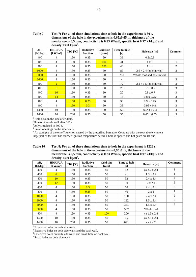
until the mounting tape of the TC in the experiment lost function. As there were large uncertainties in the input parameters coming from the Cone Calorimeter experiments it was decided to extend the parameter variation to include other parameters such as the HRRPUA and Heat of Combustion. These simulations are summarized in Table 9 - Table 12, a yellow marking is placed on the parameter varied. No variation of the thermal properties was conducted as these parameters showed to have very little influence of the result. Some variation was conducted on the radiative fraction and on the grid size as seen in Table 9 and Table 10.
Comparison temperatures in room
0
50
100
150
200
250
300
0 60 120 180 240 300 360 420 480 540 600 660 720 780 840
time s
Tem
pera
ture
°C
FDS Room 2.3mTC 2.3 mFDS Room 2.0mTC 2.0 mFDS Room 1.6mTC 1.6 mFDS Room 1.2mTC 1.2 m
Comparison membrane temperature
0
20
40
60
80
100
120
140
160
180
200
0 60 120 180 240 300 360 420 480 540 600
Time (s)
Tem
epra
ture
°C
Experiment TC membrane insideExperiment TC membrane outsideFDS ceiling tempFDS roof temp
23
Table 9 Test 7; For all of these simulations time to hole in the experiment is 50 s,
dimensions of the hole in the experiments is 0,65x0,65 m, thickness of the membrane is 0,5 mm, conductivity is 0.23 W/mK, specific heat 0.97 kJ/kgK and density 1300 kg/m3.
ΔHc [kJ/kg]
HRRPUA [kW/m²] TIG [ºC] Radiative
fraction Grid size
[mm] Time to hole
[s] Hole size [m] Comment
400 4 150 0.35 50 39 0.8x0.8 400 4 150 0.35 100 41 1 x 1 1
400 4 150 0.35 150 46 1 x 1 2 1000 4 150 0.35 50 89 2.6 x 2.4 (hole in wall) 3 3000 4 150 0.35 50 250 Whole roof and hole in wall
6000 4 150 0.35 50 -
3 400 2 150 0.35 50 72 2.1 x 1.5 (hole in wall) 3 400 6 150 0.35 50 28 0.9 x 0.7 3 400 10 150 0.35 50 20 0.8 x 0.7 3 400 14 150 0.35 50 16 0.8 x 0.75 3 400 4 150 0.25 50 38 0.9 x 0.75 3 400 4 150 0.3 50 38 0.95 x 0.8 3
1400 10 150 0.35 50 52 ca 2.4 x 2.4 4 1400 10 200 0.35 50 55 0.65 x 0.55 5
1 Hole also on the side after 410s. 2Hole on the side wall after 360 s. 3Only simulated to 500 s. 4 Small openings on the side walls. 5 An example of the on/off function caused by the prescribed burn rate. Compare with the row above where a large part of the roof has reached ignition temperature before a hole is opened and hot gases are let out. Table 10 Test 8; For all of these simulations time to hole in the experiment is 1228 s,
dimensions of the hole in the experiments is 0,95x1 m, thickness of the membrane is 0,5 mm, conductivity is 0.23 W/mK, specific heat 0.97 kJ/kgK and density 1300 kg/m3.
ΔHc [kJ/kg]
HRRPUA [kW/m²] TIG [ºC] Radiative
fraction Grid size
[mm] Time to hole
[s] Hole size [m] Comment
400 4 150 0.35 50 52 ca 2.2 x 2.4 1 400 6 150 0.35 50 41 1.3 x 2.4 1 400 10 150 0.35 50 32 2.4 x 2.4 2 400 12 150 0.35 50 30 2 x 2.4 2 400 4 150 0.3 50 50 2.4 x 2.4 3 400 4 150 0.25 50 46 2 x 2 1
1000 4 150 0.35 50 100 2.4 x 2.4 2 2000 4 150 0.35 50 182 1.5 x 2.4 2 4000 4 150 0.35 50 344 1.5 x 1.8 4 6000 4 150 0.35 50 507 Whole roof 400 4 150 0.35 100 206 ca 1.6 x 2.4
1400 10 150 0.35 50 65 ca 2.5 x 2.4 1400 10 200 0.35 50 691 ca 2 x 2
1 Extensive holes on both side walls. 2 Extensive holes on both side walls and the back wall. 3 Extensive holes on both side walls and small hole on back wall. 4 Small holes on both side walls.
24
Table 11 Test 9; For all of these simulations time to hole in the experiment is 90 s,
dimensions of the hole in the experiments is 0,63x0,62 m, thickness of the membrane is 1,1 mm, conductivity is 0.23 W/mK, specific heat 0.97 kJ/kgK and density 1045 kg/m3.
ΔHc [kJ/kg]
HRRPUA [kW/m²] TIG [ºC] Radiative
fraction Grid size [mm] Time to hole [s] Hole size [m] Comment
2100 10 150 0.35 50 131 The whole roof 1 2100 10 200 0.35 50 135 0.65 x 0.55
1 Hole on large parts of the side walls. Table 12 Test 10; For all of these simulations time to hole in the experiment is 1235 s,
dimensions of the hole in the experiments is 1,11 x 0,9 m, thickness of the membrane is 1,1 mm, conductivity is 0.23 W/mK, specific heat 0.97 kJ/kgK and density 1045 kg/m3.
ΔHc [kJ/kg]
HRRPUA [kW/m²] TIG [ºC] Radiative
fraction Grid size
[mm] Time to hole
[s] Hole size [m] Comment
2100 10 150 0.35 50 409 ca 2.4 x 2.4 1 2100 10 200 0.35 50 756 The whole roof 2
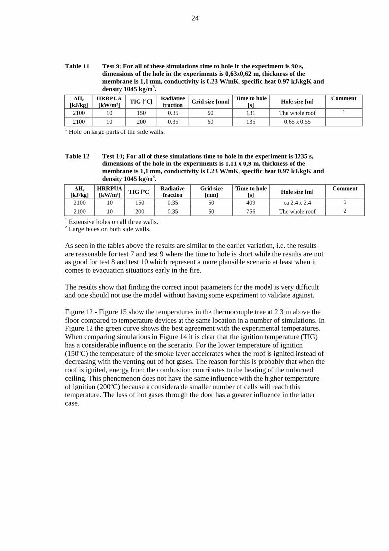
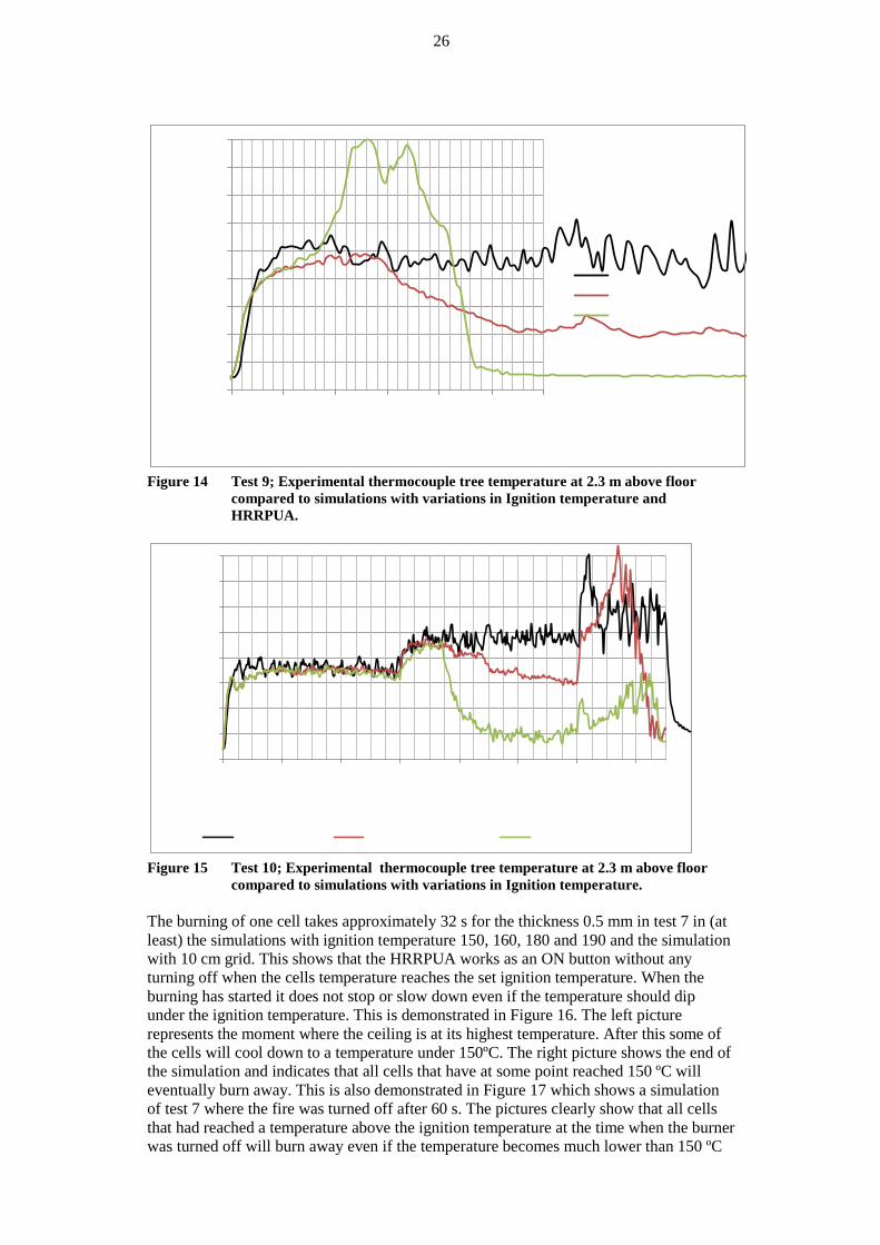
1 Extensive holes on all three walls. 2 Large holes on both side walls. As seen in the tables above the results are similar to the earlier variation, i.e. the results are reasonable for test 7 and test 9 where the time to hole is short while the results are not as good for test 8 and test 10 which represent a more plausible scenario at least when it comes to evacuation situations early in the fire. The results show that finding the correct input parameters for the model is very difficult and one should not use the model without having some experiment to validate against. Figure 12 - Figure 15 show the temperatures in the thermocouple tree at 2.3 m above the floor compared to temperature devices at the same location in a number of simulations. In Figure 12 the green curve shows the best agreement with the experimental temperatures. When comparing simulations in Figure 14 it is clear that the ignition temperature (TIG) has a considerable influence on the scenario. For the lower temperature of ignition (150ºC) the temperature of the smoke layer accelerates when the roof is ignited instead of decreasing with the venting out of hot gases. The reason for this is probably that when the roof is ignited, energy from the combustion contributes to the heating of the unburned ceiling. This phenomenon does not have the same influence with the higher temperature of ignition (200ºC) because a considerable smaller number of cells will reach this temperature. The loss of hot gases through the door has a greater influence in the latter case.
25
Figure 12 Test 7; Experimental thermocouple tree temperature at 2.3 m above floor
compared to simulations with variations in Ignition temperature, ΔHc and HRRPUA.
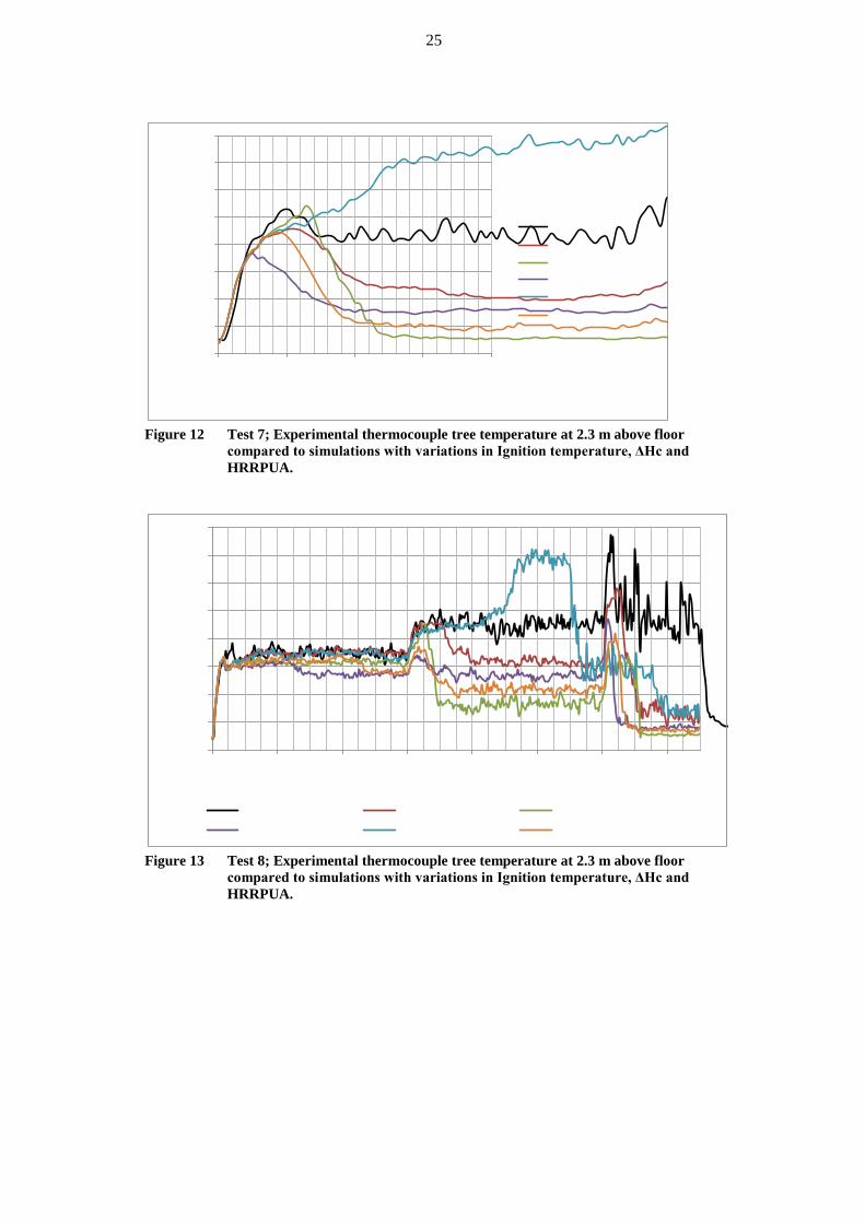
Figure 13 Test 8; Experimental thermocouple tree temperature at 2.3 m above floor
compared to simulations with variations in Ignition temperature, ΔHc and HRRPUA.
0
50
100
150
200
250
300
350
400
0 50 100 150 200
Tem
pera
ture
, TC
230c
m [º
C]
Time [s]
Experiment, test 7
Tig200_dhc1400_HRRPUA10
Tig150_dhc1400_HRRPUA10
Tig150_dhc400_HRRPUA10
Tig150_dhc6000_HRRPUA4
Tig150_dhc400_HRRPUA4
0
50
100
150
200
250
300
350
400
0 200 400 600 800 1000 1200 1400
Tem
pera
ture
, TC
230c
m [º
C]
Time [s]Experiment, test 8 Tig200_dhc1400_HRRPUA10 Tig150_dhc1400_HRRPUA10
Tig150_dhc400_HRRPUA10 Tig150_dhc6000_HRRPUA4 Tig150_dhc400_HRRPUA4
26
Figure 14 Test 9; Experimental thermocouple tree temperature at 2.3 m above floor
compared to simulations with variations in Ignition temperature and HRRPUA.
Figure 15 Test 10; Experimental thermocouple tree temperature at 2.3 m above floor
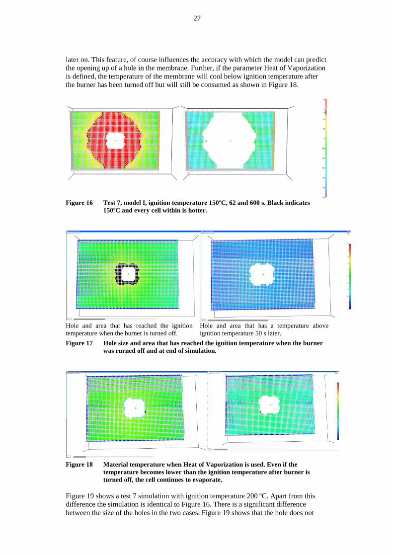
compared to simulations with variations in Ignition temperature. The burning of one cell takes approximately 32 s for the thickness 0.5 mm in test 7 in (at least) the simulations with ignition temperature 150, 160, 180 and 190 and the simulation with 10 cm grid. This shows that the HRRPUA works as an ON button without any turning off when the cells temperature reaches the set ignition temperature. When the burning has started it does not stop or slow down even if the temperature should dip under the ignition temperature. This is demonstrated in Figure 16. The left picture represents the moment where the ceiling is at its highest temperature. After this some of the cells will cool down to a temperature under 150ºC. The right picture shows the end of the simulation and indicates that all cells that have at some point reached 150 ºC will eventually burn away. This is also demonstrated in Figure 17 which shows a simulation of test 7 where the fire was turned off after 60 s. The pictures clearly show that all cells that had reached a temperature above the ignition temperature at the time when the burner was turned off will burn away even if the temperature becomes much lower than 150 ºC
0
50
100
150
200
250
300
350
400
450
0 50 100 150 200 250 300
Tem
pera
ture
, TC2
30cm
[ºC]
Time [s]
Experiment, test 9
Tig200_dhc2100_HRRPUA10
Tig150_dhc2100_HRRPUA10
0
50
100
150
200
250
300
350
400
0 200 400 600 800 1000 1200 1400
Tem
pera
ture
, TC2
30cm
[ºC
]
Time [s]
Experiment, test 10 Tig200_dhc2100_HRRPUA10 Tig150_dhc2100_HRRPUA10
27
later on. This feature, of course influences the accuracy with which the model can predict the opening up of a hole in the membrane. Further, if the parameter Heat of Vaporization is defined, the temperature of the membrane will cool below ignition temperature after the burner has been turned off but will still be consumed as shown in Figure 18.
Figure 16 Test 7, model I, ignition temperature 150ºC, 62 and 600 s. Black indicates
150ºC and every cell within is hotter.
Hole and area that has reached the ignition temperature when the burner is turned off.
Hole and area that has a temperature above ignition temperature 50 s later.
Figure 17 Hole size and area that has reached the ignition temperature when the burner was rurned off and at end of simulation.
Figure 18 Material temperature when Heat of Vaporization is used. Even if the temperature becomes lower than the ignition temperature after burner is turned off, the cell continues to evaporate.
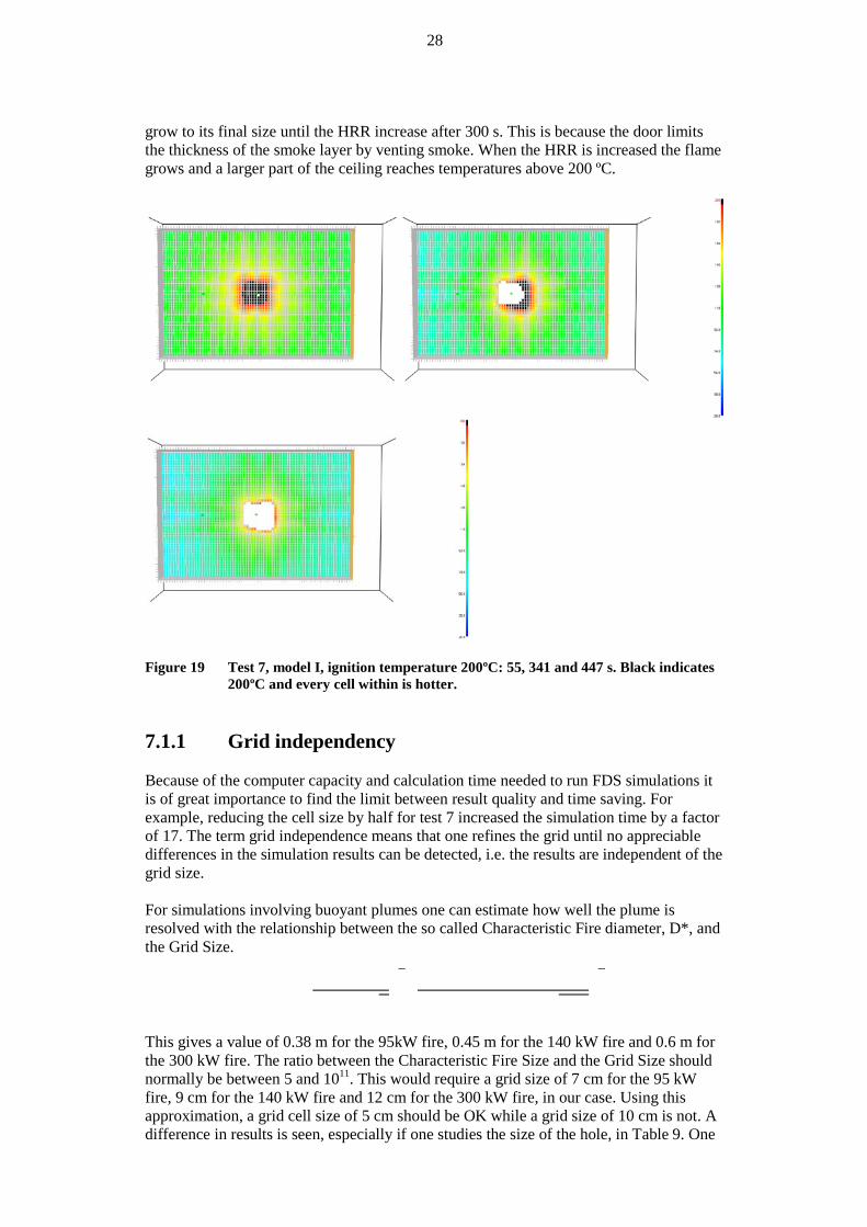
Figure 19 shows a test 7 simulation with ignition temperature 200 ºC. Apart from this difference the simulation is identical to Figure 16. There is a significant difference between the size of the holes in the two cases. Figure 19 shows that the hole does not
28
grow to its final size until the HRR increase after 300 s. This is because the door limits the thickness of the smoke layer by venting smoke. When the HRR is increased the flame grows and a larger part of the ceiling reaches temperatures above 200 ºC.
Figure 19 Test 7, model I, ignition temperature 200ºC: 55, 341 and 447 s. Black indicates
200ºC and every cell within is hotter. 7.1.1 Grid independency Because of the computer capacity and calculation time needed to run FDS simulations it is of great importance to find the limit between result quality and time saving. For example, reducing the cell size by half for test 7 increased the simulation time by a factor of 17. The term grid independence means that one refines the grid until no appreciable differences in the simulation results can be detected, i.e. the results are independent of the grid size. For simulations involving buoyant plumes one can estimate how well the plume is resolved with the relationship between the so called Characteristic Fire diameter, D*, and the Grid Size.
This gives a value of 0.38 m for the 95kW fire, 0.45 m for the 140 kW fire and 0.6 m for the 300 kW fire. The ratio between the Characteristic Fire Size and the Grid Size should normally be between 5 and 1011. This would require a grid size of 7 cm for the 95 kW fire, 9 cm for the 140 kW fire and 12 cm for the 300 kW fire, in our case. Using this approximation, a grid cell size of 5 cm should be OK while a grid size of 10 cm is not. A difference in results is seen, especially if one studies the size of the hole, in Table 9. One
29
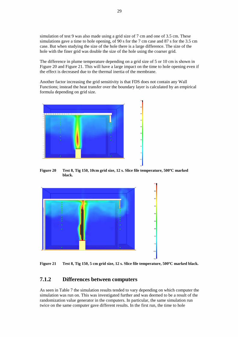
simulation of test 9 was also made using a grid size of 7 cm and one of 3.5 cm. These simulations gave a time to hole opening, of 90 s for the 7 cm case and 87 s for the 3.5 cm case. But when studying the size of the hole there is a large difference. The size of the hole with the finer grid was double the size of the hole using the coarser grid. The difference in plume temperature depending on a grid size of 5 or 10 cm is shown in Figure 20 and Figure 21. This will have a large impact on the time to hole opening even if the effect is decreased due to the thermal inertia of the membrane. Another factor increasing the grid sensitivity is that FDS does not contain any Wall Functions; instead the heat transfer over the boundary layer is calculated by an empirical formula depending on grid size.
Figure 20 Test 8, Tig 150, 10cm grid size, 12 s. Slice file temperature, 500ºC marked
black.
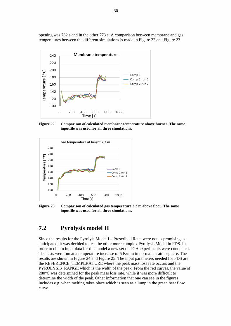
Figure 21 Test 8, Tig 150, 5 cm grid size, 12 s. Slice file temperature, 500ºC marked black. 7.1.2 Differences between computers As seen in Table 7 the simulation results tended to vary depending on which computer the simulation was run on. This was investigated further and was deemed to be a result of the randomization value generator in the computers. In particular, the same simulation run twice on the same computer gave different results. In the first run, the time to hole
30
opening was 762 s and in the other 773 s. A comparison between membrane and gas temperatures between the different simulations is made in Figure 22 and Figure 23.
Figure 22 Comparison of calculated membrane temperature above burner. The same
inputfile was used for all three simulations.
Figure 23 Comparison of calculated gas temperature 2.2 m above floor. The same
inputfile was used for all three simulations.
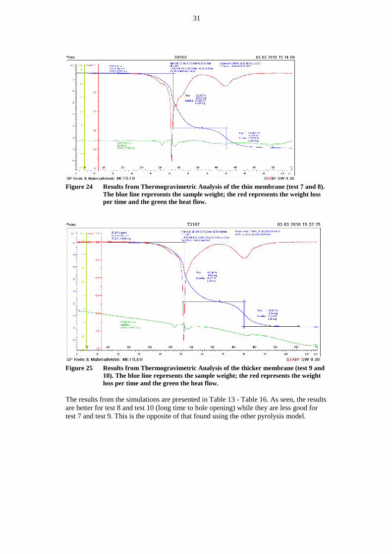
7.2 Pyrolysis model II Since the results for the Pyrolyis Model I – Prescribed Rate, were not as promising as anticipated, it was decided to test the other more complex Pyrolysis Model in FDS. In order to obtain input data for this model a new set of TGA experiments were conducted. The tests were run at a temperature increase of 5 K/min in normal air atmosphere. The results are shown in Figure 24 and Figure 25. The input parameters needed for FDS are the REFERENCE_TEMPERATURE where the peak mass loss rate occurs and the PYROLYSIS_RANGE which is the width of the peak. From the red curves, the value of 280°C was determined for the peak mass loss rate, while it was more difficult to determine the width of the peak. Other information that one can see in the figures includes e.g. when melting takes place which is seen as a lump in the green heat flow curve.
31
Figure 24 Results from Thermogravimetric Analysis of the thin membrane (test 7 and 8).
The blue line represents the sample weight; the red represents the weight loss per time and the green the heat flow.
Figure 25 Results from Thermogravimetric Analysis of the thicker membrane (test 9 and
10). The blue line represents the sample weight; the red represents the weight loss per time and the green the heat flow.
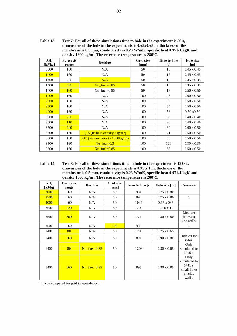
The results from the simulations are presented in Table 13 - Table 16. As seen, the results are better for test 8 and test 10 (long time to hole opening) while they are less good for test 7 and test 9. This is the opposite of that found using the other pyrolysis model.
32
Table 13 Test 7; For all of these simulations time to hole in the experiment is 50 s,
dimensions of the hole in the experiments is 0.65x0.65 m, thickness of the membrane is 0.5 mm, conductivity is 0.23 W/mK, specific heat 0.97 kJ/kgK and density 1300 kg/m3. The reference temperature is 280ºC.
ΔHc [kJ/kg]
Pyrolysis range Residue Grid size
[mm] Time to hole
[s] Hole size
[m] 3500 160 N/A 50 18 0.45 x 0.45 1400 160 N/A 50 17 0.45 x 0.45 1400 80 N/A 50 16 0.35 x 0.35 1400 80 Nu_fuel=0,85 50 16 0.35 x 0.35 1400 160 Nu_fuel=0,85 50 18 0.50 x 0.50 1000 160 N/A 100 28 0.60 x 0.50 2000 160 N/A 100 36 0.50 x 0.50 3500 160 N/A 100 54 0.50 x 0.50 4000 160 N/A 100 58 0.50 x0.50 3500 80 N/A 100 28 0.40 x 0.40 3500 110 N/A 100 30 0.40 x 0.40 3500 240 N/A 100 69 0.60 x 0.50 3500 160 0,15 (residue density 5kg/m³) 100 71 0.50 x 0.50 3500 160 0,15 (residue density 1300kg/m³) 100 66 0.50 x 0.50 3500 160 Nu_fuel=0,3 100 121 0.30 x 0.30 3500 160 Nu_fuel=0,85 100 68 0.50 x 0.50
Table 14 Test 8; For all of these simulations time to hole in the experiment is 1228 s,
dimensions of the hole in the experiments is 0.95 x 1 m, thickness of the membrane is 0.5 mm, conductivity is 0.23 W/mK, specific heat 0.97 kJ/kgK and density 1300 kg/m3. The reference temperature is 280ºC.
ΔHc [kJ/kg
Pyrolysis range Residue Grid size
[mm] Time to hole [s] Hole size [m] Comment
3000 160 N/A 50 984 0.75 x 0.80 3500 160 N/A 50 997 0.75 x 0.80 1 4000 160 N/A 50 1044 0.75 x 085 3500 120 N/A 50 1209 0.90 x 1
3500 200 N/A 50 774 0.80 x 0.80 Medium holes on
side walls. 3500 160 N/A 100 985 1 1400 80 N/A 50 1205 0.75 x 0.65
1400 160 N/A 50 801 0.90 x 0.80 Hole on the sides.
1400 80 Nu_fuel=0.85 50 1206 0.80 x 0.65 Only
simulated to 1419 s.
1400 160 Nu_fuel=0.85 50 895 0.80 x 0.85
Only simulated to
1441 s. Small holes
on side walls.
1 To be compared for grid independency.
33
Table 15 Test 9; For all of these simulations time to hole in the experiment is 90 s,
dimensions of the hole in the experiments is 0.63 x 0.62 m, thickness of the membrane is 1.1 mm, conductivity is 0.23 W/mK, specific heat 0.97 kJ/kgK and density 1045 kg/m3. The reference temperature is 280ºC.
ΔHc [kJ/kg] Pyrolysis range Residue Grid size [mm] Time to hole [s] Hole size [m] 2100 80 N/A 50 24 0.40 x 0.40 2100 160 N/A 50 29 0.50 x 0.50 2100 80 Nu_fuel=0.85 50 25 0.35 x 0.40 2100 160 Nu_fuel=0.85 50 31 0.50 x 0.50
Table 16 Test 10; For all of these simulations time to hole in the experiment is 1228 s,
dimensions of the hole in the experiments is 1.1 x 0.9 m, thickness of the membrane is 1,1 mm, conductivity is 0.23 W/mK, specific heat 0.97 kJ/kgK and density 1045 kg/m3. The reference temperature is 280ºC.
ΔHc [kJ/kg]
Pyrolysis range Residue Grid size
[mm] Time to hole
[s] Hole size
[m] Comment
2100 80 N/A 50 1206 1 x 0.9 2100 160 N/A 50 700 0.9 x 0.85 Large holes on side walls. 2100 80 Nu_fuel=0.85 50 1206 0.95 x 0.85 Only simulated to 1317 s.
2100 160 Nu_fuel=0.85 50 873 0.8 x 0.75 Only simulated to 1405,5 s. Holes on side walls.
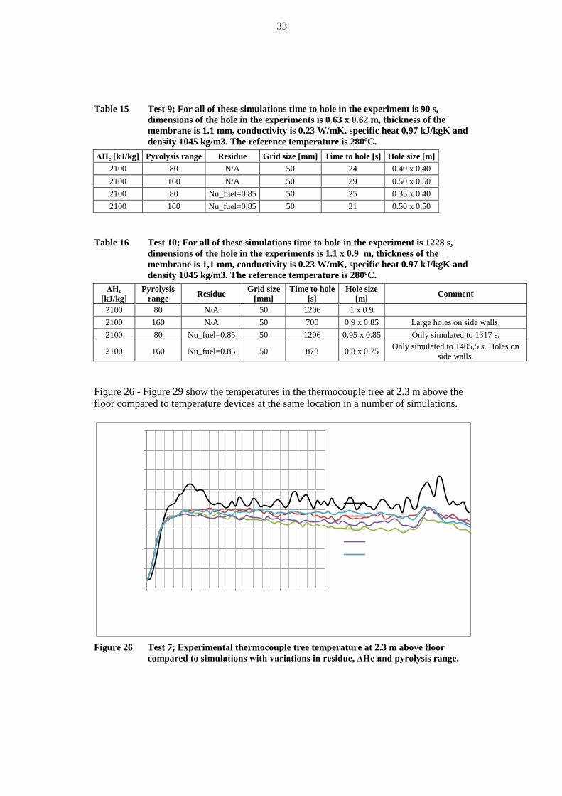
Figure 26 - Figure 29 show the temperatures in the thermocouple tree at 2.3 m above the floor compared to temperature devices at the same location in a number of simulations.
Figure 26 Test 7; Experimental thermocouple tree temperature at 2.3 m above floor
compared to simulations with variations in residue, ΔHc and pyrolysis range.
0
50
100
150
200
250
300
350
400
0 50 100 150 200
Tem
pera
ture
, TC2
30cm
[ºC]
Time [s]
Experiment, test 7
PyrolysisRange80_dhc1400
PyrolysisRange160_dhc1400
PyrolysisRange160_dhc3500
PyrolysisRange80_dhc1400_residue
34
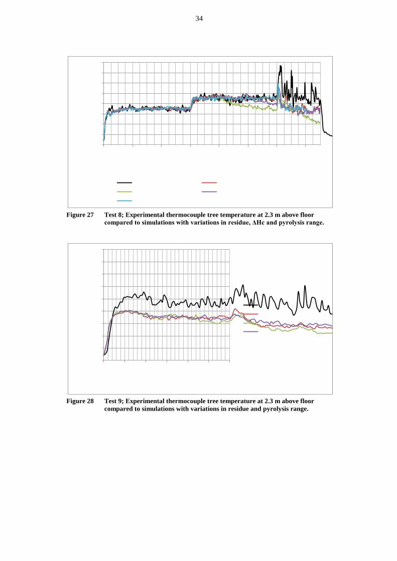
Figure 27 Test 8; Experimental thermocouple tree temperature at 2.3 m above floor
compared to simulations with variations in residue, ΔHc and pyrolysis range.
Figure 28 Test 9; Experimental thermocouple tree temperature at 2.3 m above floor
compared to simulations with variations in residue and pyrolysis range.
0
50
100
150
200
250
300
350
400
0 200 400 600 800 1000 1200 1400Tem
pera
ture
, TC2
30cm
[ºC]
Time [s]
Experiment, test 8 PyrolysisRange80_dhc1400
PyrolysisRange160_dhc1400 PyrolysisRange160_dhc3500
PyrolysisRange80_dhc1400_residue
0
50
100
150
200
250
300
350
400
450
0 50 100 150 200 250 300
Tem
pera
ture
, TC2
30cm
[ºC]
Time [s]
Experiment, test 9
PyrolysisRange80_dhc2100
PyrolysisRange160_dhc2100
PyrolysisRange80_dhc2100_residue
35
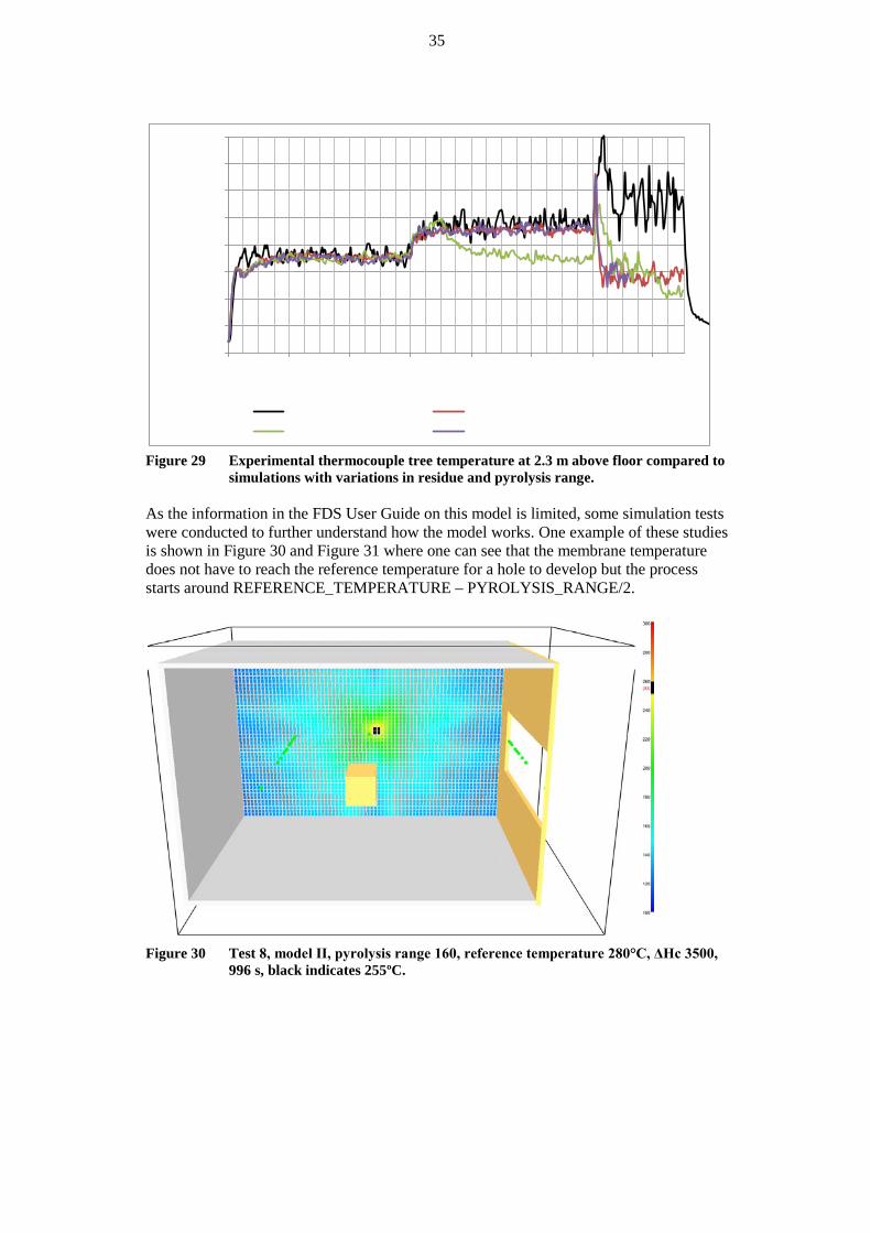
Figure 29 Experimental thermocouple tree temperature at 2.3 m above floor compared to
simulations with variations in residue and pyrolysis range. As the information in the FDS User Guide on this model is limited, some simulation tests were conducted to further understand how the model works. One example of these studies is shown in Figure 30 and Figure 31 where one can see that the membrane temperature does not have to reach the reference temperature for a hole to develop but the process starts around REFERENCE_TEMPERATURE – PYROLYSIS_RANGE/2.
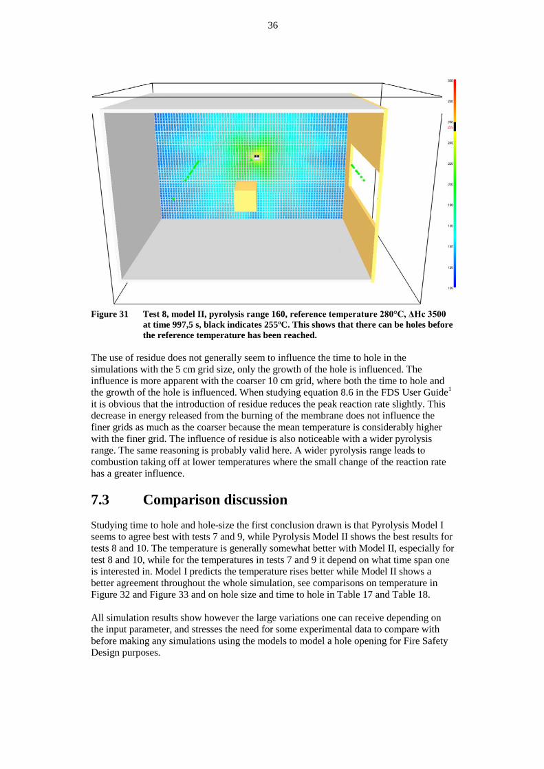
Figure 30 Test 8, model II, pyrolysis range 160, reference temperature 280°C, ΔHc 3500,
996 s, black indicates 255ºC.
0
50
100
150
200
250
300
350
400
0 200 400 600 800 1000 1200 1400
Tem
pera
ture
, TC2
30cm
[ºC]
Time [s]Experiment, test 10 PyrolysisRange80_dhc2100
PyrolysisRange160_dhc2100 PyrolysisRange80_dhc2100_residue
36
Figure 31 Test 8, model II, pyrolysis range 160, reference temperature 280°C, ΔHc 3500
at time 997,5 s, black indicates 255ºC. This shows that there can be holes before the reference temperature has been reached.
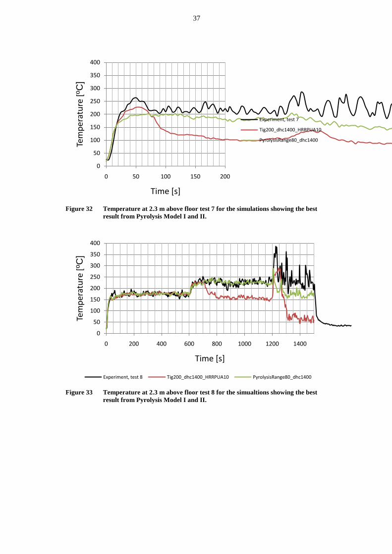
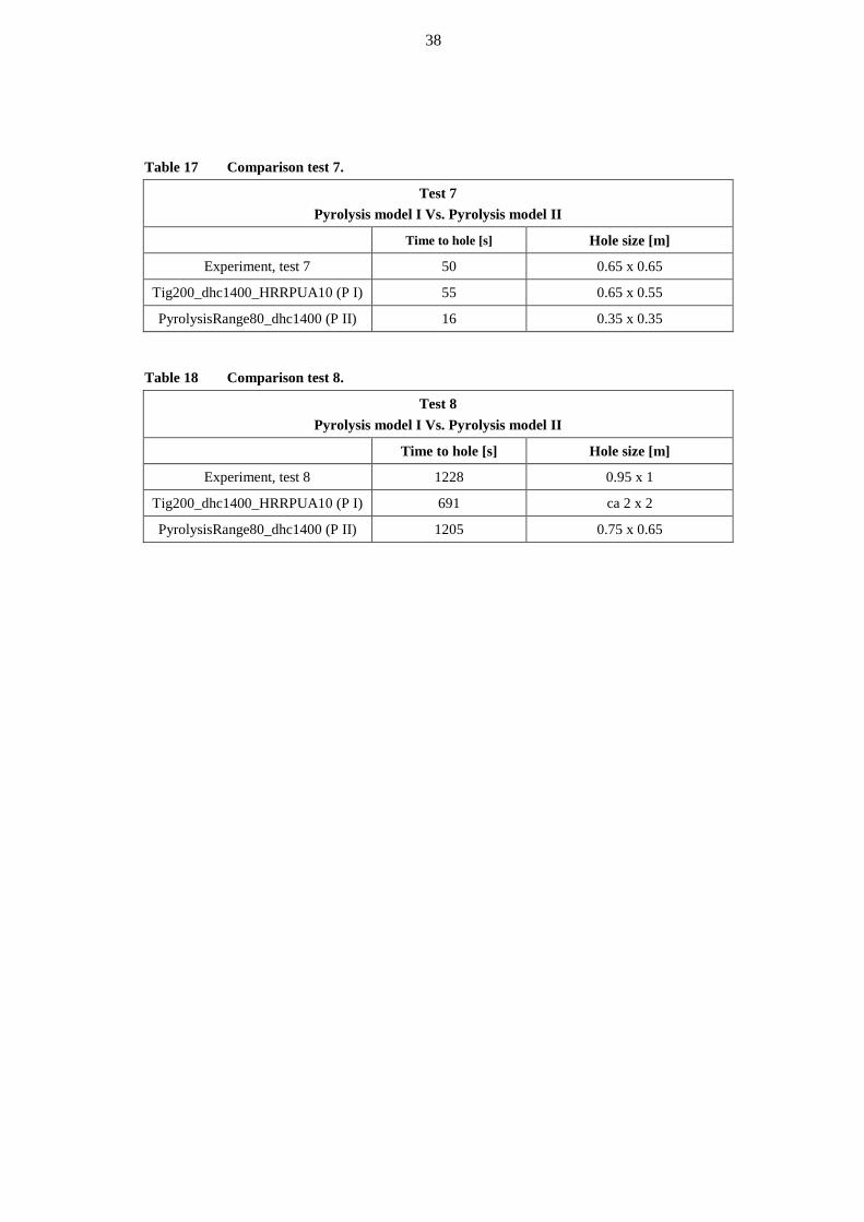
The use of residue does not generally seem to influence the time to hole in the simulations with the 5 cm grid size, only the growth of the hole is influenced. The influence is more apparent with the coarser 10 cm grid, where both the time to hole and the growth of the hole is influenced. When studying equation 8.6 in the FDS User Guide1 it is obvious that the introduction of residue reduces the peak reaction rate slightly. This decrease in energy released from the burning of the membrane does not influence the finer grids as much as the coarser because the mean temperature is considerably higher with the finer grid. The influence of residue is also noticeable with a wider pyrolysis range. The same reasoning is probably valid here. A wider pyrolysis range leads to combustion taking off at lower temperatures where the small change of the reaction rate has a greater influence. 7.3 Comparison discussion Studying time to hole and hole-size the first conclusion drawn is that Pyrolysis Model I seems to agree best with tests 7 and 9, while Pyrolysis Model II shows the best results for tests 8 and 10. The temperature is generally somewhat better with Model II, especially for test 8 and 10, while for the temperatures in tests 7 and 9 it depend on what time span one is interested in. Model I predicts the temperature rises better while Model II shows a better agreement throughout the whole simulation, see comparisons on temperature in Figure 32 and Figure 33 and on hole size and time to hole in Table 17 and Table 18. All simulation results show however the large variations one can receive depending on the input parameter, and stresses the need for some experimental data to compare with before making any simulations using the models to model a hole opening for Fire Safety Design purposes.
37
Figure 32 Temperature at 2.3 m above floor test 7 for the simulations showing the best
result from Pyrolysis Model I and II.
Figure 33 Temperature at 2.3 m above floor test 8 for the simualtions showing the best
result from Pyrolysis Model I and II.
0
50
100
150
200
250
300
350
400
0 50 100 150 200
Tem
pera
ture
[ºC
]
Time [s]
Experiment, test 7
Tig200_dhc1400_HRRPUA10
PyrolysisRange80_dhc1400
0
50
100
150
200
250
300
350
400
0 200 400 600 800 1000 1200 1400
Tem
pera
ture
[ºC
]
Time [s]
Experiment, test 8 Tig200_dhc1400_HRRPUA10 PyrolysisRange80_dhc1400
38
Table 17 Comparison test 7.
Test 7 Pyrolysis model I Vs. Pyrolysis model II
Time to hole [s] Hole size [m]
Experiment, test 7 50 0.65 x 0.65
Tig200_dhc1400_HRRPUA10 (P I) 55 0.65 x 0.55
PyrolysisRange80_dhc1400 (P II) 16 0.35 x 0.35 Table 18 Comparison test 8.
Test 8 Pyrolysis model I Vs. Pyrolysis model II
Time to hole [s] Hole size [m]
Experiment, test 8 1228 0.95 x 1
Tig200_dhc1400_HRRPUA10 (P I) 691 ca 2 x 2
PyrolysisRange80_dhc1400 (P II) 1205 0.75 x 0.65
39
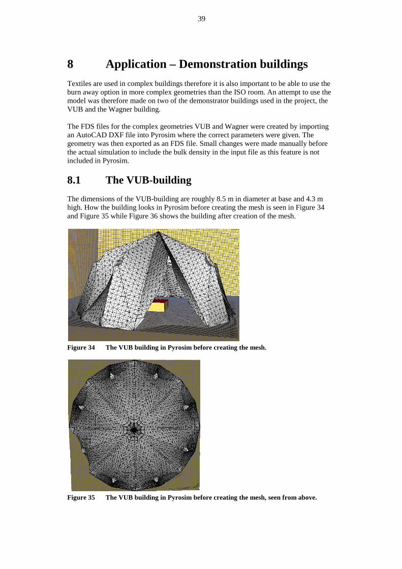
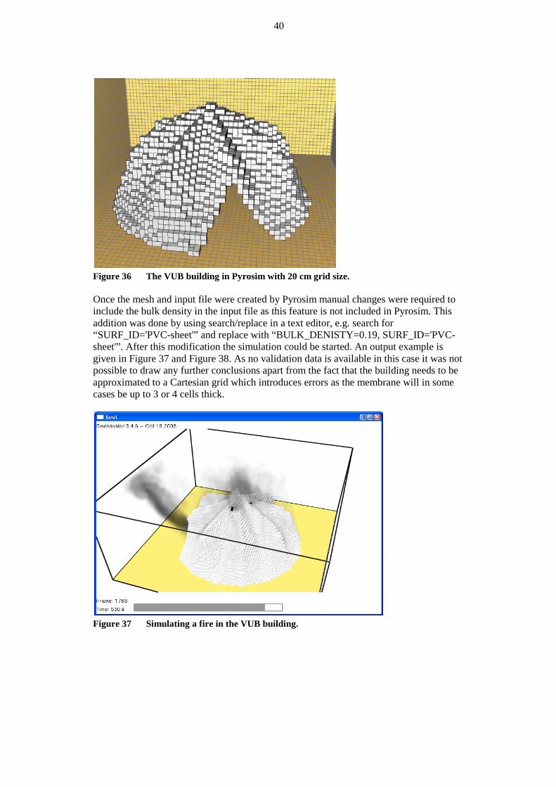
8 Application – Demonstration buildings Textiles are used in complex buildings therefore it is also important to be able to use the burn away option in more complex geometries than the ISO room. An attempt to use the model was therefore made on two of the demonstrator buildings used in the project, the VUB and the Wagner building. The FDS files for the complex geometries VUB and Wagner were created by importing an AutoCAD DXF file into Pyrosim where the correct parameters were given. The geometry was then exported as an FDS file. Small changes were made manually before the actual simulation to include the bulk density in the input file as this feature is not included in Pyrosim. 8.1 The VUB-building The dimensions of the VUB-building are roughly 8.5 m in diameter at base and 4.3 m high. How the building looks in Pyrosim before creating the mesh is seen in Figure 34 and Figure 35 while Figure 36 shows the building after creation of the mesh.
Figure 34 The VUB building in Pyrosim before creating the mesh.
Figure 35 The VUB building in Pyrosim before creating the mesh, seen from above.
40
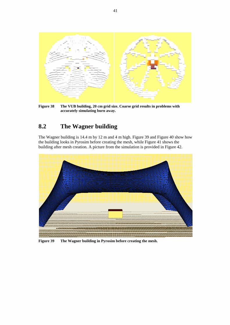
Figure 36 The VUB building in Pyrosim with 20 cm grid size. Once the mesh and input file were created by Pyrosim manual changes were required to include the bulk density in the input file as this feature is not included in Pyrosim. This addition was done by using search/replace in a text editor, e.g. search for “SURF_ID='PVC-sheet'” and replace with “BULK_DENISTY=0.19, SURF_ID='PVC-sheet'”. After this modification the simulation could be started. An output example is given in Figure 37 and Figure 38. As no validation data is available in this case it was not possible to draw any further conclusions apart from the fact that the building needs to be approximated to a Cartesian grid which introduces errors as the membrane will in some cases be up to 3 or 4 cells thick.
Figure 37 Simulating a fire in the VUB building.
41
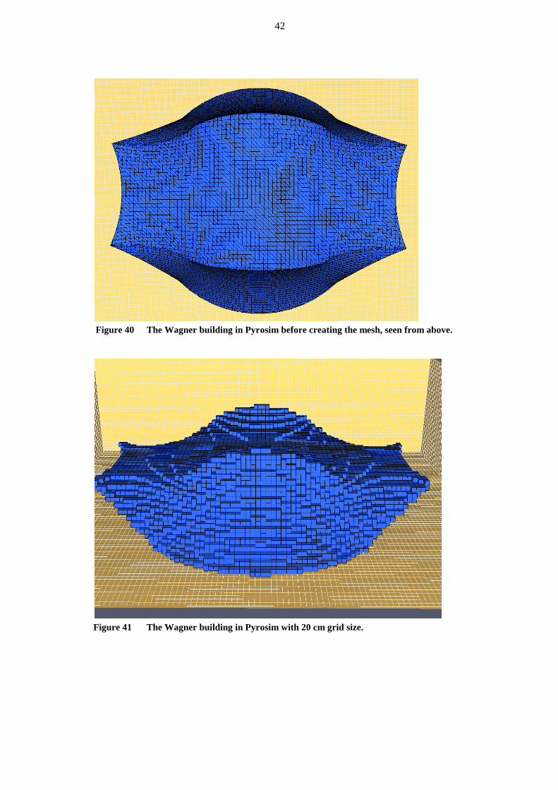
Figure 38 The VUB building, 20 cm grid size. Coarse grid results in problems with
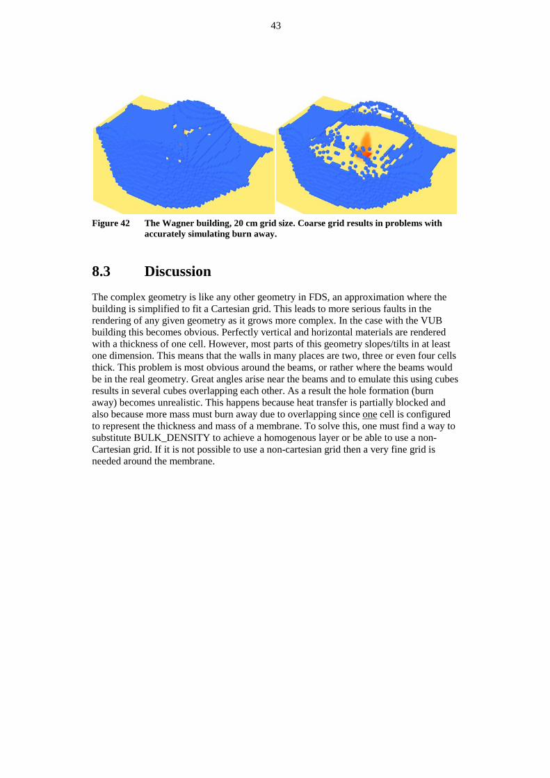
accurately simulating burn away. 8.2 The Wagner building The Wagner building is 14.4 m by 12 m and 4 m high. Figure 39 and Figure 40 show how the building looks in Pyrosim before creating the mesh, while Figure 41 shows the building after mesh creation. A picture from the simulation is provided in Figure 42.
Figure 39 The Wagner building in Pyrosim before creating the mesh.
42
Figure 40 The Wagner building in Pyrosim before creating the mesh, seen from above.
Figure 41 The Wagner building in Pyrosim with 20 cm grid size.
43
Figure 42 The Wagner building, 20 cm grid size. Coarse grid results in problems with
accurately simulating burn away. 8.3 Discussion The complex geometry is like any other geometry in FDS, an approximation where the building is simplified to fit a Cartesian grid. This leads to more serious faults in the rendering of any given geometry as it grows more complex. In the case with the VUB building this becomes obvious. Perfectly vertical and horizontal materials are rendered with a thickness of one cell. However, most parts of this geometry slopes/tilts in at least one dimension. This means that the walls in many places are two, three or even four cells thick. This problem is most obvious around the beams, or rather where the beams would be in the real geometry. Great angles arise near the beams and to emulate this using cubes results in several cubes overlapping each other. As a result the hole formation (burn away) becomes unrealistic. This happens because heat transfer is partially blocked and also because more mass must burn away due to overlapping since one cell is configured to represent the thickness and mass of a membrane. To solve this, one must find a way to substitute BULK_DENSITY to achieve a homogenous layer or be able to use a non-Cartesian grid. If it is not possible to use a non-cartesian grid then a very fine grid is needed around the membrane.
44
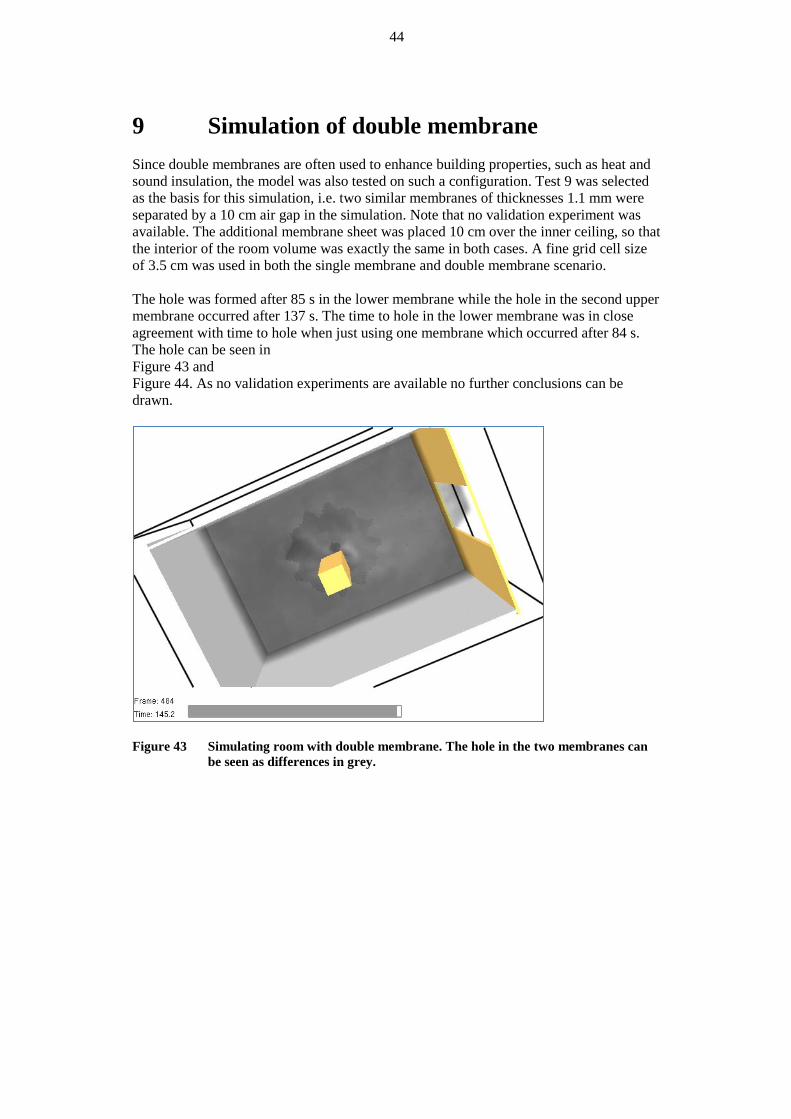
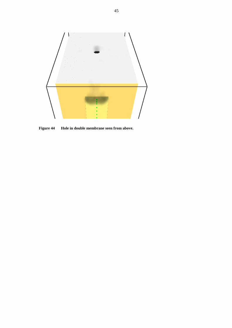
9 Simulation of double membrane Since double membranes are often used to enhance building properties, such as heat and sound insulation, the model was also tested on such a configuration. Test 9 was selected as the basis for this simulation, i.e. two similar membranes of thicknesses 1.1 mm were separated by a 10 cm air gap in the simulation. Note that no validation experiment was available. The additional membrane sheet was placed 10 cm over the inner ceiling, so that the interior of the room volume was exactly the same in both cases. A fine grid cell size of 3.5 cm was used in both the single membrane and double membrane scenario. The hole was formed after 85 s in the lower membrane while the hole in the second upper membrane occurred after 137 s. The time to hole in the lower membrane was in close agreement with time to hole when just using one membrane which occurred after 84 s. The hole can be seen in Figure 43 and Figure 44. As no validation experiments are available no further conclusions can be drawn.
Figure 43 Simulating room with double membrane. The hole in the two membranes can
be seen as differences in grey.
45
Figure 44 Hole in double membrane seen from above.
46
10 Discussion There is a great difference between test 7 and test 9 compared to test 8 and test 10. In test 7 and test 9 the flame immediately reaches the ceiling while in test 8 and test 10 the flame does not reach the ceiling until after the last HRR increase at 1200 s. This makes test 8 and test 10 more applicable to real fire scenarios, especially if fire safety is taken into account. In larger buildings of textile membranes which potentially house a high number of people, like the final applications for the type of buildings represented by the demonstrator buildings, VUB and Wagner, the initial fire process is most important. Both the experiments and simulations show that in most cases no hole will arise in the membranes used in this study until the flame reaches it. This essentially means that the evacuation conditions in the building will have reached critical levels long before smoke evacuation from a hole has begun in most situations. The feature could however become more important in more narrow scenarios like e.g. a corridor where the smoke venting might have a larger influence on the evacuation situation. In addition there might be other material that opens up at a lower temperature than those used in this study which might be able to benefit from the opening up of a hole in other evacuation situations. The main sources of error can be divided into two parts, i.e.: those pertaining to the validation experiments and those pertaining to the simulations. Concerning experimental errors one important drawback is that only one experiment of each configuration was conducted, which means there is an unknown uncertainty in temperature readings and probably a substantial uncertainty in time to hole opening and size of hole. In terms of the errors in simulations, the burn away option is a coarse simplification of a very complicated combustion process. In this case, we try to use this simple model to open up a hole which can arise from a number of different reasons or combination thereof, such as pyrolysation or burning off, but also melting and shrinking of the material or due to local weaknesses in the material. The burn away option does not account for in particular the latter three. During the validation experiments pieces of the membrane was seen too fall down and molten membrane was seen to drip from the roof. This indicates that the holes growth is not only dependent on the burning away of the membrane but also physical melting and/or break-down. The simulation with the burn away option relies on very good input parameters. There is a considerable margin of error in choosing the pyrolysis range from a TGA result as well as in extracting input from the results of the Cone Calorimeter. Statistical foundation is not sufficient when only one or a pair of tests is conducted. Despite the limited number of experiments the required parameters varied considerably in some cases which highlights the uncertainties in the input data even more. The combined margin of error in each of the input parameters results in an even greater margin of error in the output. The simulated materials are built up of two kinds of polyester threads, one lengthways and one edgeways, coated in polyvinyl chloride, PVC. These two threads probably have different strength, sustainability and melting point. When heated, the membrane will at first give off plasticizers. Then the PVC will break down and chlorine will leave in the form of hydrogen chloride. This makes the material weaker and indicates that linear strain is important for the hole formation, a process which occurs before actual ignition effects the evolution of holes. Finally, the simulations also showed that the results are sensitive to the random number generator, RND12. This can confuse the user when investigating the influence of different
47
parameters. Note, however that the RND sensitivity was not observed for the short time to hole but only for test 8 and test 10. 10.1 Further studies The model is highly dependent on obtaining/estimating correct input data. The uncertainty in the input data used in this study was large and there is room for improvement. A number of different suggestions for future work to improve the application of the model are given below:
• The determination of, e.g. ΔHc from the Cone Calorimeter could be improved. One could perhaps place several layers above each other and thereby decrease the uncertainty. The use of a lower incident radiation could also be further explored.
• A greater number of repetitions of the experiments, both small scale for input
data and full scale validation experiments, is required in order to validate the model further.
• The grid dependence of the simulations needs to be investigated further as no grid independent solution was found in this study.
• Further work is needed on the use of Pyrolysis Model II as this has not been studied to the same extent as Pyrolysis Model I, e.g. further studies are needed to straighten out how residue works in Pyrolysis Model II.
• More detailed investigation of the application of CFD simulations to complex geometries is needed. Indeed, to acquire satisfying results from simulations with the complex geometries a finer grid size is needed than that used here. Such a simulation will require a fast CPU and a substantial amount of random-access memory (RAM) to run efficiently. It would be wise to consider dividing such a room in several meshes and use parallel computing to save calculation time. The use of multiple meshes and parallel computing does however need validation.
• Experimental data concerning the fire development and performance of textile membranes in complex geometries is needed both to understand the impact of complex geometries on the function of a textile membrane and for comparison to simulations.
• It would be useful if FDS could handle several fuels.
• Both test and simulations were conducted at around 20°C ambient temperature,
no investigations have been made on how the material and model works in other temperatures like winter conditions. This could be interesting for further studies also how aging of the material influences the performance.
48
11 Conclusions Results show that it is possible to use the burn away option in FDS to model the opening up of a hole in textile membranes, including the case where double membranes are used. The quality of the results compared to the validation experiments has varied for the pyrolysis models used and the different test conditions simulated. No simulation has perfectly predicted the validation experiments and in some cases the difference has been significant. Pyrolysis Model II with the Arrhenius type of reaction rate seems to have a greater potential to simulate the experimental results than Pyrolysis Model I with the prescribed burn rate. Further, it has not been possible to find grid independent solutions. Great precaution should be taken when using the burn away option for fire safety design purposes. There are uncertainties in finding the correct input data, especially determining the heat of combustion from the Cone Calorimeter tests and the width of the pyrolysis range from the Thermogravimetric Analysis. When using a wide possible range of several parameters, where most are sensitive to change, it becomes more difficult to find the true input and successfully simulate the validation experiments. Verification from validation experiments is always needed in any application of the model for calculation of membrane hole-opening in a fire safety engineering application. It is possible to import complex geometries to FDS by using auxiliary programs such as Pyrosim and use the burn away option as well. However, the fact that only Cartesian coordinates are allowed in FDS is a significant problem as complex geometries with sloped and curved surfaces are unsuited to a Cartesian description. At the moment this makes it impossible to accurately simulate complex geometries for fire safety design purposes. There is a need for finer grids when working with complex geometries. However, the CPU time was 10 days for the geometries used on one of today’s fastest personal computers. The cluster could not simulate this geometry at all using the serial version of FDS because of lack of memory. It would have been possible to simulate with the parallel version but this was not tried as it would require more studies concerning the interface between the different grids. The feature of a hole opening in a textile membrane due to burning away was considered important for fire safety design of buildings with these membranes. From the results of this study the conclusion can be drawn that an opening for such a purpose will not occur until the flame reaches the ceiling for the materials used in this study. This means that when the hole reaches a size that will evacuate a considerable amount of smoke the conditions in the room are not acceptable for evacuation. This conclusion is valid for the materials tested in this study and for applications like assembly halls etc. The hole-opening feature could have effect on more narrow evacuation situations like a corridor. In addition there might be materials that open up earlier in a fire which could potentially influence also other evacuation situations. The triggering of a smoke vent for evacuation purposes always include opening up also for supply air in order to avoid an under pressure in the room. This feature is, however, not accomplished through the natural hole opening of the membranes.
49
References 1. McGrattan K., et.al, “Fire Dynamics Simulator (Version 5) User’s Guide”,
NIST Special Publication 1019-5, 2010.
2. http://www.thunderheadeng.com/pyrosim, 5/28/2010.
3. Forney G.P., “Smokeview (Version 5) – A Tool for Visualizing Fire Dynamics Simulation Data Volume I:User’s Guide”, NIST Special Publication 1017-1, 2010.
4. ISO 13784-1:2002, Reaction-to-fire tests for sandwich panel building systems -- Part 1: Test method for small rooms.
5. ISO 9705:1993, Fire tests -- Full-scale room test for surface products.
6. Andersson and Blomqvist, “Large-scale fire tests with textile membranes for building applications, SP Technical Note 2010:03, Borås 2010.
7. Wickström, U. “ Measurement of incident radiant heat flux with the plate thermometer”, 12 international Fire Science & Engineering Conference INTERFLAM 2010, Nottingham 2010, pp 327-340, Interscience London 2010.
8. ISO 5660-1:2002, Reaction-to-fire tests - Heat release, smoke production and mass loss rate - Part 1: Heat release rate (cone calorimeter method).
9. ISO22007-2, Plastics- Determination of thermal conductivity and thermal diffusivity, Part2: Transient plane heat source (hot disc) method.
10. http://www.engineeringtoolbox.com
11. McGrattan K., Floyd J., Forney G., Baum H., and Hostikka, S., “Improved Radiation and Combustion Routines for a Large Eddy Simualtion Fire Model”, Fire Safety Science – Proceedings of the Seventh International Symposium, International Association for Fire Safety Science, Boston MA, 2003.
12. McGrattan, K., Building and Fire Research Laboratory, NIST.
50
Appendix A - Fire Safety Engineering in contex-T Prescriptive fire safety regulations which in detail regulate the design and classification of building components will, for some applications, exclude the use of textile materials which do not conform to the required fire rating. A performance based approach to comply with the overall fire safety level of the building can be a valid alternative for such applications. Fire safety regulations are basically prescriptive in many countries. However, a performance based approach is allowed in several European countries. Answers to a questionnaire which was sent to the contex-T partners indicated that performance based FSE is allowed for textile buildings in Sweden, Italy and Germany. However, the answer frequency on the questionnaire was not 100% and knowledge of national fire regulations by the different partners could not be expected to be exhaustive. A better source of information on the general applicability of performance based FSE is a report by FORUM. Here it was reportedii that the European countries that can be classified as performance based are: the United Kingdom, Sweden, and Norway. Other countries allowing FSE alternatives include: Belgium, France, Italy, Luxembourg, Netherlands, Germany, Denmark, Ireland, Greece, Portugal, Spain, Austria, Finland, and Switzerland. Performance based FSE can therefore be a valid approach in many European countries. Generally, performance based regulations allow the building contractor to choose an appropriate design method to accomplish fire protection in accordance with the safety level defined in the regulations. For most buildings there are two alternative methods that can be used in performance based fire safety work:
• prescriptive design or • analytical design.
Prescriptive design is, in principle, the same method as was used prior to the introduction of performance based requirements. Prescriptive design assumes that all the requirements and general recommendations for the object in question are set out to be fully met. When using prescriptive design it is not possible to make any technical exchanges in addition to those already given in the published regulations. If any other technical exchanges are made the design is considered to be an analytical one. One reason to abandon prescriptive design is that a more cost effective design might be possible through a technical exchange. An even more common reason to use analytical design is that fire safety according to prescriptive standards places limitations on the design regarding, for example, architectural objectives or activity. This is the most important factor determining the need to apply analytical design to textile buildings. A comprehensive requirement when using analytic design is that the fire safety accomplished in a building should be as good as or better than if all the prescriptive requirements were set out to be met. A disadvantage when using analytic design is that this method requires more time and knowledge of the designer than prescriptive design. When using prescriptive design the requirements to verify the results are low. This design method is simple, well known and is in most cases results in a conservative fire safety solution. ii NIST Special Publication 1061, ” Forum Workshop on Establishing the Scientific Foundation for Performance-Based Fire Codes: Proceedings”, December 2006.
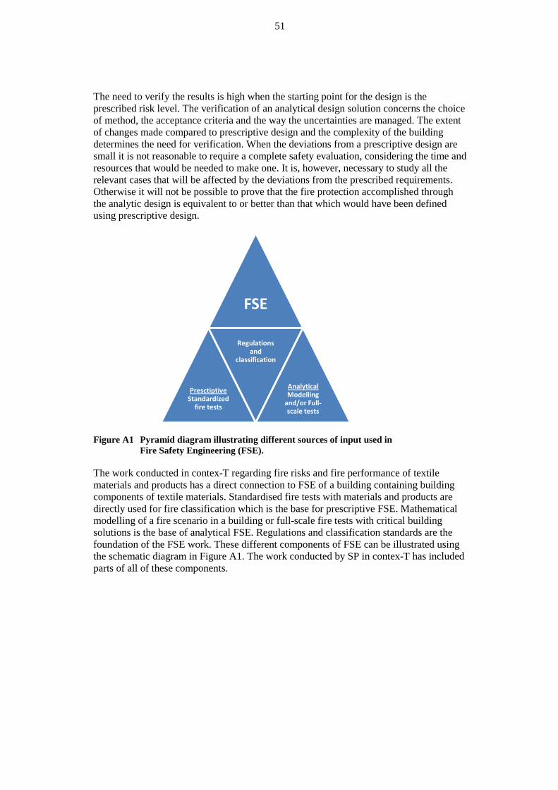
51
The need to verify the results is high when the starting point for the design is the prescribed risk level. The verification of an analytical design solution concerns the choice of method, the acceptance criteria and the way the uncertainties are managed. The extent of changes made compared to prescriptive design and the complexity of the building determines the need for verification. When the deviations from a prescriptive design are small it is not reasonable to require a complete safety evaluation, considering the time and resources that would be needed to make one. It is, however, necessary to study all the relevant cases that will be affected by the deviations from the prescribed requirements. Otherwise it will not be possible to prove that the fire protection accomplished through the analytic design is equivalent to or better than that which would have been defined using prescriptive design.
Figure A1 Pyramid diagram illustrating different sources of input used in Fire Safety Engineering (FSE).
The work conducted in contex-T regarding fire risks and fire performance of textile materials and products has a direct connection to FSE of a building containing building components of textile materials. Standardised fire tests with materials and products are directly used for fire classification which is the base for prescriptive FSE. Mathematical modelling of a fire scenario in a building or full-scale fire tests with critical building solutions is the base of analytical FSE. Regulations and classification standards are the foundation of the FSE work. These different components of FSE can be illustrated using the schematic diagram in Figure A1. The work conducted by SP in contex-T has included parts of all of these components.
FSE
PresctiptiveStandardized
fire tests
Regulations and
classification
AnalyticalModelling
and/or Full-scale tests

SP Technical Research Institute of Sweden Box 857, SE-501 15 BORÅS, SWEDEN Telephone: +46 10 516 50 00, Telefax: +46 33 13 55 02 E-mail: [email protected], Internet: www.sp.se www.sp.se
Fire Technology SP Report 2010:54 ISBN 978-91-86319-94-6 ISSN 0284-5172
More information about publications published by SP: www.sp.se/publ
SP Technical Research Institute of Sweden Our work is concentrated on innovation and the development of value-adding technology. Using Sweden's most extensive and advanced resources for technical evaluation, measurement technology, research and development, we make an important contribution to the competitiveness and sustainable development of industry. Research is carried out in close conjunction with universities and institutes of technology, to the benefit of a customer base of about 9000 organisations, ranging from start-up companies developing new technologies or new ideas to international groups.