A Business Model for Retail Aggregation of Responsive Load to Produce Wholesale Products

CERTS Project Review Cornell University, August 5-6, 2014

Project Lead: Shmuel S. Oren - Industrial Engineering & Operations Research (IEOR) UC Berkeley Team Members: Clay Campaign – Graduate student, IEOR Kostas Margellos– Post Doctoral Fellow, IEOR

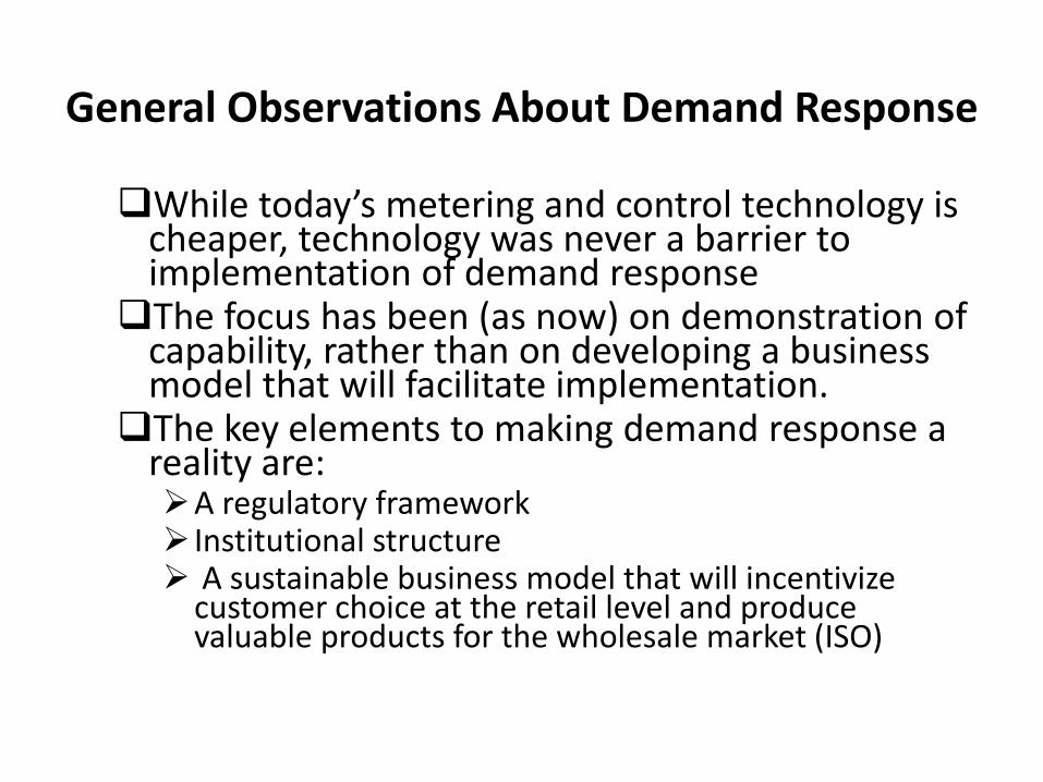
General Observations About Demand Response

While today’s metering and control technology is cheaper, technology was never a barrier to implementation of demand response The focus has been (as now) on demonstration of

capability, rather than on developing a business model that will facilitate implementation. The key elements to making demand response a

reality are: A regulatory framework Institutional structure A sustainable business model that will incentivize

customer choice at the retail level and produce valuable products for the wholesale market (ISO)

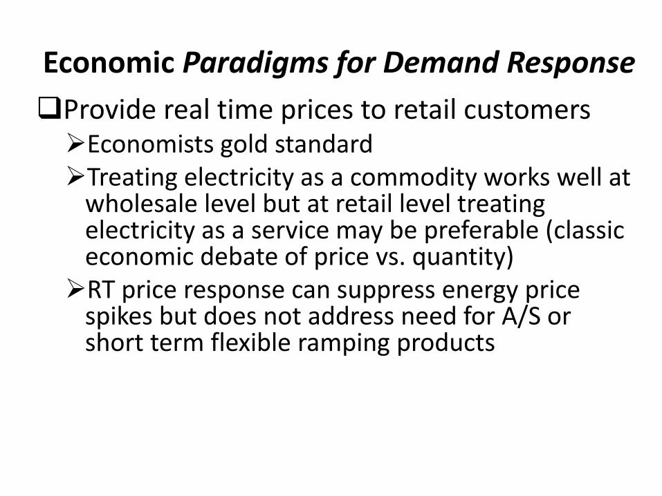
Economic Paradigms for Demand Response Provide real time prices to retail customers Economists gold standard Treating electricity as a commodity works well at

wholesale level but at retail level treating electricity as a service may be preferable (classic economic debate of price vs. quantity) RT price response can suppress energy price

spikes but does not address need for A/S or short term flexible ramping products

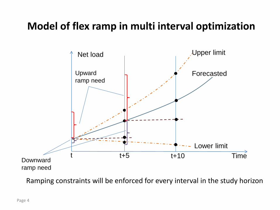
Model of flex ramp in multi interval optimization

Ramping constraints will be enforced for every interval in the study horizon

Page 4

Forecasted

Upper limit

Lower limit t+5 t Time

Net load

Upward ramp need

Downward ramp need

t+10

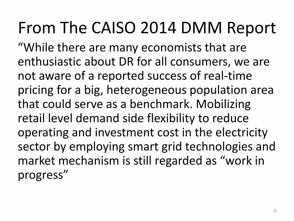
From The CAISO 2014 DMM Report “While there are many economists that are enthusiastic about DR for all consumers, we are not aware of a reported success of real-time pricing for a big, heterogeneous population area that could serve as a benchmark. Mobilizing retail level demand side flexibility to reduce operating and investment cost in the electricity sector by employing smart grid technologies and market mechanism is still regarded as “work in progress”

5

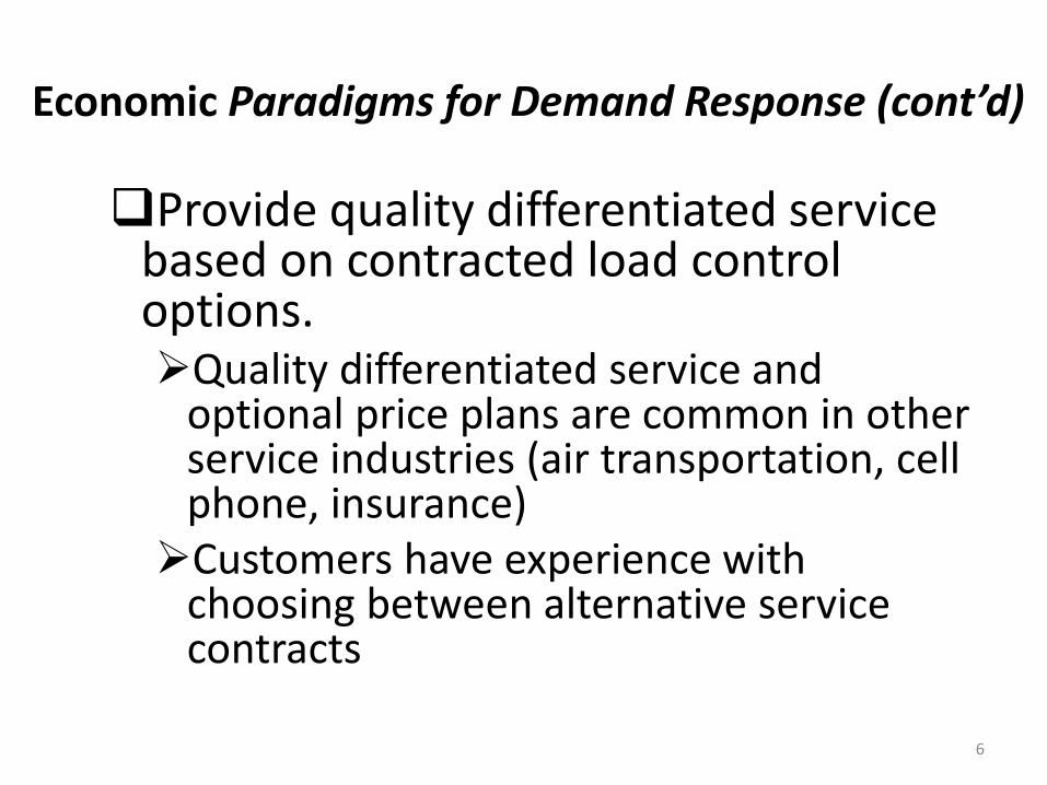
Economic Paradigms for Demand Response (cont’d)

Provide quality differentiated service based on contracted load control options. Quality differentiated service and

optional price plans are common in other service industries (air transportation, cell phone, insurance) Customers have experience with

choosing between alternative service contracts

6

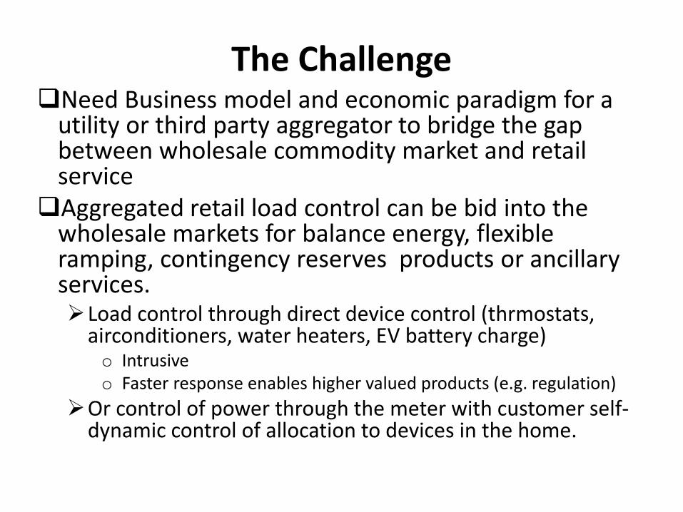
The Challenge Need Business model and economic paradigm for a

utility or third party aggregator to bridge the gap between wholesale commodity market and retail service Aggregated retail load control can be bid into the

wholesale markets for balance energy, flexible ramping, contingency reserves products or ancillary services. Load control through direct device control (thrmostats,

airconditioners, water heaters, EV battery charge) o Intrusive o Faster response enables higher valued products (e.g. regulation)

Or control of power through the meter with customer self-dynamic control of allocation to devices in the home.

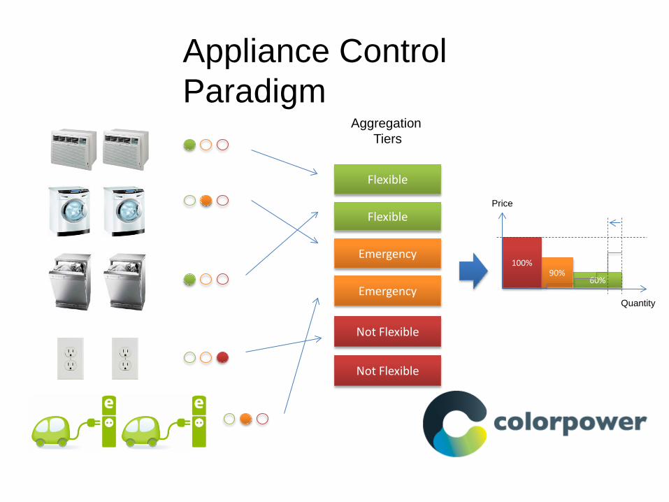
Flexible

Flexible

Emergency

Emergency

Not Flexible

Not Flexible

Aggregation Tiers

60% 90%

100%

Price

Quantity

Appliance Control Paradigm

Aggregator

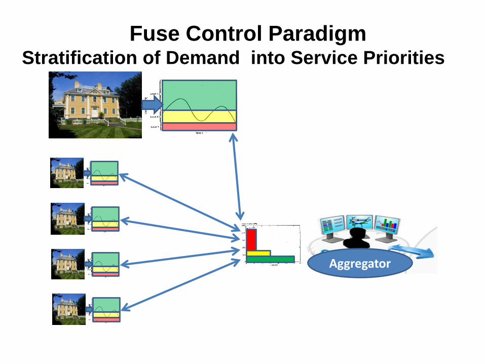
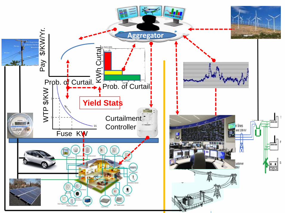
Fuse Control Paradigm Stratification of Demand into Service Priorities

Fuse KW

WTP

$/K

W Aggregator

Prob. of Curtail.

Pay

$/K

W/Y

r.

Prob. of Curtail. K

Wh

Cur

tal.

Curtailment Controller

Yield Stats

Necessary Conditions

• Renewable resources must have incentives to firm up their supply. – Eliminate feed-in tariffs and require

renewables to schedule (at least in the 15 minute market)

– Enable firmed up renewable resources (bundled with flexible load) to receive capacity payments

• Implement demand charges at retail level which can be adjusted based on curtailment options

11

Research Activities

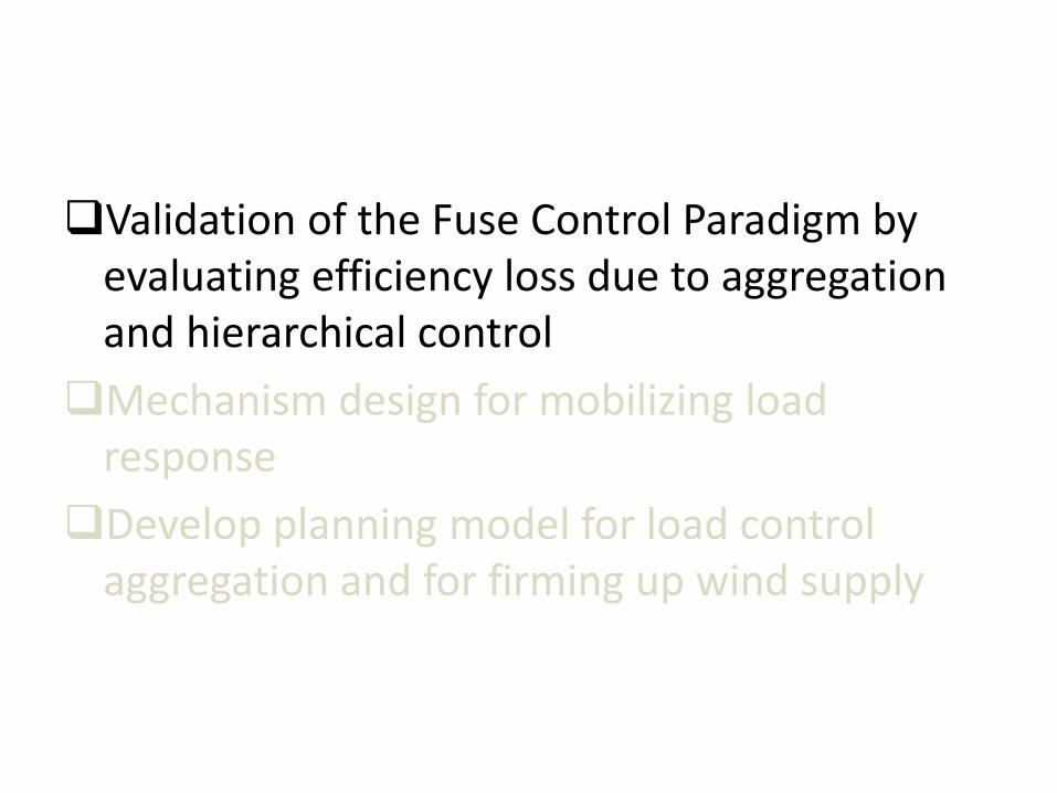
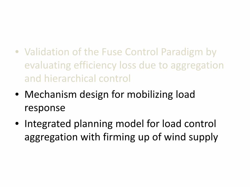
Validation of the Fuse Control Paradigm by evaluating efficiency loss due to aggregation and hierarchical control Mechanism design for mobilizing load

response Integrated planning model for load control

aggregation with firming up of wind supply

Validation of the Fuse Control Paradigm by evaluating efficiency loss due to aggregation and hierarchical control Mechanism design for mobilizing load

response Develop planning model for load control

aggregation and for firming up wind supply

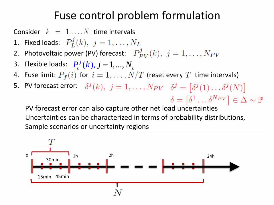
Fuse control problem formulation Consider time intervals 1. Fixed loads: 2. Photovoltaic power (PV) forecast: 3. Flexible loads: 4. Fuse limit: for (reset every time intervals) 5. PV forecast error:

PV forecast error can also capture other net load uncertainties Uncertainties can be characterized in terms of probability distributions, Sample scenarios or uncertainty regions

( ), 1,..., cj

cP jk N=

0 1h 2h 24h

15min

30min

45min

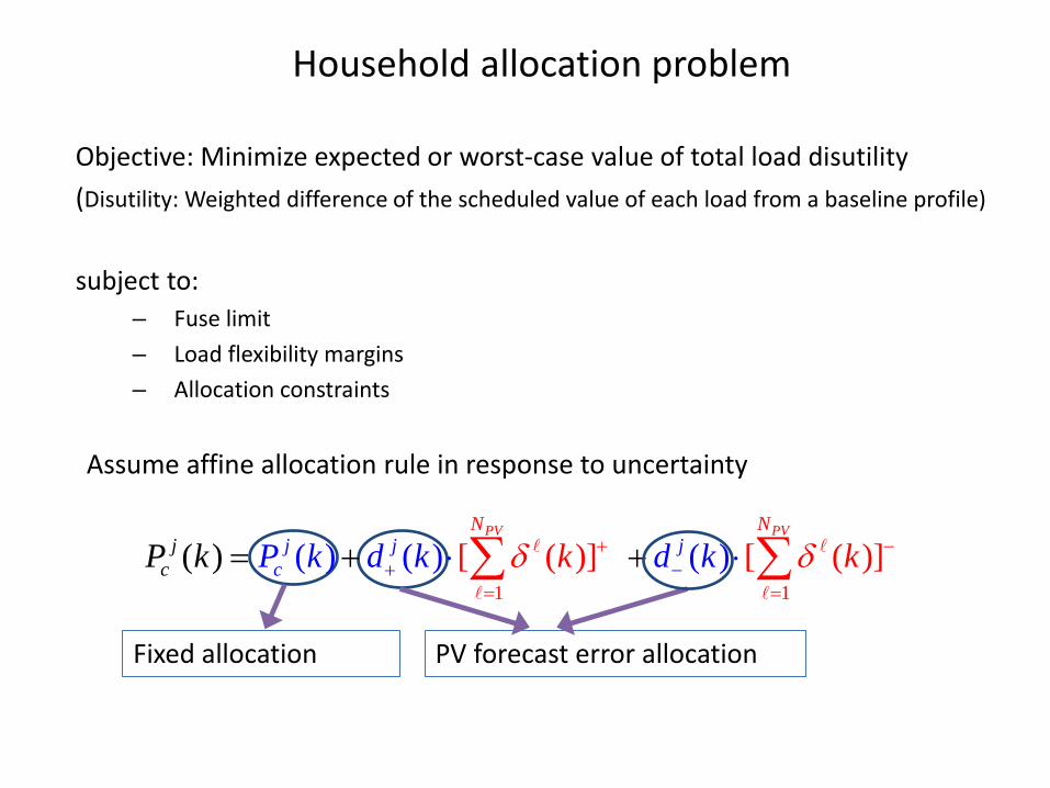
Fixed allocation PV forecast error allocation

1 1[ ( )] ( ) ( ) ( )( [) ( )]

PV PVj j j

N

c

N

cjP k d k d kkP k kδ δ+ −

=+

=−= + +⋅ ⋅∑ ∑

Objective: Minimize expected or worst-case value of total load disutility (Disutility: Weighted difference of the scheduled value of each load from a baseline profile)

subject to:

– Fuse limit – Load flexibility margins – Allocation constraints

Assume affine allocation rule in response to uncertainty

Household allocation problem

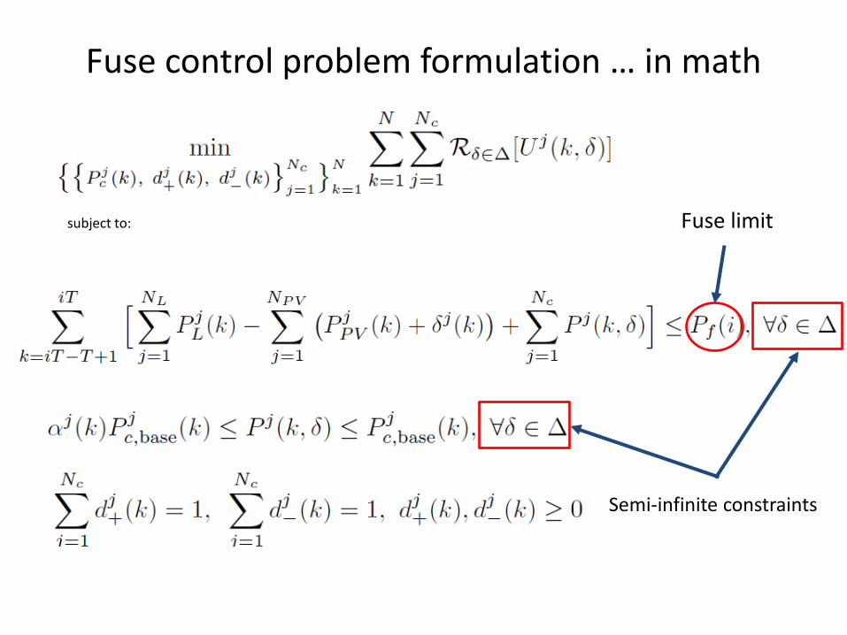
Fuse control problem formulation … in math

subject to: Fuse limit

Semi-infinite constraints

Fuse control problem formulation

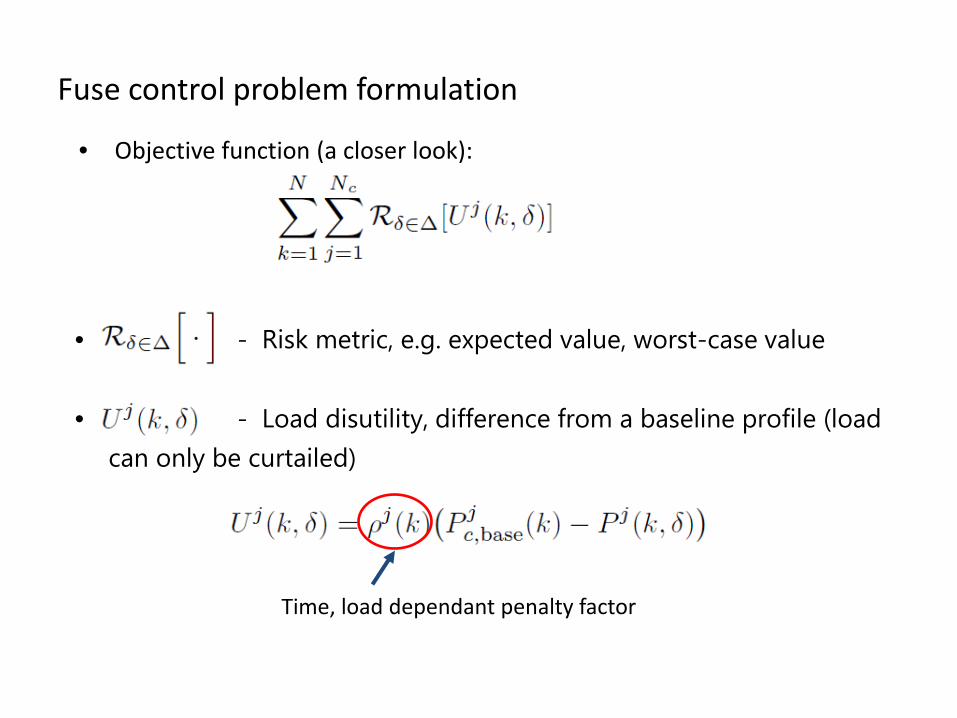
• Objective function (a closer look):

• - Risk metric, e.g. expected value, worst-case value

• - Load disutility, difference from a baseline profile (load can only be curtailed)

Time, load dependant penalty factor

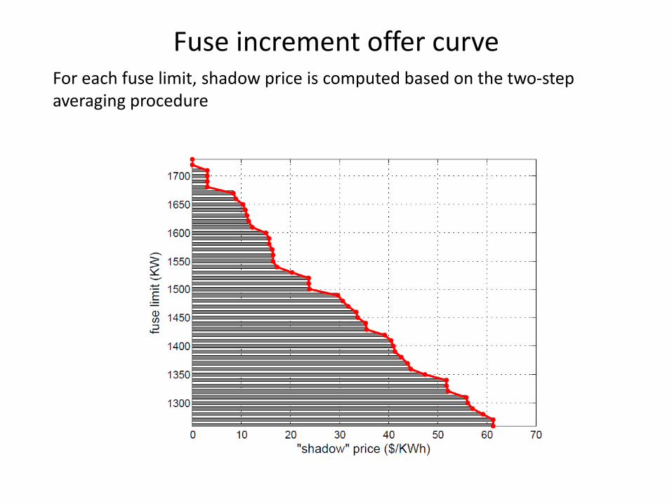
Fuse increment offer curve For each fuse limit, shadow price is computed based on the two-step averaging procedure

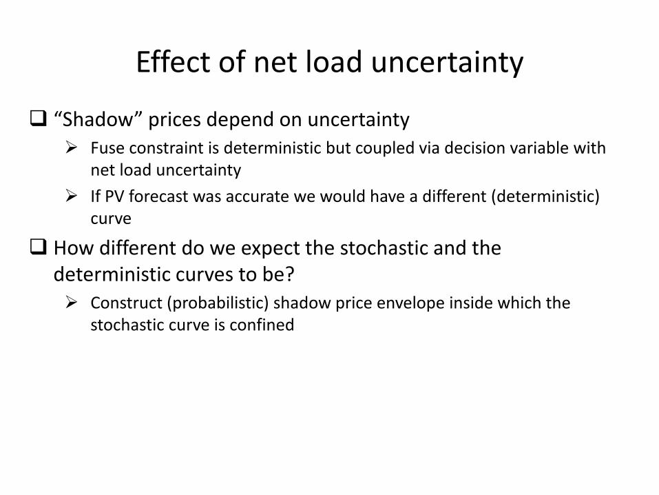
Effect of net load uncertainty

“Shadow” prices depend on uncertainty Fuse constraint is deterministic but coupled via decision variable with

net load uncertainty If PV forecast was accurate we would have a different (deterministic)

curve

How different do we expect the stochastic and the deterministic curves to be? Construct (probabilistic) shadow price envelope inside which the

stochastic curve is confined

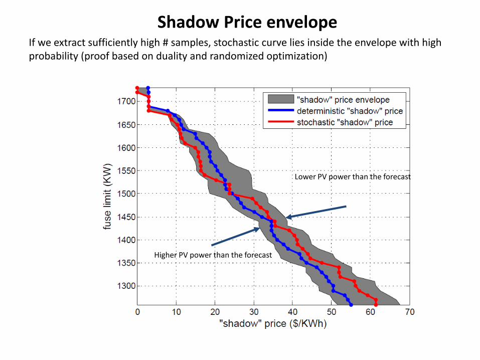
Shadow Price envelope If we extract sufficiently high # samples, stochastic curve lies inside the envelope with high probability (proof based on duality and randomized optimization)

Lower PV power than the forecast

Higher PV power than the forecast

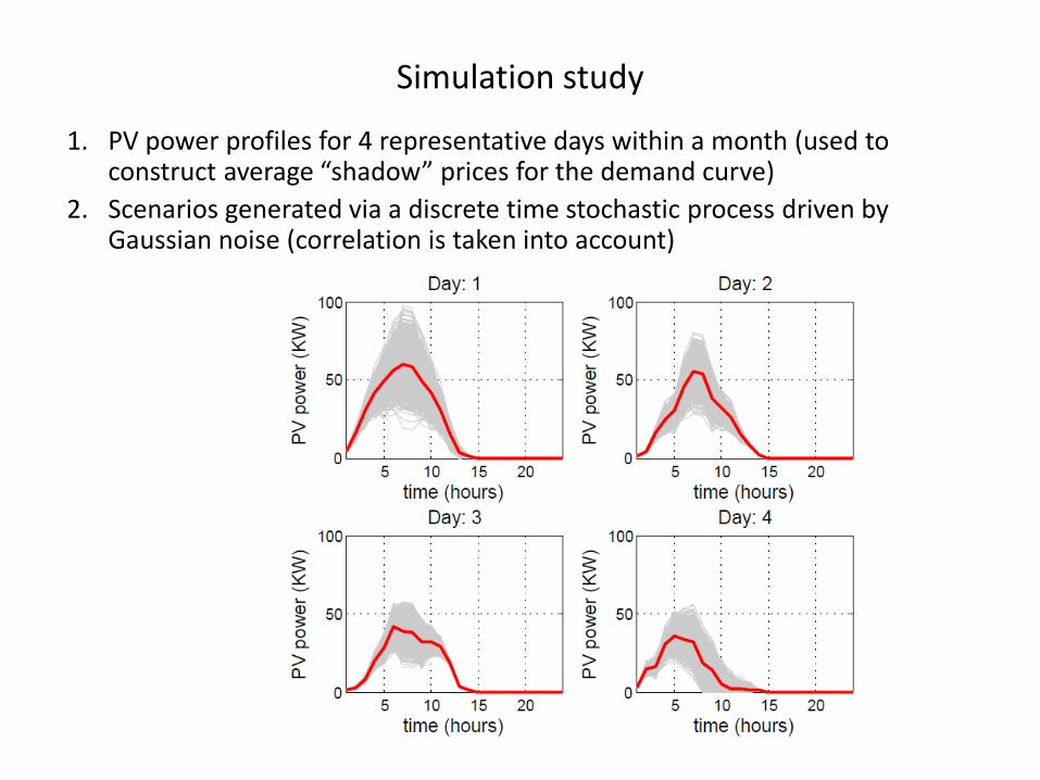
Simulation study

1. PV power profiles for 4 representative days within a month (used to construct average “shadow” prices for the demand curve)

2. Scenarios generated via a discrete time stochastic process driven by Gaussian noise (correlation is taken into account)

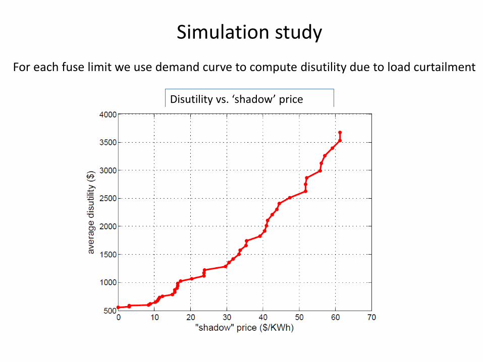
Simulation study For each fuse limit we use demand curve to compute disutility due to load curtailment

Disutility vs. ‘shadow’ price

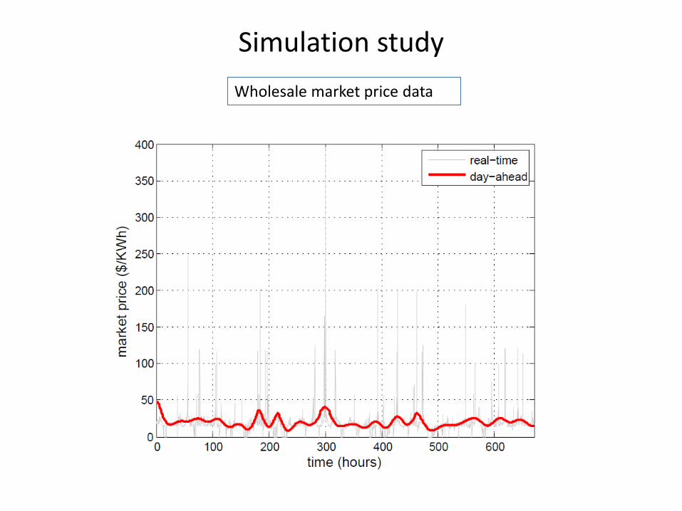
Simulation study Wholesale market price data

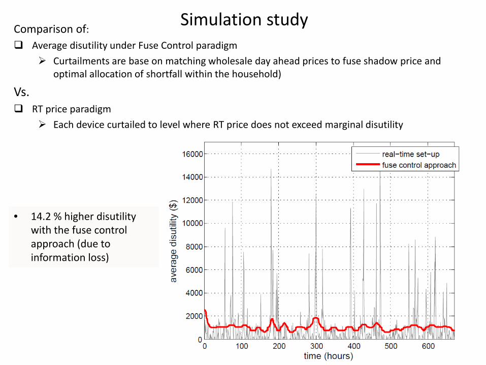
Simulation study Comparison of: Average disutility under Fuse Control paradigm

Curtailments are base on matching wholesale day ahead prices to fuse shadow price and optimal allocation of shortfall within the household)

Vs. RT price paradigm

Each device curtailed to level where RT price does not exceed marginal disutility

• 14.2 % higher disutility with the fuse control approach (due to information loss)

• Validation of the Fuse Control Paradigm by evaluating efficiency loss due to aggregation and hierarchical control

• Mechanism design for mobilizing load response

• Integrated planning model for load control aggregation with firming up of wind supply

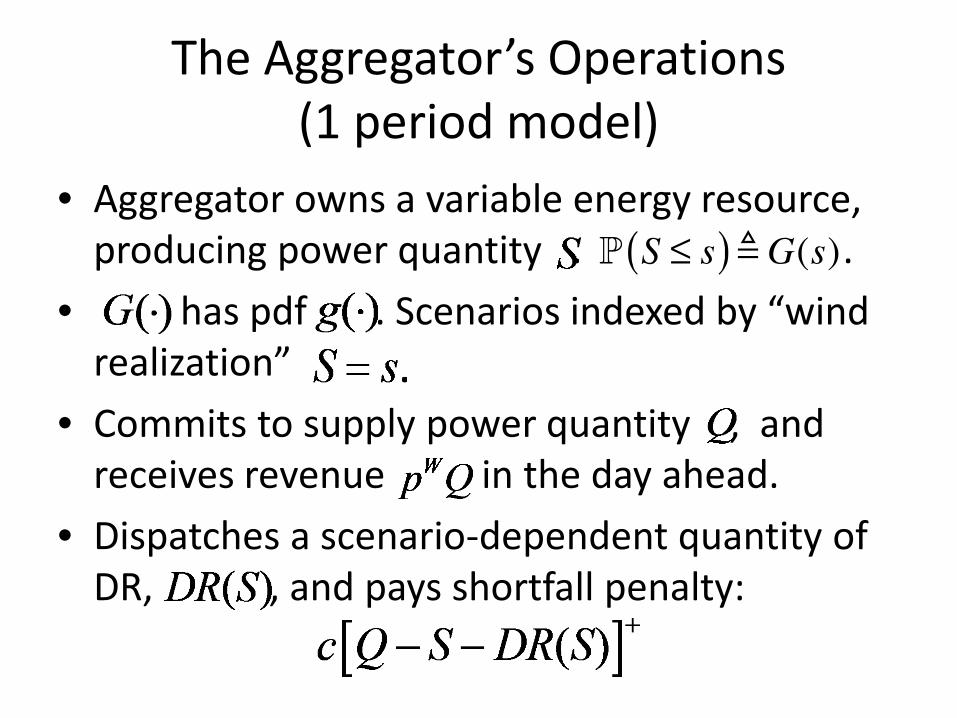
The Aggregator’s Operations (1 period model)

• Aggregator owns a variable energy resource, producing power quantity . .

• has pdf . Scenarios indexed by “wind realization”

• Commits to supply power quantity , and receives revenue in the day ahead.

• Dispatches a scenario-dependent quantity of DR, , and pays shortfall penalty:

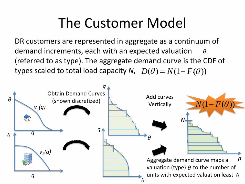
The Customer Model DR customers are represented in aggregate as a continuum of demand increments, each with an expected valuation (referred to as type). The aggregate demand curve is the CDF of types scaled to total load capacity N, . ( ) (1 ( ))D N Fθ θ= −

Aggregate demand curve maps a valuation (type) to the number of units with expected valuation least

q

q

q

Obtain Demand Curves (shown discretized)

Add curves Vertically

N

(1 ( ))N F θ−v1(q)

v2(q)

q

𝜃𝜃

𝜃𝜃 𝜃𝜃

𝜃𝜃

𝜃𝜃

𝜃𝜃

𝜃𝜃 𝜃𝜃

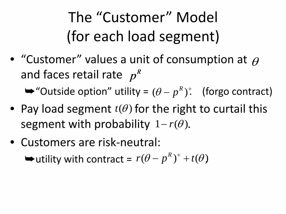
The “Customer” Model (for each load segment)

• “Customer” values a unit of consumption at and faces retail rate ➥“Outside option” utility = . (forgo contract)

• Pay load segment for the right to curtail this segment with probability .

• Customers are risk-neutral: ➥utility with contract = .

θ

( )t θ1 ( )r θ−

) (( )Rr p tθ θ+ +−

( )Rpθ +−

0 10 20 30 40

Demand Resource Supply Resource

Demand Side

Committed Power

Demand Segments or Tranches

𝑥𝑥 MW

Demand Aggregation

Supply Pooling

Demand & Supply Coordination

Renewables Ex-post energy composition of offer RT Market / Penalty

The Wholesale Product Offered by the Aggregator

Wholesale Electricity Markets

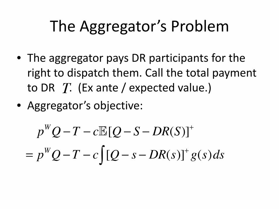
The Aggregator’s Problem

• The aggregator pays DR participants for the right to dispatch them. Call the total payment to DR . (Ex ante / expected value.)

• Aggregator’s objective:

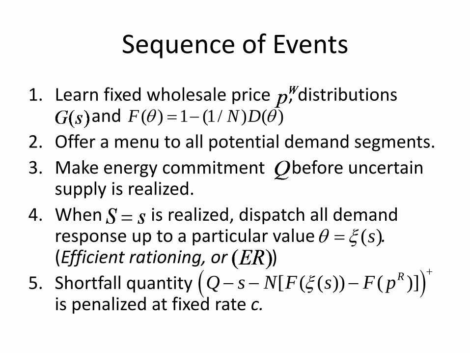
Sequence of Events

1. Learn fixed wholesale price , distributions d and

2. Offer a menu to all potential demand segments. 3. Make energy commitment before uncertain

supply is realized. 4. When S = s is realized, dispatch all demand

response up to a particular value . (Efficient rationing, or )

5. Shortfall quantity is penalized at fixed rate c.

( ) 1 (1/ ) ( )F N Dθ θ= −

( )( )) ([ ( )]RsQ s N F pF ξ+

−− −

( )sθ ξ=

Mechanism Design Setup Invoking the “Revelation Principle’ we can represent the contract-menu as a function of type. We pay a load segment to reduce its service reliability from 1 to . (Due to monotonicity this implies a unique menu of contract options presented as ) A menu must satisfy: (WLOG by the Revelation Principle): Proposition 1. Necessary condition for (IC

1.

2.

3.

4.

( ) ( ) ()( )R Rt r p pθθ θ θ + +≥ −+ −

( )t θ( )r θ

( ) ( )( ˆ ˆ( ) ( )() )R Rt r p t r v pθ θ θ θ θ+ ++ − + −≥ [0, ].θ θ∀ ∈ˆ, .θ θ∀

( ) non-decreasing over [ , ]Rr p θ⋅

( ) non-increasing over [ , ]Rt p θ⋅

( ) (0) [ ( ) ( )]Rp

t t r r z dzθ

θθ θ

∧= − −∫

( ) (0) ( )Rp

u u r z dzθ

θθ

∧= + ∫

( )t r

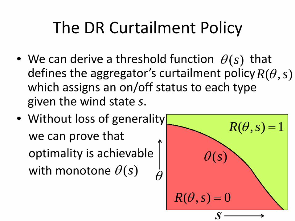
The DR Curtailment Policy

• We can derive a threshold function that defines the aggregator’s curtailment policy which assigns an on/off status to each type given the wind state s.

• Without loss of generality we can prove that optimality is achievable with monotone

( , ) 1R sθ =

( , ) 0R sθ =

θ

( , )R sθ( )sθ

( )sθ( )sθ

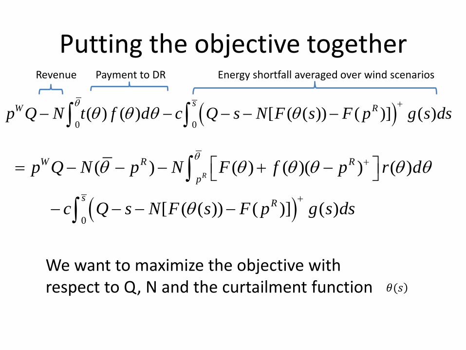
Putting the objective together

( )0 0

( ) ( ( )) ( )( )]) [ (sW Rp Q N t f d c Q s s F pN F g s ds

θθ θ θθ

+− − −− −∫ ∫

( )0

( ) ) ( )

( )

( ) ( )(

[ ( ) ( )] ( )

R

W R R

p

s R

p Q F f p r

c Q s N F

N

g

p N d

s s dsF p

θθ θ θ

θ

θ θ θ +

+

= − + −

− − −

− −

−

∫

∫

Energy shortfall averaged over wind scenarios Payment to DR Revenue

We want to maximize the objective with respect to Q, N and the curtailment function 𝜃𝜃(𝑠𝑠)

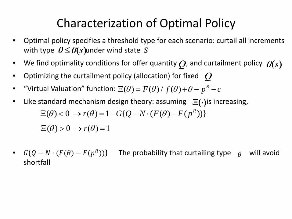
Characterization of Optimal Policy • Optimal policy specifies a threshold type for each scenario: curtail all increments

with type under wind state

• We find optimality conditions for offer quantity , and curtailment policy .

• Optimizing the curtailment policy (allocation) for fixed

• “Virtual Valuation” function:

• Like standard mechanism design theory: assuming is increasing,

• The probability that curtailing type will avoid shortfall

( ) ( ) / ( ) RF f p cθ θ θ θΞ = + − −

( ) 0 ( ) 1 { ( ( ) ( ))}Rr G Q N F F pθ θ θΞ < → = − − ⋅ −

( ) 0 ( ) 1rθ θΞ > → =

s

𝐺𝐺{𝑄𝑄 − 𝑁𝑁 ⋅ (𝐹𝐹(𝜃𝜃) − 𝐹𝐹(𝑝𝑝𝑅𝑅))} 𝜃𝜃

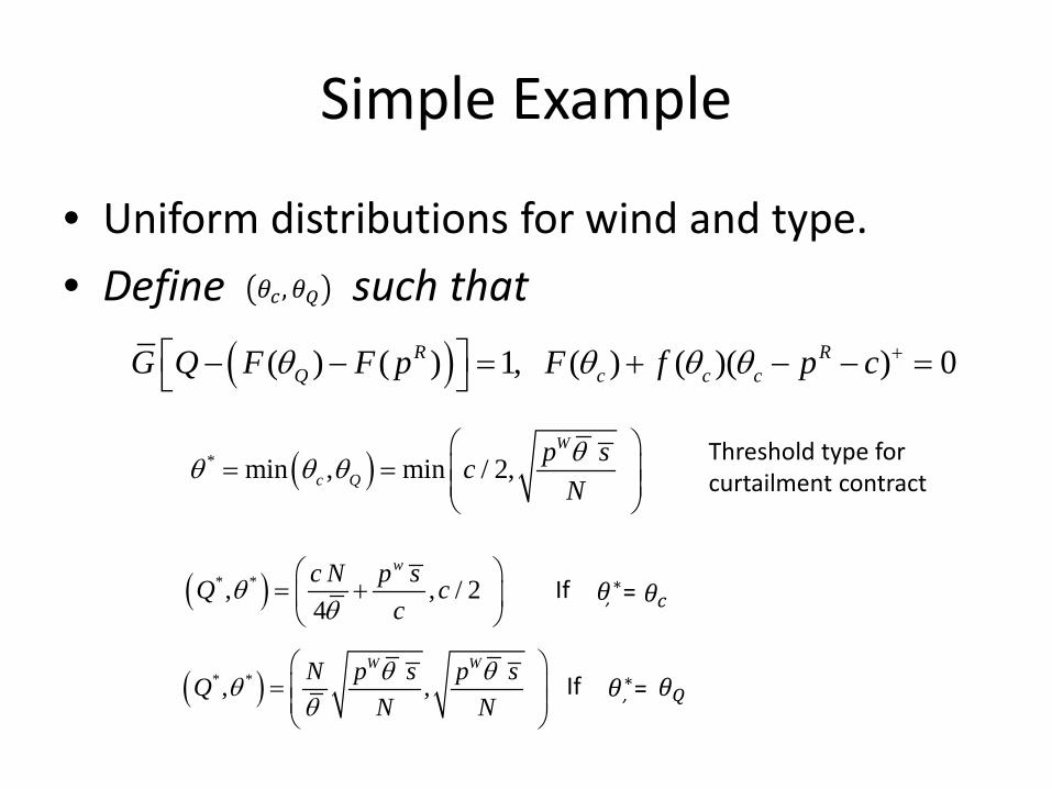
Simple Example

• Uniform distributions for wind and type. • Define such that

( )* min , min / 2,W

c Qp sc

Nθθ θ θ

= =

( )* *, , / 24

wc N p sQ cc

θθ

= +

If ,

( )* *, ,W WN p s p sQN Nθ θθ

θ

=

( )( ) ( 1, ( ) ( )( 0) )c cR R

Q cF pG Q cF F p fθ θ θ θ + − − = + − − =

𝜃𝜃∗= 𝜃𝜃𝑐𝑐

If , 𝜃𝜃∗= 𝜃𝜃𝑄𝑄

𝜃𝜃𝑐𝑐 ,𝜃𝜃𝑄𝑄

Threshold type for curtailment contract

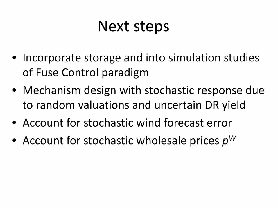
Next steps

• Incorporate storage and into simulation studies of Fuse Control paradigm

• Mechanism design with stochastic response due to random valuations and uncertain DR yield

• Account for stochastic wind forecast error • Account for stochastic wholesale prices pW