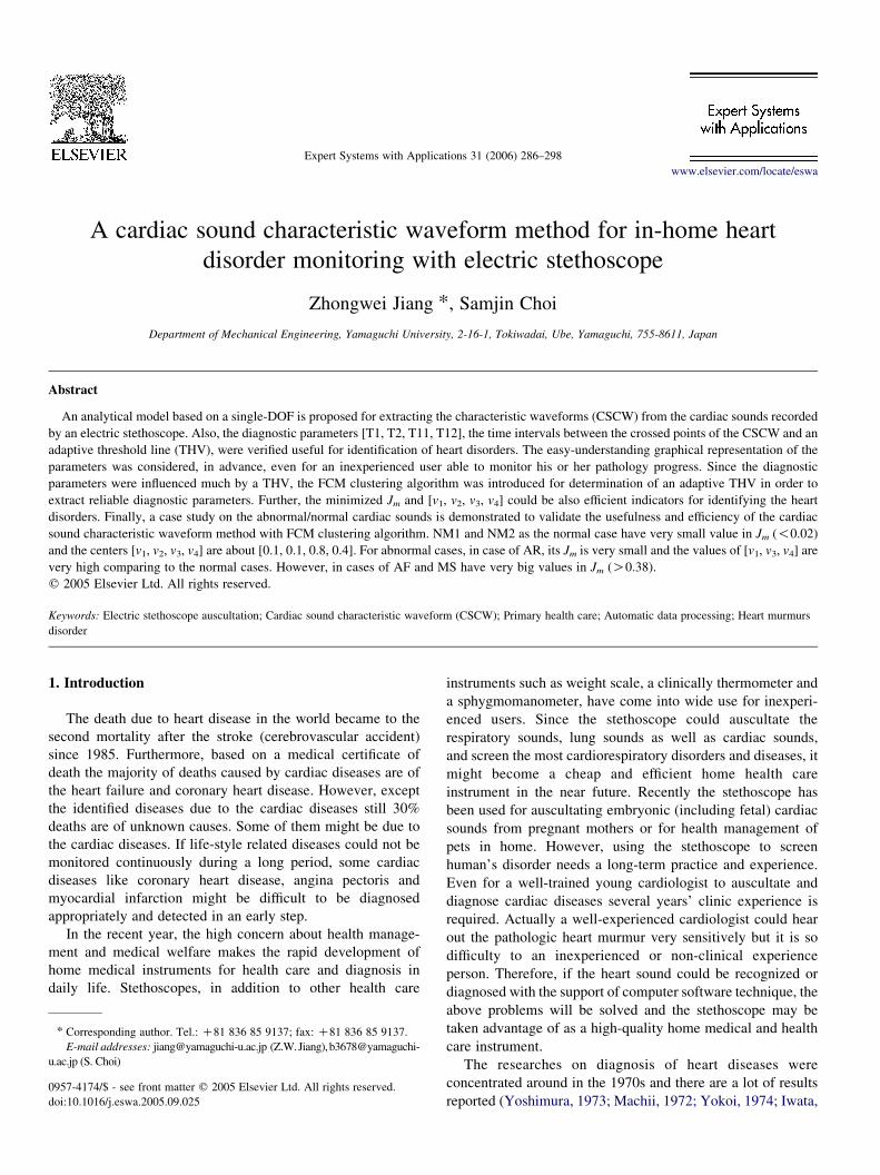
A cardiac sound characteristic waveform method for in-home heart

disorder monitoring with electric stethoscope

Zhongwei Jiang *, Samjin Choi

Department of Mechanical Engineering, Yamaguchi University, 2-16-1, Tokiwadai, Ube, Yamaguchi, 755-8611, Japan

Abstract

An analytical model based on a single-DOF is proposed for extracting the characteristic waveforms (CSCW) from the cardiac sounds recorded

by an electric stethoscope. Also, the diagnostic parameters [T1, T2, T11, T12], the time intervals between the crossed points of the CSCW and an

adaptive threshold line (THV), were verified useful for identification of heart disorders. The easy-understanding graphical representation of the

parameters was considered, in advance, even for an inexperienced user able to monitor his or her pathology progress. Since the diagnostic

parameters were influenced much by a THV, the FCM clustering algorithm was introduced for determination of an adaptive THV in order to

extract reliable diagnostic parameters. Further, the minimized Jm and [v1, v2, v3, v4] could be also efficient indicators for identifying the heart

disorders. Finally, a case study on the abnormal/normal cardiac sounds is demonstrated to validate the usefulness and efficiency of the cardiac

sound characteristic waveform method with FCM clustering algorithm. NM1 and NM2 as the normal case have very small value in Jm (!0.02)

and the centers [v1, v2, v3, v4] are about [0.1, 0.1, 0.8, 0.4]. For abnormal cases, in case of AR, its Jm is very small and the values of [v1, v3, v4] are

very high comparing to the normal cases. However, in cases of AF and MS have very big values in Jm (O0.38).

q 2005 Elsevier Ltd. All rights reserved.

Keywords: Electric stethoscope auscultation; Cardiac sound characteristic waveform (CSCW); Primary health care; Automatic data processing; Heart murmurs

disorder

1. Introduction

The death due to heart disease in the world became to the

second mortality after the stroke (cerebrovascular accident)

since 1985. Furthermore, based on a medical certificate of

death the majority of deaths caused by cardiac diseases are of

the heart failure and coronary heart disease. However, except

the identified diseases due to the cardiac diseases still 30%

deaths are of unknown causes. Some of them might be due to

the cardiac diseases. If life-style related diseases could not be

monitored continuously during a long period, some cardiac

diseases like coronary heart disease, angina pectoris and

myocardial infarction might be difficult to be diagnosed

appropriately and detected in an early step.

In the recent year, the high concern about health manage-

ment and medical welfare makes the rapid development of

home medical instruments for health care and diagnosis in

daily life. Stethoscopes, in addition to other health care

0957-4174/$ - see front matter q 2005 Elsevier Ltd. All rights reserved.

doi:10.1016/j.eswa.2005.09.025

* Corresponding author. Tel.: C81 836 85 9137; fax: C81 836 85 9137.

E-mail addresses: jiang@yamaguchi-u.ac.jp (Z.W.Jiang),b3678@yamaguchi-

u.ac.jp (S. Choi)

instruments such as weight scale, a clinically thermometer and

a sphygmomanometer, have come into wide use for inexperi-

enced users. Since the stethoscope could auscultate the

respiratory sounds, lung sounds as well as cardiac sounds,

and screen the most cardiorespiratory disorders and diseases, it

might become a cheap and efficient home health care

instrument in the near future. Recently the stethoscope has

been used for auscultating embryonic (including fetal) cardiac

sounds from pregnant mothers or for health management of

pets in home. However, using the stethoscope to screen

human’s disorder needs a long-term practice and experience.

Even for a well-trained young cardiologist to auscultate and

diagnose cardiac diseases several years’ clinic experience is

required. Actually a well-experienced cardiologist could hear

out the pathologic heart murmur very sensitively but it is so

difficulty to an inexperienced or non-clinical experience

person. Therefore, if the heart sound could be recognized or

diagnosed with the support of computer software technique, the

above problems will be solved and the stethoscope may be

taken advantage of as a high-quality home medical and health

care instrument.

The researches on diagnosis of heart diseases were

concentrated around in the 1970s and there are a lot of results

reported (Yoshimura, 1973; Machii, 1972; Yokoi, 1974; Iwata,

Expert Systems with Applications 31 (2006) 286–298

www.elsevier.com/locate/eswa

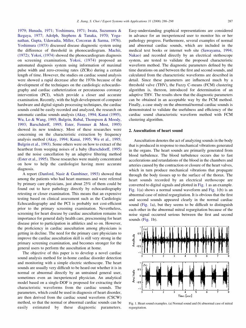
Fig. 1. Heart sound examples. (a) Normal sound and (b) abnormal case of mitral

regurgitation.

Z. Jiang, S. Choi / Expert Systems with Applications 31 (2006) 286–298 287

1979; Hunada, 1971; Yoshimura, 1971; Iwata, Suzumura &

Ikegaya, 1977; Adolph, Stephens & Tanaka, 1970; Yoga-

nathan, Gupta, Udawadia, Miller, Corcoran & Sarma, 1976).

Yoshimura (1973) discussed disease diagnostic system using

the difference of threshold in phonocardiogram. Machii,

(1972); Yokoi, (1974) showed the phonocardiogram diagnosis

on screening examination, Yokoi, (1974) proposed an

automated diagnosis system using information of maximal

pulse width and zero-crossing rates (ZCRs) during a certain

length of time. However, the studies on cardiac sound analysis

were showed a rapid decrease after the 1970s because of the

development of the techniques on the cardiologic echocardio-

graphy and cardiac catheterization or percutaneous coronary

intervention (PCI), which provide a closer and accurate

examination. Recently, with the high development of computer

hardware and digital signals processing techniques, the cardiac

sounds could be easily recorded and analyzed, the research on

automatic cardiac sounds analysis (Akay, 1994; Kanai (1995),

Wu, Lo & Wang, 1995; Bulgrin, Rubal, Thompson & Moody,

1993; Barschdorff, 1995; Ester, Femmer & Most, 1995)

showed its new tendency. Most of these researches were

concerning on the characteristic extraction by frequency

analysis method (Akay, 1994; Kanai, 1995; Wu et al., 1995;

Bulgrin et al., 1993). Some others were on how to extract of the

heartbeat from weeping noises of a baby (Barschdorff, 1995)

and the noise cancellation by an adaptive filtering method

(Ester et al., 1995). Those researches were mainly concentrated

on how to help the cardiologist having more accurate

diagnosis.

A report (Danford, Nasir & Gumbiner, 1993) showed that

among the patients who had heart murmurs and were referred

by primary care physicians, just about 25% of them could be

found out to have pathology directly by echocardiography

retesting or closer examination. This means that an expensive

testing based on clinical assessment such as the Cardiologic

Echocardiography and the PCI is probably not cost-efficient

prior to the primary screening examination. Nevertheless,

screening for heart disease by cardiac auscultation remains its

importance for general daily health care, prescreening for heart

disease prior to participation in athletics and so on. However,

the proficiency in cardiac auscultation among physicians is

getting in decline. The need for the primary care physicians to

improve the cardiac auscultation skill is still very strong in the

primary screening examination, and becomes stronger for the

general users to perform the auscultation at home.

The objective of this paper is to develop a novel cardiac

sound analysis method for in-home cardiac disorder detection

and monitoring with a simple electric stethoscope. The heart

sounds are usually very difficult to be heard out whether it is in

normal or abnormal directly by an untrained general user,

sometimes even an inexperienced physician. An analytical

model based on a single-DOF is proposed for extracting their

characteristic waveforms from the cardiac sounds. The

parameters, which could be used in diagnosis of heart disorder,

are then derived from the cardiac sound waveform (CSCW)

method, so that the normal or abnormal cardiac sounds can be

easily estimated by these diagnostic parameters.

Easy-understanding graphical representations are considered

in advance for an inexperienced user to monitor his or her

pathology progress. Furthermore, several examples of normal

and abnormal cardiac sounds, which are included in the

medical text books or internet web site (Sawayama, 1994;

Nakao) and recorded directly by an electrical stethoscope

system, are tested to validate the proposed characteristic

waveform method. The diagnostic parameters defined by the

time durations on and between the first and second sounds, and

calculated from the characteristic waveforms are described in

detail. Since these parameters are influenced much by a

threshold valve (THV), the Fuzzy C-means (FCM) clustering

algorithm is, thereon, introduced for determination of an

adaptive THV. The results show that the diagnostic parameters

can be obtained in an acceptable way by the FCM method.

Finally, a case study on the abnormal/normal cardiac sounds is

demonstrated to validate the usefulness and efficiency of the

cardiac sound characteristic waveform method with FCM

clustering algorithm.

2. Auscultation of heart sound

Auscultation denotes the act of analyzing sounds in the body

that is produced in response to mechanical vibrations generated

in the organs. The heart sounds are primarily generated from

blood turbulence. The blood turbulence occurs due to fast

accelerations and retardations of the blood in the chambers and

arteries caused by the contraction or closure of the heart valves,

which in turn produce mechanical vibrations that propagate

through the body tissues up to the surface of the thorax. The

heart sounds recorded by an electrical stethoscope are

converted to digital signals and plotted in Fig. 1 as an example.

Fig. 1(a) shows a normal sound waveform and Fig. 1(b) is an

abnormal case of mitral regurgitation. It is obvious that the first

and second sounds appeared clearly in the normal cardiac

sound (Fig. 1a), but they seems to be difficult to distinguish

each other in the abnormal mitral regurgitation because of the

noise signal occurred serious between the first and second

sounds (Fig. 1b).

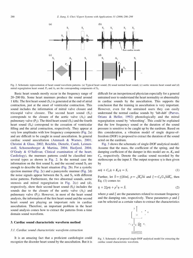
Fig. 2. Schematic representation of heart sound waveform patterns. (a) Typical heart sound, (b) usual normal heart sound, (c) aortic stenosis heart sound and (d)

mitral regurgitation heart sound. P2 and A2 are the corresponding components of S2.

Fig. 3. Schematic of proposed single-DOF analytical model for extracting the

cardiac sound characteristic waveform.

Z. Jiang, S. Choi / Expert Systems with Applications 31 (2006) 286–298288

Basic heart sounds mostly occur in the frequency range of

20–200 Hz. Some heart murmurs produce the sound around

1 kHz. The first heart sound (S1) is generated at the end of atrial

contraction, just at the onset of ventricular contraction. This

sound includes the information of mitral valve closure and

tricuspid valve closure. The second heart sound (S2)

corresponds to the closure of the aortic valve (A2) and

pulmonary valve (P2). The third heart sound (S3) and the fourth

heart sound (S4) correspond to the cessation of ventricular

filling and the atrial contraction, respectively. They appear at

very low amplitudes with low frequency components (Fig. 2a)

and are difficult to be caught in usual auscultation. In general

cardiac sound auscultation (Ammash & Warnes, 2001;

Christini & Glass, 2002; Reichlin, Dieterle, Camli, Leimen-

stoll, Schoenenberger & Martina, 2004; Hasfjord, 2004;

O’Grady & O’Sullivan; Clinical examination of the heart;

Cardiology), the murmurs patterns could be classified into

several types as shown in Fig. 2. In the normal case the

information on the first sound S1 and the second sound S2 are

enough to describe the heart situation (Fig. 2b). For a systolic

ejection murmur (Fig. 2c) and a pansystolic murmur (Fig. 2d)

the noise signals appear between the S1 and S2 with different

noise patterns. Furthermore, the two abnormal sounds, aortic

stenosis and mitral regurgitation in Fig. 2(c) and (d),

respectively, show their second heart sound (S2) includes the

sounds due to the closure of the aortic valve (A2) and

pulmonary valve (P2). However, in most of the heart sound

analysis, the information of the first heart sound and the second

heart sound are playing an important rule in cardiac

auscultation. Therefore, an important problem in the heart

sound analysis comes how to extract the patterns from a time

domain sound waveform.

3. Cardiac sound characteristic waveform method

3.1. Cardiac sound characteristic waveform extraction

It is an amazing fact that a proficient cardiologist could

recognize the disorder heart sound by the auscultation. But it is

difficult for an inexperienced physician especially for a general

untrained user to understand the heart normality or abnormality

in cardiac sounds by the auscultation. This supports the

conclusion that the training in auscultation is very important.

However, even for the untrained users they can easily

understand the normal cardiac sounds by ‘lub-dub’ (Purves,

Orians & Heller, 1992) phonologically and the mitral

regurgitation sound by ‘whooshing’. This could be explained

that the low frequency sound or the duration of the sound

pressure is sensitive to be caught up by the eardrum. Based on

this consideration, a vibration model of single degree-of-

freedom (DOF) is proposed to extract the duration of the sound

acted on the eardrum.

Fig. 3 shows the schematic of single-DOF analytical model.

Assume that the mass, the coefficient of the spring, and the

damping coefficient of the damper in this model are m, Kh and

Ch, respectively. Denote the cardiac sound recorded by the

stethoscope as the input S. The output response h is then given

by

m €hCCh _hCKhhZ S; (1)

Further, let �SZGjS=mj, pZffiffiffiffiffiffiffiffiffiffiKh=m

pand xZCh=2

ffiffiffiffiffiffiffiffiffimKh

p, then

Eq. (1) comes to:

€hC2xp _hCp2hZ �S: (2)

where p and x are the parameters related to resonant frequency

and the damping rate, respectively. These parameters p and x

can be selected as a certain values to extract the characteristics

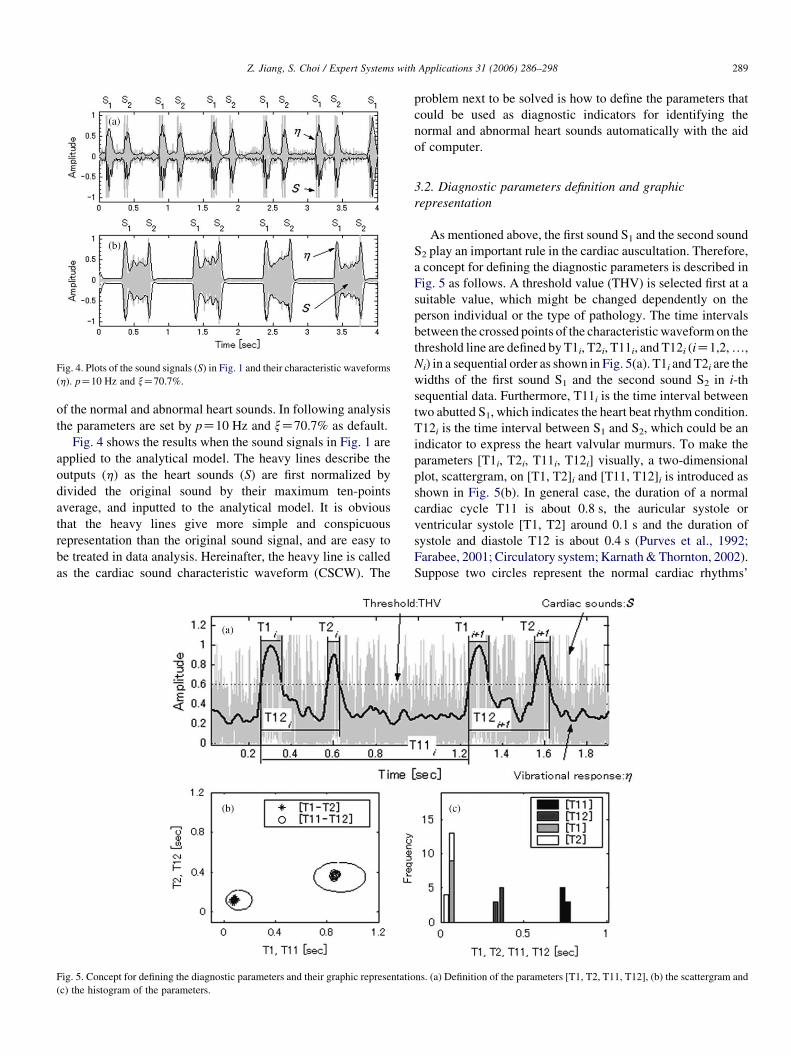
Fig. 4. Plots of the sound signals (S) in Fig. 1 and their characteristic waveforms

(h). pZ10 Hz and xZ70.7%.

Z. Jiang, S. Choi / Expert Systems with Applications 31 (2006) 286–298 289

of the normal and abnormal heart sounds. In following analysis

the parameters are set by pZ10 Hz and xZ70.7% as default.

Fig. 4 shows the results when the sound signals in Fig. 1 are

applied to the analytical model. The heavy lines describe the

outputs (h) as the heart sounds (S) are first normalized by

divided the original sound by their maximum ten-points

average, and inputted to the analytical model. It is obvious

that the heavy lines give more simple and conspicuous

representation than the original sound signal, and are easy to

be treated in data analysis. Hereinafter, the heavy line is called

as the cardiac sound characteristic waveform (CSCW). The

Fig. 5. Concept for defining the diagnostic parameters and their graphic representatio

(c) the histogram of the parameters.

problem next to be solved is how to define the parameters that

could be used as diagnostic indicators for identifying the

normal and abnormal heart sounds automatically with the aid

of computer.

3.2. Diagnostic parameters definition and graphic

representation

As mentioned above, the first sound S1 and the second sound

S2 play an important rule in the cardiac auscultation. Therefore,

a concept for defining the diagnostic parameters is described in

Fig. 5 as follows. A threshold value (THV) is selected first at a

suitable value, which might be changed dependently on the

person individual or the type of pathology. The time intervals

between the crossed points of the characteristicwaveformon the

threshold line are defined byT1i, T2i, T11i, and T12i (iZ1,2,.,

Ni) in a sequential order as shown in Fig. 5(a). T1i and T2i are the

widths of the first sound S1 and the second sound S2 in i-th

sequential data. Furthermore, T11i is the time interval between

two abutted S1, which indicates the heart beat rhythm condition.

T12i is the time interval between S1 and S2, which could be an

indicator to express the heart valvular murmurs. To make the

parameters [T1i, T2i, T11i, T12i] visually, a two-dimensional

plot, scattergram, on [T1, T2]i and [T11, T12]i is introduced as

shown in Fig. 5(b). In general case, the duration of a normal

cardiac cycle T11 is about 0.8 s, the auricular systole or

ventricular systole [T1, T2] around 0.1 s and the duration of

systole and diastole T12 is about 0.4 s (Purves et al., 1992;

Farabee, 2001; Circulatory system; Karnath&Thornton, 2002).

Suppose two circles represent the normal cardiac rhythms’

ns. (a) Definition of the parameters [T1, T2, T11, T12], (b) the scattergram and

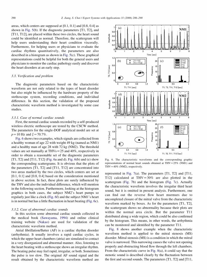
Fig. 6. The characteristic waveforms and the corresponding graphic

representations of normal heart sounds obtained at THVZ25% (NM1) and

THVZ40% (NM2), respectively.

Z. Jiang, S. Choi / Expert Systems with Applications 31 (2006) 286–298290

areas, which centers are supposed at [0.1, 0.1] and [0.8, 0.4] as

shown in Fig. 5(b). If the diagnostic parameters [T1, T2]i and

[T11, T12]i are placed within these two circles, the heart sound

could be identified as normal. Therefore, the scattergram will

help users understanding their heart condition viscerally.

Furthermore, for helping users or physicians to evaluate the

cardiac rhythms quantitatively, the parameters are also

described in a histogram as shown in Fig. 5(c). These graphical

representations could be helpful for both the general users and

physicians to monitor the cardiac pathology easily and discover

the heart disorders at an early step.

3.3. Verification and problem

The diagnostic parameters based on the characteristic

waveform are not only related to the types of heart disorder

but also might be influenced by the hardware property of the

stethoscope system, recording conditions, and individual

difference. In this section, the validation of the proposed

characteristic waveform method is investigated by some case

studies.

3.3.1. Case of normal cardiac sounds

First, the normal cardiac sounds recorded by a self-produced

wireless electric stethoscope are tested by the CSCW method.

The parameters for the single-DOF analytical model are set at

pZ10 Hz and xZ70.7%.

Fig. 6 shows two examples, which signals are collected from

a healthy woman of age 22 with weight 49 kg (named as NM1)

and a healthy man of age 28 with 72 kg (NM2). The threshold

values are set manually at THVsZ25 and 40%, respectively in

order to obtain a reasonable set of the diagnostic parameters

[T1, T2] and [T11, T12] (Fig. 6a and d). Fig. 6(b) and (e) show

the corresponding scattergrams. It is obvious that the plots of

the parameters [T1, T2] and [T11, T12] are concentrated into

two areas marked by the two circles, which centers are set at

[0.1, 0.1] and [0.8, 0.4] based on the consideration mentioned

in above section. In fact, these plots are surely influenced by

the THV and also the individual difference, which will mention

in the following section. Furthermore, looking at the histogram

graphics in both cases, the subject NM2’s heart pumps so

regularly just like a clock (Fig. 6f) and the subject NM1’s heart

is in normal but has a little fluctuation in heart beating (Fig. 6c).

3.3.2. Case of abnormal cardiac sounds

In this section some abnormal cardiac sounds collected in

the medical book (Sawayama, 1994) and online clinical

training website (Nakao) are used for validation of the

characteristic waveform method.

Atrial fibrillation/flutter (AF) is a cardiac rhythm disorder

(arrhythmia). It usually involves a rapid cardiac cycles, in

which the upper heart chambers (atria) are simulated to contact

in a very disorganized and abnormal manner. Also, listening to

the heart beating with a stethoscope shows an irregular rhythm.

The beating pulse may feel rapid, irregular, or both. Sometimes

the pulse is too slow. The original AF sound signal and the

result obtained by the characteristic waveform method are

represented in Fig. 7(a). The parameters [T1, T2] and [T11,

T12] calculated at THVZ30% are also plotted in the

scattergram (Fig. 7b) and the histogram (Fig. 7c). Actually

the characteristic waveform involves the irregular third heart

sound, but it is omitted in present analysis. Furthermore, one

can find out the reverse flow heart murmurs due to

uncompleted closure of the mitral valve from the characteristic

waveform marked by boxes. As for the parameters [T1, T2],

the scattergram shows no abnormality because their plots are

within the normal area circle. But the parameter T11

distributed along a wide region, which could be also confirmed

by the histogram. This means, in other words, the arrhythmia

can be monitored and identified by the parameter T11.

Fig. 8 shows another example when the characteristic

waveform method is applied to the mitral stenosis (MS)

disorder. Mitral stenosis (MS) is a condition in which the mitral

valve is narrowed. This narrowing causes the valve not opening

properly and obstructing blood flow through the left chambers.

From the characteristic curve in Fig. 8(a), it could say that the

stenotic sound is described clearly by the fluctuation between

the first and second sounds. The parameters [T1, T2] and [T11,

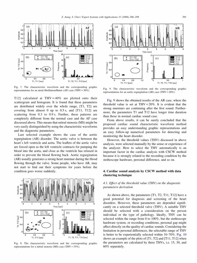
Fig. 7. The characteristic waveform and the corresponding graphic

representations for an atrial fibrillation/flutter (AF) case (THVZ30%).Fig. 9. The characteristic waveform and the corresponding graphic

representations for an aortic regurgitation (AR) case (THVZ20%).

Z. Jiang, S. Choi / Expert Systems with Applications 31 (2006) 286–298 291

T12] calculated at THVZ40% are plotted onto their

scattergram and histogram. It is found that these parameters

are distributed widely over the whole range, [T1, T2] are

covering from almost 0 up to 0.5 s, and [T11, T12] are

scattering from 0.3 to 0.9 s. Further, these patterns are

completely different from the normal case and the AF case

discussed above. This means that mitral stenosis (MS) might be

very easily distinguished by using the characteristic waveforms

and the diagnostic parameters.

Last selected example shows the case of the aortic

regurgitation (AR) disorder. The aortic valve is between the

heart’s left ventricle and aorta. The leaflets of the aortic valve

are forced open as the left ventricle contracts for pumping the

blood into the aorta, and close as the ventricle has relaxed in

order to prevent the blood flowing back. Aortic regurgitation

(AR) usually generates a strong heart murmur during the blood

flowing through the valve. Some people, who have AR, may

not start to find out their symptoms for years before the

condition goes worse suddenly.

Fig. 8. The characteristic waveform and the corresponding graphic

representations for a mitral stenosis (MS) case (THVZ35%).

Fig. 9 shows the obtained results of the AR case, where the

threshold value is set at THVZ20%. It is evident that the

strong murmurs are continuing after the first sound. Further-

more, the parameters T1 and T12 have longer time duration

than those in normal cardiac sound case.

From above results, it can be surely concluded that the

proposed cardiac sound characteristic waveform method

provides an easy understanding graphic representations and

an easy follow-up numerical parameters for detecting and

monitoring the heart disorder.

However, the threshold values (THV) discussed in above

analysis, were selected manually by the sense or experience of

the analyzer. How to select the THV automatically is an

important factor in the cardiac analysis with CSCW method

because it is strongly related to the recording condition by the

stethoscope hardware, personal difference, and so on.

4. Cardiac sound analysis by CSCW method with data

clustering technique

4.1. Effect of the threshold value (THV) on the diagnostic

parameters derivation

As shown above, the parameters [T1, T2, T11, T12] have a

good potential for diagnosis and screening of the heart

disorders. However, these parameters are depended signifi-

cantly on a selected threshold valve (THV). A suitable THV

should be selected with a consideration on the person

individual or the type of pathology. Ideally, THV can be

selected within the range from 0 to 100%, but the stethoscope

hardware system, or recording conditions, personal gap might

affect directly on the quality of cardiac sounds. Considering the

limitation in personal differences, the selectable range of THV

is better to be experientially selected within 10–70%. Fig. 10

shows an example of the plots of [T1, T2] and [T11, T12] when

the parameters are calculated by three THVs, i.e. 15, 30, and

60% separately.

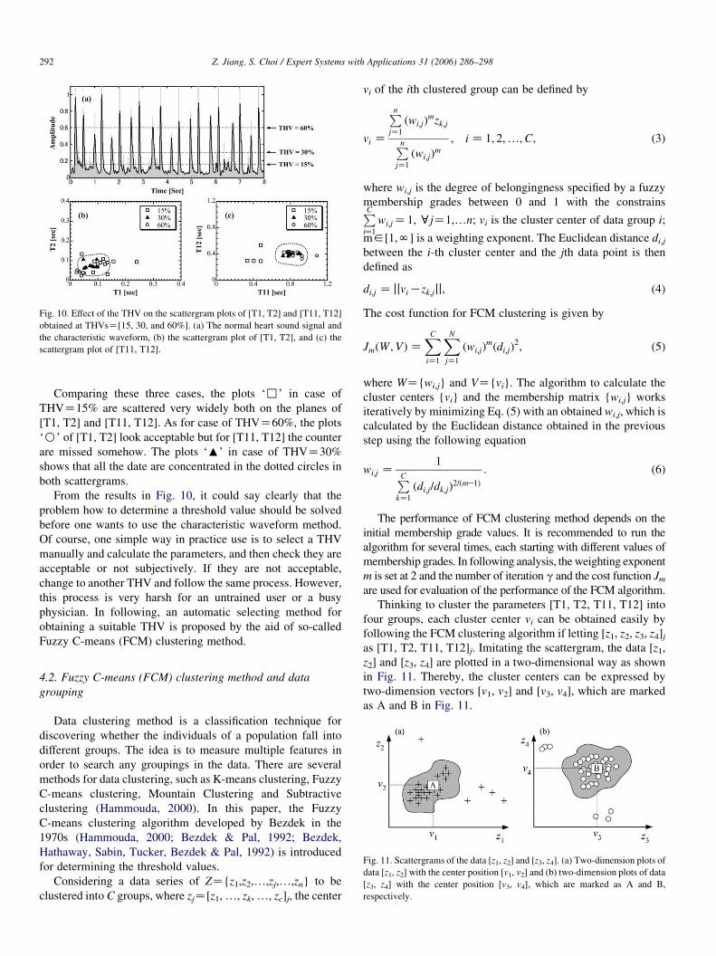
Fig. 10. Effect of the THV on the scattergram plots of [T1, T2] and [T11, T12]

obtained at THVsZ[15, 30, and 60%]. (a) The normal heart sound signal and

the characteristic waveform, (b) the scattergram plot of [T1, T2], and (c) the

scattergram plot of [T11, T12].

Z. Jiang, S. Choi / Expert Systems with Applications 31 (2006) 286–298292

Comparing these three cases, the plots ‘,’ in case of

THVZ15% are scattered very widely both on the planes of

[T1, T2] and [T11, T12]. As for case of THVZ60%, the plots

‘B’ of [T1, T2] look acceptable but for [T11, T12] the counter

are missed somehow. The plots ‘:’ in case of THVZ30%

shows that all the date are concentrated in the dotted circles in

both scattergrams.

From the results in Fig. 10, it could say clearly that the

problem how to determine a threshold value should be solved

before one wants to use the characteristic waveform method.

Of course, one simple way in practice use is to select a THV

manually and calculate the parameters, and then check they are

acceptable or not subjectively. If they are not acceptable,

change to another THV and follow the same process. However,

this process is very harsh for an untrained user or a busy

physician. In following, an automatic selecting method for

obtaining a suitable THV is proposed by the aid of so-called

Fuzzy C-means (FCM) clustering method.

Fig. 11. Scattergrams of the data [z1, z2] and [z3, z4]. (a) Two-dimension plots of

data [z1, z2] with the center position [v1, v2] and (b) two-dimension plots of data

[z3, z4] with the center position [v3, v4], which are marked as A and B,

respectively.

4.2. Fuzzy C-means (FCM) clustering method and data

grouping

Data clustering method is a classification technique for

discovering whether the individuals of a population fall into

different groups. The idea is to measure multiple features in

order to search any groupings in the data. There are several

methods for data clustering, such as K-means clustering, Fuzzy

C-means clustering, Mountain Clustering and Subtractive

clustering (Hammouda, 2000). In this paper, the Fuzzy

C-means clustering algorithm developed by Bezdek in the

1970s (Hammouda, 2000; Bezdek & Pal, 1992; Bezdek,

Hathaway, Sabin, Tucker, Bezdek & Pal, 1992) is introduced

for determining the threshold values.

Considering a data series of ZZ{z1,z2,.,zj,.,zn} to be

clustered into C groups, where zjZ[z1,., zk,., zc]j, the center

vi of the ith clustered group can be defined by

vi Z

Pn

jZ1

ðwi;jÞmzk;j

Pn

jZ1

ðwi;jÞm

; i Z 1; 2;.;C; (3)

where wi,j is the degree of belongingness specified by a fuzzy

membership grades between 0 and 1 with the constrainsPCiZ1

wi;jZ1, cjZ1,.n; vi is the cluster center of data group i;

m2[1,N] is a weighting exponent. The Euclidean distance di,j

between the i-th cluster center and the jth data point is then

defined as

di;j Z jjviKzk;jjj; (4)

The cost function for FCM clustering is given by

JmðW ;VÞZXC

iZ1

XN

jZ1

ðwi;jÞmðdi;jÞ

2; (5)

where WZ{wi,j} and VZ{vi}. The algorithm to calculate the

cluster centers {vi} and the membership matrix {wi,j} works

iteratively by minimizing Eq. (5) with an obtained wi,j, which is

calculated by the Euclidean distance obtained in the previous

step using the following equation

wi;j Z1

PCkZ1

ðdi;j=dk;jÞ2=ðmK1Þ

: (6)

The performance of FCM clustering method depends on the

initial membership grade values. It is recommended to run the

algorithm for several times, each starting with different values of

membership grades. In following analysis, the weighting exponent

m is set at 2 and the number of iteration g and the cost function Jm

are used for evaluation of the performance of the FCM algorithm.

Thinking to cluster the parameters [T1, T2, T11, T12] into

four groups, each cluster center vi can be obtained easily by

following the FCM clustering algorithm if letting [z1, z2, z3, z4]jas [T1, T2, T11, T12]j. Imitating the scattergram, the data [z1,

z2] and [z3, z4] are plotted in a two-dimensional way as shown

in Fig. 11. Thereby, the cluster centers can be expressed by

two-dimension vectors [v1, v2] and [v3, v4], which are marked

as A and B in Fig. 11.

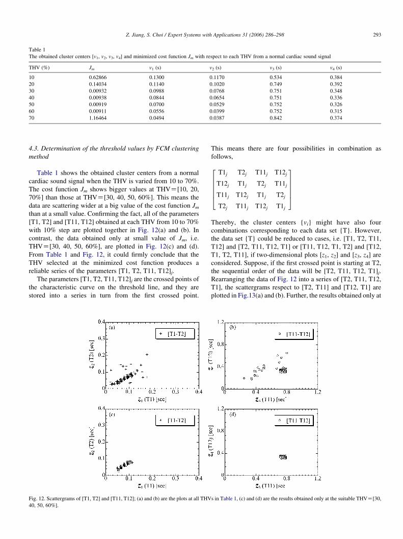
Table 1

The obtained cluster centers [v1, v2, v3, v4] and minimized cost function Jm with respect to each THV from a normal cardiac sound signal

THV (%) Jm v1 (s) v2 (s) v3 (s) v4 (s)

10 0.62866 0.1300 0.1170 0.534 0.384

20 0.14034 0.1140 0.1020 0.749 0.392

30 0.00932 0.0988 0.0768 0.751 0.348

40 0.00938 0.0844 0.0654 0.751 0.336

50 0.00919 0.0700 0.0529 0.752 0.326

60 0.00911 0.0556 0.0399 0.752 0.315

70 1.16464 0.0494 0.0387 0.842 0.374

Z. Jiang, S. Choi / Expert Systems with Applications 31 (2006) 286–298 293

4.3. Determination of the threshold values by FCM clustering

method

Table 1 shows the obtained cluster centers from a normal

cardiac sound signal when the THV is varied from 10 to 70%.

The cost function Jm shows bigger values at THVZ[10, 20,

70%] than those at THVZ[30, 40, 50, 60%]. This means the

data are scattering wider at a big value of the cost function Jm

than at a small value. Confirming the fact, all of the parameters

[T1, T2] and [T11, T12] obtained at each THV from 10 to 70%

with 10% step are plotted together in Fig. 12(a) and (b). In

contrast, the data obtained only at small value of Jm, i.e.

THVZ[30, 40, 50, 60%], are plotted in Fig. 12(c) and (d).

From Table 1 and Fig. 12, it could firmly conclude that the

THV selected at the minimized cost function produces a

reliable series of the parameters [T1, T2, T11, T12]j.

The parameters [T1, T2, T11, T12]j are the crossed points of

the characteristic curve on the threshold line, and they are

stored into a series in turn from the first crossed point.

Fig. 12. Scattergrams of [T1, T2] and [T11, T12]; (a) and (b) are the plots at all THV

40, 50, 60%].

This means there are four possibilities in combination as

follows,

T1j T2j T11j T12j

T12j T1j T2j T11j

T11j T12j T1j T2j

T2j T11j T12j T1j

266664

377775

Thereby, the cluster centers {vi} might have also four

combinations corresponding to each data set {T}. However,

the data set {T} could be reduced to cases, i.e. [T1, T2, T11,

T12] and [T2, T11, T12, T1] or [T11, T12, T1, T2] and [T12,

T1, T2, T11], if two-dimensional plots [z1, z2] and [z3, z4] are

considered. Suppose, if the first crossed point is starting at T2,

the sequential order of the data will be [T2, T11, T12, T1]j.

Rearranging the data of Fig. 12 into a series of [T2, T11, T12,

T1], the scattergrams respect to [T2, T11] and [T12, T1] are

plotted in Fig.13(a) and (b). Further, the results obtained only at

s in Table 1, (c) and (d) are the results obtained only at the suitable THVZ[30,

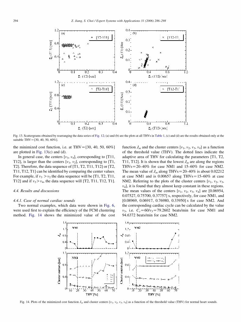
Fig. 13. Scattergrams obtained by rearranging the data series of Fig. 12; (a) and (b) are the plots at all THVs in Table 1, (c) and (d) are the results obtained only at the

suitable THVZ[30, 40, 50, 60%].

Z. Jiang, S. Choi / Expert Systems with Applications 31 (2006) 286–298294

the minimized cost function, i.e. at THVZ[30, 40, 50, 60%]

are plotted in Fig. 13(c) and (d).

In general case, the centers [v3, v4], corresponding to [T11,

T12], is larger than the centers [v1, v2], corresponding to [T1,

T2]. Therefore, the data sequence of [T1, T2, T11, T12] or [T2,

T11, T12, T1] can be identified by comparing the center values.For example, if v3 Ov2 the data sequence will be [T1, T2, T11,

T12] and if v2Ov4, the data sequence will [T2, T11, T12, T1].

4.4. Results and discussions

4.4.1. Case of normal cardiac sounds

Two normal examples, which data were shown in Fig. 6,

were used first to explain the efficiency of the FCM clustering

method. Fig. 14 shows the minimized value of the cost

Fig. 14. Plots of the minimized cost function Jm and cluster centers [v1, v2, v3

function Jm and the cluster centers [v1, v2, v3, v4] as a function

of the threshold value (THV). The dotted lines indicate the

adaptive area of THV for calculating the parameters [T1, T2,

T11, T12]. It is shown that the lowest Jm are along the regions

THVsZ20–40% for case NM1 and 15–60% for case NM2.

The mean value of Jm along THVsZ20–40% is about 0.02212

at case NM1 and is 0.00657 along THVsZ15–60% at case

NM2. Referring to the plots of the cluster centers [v1, v2, v3,

v4], it is found that they almost keep constant in these regions.

The mean values of the centers [v1, v2, v3, v4] are [0.06954,

0.07527, 0.75700, 0.37757] s, respectively, for case NM1, and

[0.08969, 0.06917, 0.76980, 0.33950] s for case NM2. And

the corresponding cardiac cycle can be calculated by the value

v3, i.e. CyZ60/v3Z79.2602 beats/min for case NM1 and

94.6372 beats/min for case NM2.

, v4] as a function of the threshold value (THV) for normal heart sounds.

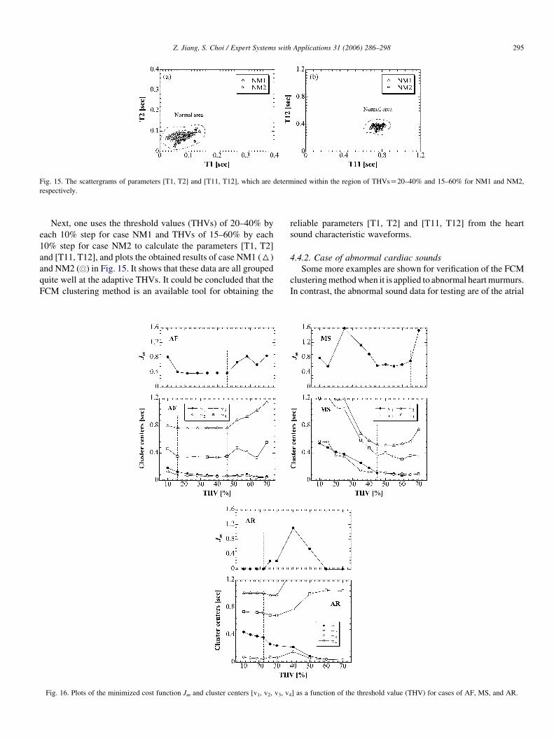
Fig. 15. The scattergrams of parameters [T1, T2] and [T11, T12], which are determined within the region of THVsZ20–40% and 15–60% for NM1 and NM2,

respectively.

Z. Jiang, S. Choi / Expert Systems with Applications 31 (2006) 286–298 295

Next, one uses the threshold values (THVs) of 20–40% by

each 10% step for case NM1 and THVs of 15–60% by each

10% step for case NM2 to calculate the parameters [T1, T2]

and [T11, T12], and plots the obtained results of case NM1 (6)

and NM2 ( ) in Fig. 15. It shows that these data are all grouped

quite well at the adaptive THVs. It could be concluded that the

FCM clustering method is an available tool for obtaining the

Fig. 16. Plots of the minimized cost function Jm and cluster centers [v1, v2, v3, v

reliable parameters [T1, T2] and [T11, T12] from the heart

sound characteristic waveforms.

4.4.2. Case of abnormal cardiac sounds

Some more examples are shown for verification of the FCM

clusteringmethodwhen it is applied to abnormal heartmurmurs.

In contrast, the abnormal sound data for testing are of the atrial

4] as a function of the threshold value (THV) for cases of AF, MS, and AR.

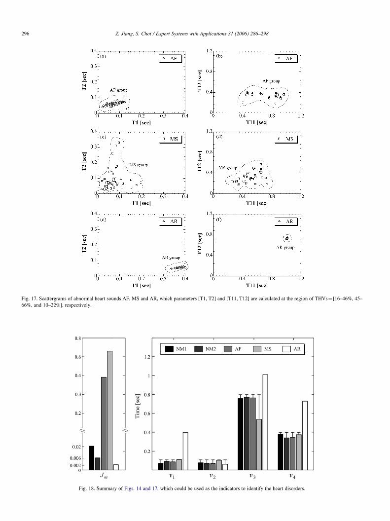
Fig. 17. Scattergrams of abnormal heart sounds AF, MS and AR, which parameters [T1, T2] and [T11, T12] are calculated at the region of THVsZ[16–46%, 45–

66%, and 10–22%], respectively.

Fig. 18. Summary of Figs. 14 and 17, which could be used as the indicators to identify the heart disorders.

Z. Jiang, S. Choi / Expert Systems with Applications 31 (2006) 286–298296

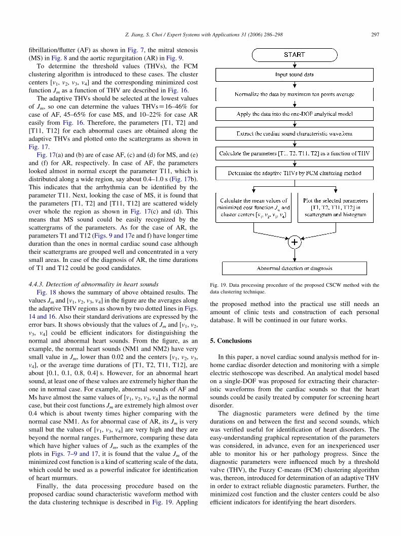
Fig. 19. Data processing procedure of the proposed CSCW method with the

data clustering technique.

Z. Jiang, S. Choi / Expert Systems with Applications 31 (2006) 286–298 297

fibrillation/flutter (AF) as shown in Fig. 7, the mitral stenosis

(MS) in Fig. 8 and the aortic regurgitation (AR) in Fig. 9.

To determine the threshold values (THVs), the FCM

clustering algorithm is introduced to these cases. The cluster

centers [v1, v2, v3, v4] and the corresponding minimized cost

function Jm as a function of THV are described in Fig. 16.

The adaptive THVs should be selected at the lowest values

of Jm, so one can determine the values THVsZ16–46% for

case of AF, 45–65% for case MS, and 10–22% for case AR

easily from Fig. 16. Therefore, the parameters [T1, T2] and

[T11, T12] for each abnormal cases are obtained along the

adaptive THVs and plotted onto the scattergrams as shown in

Fig. 17.

Fig. 17(a) and (b) are of case AF, (c) and (d) for MS, and (e)

and (f) for AR, respectively. In case of AF, the parameters

looked almost in normal except the parameter T11, which is

distributed along a wide region, say about 0.4–1.0 s (Fig. 17b).

This indicates that the arrhythmia can be identified by the

parameter T11. Next, looking the case of MS, it is found that

the parameters [T1, T2] and [T11, T12] are scattered widely

over whole the region as shown in Fig. 17(c) and (d). This

means that MS sound could be easily recognized by the

scattergrams of the parameters. As for the case of AR, the

parameters T1 and T12 (Figs. 9 and 17e and f) have longer time

duration than the ones in normal cardiac sound case although

their scattergrams are grouped well and concentrated in a very

small areas. In case of the diagnosis of AR, the time durations

of T1 and T12 could be good candidates.

4.4.3. Detection of abnormality in heart sounds

Fig. 18 shows the summary of above obtained results. The

values Jm and [v1, v2, v3, v4] in the figure are the averages along

the adaptive THV regions as shown by two dotted lines in Figs.

14 and 16. Also their standard derivations are expressed by the

error bars. It shows obviously that the values of Jm and [v1, v2,

v3, v4] could be efficient indicators for distinguishing the

normal and abnormal heart sounds. From the figure, as an

example, the normal heart sounds (NM1 and NM2) have very

small value in Jm, lower than 0.02 and the centers [v1, v2, v3,

v4], or the average time durations of [T1, T2, T11, T12], are

about [0.1, 0.1, 0.8, 0.4] s. However, for an abnormal heart

sound, at least one of these values are extremely higher than the

one in normal case. For example, abnormal sounds of AF and

Ms have almost the same values of [v1, v2, v3, v4] as the normal

case, but their cost functions Jm are extremely high almost over

0.4 which is about twenty times higher comparing with the

normal case NM1. As for abnormal case of AR, its Jm is very

small but the values of [v1, v3, v4] are very high and they are

beyond the normal ranges. Furthermore, comparing these data

which have higher values of Jm, such as the examples of the

plots in Figs. 7–9 and 17, it is found that the value Jm of the

minimized cost function is a kind of scattering scale of the data,

which could be used as a powerful indicator for identification

of heart murmurs.

Finally, the data processing procedure based on the

proposed cardiac sound characteristic waveform method with

the data clustering technique is described in Fig. 19. Appling

the proposed method into the practical use still needs an

amount of clinic tests and construction of each personal

database. It will be continued in our future works.

5. Conclusions

In this paper, a novel cardiac sound analysis method for in-

home cardiac disorder detection and monitoring with a simple

electric stethoscope was described. An analytical model based

on a single-DOF was proposed for extracting their character-

istic waveforms from the cardiac sounds so that the heart

sounds could be easily treated by computer for screening heart

disorder.

The diagnostic parameters were defined by the time

durations on and between the first and second sounds, which

was verified useful for identification of heart disorders. The

easy-understanding graphical representation of the parameters

was considered, in advance, even for an inexperienced user

able to monitor his or her pathology progress. Since the

diagnostic parameters were influenced much by a threshold

valve (THV), the Fuzzy C-means (FCM) clustering algorithm

was, thereon, introduced for determination of an adaptive THV

in order to extract reliable diagnostic parameters. Further, the

minimized cost function and the cluster centers could be also

efficient indicators for identifying the heart disorders.

Z. Jiang, S. Choi / Expert Systems with Applications 31 (2006) 286–298298

Finally, a case study on the abnormal/normal cardiac sounds

is demonstrated to validate the usefulness and efficiency of the

cardiac sound characteristic waveform method with FCM

clustering algorithm.

References

Adolph, R. J., Stephens, J. F., & Tanaka, K. (1970). The clinical value of

frequency analysis of the first heart sound in myocardial infarction.

Circulation XLI, 41, 1003–1014.

Akay, M. (1994). Automated noninvasive detection of coronary artery disease

using wavelet-based neural networks. Intelligent Engineering System

Artificial Neural Network, 14, 517–522.

Ammash, N. M., & Warnes, C. A. (2001). Ventricular septal defects in adults.

American College of Physicians–American Society of Internal Medicine,

135, 812–824.

Barschdorff, D. (1995). Phonocardiogram signal analysis in infants based on

wavelet transformsandartificial neuralnetworks.Processing Annual Science

Meeting Computer Cardiologic, 753–756.

Bezdek, J. C., Hathaway, R. J., Sabin, M. J., & Tucker, W. T. (1992). In J. C.

Bezdek, & S. K. Pal (Eds.), Fuzzy methods for pattern recognition (pp.

138–142). New York: IEEE Press.

Bezdek, J. C., & Pal, S. K. (1992). Fuzzy models for pattern recognition. New

York: IEEE Press.

Bulgrin, J. R., Rubal, B. J., Thompson, C. R., & Moody, J. M. (1993).

Comparison of short-time fourier, wavelet and time-domain analyses of

intracardiac sounds. Biomedical Sciences Instrumentation, 29, 465–472.

Cardiology. Available at: http://rjmatthewsmd.com/

Christini, D. J., & Glass, L. (2002). Mapping and control of complex cardiac

arrhythmias. Chaos, 12, 732–739.

Circulatory system. Available at: http://www.cyber-north.com/anatomy/circu-

lat.htm

Clinical examination of the heart. Available at: http://www.cuhk.edu.hk/cslc/

materials/pclm1011/pclm1011.html

Danford, D. A., Nasir, A., & Gumbiner, C. (1993). Cost assessment of the

evaluation of heart murmurs in children. Pediatrics, 91, 365–368.

Ester, S., Femmer, U., & Most, E. (1995). Heart sound analysis utilizing

adaptive filter technique and neural networks. Techisches Messen, 62(3),

107–112.

Farabee, M. J. (2001). The circulatory system. Available at: http://www.emc.

maricopa.edu/faculty/farabee/BIOBK/BioBookcircSYS.html

Hammouda, K. (2000). A comparative study of data clustering techniques.

SYDE 625: Tools of intelligent systems design, course project.

Hasfjord, F. (2004). Heart sound analysis with time dependent fractal

dimensions. Sweden: Linkopings University.

Hunada, T. (1971). The extraction of phonocardiogram parameter by digital

processing. Rinsho Phonocardiogram, 1, 9–18 (in Japan).

Iwata, A. (1979). Automated identification of phonocardiogram: Processing by

linear predictive coding method. Japanese Journal of Medical Electronics

and Biological Engineering, 17, 185–192 (in Japan).

Iwata, A., Suzumura, N., & Ikegaya, K. (1977). Pattern classification of the

phonocardiogram using linear prediction analysis. Medical and Biological

Engineering and Computing, 15(4), 407–412.

Kanai, H. (1995). A time-varing AR modeling of heart wall vibration.

Processing IEEE International Conference on Acoustic Speech Signal

Processing, 2, 941–944.

Karnath, B., & Thornton, W. (2002). Auscultation of the heart. Hospital

Physician, 39–43.

Machii, K. (1972). The problems on phonocardiogram diagnosis equipment,

cardiac sound diagnosis equipment for mass screening or automatic cardiac

sound diagnosis. Sogo-Rinsho, 21, 695–699 (in Japan).

Nakao, K. Online bed side learning: Heart sound auscultation. Available at

http://www.medic.mie-u.ac.jp/student/sinnzou.html

O’Grady, M. R., & O’Sullivan, M. L. Clinical cardiology concepts. Available

at: http://www.vetgo.com/cardio/concepts/concsect.php?conceptkeyZ29

Purves, W. K., Orians, G. H., & Heller, H. C. (1992). Life: The science of

biology (4th ed.). Sunderland, MA: Sinauer Associates Inc./WH Freeman.

Reichlin, S., Dieterle, T., Camli, C., Leimenstoll, B., Schoenenberger, R. A., &

Martina, B. (2004). Initial clinical evaluation of cardiac systolic murmurs in

the ED by noncardiologists. American Journal of Emergency Medicine,

22(2), 71–75.

Sawayama, T. (1994). Auscultation training by CD: Heart sound. Japan:

Nankodo (in Japan).

Wu, C. H., Lo, C. W., & Wang, J. F. (1995). Computer-aided analysis and

classification of heart sounds based on neural networks and time analysis.

Processing IEEE International Conference Acoustic Speech Signal

Processing , 3455–3458.

Yoganathan, A. P., Gupta, R., Udawadia, F. E., Miller, J. W., Corcoran, W. H.,

Sarma, R., et al. (1976). Use of the fast fourier transform for the frequency

analysis of the first heart sound in normal man. Medical and Biological

Engineering and Computing, 14(1), 49–73.

Yokoi, S., et al. (1974). Automatic phonocardiogram diagnosis equipment:

Application on screening system. Sogo-Rinsho, 23, 180–188 (in Japan).

Yoshimura, M. (1971). Automatic phonocardiogram management equipment.

Rinsho Phonocardiogram, 1, 1–7 (in Japan).

Yoshimura, T., et al. (1973). The applied formal phonocardiogram of the

computer in medical care. Sogo-Rinsho, 22, 40–46 (in Japan).