A Case Study in Collocation: Heat Transfer Effects inCavitation Bubble Dynamics

Matthew WarnezFaculty advisor: Eric Johnsen

2012 December 19

Contents

1 Introduction 1

2 Physical problem 22.1 Governing equations . . . . . . . . . . . . . . . . . . . . . . . . . . . . . . . . . . . . 22.2 Change of variables . . . . . . . . . . . . . . . . . . . . . . . . . . . . . . . . . . . . . 2

3 Collocation method 33.1 Chebyshev polynomial expansions . . . . . . . . . . . . . . . . . . . . . . . . . . . . . 43.2 Implementation . . . . . . . . . . . . . . . . . . . . . . . . . . . . . . . . . . . . . . . 6

4 Results 84.1 Periodic forcing . . . . . . . . . . . . . . . . . . . . . . . . . . . . . . . . . . . . . . . 84.2 Gaussian bump . . . . . . . . . . . . . . . . . . . . . . . . . . . . . . . . . . . . . . . 11

5 Conclusions 125.1 Future work . . . . . . . . . . . . . . . . . . . . . . . . . . . . . . . . . . . . . . . . . 12

6 Appendix 13

7 References 13

1 Introduction

Rapid fluctuations of pressure and temperature are common inside a cavitating bubble, but modelingthe full temperature distribution inside the bubble creates a host of numerical challenges. In thisstudy we will use a collocation method to solve the equations of cavitation bubble dynamics withonly very few assumptions. These assumptions, namely uniform pressure inside the bubble and aspherical symmetry, allow use of the well-known Rayleigh-Plesset equation, but aim to have minimallydeleterious effects on accuracy.

Collocation is a numerical method that can be used to solve partial differential equations. Byexpanding an unknown function into a linear combination of basis functions and evaluating this

1

function at a number of points in the domain, the weights of the basis functions can be solved forat each time step. The temperature distribution inside the bubble wall makes a good candidate forcollocation.

2 Physical problem

2.1 Governing equations

The radial dynamics of the bubble are governed by Keller’s equation, a variant of the Rayleigh-Plessetequation which accounts for effects of compressibility.(

1− R

cL

)RR +

3

2

(1− R

3cL

)R2 =

1

ρL

(1 +

R

cL+R

cL

d

dt

)[pB − pA] (1)

R is the bubble radius, cL is the sound speed in the surrounding liquid, ρL is the liquid density, pB isthe liquid pressure at the bubble wall, pA is the far-field (ambient) pressure. Here, overdots denotederivatives with respect to time. The pressure inside the bubble, p, taken to be uniform throughout,is described by

p =3

R

((γ − 1)λ

∂T

∂r

∣∣∣∣R

− γpR)

(2)

where λ(T ) is the thermal conductivity, T is the temperature, r is the distance from the bubble’scenter, and γ is the ratio of specific heats. The external pressure pB is related to the internal pressureby a stress balance at the bubble’s center, which gives

p = pB +2S

R+

4µLR

R(3)

where S is the surface tension, and µL is the liquid viscosity. The temperature and the thermalconductivity inside the bubble is allowed to vary over space, and is governed by the equation

γ

γ − 1

p

T

[∂T

∂t+

1

γp

((1− γ)λ

∂T

∂r− rp

3

)∂T

∂r

]− p = ∇ · (λ∇T ) (4)

We make the “cold” liquid assumption

T (R, t) = T∞ (5)

that is, the bubble temperature at the bubble wall is fixed at the ambient liquid temperature, T∞. Ithas been repeatedly shown that this is a reasonable approximation for liquids in the vicinity of roomtemperature.

2.2 Change of variables

We introduce the auxiliary variable

τ =

∫ T

T∞

λ(T ′)dT ′ (6)

2

so that

∇ · (λ∇T ) = ∇ ·(λ∂T

∂τ

∂τ

∂r

)= ∇ ·

(λ

1

λ

∂τ

∂r

)= ∇2τ (7)

To approximate the dependence of thermal conductivity on temperature we use the linear relation

λ(T ) = AT +B (8)

where A = 5.528 · 10−5 J/m s K2 and B = 1.165 · 10−2 J/m s K. This allows inversion of the definitionof τ to find

T =√λ2∞ + 2Aτ − B

A(9)

where λ∞ = AT∞ +B.Furthermore, we use the coordinate

x =r

R(10)

to fix the domain for spatial discretization. In all that follows, x = 0 hence refers to the bubble center,while x = 1 refers to the bubble wall.

3 Collocation method

To solve for the temperature-like distribution τ over space and time, we use a collocation method.In this method, τ is expanded into a partial sum of time-dependent coefficients an(t) multiplied intobasis functions φn(y):

τ(t, y) =N∑n=0

an(t)φn(x) (11)

The goal is to, at every time step, solve for the time-dependent coefficients such that τ accuratelyapproximates the temperature-like distribution inside the bubble. We can write that

∂τ

∂t=

N∑n=0

an(t)φn(x) = f

(x,R, p, p,

∂τ

∂x,∂2τ

∂x2

)(12)

where the nonlinear function f results from equation (4) after the appropriate change in variables. Byevaluating (12) at N + 1 collocation points, a system of N + 1 equations for the unknown collocationcoefficients a0, . . . , aN is created.

If the basis functions φn(x) are chosen properly, then helpful expressions for the spatial-derivativesof τ can be extracted.

3

3.1 Chebyshev polynomial expansions

In this study, we will use the even Chebyshev polynomials of the first kind, T2n(x), as the basisfunctions. In what follows, we will derive all of the relations necessary to make effective use of theChebyshev polynomials for collocation.

The Chebyshev polynomials are well known to abide by the derivative recurrence relation

2Tn =1

n+ 1

dTn+1

dx− 1

n− 1

dTn−1dx

(13)

which can be alternatively written and expanded as

d

dxTn+1 = 2(n+ 1)Tn +

n+ 1

n− 1

d

dxTn−1 (14)

d

dxT2n = 2(2n)T2n−1 +

2n

2n− 2

d

dxT2n−2 (15)

= 2(2n)T2n−1 +2n

2n− 2

(2(2n− 2)T2n−3 +

2n− 2

2n− 4

d

dxT2n−4

)(16)

= 2(2n)T2n−1 + 2(2n)T2n−3 +2n

2n− 4

d

dxT2n−4 (17)

= 2(2n)T2n−1 + 2(2n)T2n−3 + · · ·+ 2(2n)T1 + (2n)d

dxT0 (18)

= 4nn∑k=1

T2k−1 (19)

since dT0/dx = 0. This can be used to express the first spatial derivative of τ as a linear combinationof the an coefficients.

dτ

dx=

N∑n=0

andT2ndx

(20)

=N∑n=0

an

(4n

n∑k=1

T2k−1

)(21)

=N∑n=1

enT2n−1 (22)

where

en = 4N∑k=n

kak (23)

4

Now from the original recurrence relation we consider that

dT2n−1dx

= 2(2n− 1)T2n−2 +2n− 1

2n− 3

dT2n−3dx

(24)

= 2(2n− 1)T2n−2 +2n− 1

2n− 3

(2(2n− 3)T2n−4 +

2n− 3

2n− 5

dT2n−5dx

)(25)

= 2(2n− 1)T2n−2 + 2(2n− 1)T2n−4 + · · ·+ 2(2n− 1)T2 + (2n− 1)dT1dx

(26)

= 2(2n− 1)T2n−2 + 2(2n− 1)T2n−4 + · · ·+ 2(2n− 1)T2 + (2n− 1)T0 (27)

= (2n− 1)n∑k=1

fkT2(k−1) (28)

where

fk =

{1 if k = 1

2 if k 6= 1(29)

This allows us to write the second derivate of an even Chebyshev polynomial as

d2T2ndx2

= 4nn∑k=1

dT2k−1dx

(30)

= 4nn∑k=1

((2k − 1)

k∑m=1

fmT2(m−1)

)(31)

= 4nn∑k=1

ck,nT2(k−1) (32)

where

ck,n = fk

n∑m=k

(2m− 1) (33)

The second derivate of τ(t, y) can be written

∂2τ

∂x2=

N∑n=1

endT2n−1dx

(34)

=N∑n=1

dnT2n−2 (35)

where

dn = fn

N∑k=n

(2k − 1)ek (36)

In a similar way it can be shown that

d3T2ndx3

= 16nn∑k=2

(n∑

m=k

cm,n(m− 1)

)T2n−3 n = 2, 3, . . . (37)

5

and that

∂3T2n∂x3

=N∑n=1

dndT2n−2dx

(38)

=N∑n=1

dn

(4(n− 1)

n−1∑k=1

T2k−1

)(39)

=N∑n=2

4dn(n− 1)n∑k=2

T2k−3 (40)

=N∑n=2

gnT2n−3 (41)

where

gn =N∑k=n

4dk(k − 1) (42)

(43)

3.2 Implementation

At some time t, let τ (t) be a vector in which each component is the temperature-like variable τevaluated at a unique collocation point. To avoid Runge’s phenomenon, we use the collocation pointsgiven by the Gauss-Lobatto quadrature points

xk = cosπk

2N, k = 0, 1, . . . , N (44)

giving

τ =

τ(t, x0)τ(t, x1)

...τ(t, xN)

(45)

Now if we let A be the collocation matrix defined by

A =

T0(x0) T2(x0) · · · T2N(x0)T0(x1) T2(x1) · · · T2N(x1)

......

. . ....

T0(xN) T2(xN) · · · T2N(xN)

(46)

and a(t) be the coefficient vector

a =

a0(t)a1(t)

...aN(t)

(47)

6

then

τ = Aa (48)

Note that the entries in A can easily be computed from the Chebyshev polynomial property that

T2n(ym) = cos (2n arccos ym) (49)

To compute the first spatial derivative of τ we define

B =

T1(y0) T3(x0) · · · T2N−1(x0)T1(x1) T3(x1) · · · T2N−1(x1)

......

. . ....

T1(xN) T3(xN) · · · T2N−1(xN)

(50)

and note that from equation (23)

en = 4[0 · · · 0 n n+ 1 · · · N

]

a0a1...

an−1anan+1

...aN

(51)

Therefore

e =

e1e2e3...eN

= 4

0 1 2 3 · · · N0 0 2 3 · · · N0 0 0 3 · · · N...

......

.... . .

...0 0 0 0 · · · N

a0a1a2a3...aN

(52)

Defining the matrix in (51) to be E/4, the value of ∂τ/∂y at each collocation point is given by

∂τ

∂y= BEa (53)

By a similar process, a matrix D generated from the values of dn given in equation (36) allows thesecond derivative to be written

∂2τ

∂y2= ADa (54)

In fact, any spatial derivative of τ can be written as a linear transformation on the coefficients vectora. In the appendix we give the matrices E and D for the N = 6 case.

7

Equations (48), (53), and (54) reduce equation (12) to

Aa = f (x, R, p, p, BEa, ADa) (55)

where x = [x0, x1, . . . , xN ]>. To satisfy the boundary condition (5), which corresponds to∑N

n=0 anT2n(x0) =0, we replace the first element of f with 0.

Given some initial condition a0, this system of ordinary differential equations, along with equations(1) and (2), can now be solved and stepped forward in time to find any later a. This was done byusing MATLAB’s ode45 solver along with MATLAB’s left division of A into f at every timestep.

To convert the collocation coeffients into a temperature distribution we use τ = Aa and thenevaluate (9).

4 Results

4.1 Periodic forcing

In this section we set the ambient pressure to oscillate so as to drive the bubble. That is, we let

pA(t) = p∞ (1− ε sinωt) (56)

where P∞ is the static pressure, ε is a dimensionless quantity that controls the amplitude of thepressure waves, and ω is the angular frequency.

In what follows we take the initial radius of the bubble to be R0 = 10µm and the initial bubblewall velocity to be R0 = 0. We let the initial temperature inside the bubble be uniform at T∞,which corresponds to the collocation coefficient vector a0 = 0. The other properties used wereω = 3.91 ·105 s−1, γ = 1.4, cL = 1490 m/s, µL = 7.98 ·10−4 Pa s, ρL = 997 kg/m2, S = 7.12 ·10−2 N/m,p∞ = 101325 Pa, and T∞ = 300 K. In figures 1, 2, and 3, the results for the N = 6 case are shown.In figure 4, a finer resolution of the temperature distribution was made by letting N = 16.

0 5 10 150.2

0.4

0.6

0.8

1

1.2

1.4

1.6

1.8

t

R/R

0

Bubble radiusAmbient pressure

Figure 1: Bubble radius versus time for a pressure amplitude ε = 0.8. The ambient pressure functionis overlaid in dashed lines.

8

0 5 10 150

1

2

3

4

5

6

7

t

P/P

0

Internal pressure

Figure 2: Internal bubble pressure versus time for the case in Figure 1.

Figure 3: The temperature distribution versus time for the setup of Figures 1 and 2. The number ofcollocation points used was N + 1 = 6 + 1.

9

Figure 4: The temperature distribution versus time for the setup of Figures 1 and 2, but with N = 16.

It is worthwhile to compare these results to the polytropic approach in which the temperature inthe bubble is taken to be uniform and the bubble pressure is described by

p =

(p∞ +

2S

R

)(R0

R

)3γ

(57)

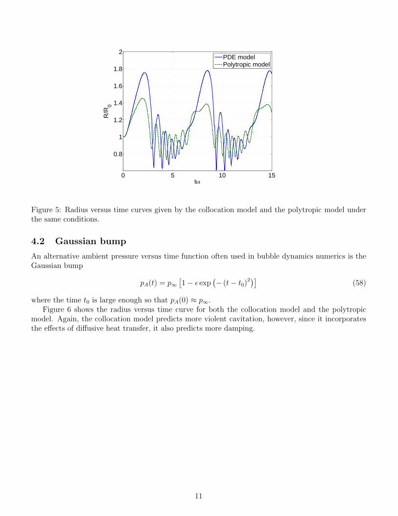
Figure 5 shows the striking difference between the two models, which has been previously observed byProsperetti (1988). It verifies Prosperetti’s result that the PDE model predicts more violent cavitation- larger maximum radii and smaller minimum radii.

10

0 5 10 15

0.8

1

1.2

1.4

1.6

1.8

2

t

R/R

0

PDE modelPolytropic model

Figure 5: Radius versus time curves given by the collocation model and the polytropic model underthe same conditions.

4.2 Gaussian bump

An alternative ambient pressure versus time function often used in bubble dynamics numerics is theGaussian bump

pA(t) = p∞[1− ε exp

(− (t− t0)2

)](58)

where the time t0 is large enough so that pA(0) ≈ p∞.Figure 6 shows the radius versus time curve for both the collocation model and the polytropic

model. Again, the collocation model predicts more violent cavitation, however, since it incorporatesthe effects of diffusive heat transfer, it also predicts more damping.

11

0 5 10 150

0.2

0.4

0.6

0.8

1

1.2

1.4

1.6

1.8

t

R/R

0

PDE modelPolytropic modelAmbient pressure

Figure 6: Radius versus time curves given by the collocation model and the polytropic model underthe influence of a Gaussian pressure drop. The form of the pressure drop is overlaid.

5 Conclusions

This work serves as a successful application of the principals of collocation to bubble dynamics. Thebenefits of the use of the Chebyshev polynomials were formally shown, and an efficient matrix algebraimplementation was derived. The computational results affirm several of the conclusions made byprevious authors in the field, in particular, that models that account for thermal behavior give vastlydifferent results than the simpler polytropic model.

5.1 Future work

A collocation method can also be used to solve for the temperature distribution in the liquid. Whereasin this study we made the cold liquid approximation, in reality the liquid temperature TL is governedby

∂T

∂t+R2R

r2∂TL∂r

= DL∇2TL (59)

where DL is the liquid thermal diffusivity. By using the coordinate transformation

ξ =l

r/R− 1 + l(60)

where l is a measure of the thermal diffusion length, the domain [R,∞) is projected onto [0, 1]. Asseen previously, the domain [0, 1] lends itself easily to collocation through the Chebyshev polynomials.

Another area of future work is to apply these methods to solve bubble dynamics equations thatmodel the effects of nonlinear viscoelasticity. Solving these equations involves integrating over theshear stress field in the surrounding viscoelastic medium. Just as recurrence relations for the Cheby-shev polynomials allowed easy computation of derivatives, the same may be so for integration.

12

6 Appendix

For the N = 6 case, the matrices is equations (53) and (54) are

E =

0 4 8 12 16 20 240 0 8 12 16 20 240 0 0 12 16 20 240 0 0 0 16 20 240 0 0 0 0 20 240 0 0 0 0 0 24

(61)

D =

0 4 32 108 256 500 8640 0 48 192 480 960 16800 0 0 120 384 840 15360 0 0 0 224 640 12960 0 0 0 0 360 6900 0 0 0 0 0 5280 0 0 0 0 0 0

(62)

7 References

• V. Kamath and A. Prosperetti, “Numerical integration methods in gas-bubble dynamics,” J.Acoust. Soc. Am. 85, 1538-1548 (1989).

• A. Prosperetti, L. Crum, and K. Commander, “Nonlinear bubble dynamics” J. Acoust. Soc. Am.83, 502 (1988).

• L. Stricker and A. Prosperetti, “Validation of an approximate model for the thermal behavior inacoustically driven bubbles,” J. Acoust. Soc. Am. 130, 3243-3251 (2011).

13