A CASE STUDY OF ONION PRODUCTION IN THE TIPAJARA WATERSHED, MIZQUE BOLIVIA

By

FRANKLYN B. ARAGONA

submitted in partial fulfillment of the requirements for the degree of

MASTER OF SCIENCE IN FORESTRY

MICHIGAN TECHNOLOGICAL UNIVERSITY

2003

i

The thesis: “A Case Study of Onion Production in the Tipajara Watershed, Mizque

Bolivia” is hereby approved in partial fulfillment of the requirements for the Degree

of MASTER OF SCIENCE IN FORESTRY.

School of Forest Resources and Environmental Sciences Signatures:

Thesis Advisor:__________________________ Blair Orr Dean:__________________________________

Glenn D. Mroz Date:__________________________________

ii

The geologists, the earth’s scientists, have given us a beautiful and elaborate picture of the planet’s formation and development; they have constructed a time scheme with which they can diagram, as with an overlay, each evolutionary step in the long process. But all that, I maintain, is merely information. It is not knowledge; even less is it understanding. Knowledge and understanding, though based on information as an essential component, require more, namely, feeling, intuition, physical contact—touching, and sympathy, and love. It is possible for a man and woman to know and understand one another, in this complete sense. It is possible to know, though to lesser degree, other living things—birds, animals, plants. It is even possible to know, through love, a place, a certain landscape, a river, canyon, mesa, mountain. From Abbey’s Road by Edward Abbey

My Thesis as an Onion (Variedad Mizqueño)

Once upon a time there was a peasant woman and a very wicked woman she was. And she died and did not leave a single good deed behind. The devils caught her and plunged her into the lake of fire. So her guardian angel stood and wondered what good deed of hers he could remember to tell to God; 'She once pulled up an onion in her garden,' said he, 'and gave it to a beggar woman.' And God answered: 'You take that onion then, hold it out to her in the lake, and let her take hold and be pulled out. And if you can pull her out of the lake, let her come to Paradise, but if the onion breaks, then the woman must stay where she is.' The angel ran to the woman and held out the onion to her. 'Come,' said he, 'catch hold and I'll pull you out.' He began cautiously pulling her out. He had just pulled her right out, when the other sinners in the lake, seeing how she was being drawn out, began catching hold of her so as to be pulled out with her. But she was a very wicked woman and she began kicking them. 'I'm to be pulled out, not you. It's my onion, not yours.' As soon as she said that, the onion broke. And the woman fell into the lake and she is burning there to this day. So the angel wept and went away.

From The Brothers Karamazov by Fyodor Dostoevsky

iii

TABLE OF CONTENTS LIST OF FIGURES…………………………….……………………………. v LIST OF TABLES…………………………………………………………… vii ACKNOWLEDGEMENTS………………………………………………… . viii CHAPTER I INTRODUCTION…………………………………………… 1 CHAPTER II STUDY OBJECTIVES…………………………………….… 3 CHAPTER III COUNTRY BACKGROUND……………………………… 4 CHAPTER IV STUDY AREA BACKGROUND…………………………… 18 CHAPTER V METHODS AND DATA ……………………………………. 33 CHAPTER VI RESULTS AND DISCUSSION FOR TENURE AND LAND USE…………..……………………………………………………………… 46 CHAPTER VII ONIONS………………………………………………………. 68 CHAPTER VIII RESULTS AND DISCUSSION FOR ONION PRODUCTION 90 CHAPTER IX CONCLUSIONS AND RECOMMENDATIONS …………… 112 LITERATURE CITED…………………………………..……………………. 118 APPENDICES……………………………………………...…………………. 121

iv

LIST OF FIGURES FIGURE 3.1 MAP OF SOUTH AMERICA …………………………………………5 FIGURE 3.2 THE NINE DEPARTMENTS OF BOLIVA…………………………...6 FIGURE 4.1 TIPAJARA WATERSHED DELINEATION AND DRAINAGE……19 FIGURE 4.2 DISCHARGE OF WATER, TIPAJARA RIVER………………….... 18 FIGURE 4.3 PHOTO OF TIPAJARA WATERSHED...………..…………………..20 FIGURE 4.4 WATER BALANCE TIPAJARA WATERSHED……………………21 FIGURE 4.5 TEMPERATURE CATEGORIES TIPAJARA WATERSHED…….. 22 FIGURE 4.6 SOIL SERIES BY SUBGROUP IN THE TIPJARA WATERSHED…..…………………………………………………………………...24 FIGURE 4.7 NUTRITIONAL STATE OF CHILDREN UNDER FIVE YEARS, TIPA TIPA………………………………………………………………………...…25 FIGURE 4.8. PRE-COLOMBIAN ZOOMORPHIC FIGURES NEAR THE TOWN OF MIZQUE………….………………………………………………………..…….26 FIGURE 4.9 COLONIAL BRIDGE BETWEEN MIZQUE & COCHABAMBA….28 FIGURE 4.10 THE CATHEDRAL IN MIZQUE…..……………………………….29 FIGURE 5.1 STUDY COMMUNITIES BY NUMBER…………………………….39 FIGURE 6.1 TRADITIONAL CORN SILOS……………………………………….48 FIGURE 6.2 A TRADITIONAL BAND IN TIPA TIPA……………………………49 FIGURE 6.3 LAND TENURE AND INFRASTRUCTURE, TIPA TIPA 1961…....54 FIGURE 6.4 GALERIA FILTRANTE, TIPA TIPA………………………………...58 FIGURE 6.5 IRRIGATION CANAL, TIPA TIPA………………………………….58 FIGURE 6.6 INFRASTRUCTURE TIPA TIPA 2002………………………………60 FIGURE 6.7 LAND USE AND LAND COVER, TIPA TIPA 1961………………..62 FIGURE 6.8 LAND USE AND LAND COVER, TIPA TIPA 2002………………..64 FIGURE 6.9 ERODED HILLSIDE LANDS, TIPA TIPA…………………………..65 FIGURE 7.1 ONION SEEDBED IN TIPA TIPA…...………………………………71 FIGURE 7.2. CHICKEN MANURE………………………………………………...72 FIGURE 7.3 THE YUNTA…………………………………………………………...73 FIGURE 7.4. TRANSPLATING ONIONS………………………………………….74 FIGURE 7.5. THE THAMIDA……………………………………………………….75 FIGURE 7.6 HARVESTING ONIONS………………………..……………………76 FIGURE 7.7. THE PRIMARY INPUTS FOR ONION PRODUCTION……………78 FIGURE 7.8 ONION PLANT TISSUE DAMANGED BY MILDEW AND LEAF BLIGHT……………………………………...………………………………………80 FIGURE 7.9. ONION CROP AT THE ONSET OF A CLADOSPORIUM ATTACK…………………………………………………………….……………....81 FIGURE 7.10. TYPICAL LESIONS OF ALTERNARIA…………………………....82 FIGURE 7.11 THE MARKET DISTRIBUTION NETWORK FOR ONIONS…….87 FIGURE 8.1 IRRIGATED CROPS , TIPA TIPA JULY 2002……………………...91 FIGURE 8.2 INCOME LINES FOR YIELD OF 15 TN/HA……………………....101 FIGURE 8.3 INCOME LINES FOR YIELD OF 20 TN/HA………………………102 FIGURE 8.4 INCOME LINES FOR YIELD OF 25 TN/HA………………………102 FIGURE 8.5 INCOME LINES FOR YIELD OF 30 TN/HA………………………103

v

FIGURE 8.6 RESULTS OF TUKEY TEST FOR DIFFERENCE IN USE OF TOTAL LABOR BY PARCEL SIZE CLASS……………………………………..104 FIGURE 8.7 RESULTS OF TUKEY TEST FOR DIFFERENCE IN USE OF OXEN BY PARCEL SIZE CLASS………………………………………………...104 FIGURE 8.8 RESULTS OF TUKEY TEST FOR DIFFERENCE IN USE OF SEED BY PARCEL SIZE CLASS…………………………………………………104 FIGURE 8.9 RESULTS OF TUKEY TEST FOR DIFFERENCE IN USE OF N BY PARCEL SIZE CLASS……………………………………………………...105 FIGURE 8.10 RESULTS OF TUKEY TEST FOR DIFFERENCE IN PRODUCTION COST BY PARCEL SIZE CLASS……………………………….105 FIGURE 8.11 RESULTS OF TUKEY TEST FOR DIFFERENCE IN YIELD BY PARCEL SIZE CLASS…………………………………………………………….105 FIGURE 8.12 CURING ONIONS IN THE FIELD………………………………..106 FIGURE 8.13 CURING ONIONS IN BURLAP BAGS………………………...…107 FIGURE 8.14 PLASTIC SACKS TO IMPROVE MARKETING………………....108 FIGURE 8.15 ONION CROP BEING DESTROYED BY DISEASE……………..111

vi

LIST OF TABLES TABLE 3.1 CENSUS DATA BY GENDER AND AREA FOR 1950, 1976, 1992, &2001…………………………………………………………………………………8 TABLE 3.2 POPULATION DENSITY BY DEPARTMENT 1992 & 2001 CENSUS……………………………………………………………………………....9 TABLE 4.1 USDA SOILS ORDERS AND GROUPS FOR THE TIPAJARA WATERSHED……………………………………………………………………….22 TABLE 4.2 CHARACTERISTICS AND DISTRIBUTION OF DOMINANT SOIL SUBGROUPS IN THE TIPAJARA WATERSHED…….………………………….23 TABLE 5.1 SAMPLE SIZE BY COMMUNITY……………………………………38 TABLE 5.2 PHYSICAL INPUTS FOR ONION PRODUCTION IN THE TIPAJARA WATERSHED…………………………………………………….……43 TABLE 5.3 ECONOMIC INPUTS FOR ONION PRODUCTION IN THE TIPAJARA WATERSHED………………….……………………………………....43 TABLE 5.4 ECONOMIC INDICATORS FOR ONION PRODUCTION IN THE TIPAJARA WATERSHED………………………………………………………….43 TABLE 5.5 DEMOGRAPHIC AVERAGES PER HOUSEHOLD IN THE TIPAJARA WATERSHED…………………………………………………...……..44 TABLE 5.6 MEAN NUMBER OF ANIMALS PER HOUSEHOLD IN THE TIPAJARA WATERSHED………………………………………………………….44 TABLE 6.1 LAND TENURE ANALYSIS AND LAND DISTRIBUTION FOR 1961, 2002, AND FUTURE GENERATIONS……………...………………………57 TABLE 8.1. PEARSON CORRELATION COEFFICIENTS NOT INCLUDED IN REGRESSION MODEL…………………………………………………………..…93 TABLE 8.2 VARIABLES FOR ONION YIELD REGRESSION…………………. 94 TABLE 8.3 PEARSON CORRELATION COEFFICIENTS FOR VARIABLES INCLUDED IN REGRESSION MODEL………………………………………...…94 TABLE 8.4 REGRESSION MODEL FOR LOSING FARMERS…………………..97 TABLE 8.5 REGRESSION MODEL FOR WINNING FARMERS………………..97 TABLE 8.6 PARCEL SIZE CLASSES FOR TUKEY TEST……………………...103 TABLE 8.7 PRICE PER BAG AND # OF FARMERS APPLYING IMPROVED MARKETING TECHNOLOGY BY SIZE CLASS ONIONS, TIPAJARA WATERSHED…………………………………………………………………...…109

vii

ACKNOWLEDGEMENTS

I am grateful and fortunate to have had the opportunity to work with my advisor Blair Orr. His constant support and guidance greatly contributed to the quality of this work. Blair’s tireless effort to assist Peace Corps students in the field is a direct benefit to those that most require his assistance: poor families in developing countries. He is an inspiration to us all. I would like to thank the members of my graduate committee: Brad Baltensperger, David Flaspohler, and Casey Huckins. I am also thankful for Anne Maclean’s help with the GIS and image processing required for this project. Thank you friends and family for supporting and assisting me as I traipse around the world. Special thanks to my mother and father. Quiero agradecer a la comunidad de Tipa Tipa, por su apoyo en mis trabajos y por hacerme sentir como un miembro de la comunidad. Agradecimientos a Toribio Maygua y Mario Huanca por sus trabajos, por lo que caminaron tanto en el sol he podido realizar el estudio. Extiendo mis sinceros agradecimientos a los miembros del Comité Agropecuario de Tipa Tipa: Moisés Jiménez, Wilfredo Claros, y Noel Castro. Ellos me apoyaron en todo y me hicieron sentir como un hermano. Por fin, le agradezco a Don Filiberto Rojas, compartía sus conocimientos con todo gusto, y siempre me trataba con cariño y respeto.

viii

CHAPTER I: INTRODUCTION

In August of 2000, I arrived in the city of Cochabamba, Bolivia to begin my

two-year service as a Peace Corps volunteer (PCV). After three months of technical

and language training, I was assigned to a small rural village in the Province of

Mizque called Tipa Tipa. My job description was vague, but encouraging, as I was

sent to help farmers with soil and water conservation.

As a Peace Corps volunteer in rural Bolivia, it was my job to be an agent of

change. The more I interacted with local people, however, the more I realized how

little I really did know about the farm systems that their livelihoods depend upon.

Ultimately, I had to address the fundamental questions of change in development.

Why change? Why should they change? Perhaps there is no reason to change. Of

course I realized that the people were, by and large, poor, but I wasn’t quite

convinced that change would necessarily eliminate this.

In Tipa Tipa, onions were everywhere. They were unavoidable. The people

seemed almost obsessed with them. So I began by working long, hard days in the

onion fields, learning the ins and outs of production, becoming familiar with the

farmers’ personalities and their approach to agriculture. I did a little of everything:

potato harvests, sowing maize, plowing fields, and, of course, working onions. Of all

the hard labor that I did, nothing was more exhausting or more backbreaking than

onions. I must have started off with a bias against the thankless task of onion farming

from the very beginning.

Yet the more I interacted with local people, the more I realized that their

affinity for onions was purely economic. Onion farming did have a past history of

1

success and profitability. The first seed of doubt germinated in June of 2001, when

disease began to attack onion crops, and the farmers responded by fumigating with

tenacity and despair, at the expense, I might add, of their own health. At the request

of several farmers, I brought samples of the diseased plant tissue to the nearby city of

Sucre, where Dr. Walter Kaiser, plant pathologist and Peace Corps volunteer, had a

laboratory for identifying plant diseases. Dr. Kaiser’s response was simple: crop

rotation. When I mentioned rotation to the farmers in Tipa Tipa, their response was

equally simple: laughter.

And so the process had begun. I was determined to ascertain why the farmers

were so attached to onion farming. I was hardly in a position to suggest changing the

entire cropping system without first understanding the dynamics of onion production.

And still, the specter of change hung over me. I must have believed in change. I

must have gone to Bolivia with a whole arsenal of American beliefs and ideals:

change is progress and progress is wealth and wealth is good. The farmers, of course,

also believed that wealth is good, it just seemed hopelessly unattainable for most of

them.

But more than just convincing farmers of the need for change, perhaps I was

most interested in convincing myself. So I studied onions. I labored over them,

thought about them in the evenings as I ate them with my meals. I even brought my

girlfriend a sack of onions as a gift. And yes, as time passed, I became convinced of

the need for change. And perhaps in the process I might have convinced a couple of

farmers that change might not be a bad idea.

2

CHAPTER II: STUDY OBJECTIVES In this study I use several different methodologies to describe the farm system

in the Tipajara watershed in the Mizque province of Cochabamba, Bolivia. It was my

goal to provide a thorough description of the farm system in the Tipajara watershed.

By combining GIS technology and ethnographic information, I explain changes and

trends in the farm system through time. This provides the necessary background for

understanding a very important component of irrigated agriculture in the area: onion

production. I use a statistical model generated from household survey data to analyze

the social and economic ramifications of an onion monoculture, and further

demonstrate that several virulent crop diseases have seriously compromised the onion

farmer’s ability to earn money. The possibilities of improved marketing for onions

are also discussed. I conclude by providing a list of recommendations for improving

farm system productivity and sustainability in the Tipajara watershed.

3

CHAPTER III: COUNTRY BACKGROUND

GEOGRAPHY

Bolivia is situated in the heart of the Andes mountains, at 17 00 S 65 00 W.

It is a country of geographic extremes, with alpine peaks reaching as high as 6,542

meters and lowland tropical rainforest at 100 m. The country has a total land area of

1,098,580 sq. km (CIA 2003). Bolivia is divided into three distinct ecological zones,

all of which correspond to extreme changes in elevation. The altiplano begins just

north of Lake Titicaca and stretches south for 800 km. at an average altitude of 4,000

meters. East of the altiplano lies the Cordillera Oriental, a broken stretch of

mountainous peaks and valleys from 4,250 m to just 100 m above sea level. Most

temperate valleys can be found here, at an average altitude of 2,500 m (Klein 1992).

Further east the mountains level off into the seemingly endless green sea of the

Amazon basin. Though the Amazon River itself does not flow through Bolivia, the

country is host to several major tributaries, the Beni and the Mamore being amongst

the largest. Historically, the altiplano has supported the largest human populations.

Bolivian land is 20 percent arid or desert, 40 percent rain forest, 25 percent

pasture and meadow, 2 percent arable, 2 percent inland water, and 11 percent other, a

very small percentage of which is irrigated (Hudson and Handratty 1989).

4

Figure 3.1: Map of South America (CIA 2003)

5

Bolivia is divided into nine departments: Beni, Chuquisaca, Cochabamba, La Paz,

Oruro, Pando, Potosi, Santa Cruz, and Tarija (Figure 3.2). Each department is further

divided into provinces.

Figure 3.2: The nine departments of Bolivia (IGM 2002)

6

POLITICS

Politically, Bolivia is a republic, with the seat of government located in the

altiplano city of La Paz. The president of the republic holds executive power. He is

elected once every four years by a majority popular vote. The number of political

parties in Bolivia and the fractious nature of Bolivian politics usually means that no

candidate wins a majority vote, in which case alliances between political parties are

formed and a vote in the National Congress determines which of the top three

candidates becomes president. Legislative power belongs to a bicameral Congress,

which consists of a Chamber of Deputies and a Senate (Hudson and Handratty 1989).

Though officially a republic since it declared independence from the Spanish crown

in 1825, Bolivia has been plagued by military coups, presidential assassinations, and

social unrest. The most recent example of which occurred in October of 2003, when

the president of Bolivia, Gonzalo Sanchez de Lozada, was forced to flee the country

in the wake of massive violent protests and repeated calls for his ouster. Sanchez de

Lozada was replaced by vice-president Carlos Mesa, who now presides as head of

state (Caceras 2003).

Currently, Bolivia’s most pressing political problems stem from the illicit

cultivation of coca for the production and export of cocaine. Under strong pressure

from the United States to eradicate illegal coca production, the Bolivian government

has had enormous difficulties with disruptive peasant populations whose economic

means of subsistence have been drastically altered by forced eradication. Sanchez de

Lozada argued that it was this segment of the Bolivian population that forced him to

resign the presidency (Caceras 2003).

7

DEMOGRAPHICS

The total population of Bolivia is 8,274,325, with a growth rate of 2.74%. In

the past 50 years Bolivians have seen radical changes in the demographic distribution

of the population. In 1950, just over 25% of the population was urban, with the rest

living in rural areas. Now, 62% of the Bolivian population lives in urban areas (Table

3.1).

Table 3.1 : Census data by gender and area for 1950, 1976, 1992 & 2001 Population Percent

Census and Area Total Male Female Total Male Female 1950 Census 2,704,165 1,326,099 1,378,066 100 100 100Urban 708,568 N/A N/A 26.2 Rural 1,995,597 N/A N/A 73.8 1976 Census 4,613,419 2,275,928 2,337,491 100 100 100Urban 1,906,324 925,379 980,945 41.32 40.66 41.97Rural 2,707,095 1,350,549 1,356,546 58.68 59.34 58.031992 Census 6,420,792 3,171,265 3,249,527 100 100 100Urban 3,694,846 1,793,445 1,901,401 57.55 56.55 58.51Rural 2,725,946 1,377,820 1,348,126 42.45 43.45 41.492001 Census 8,274,325 4,123,850 4,150,475 100 100 100Urban 5,165,230 2,517,106 2,648,124 62.42 61.04 63.8Rural 3,109,095 1,606,744 1,502,351 37.58 38.96 36.2Source: INE (2001)

A growing population has also caused changes in the population density; in 1950

there were 2.47 people per sq. km., in 2001 there were 7.56 (Table 3.2). Despite its

growing population, Bolivia still has the lowest population density of all South

American countries (INE 2001).

8

Table 3.2: Population Density by Department 1992 & 2001 Census 1992 Census 2001 Census

Department Total PopulationPersons/Km 2Total Population Persons/Km.2Chuquisaca 453,756 8.81 531,522 10.32La Paz 1,900,786 14.59 2,350,466 18.04Cochabamba 1,110,205 19.96 1,455,711 26.17Oruro 340,114 6.35 391,870 7.31Potosi 645,889 5.46 709,013 6Tarija 291,407 7.75 391,226 10.4Santa Cruz 1,364,389 3.68 2,029,471 5.48Beni 276,174 1.29 362,521 1.7Pando 38,072 0.6 52,525 0.82TOTAL 6,420,792 5.86 8,274,325 7.56Source: INE (2001)

HISTORY

Though harsh and cold by European standards, the altiplano has numerous

characteristics that made it suitable for early human settlement and the development

of agriculture, which began around 8,000 B.C. Flat, arable land was not in short

supply. A host of edible tubers were cultivated and improved over the course of

centuries. Plentiful grazing land encouraged the domestication of large herds of

llamas and alpacas. Abundant mineral wealth, though under exploited by European

standards, was a source of construction material, tools, and luxury goods (Klein

1992).

Despite its great advantages, the altiplano, by nature of its extreme elevation,

was disaster prone. Hailstorms, frost, and drought limited the range of agricultural

products that could be cultivated and in many instances reduced the harvest of

important staple crops. The need to secure steady supplies of essential products from

the valleys and lowlands, such as fruit, coca, maize, and cotton, led to the

9

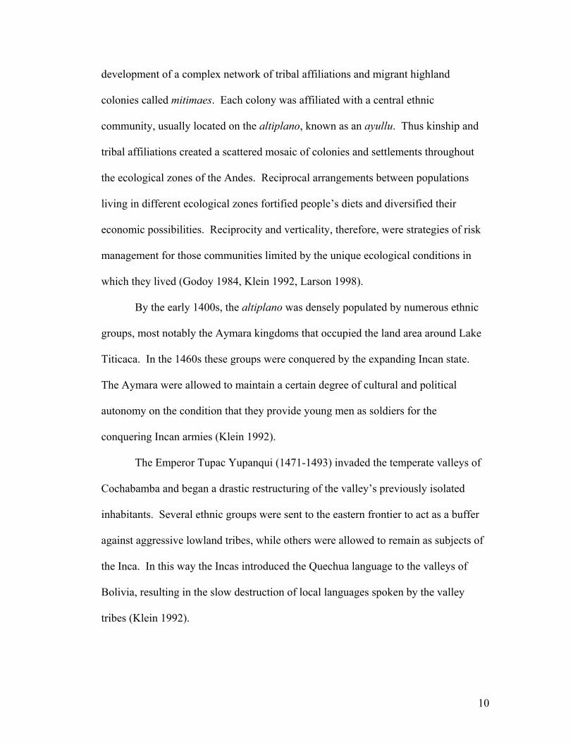
development of a complex network of tribal affiliations and migrant highland

colonies called mitimaes. Each colony was affiliated with a central ethnic

community, usually located on the altiplano, known as an ayullu. Thus kinship and

tribal affiliations created a scattered mosaic of colonies and settlements throughout

the ecological zones of the Andes. Reciprocal arrangements between populations

living in different ecological zones fortified people’s diets and diversified their

economic possibilities. Reciprocity and verticality, therefore, were strategies of risk

management for those communities limited by the unique ecological conditions in

which they lived (Godoy 1984, Klein 1992, Larson 1998).

By the early 1400s, the altiplano was densely populated by numerous ethnic

groups, most notably the Aymara kingdoms that occupied the land area around Lake

Titicaca. In the 1460s these groups were conquered by the expanding Incan state.

The Aymara were allowed to maintain a certain degree of cultural and political

autonomy on the condition that they provide young men as soldiers for the

conquering Incan armies (Klein 1992).

The Emperor Tupac Yupanqui (1471-1493) invaded the temperate valleys of

Cochabamba and began a drastic restructuring of the valley’s previously isolated

inhabitants. Several ethnic groups were sent to the eastern frontier to act as a buffer

against aggressive lowland tribes, while others were allowed to remain as subjects of

the Inca. In this way the Incas introduced the Quechua language to the valleys of

Bolivia, resulting in the slow destruction of local languages spoken by the valley

tribes (Klein 1992).

10

The Emperor Huyana Capac (1471-1527) made further changes in order to

exploit the fertile maize producing valleys of Cochabamba. He resettled highland

tribes to the valleys, creating mitimaes loyal to the Empire. Concurrently, he

developed a system of forced, rotational labor, known in Quechua as the mit’a. Mass

migrations of seasonal laborers came from their highland communities to work in

state owned maize fields. Cochabamba became the maize belt of the Inca Empire,

producing large quantities that were stored in huge stone silos in and around the

Cochabamba valley, later to be shipped throughout the empire to make chicha (maize

beer), or to feed the mass of soldiers in the Incan armies (Larson 1998).

Though less than a century old, the Inca Empire received a shock that resulted

in its ultimate collapse: the arrival of the Spanish. In 1529, the King of Spain granted

Francisco Pizarro the authority and resources necessary to explore and conquer the

regions south of present day Ecuador. Upon Pizarro’s arrival, the empire was

immersed in a civil war of succession that made it vulnerable to the conquistador’s

designs. By the end of the 1530s, the Inca Empire had disintegrated, and in the years

that followed the Spanish destroyed any remaining pockets of resistance (Crivelli

1911).

Once again the Cochabamba valley experienced radical social and political

changes. It retained its role as the maize belt of an empire, but the Spanish system of

labor exploitation and colonialism was markedly different than that of the Incas. In

order to understand the reorganization of valley populations during the early colonial

era, a discussion of Spanish mining efforts in the highlands is essential.

11

In 1545 the Spanish crown, acting through emissaries in South America,

officially established the first mine in the Cerro Rico (rich mountain) of Potosi. So

rich and abundant were the early deposits that veins of pure silver were extracted

from the mountain with little need for processing. Potosi became a boom-town

without precedent. From an initial settlement of 170 Spaniards and 3,000 Indians, by

1610 the city’s population had grown to 160,000 inhabitants. Even by European

standards the city had become a metropolis; Paris had a population of 60,000, London

100,000 (Pacheco et. al. 1997)

A steady output of silver became the primary concern of the early colonial

administration. While introduced diseases decimated the already diffuse Indian

populations, the need for labor in the silver rich mines of Potosi increased

exponentially. In desperate need of a method to exploit Indian labor and extract taxes

from a disperse population, Viceroy Francisco Toledo implemented a series of far

reaching reforms that would forever alter the structure of Andean society. Under

Toledo, the official policy of the colonial regime became “reduction”: the forced

resettlement of the indigenous ayullus into permanent, fixed communities. Though

this was a process that took centuries, Toledo laid the foundation for the destruction

of the dispersed colonies that occurred within the different ecological tiers of the

Andean landscape. In this way the colonial authorities were more easily able to

census and tax the reduced communities (Klein 1992, Larson 1998).

Reduction also solved the problem of a securing a steady supply of labor for

the resource hungry mines of Potosi. The cost of building and maintaining a working

mineshaft was equivalent to the cost of building a cathedral. The Spanish tried a

12

number of tactics to solve the problem of labor shortage, from slavery to wage labor.

The final and most successful of these was the introduction of the mit’a, a Quechua

term used to describe the system of rotational labor used by the Incas in the maize

producing valleys of Cochabamba. Under the Spanish system, one-seventh of the

male population in each community was required to work one year in the mines; each

individual would serve once every six years. Suddenly, the Spanish miners had an

annual labor force of 13,500 men. These men became known as mitayos, obviously

derived from the word mit’a. The Spanish mine owners paid the mitayos a small

wage, which was not even enough for subsistence. The mitayos were required to

provide their own food, coca, and the cost of transportation. The work in the mines

was extremely dangerous, and thousands of men died each year in accidents and from

mining related illness (Klein 1992).

The introduction of the mit’a caused huge demographic shifts in the valley

populations. Suddenly there arose a tension between the Spanish haciendas and the

reducciones, or the nucleated villages created by Toledo’s policy. The new social

order created three distinct groups within the indigenous population: originarios,

forasteros, and yanaconas. The originarios were those who maintained their ties

with their original kin group and were still members of an ayullu. In many instances,

many different ethnic groups became associated with a single reduccion, but all were

lumped into the category of originario in that particular community. They retained

their rights as a member, most notably their rights as land owners, but they were also

subject to taxation and forced labor in the mines. Forasteros were different from the

originarios because they were not original members of the community and they

13

maintained no claim to land in the communities where they lived. They were often

migrant workers, moving from one village to the next, and sometimes became

members of a Spanish hacienda to avoid recruitment for the mit’a. Those who did so

might become members of the yanacona class. These were agricultural laborers who

were subordinate to a Spanish landlord on hacienda lands. The yanaconas were

generally exempt from serving in the mit’a. Because of this highly mobile society,

the colonial administration had to balance the demand for a steady labor force in both

agriculture and mining (Klein 1992, Larson 1998).

Colonial society in Bolivia was a mosaic of free Indian communities and

Spanish haciendas, all tied together by a market economy with its central axis in the

city of Potosi. It was a society dominated by Spanish landholders, bureaucrats, and

mine owners. The entire economy was dependent on the labor of the great mass of

Indian peasants that worked the land and the mines. The economy of Upper Peru was

subject to cycles of boom and bust as mineral production declined and increased

through the years.

In the early 19th century, most of South and Central America was embroiled in

a bloody civil war for independence from the Spanish crown. Simon Bolivar led his

army of liberation against loyalist Spanish troops and won independence for five

South American states: Bolivia, Peru, Ecuador, Colombia, and Venezuela. The

revolution consolidated the power of upper classes in these countries, but did little to

empower the indigenous population of Bolivia. Indigenous members of the new

Bolivian republic were by and large illiterate, and therefore denied the right to vote.

The electoral base was composed of the 30,000 to 40,000 elites that continued to

14

dominate Bolivian politics. The Revolution of 1825 did, however, mark the abolition

of the dreaded mit’a (Klein 1992).

In the 1840’s Chilean workers began to colonize the Bolivian coast to extract

the rich deposits of guano found there. This was the beginning of a 40-year period of

tension and conflicting claims. This ended in 1879, when Bolivia lost the Pacific

War, thus losing claim to its only seaport (Klein 1992). To this day Bolivia and Chile

maintain a tense relationship. Many Bolivians argue that access to the sea is an

economic cure-all that could greatly improve their poverty stricken economy.

In July of 1932, Bolivian President Daniel Salamanca, in response to

escalating tensions in the Chaco area east of the Andes, declared war on neighboring

Paraguay. Thus began the most disastrous military campaign in Bolivian history.

Fighting in the remote Chaco region, the Bolivian army was utterly incapable of

providing its troops with adequate supplies. More people were killed by thirst,

hunger, and disease than by bullets and mortars. Although the loss of their only

seaport in the Pacific War was certainly more damaging to Bolivia’s long-term

prosperity, the Chaco War was longer, bloodier, and more humiliating than any other

conflict in Bolivia’s history (Klein 1992, Knudson 1986).

Long after the last bullet had been fired, the Chaco War continued to send a

wave of disgust and outrage through the Bolivian population. Literate elites began to

question the efficacy of a political system capable of such brutal stupidity. For the

first time, the political ideology of the era expressed its misgivings regarding

Bolivia’s system of land distribution and labor exploitation. The hacienda became

the rhetorical target of these radical intellectuals, who argued that its abolition and the

15

restitution of Indian lands was the only just course of action (Klein 1992, Knudson

1986).

By the early 1950s several political parties were vying for control of the

government. This state of affairs came to a head in 1952, when the Nationalist

Revolutionary Movement (MNR), angered because the military refused to let it take

power after winning the national elections, distributed arms to the civilian population.

In April of 1952 Bolivian civilians, peasants and miners overcame the force of the

military, and the centuries old system of land distribution began to unravel (Klein

1992).

From late 1952 through 1953 armed peasant militias began a complete take

over of the rural countryside. Landowners were expelled, sometimes killed, and the

lands were seized and redistributed among the local population. With the expulsion

of the hacendados, peasant communities began to form sindicatos, which were

responsible for organizing the population, distributing arms, and redistributing land

(Klein 1992, Lagos 1994). In the years that followed indigenous Bolivians

consolidated their land holdings and titles, becoming landowners for the first time

since the Spanish Conquest.

The period after the revolution was one in which the United States began to

play an increasingly important role in Bolivian politics. Food subsidies arrived in

large quantities to mitigate the disruptive effects of the revolution. During the 1970s

the government was in the hands of a military dictatorship that received U.S. support

because of its anti-communist position. In the early 1980s, democracy again took

hold when the military dictatorship relinquished power (Klein 1992).

16

From 1984 to 1985 Bolivia experienced unprecedented rates of hyperinflation.

Structural adjustments during this period curbed inflation rates, but as the threat of

inflation diminished, observers and administrators became increasingly aware that the

Bolivian economy was in desperate need of alternative export products to fill the

vacuum created by the weakened mining economy (Sachs and Morales 1988).

Coca became an important product to fill that vacuum, with disastrous results.

As colonization of the tropical Chapare area in Cochabamba increased, the export of

illegal cocaine came to the forefront of the political forum. Huge sums of money

entered the country through illegal channels. By the late 1980s and early 1990s, the

United States was deeply entrenched as the primary provider of aid dollars to

eradicate illegal coca production in the Chapare and elsewhere (Klein 1992).

Unfortunately, a legal, highly valued product, or better still a suite of such products,

has yet to manifest itself, and the Bolivian economy remains stagnant in the face of

increasing civil unrest and a general feeling of dissatisfaction.

17

CHAPTER IV: STUDY AREA BACKGROUND

GEOGRAPHY

The Tipajara watershed is a tropical mesothermic valley located in the

Province of Mizque. Mizque is located between the following parallels and

meridians:

17 degrees 45 minutes and 18 degrees 30 minutes Southern Latitude 66 degrees 15 minutes and 66 degrees 45 minutes Western Longitude

The watershed delineation presented in Figure 4.1 shows that the Tipajara River

drains into the Mizque River. At its confluence with the Mizque River, the Tipajara

River discharges minimal quantities of water per year (Figure 4.2).

Figure 4.2: Discharge of water, Tipajara river

00.20.40.6

0.81

1.21.4

Jan Feb Mar Apr May June July Aug Sept Oct Nov Dec

Month

m3/

sec

Source: PDAR 1991

18

19

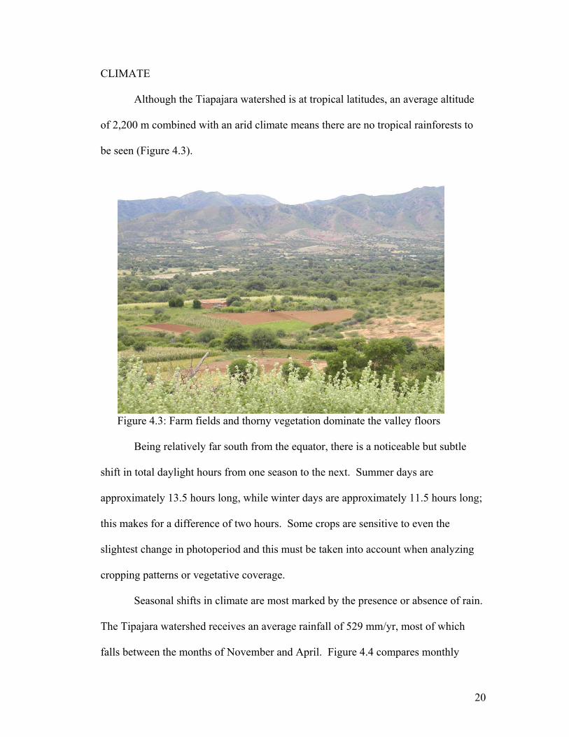
CLIMATE

Although the Tiapajara watershed is at tropical latitudes, an average altitude

of 2,200 m combined with an arid climate means there are no tropical rainforests to

be seen (Figure 4.3).

Figure 4.3: Farm fields and thorny vegetation dominate the valley floors

Being relatively far south from the equator, there is a noticeable but subtle

shift in total daylight hours from one season to the next. Summer days are

approximately 13.5 hours long, while winter days are approximately 11.5 hours long;

this makes for a difference of two hours. Some crops are sensitive to even the

slightest change in photoperiod and this must be taken into account when analyzing

cropping patterns or vegetative coverage.

Seasonal shifts in climate are most marked by the presence or absence of rain.

The Tipajara watershed receives an average rainfall of 529 mm/yr, most of which

falls between the months of November and April. Figure 4.4 compares monthly

20

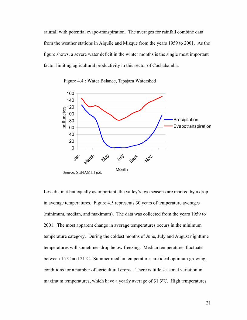
rainfall with potential evapo-transpiration. The averages for rainfall combine data

from the weather stations in Aiquile and Mizque from the years 1959 to 2001. As the

figure shows, a severe water deficit in the winter months is the single most important

factor limiting agricultural productivity in this sector of Cochabamba.

Figure 4.4 : Water Balance, Tipajara Watershed

020406080

100120140160

Jan

March

May July

Sept.

Nov.

Month

mill

imet

ers

PrecipitationEvapotranspiration

Source: SENAMHI n.d.

Less distinct but equally as important, the valley’s two seasons are marked by a drop

in average temperatures. Figure 4.5 represents 30 years of temperature averages

(minimum, median, and maximum). The data was collected from the years 1959 to

2001. The most apparent change in average temperatures occurs in the minimum

temperature category. During the coldest months of June, July and August nighttime

temperatures will sometimes drop below freezing. Median temperatures fluctuate

between 15ºC and 21ºC. Summer median temperatures are ideal optimum growing

conditions for a number of agricultural crops. There is little seasonal variation in

maximum temperatures, which have a yearly average of 31.3ºC. High temperatures

21

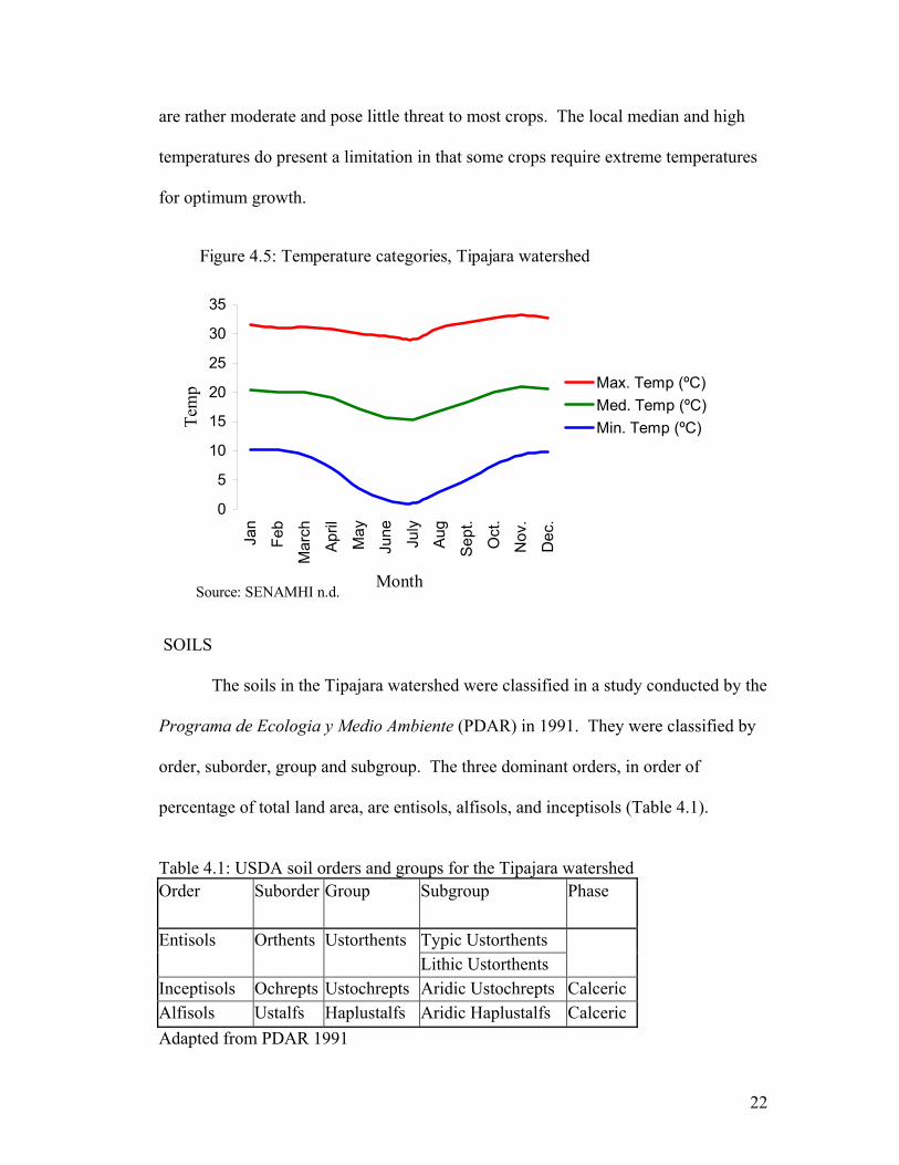
are rather moderate and pose little threat to most crops. The local median and high

temperatures do present a limitation in that some crops require extreme temperatures

for optimum growth.

Figure 4.5: Temperature categories, Tipajara watershed

0

5

10

15

20

25

30

35

Jan

Feb

Mar

ch

April

May

June July

Aug

Sept

.

Oct

.

Nov

.

Dec

.

Month

Tem

p Max. Temp (ºC)Med. Temp (ºC)Min. Temp (ºC)

Source: SENAMHI n.d.

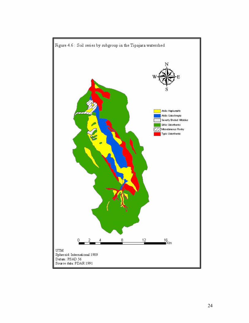
SOILS

The soils in the Tipajara watershed were classified in a study conducted by the

Programa de Ecologia y Medio Ambiente (PDAR) in 1991. They were classified by

order, suborder, group and subgroup. The three dominant orders, in order of

percentage of total land area, are entisols, alfisols, and inceptisols (Table 4.1).

Table 4.1: USDA soil orders and groups for the Tipajara watershed Order Suborder Group Subgroup Phase

Typic Ustorthents Entisols Orthents Ustorthents Lithic Ustorthents

Inceptisols Ochrepts Ustochrepts Aridic Ustochrepts Calceric Alfisols Ustalfs Haplustalfs Aridic Haplustalfs Calceric Adapted from PDAR 1991

22

Table 4.2: Characteristics and distribution of dominant subgroups in the Tipajara watershed

Subgroup of Dominant Soils

Physiographic Features Hectares %

Aridic Haplustalfs* Plains with gentle to moderate slopes. Prairies at the foot of mountains. High terraces.

4,043 16.5

Aridic Ustochrepts* Prairies at the foot of mountains. High terraces. Low terraces

1,992 8.1

Eriales Eroding Hillsides 94 0.4 Mountains with steep slopes. Mountains with moderate slopes.

Lithic Ustorthents

Hills at the foot of mountains.

11,442 46.7

Miscellenous Rocky Escarpment of plains 3,850 15.7 Mountains with moderate slopes.Hills at the foot of mountains.

Typic Ustorthents*

Low terraces

2,746 11.2

River Bed 320 1.4 Adapted from PDAR 1991 *primary soils for onion production

Figure 4.6 shows a map for the different soil subgroups in the Tipajara watershed.

A detailed summary of the physical and chemical characteristics of these soils can be

found in Appendix I.

23

24

FAMILY NUTRITION

Most families primarily consume foods rich in carbohydrates. Rice, maize

and potatoes are the staples of the vast majority. These are often eaten in soups,

sometimes mixed with different vegetables grown locally. Fresh meat is uncommon,

perhaps consumed on average once a week. Eggs are a primary source of protein,

though dried jerky is a common component of soups. During the months of March,

April, and May, fruit is often picked from trees scattered in the fields. Families tend

to consume carbohydrates at the expense of other important foods. Most notably

there is a glaring lack of protein and dairy in the local diet, but fruit and vegetables

are also consumed sporadically. Figure 4.7 illustrates the generally poor level of

nutrition experienced by most children under 5 in the community of Tipa Tipa. Free

check-ups at the local health center are only available for children under 5 years and

pregnant mothers; this explains why the data only cover this age group.

Figure 4.7 : Nutritional state of children under 5 years, Tipa Tipa Based on local classification

2%

49%

35%

11%

3%

SuperiorNormalSlightModerateSevere

Source: Distrito X de Salud Mizque (SNISII)

25

It is quite possible that levels of malnutrition are much higher in other communities

that are more water limited, as these communities are unable to grow vegetables or

fruit trees.

HISTORY

The Pre-Incaic valleys of Mizque were most probably occupied by

agriculturalist tribes that also relied on hunting and gathering as a means of

subsistence. Various rock paintings have been found in the area depicting different

zoomorphic and anthropomorphic figures (Figure 4.8).

Figure 4.8: Pre-Columbian zoomorphic figures near the town of Mizque Photo courtesy Brad David Kennedy

A common theme in many of these paintings is hunting, suggesting that wildlife and

forests provided important products to early human settlements in the area.

26

Around 1480 the Inca sent a mitimae colony of Aymara speaking Chuy people

to settle the Mizque valley. The group was sent to defend the eastern frontier from

aggressive Guarani speaking tribes, known as the Chiriguano (Gade 1999). Many

fortifications were built along the eastern frontier to defend the empire from

Chiriguano incursions; the most famous of which can be seen at Incallajta several

kilometers from the town of Pocona (Swaney 2001).

Forty years after the Conquest, Viceroy Francisco Toledo founded the

reducción of San Sebastian de los Chuyes, known by the local inhabitants as Mizque,

with the expressed intent of creating a nucleated village that would prevent further

Chiriguano incursions. Spaniards found the location attractive and migrated there for

several reasons. Flat, fertile soils, a warm climate and abundant water from the

Mizque River created favorable conditions for agriculture. The climate permitted a

diet of wheat bread and wine from fermented grapes, reminiscent of the

Mediterranean foods that the Spanish preferred. Forest resources and fish were also

in great supply (Gade 1999).

The location was also economically advantageous. The mining metropolis of

Potosi, surrounded as it was by poor soils and cold, dry conditions, relied primarily

on imports from the altiplano, valleys, and yungas for its supply of agricultural

products. Mizque was well situated between Cochabamba, Sucre, and Potosi, which

made it a primary destination along this important trading route and an important

producer in its own right (Gade 1999). Figure 4.9 shows a colonial bridge on the road

between Cochabamba and Mizque.

27

Figure 4.9: El Puente de los Libertadores, called so because Simon Bolivar passed across this bridge on his travels to the cities of Sucre and Potosi Photo courtesy Brad David Kennedy

By the 18th century Mizque had a population of 22,000 and was well

established as one of the most important towns in Upper Peru. The Catholic Church

had a strong presence in Mizque. With several religious orders and a cathedral, the

pleasant town of Mizque acted as the defacto seat of the diocese for several bishops

that preferred it to the much hotter climate of Santa Cruz de la Sierra (Figure 4.10).

Mizque also had a hospital, only one of seven in all of Upper Peru (Gade 1999).

28

Figure 4.10: The newly restored Cathedral in Mizque Photo courtesy Brad David Kennedy

The hacienda was the primary producer of agricultural goods. The haciendas

of Mizque relied heavily on yanacona laborers, who were often descendants of the

highland Indians that fled their communities in an attempt to escape from the mit’a.

Wine producing haciendas relied primarily on African slaves to perform most of the

tasks on the vineyard. Some haciendas were so large that they had access to both

highland areas (>3000 m) and valley lands. The highest areas were used to graze

cattle, sheep, and horses, while lower, unirrigated slopes were used to cultivate wheat,

maize, quinoa, barley, pulses, and potatoes. Irrigated lands in the valley bottoms

were used to produce native crops, like sweet potato, ahipa, maize, and yacon , and

29

introduced crops like sugar cane, cotton, tobacco, and grapes. Many different fruits

also became commonly cultivated in irrigated parcels: avocado, cherimoya, pacay,

banana, orange, fig, apple, quince, and peach (Gade 1999).

Mizque’s economy was linked to the greater economy of Upper Peru through

its abundant natural resources. Enormous quantities of wine were exported to the

insatiable markets of Potosi. Declines in the mining economy in the early 18th

century decreased the demand for wine, and grapes were superceded in importance by

local varieties of chili pepper. Mizque was also a supplier of honey, wheat, horses,

wax, and cotton. Timber was also sent to Potosi for use in making mining equipment.

Cedro (Cedrela spp.), a local forest tree, was exported as a prime cabinetry wood

(Gade 1999).

This era of prosperity did not last. In the early 18th century Mizque began a

long and steady decline. In 1710 the town of Mizque was ravaged by an epidemic of

fevers that eliminated half of its population. By 1771 the Chuy Indians, descendents

of the original mitimae colony, had been almost completely wiped out by malaria.

All segments of the population experienced this decline: from the Spanish vecinos to

the indigenous originarios, forasteros, and yanaconas. The decline in the native

population resulted in the subsequent collapse of the hacienda economy, as labor

became scarce and existing laborers were often too sick to work at full capacity. The

only group that seemed to flourish were the people of African ancestry, who made up

30 percent of the population in the valleys of Mizque by the year 1787 (Gade 1999).

Malaria was the causal agent responsible for Mizque’s demographic collapse.

At this time, people were not well equipped to deal with malaria and its horrible

30

consequences. They were unaware that the mosquito was the primary vector of the

disease; they were equally oblivious to the fact that Mizque, with its warm climate

and its floodplains and stagnant puddles, was the perfect breeding ground for this

fatal pest. The result was disastrous (Gade 1999).

Unable to avoid infection by remaining in the Mizque valley, most people

developed different strategies to minimize the risk of contracting malaria. Some

Spanish landowners fled to the upland areas of their haciendas, while others

abandoned the area and moved to the nearby city of Cochabamba. Traveling

merchants learned to bring their llama trains through Mizque during the dry season,

when the risk of malaria infection was relatively low. Resistance to the disease

played an important part in determining the composition of the population. Africans

seemed to have the most genetic resistance to the disease, most likely because of

exposure in their native continent, followed by the Spanish, who were also exposed to

malaria on the Iberian Peninsula. The indigenous population seemed to suffer the

most, and this partly explains why most mizqueños are now mestizos (Gade 1999).

Interestingly, the African population has totally disappeared from present-day

Mizque.

The early 20th century showed no improvement in the centuries long malaria

crisis that gripped the region. Between 1908 and 1940, 40 percent of the deaths that

occurred in the area were attributed to malaria. From 1922 to 1929, 70 percent of all

deaths were attributed to the disease. Yet advances in science and medicine were to

change this. Modern science had identified the mosquito as the vector of malaria, and

in the three years between 1929 and 1932, a massive effort was made to eliminate

31

standing water from Mizque. Homes were fumigated and whitewashed, and quinine

was made available to those individuals that tested positive for malaria. A nation

wide epidemic in the early 1940s drew further attention to the problem, and Mizque

was fumigated with DDT while new synthetic drugs were distributed to the unhealthy

population. These tactics finally yielded a measurable result: by 1951 not a single

person in the town of Mizque tested positive for malaria (Gade 1999).

The valleys of Mizque underwent major changes in the years that followed the

centuries long battle with malaria. Coincidentally, malaria was brought under control

at the same time that the Agrarian Reform was getting underway. The haciendas

were destroyed and their lands were divided amongst the landless sharecroppers.

Between 1950 and 1976 Mizque experienced a 32 percent increase in population;

many of the newcomers came from the Cochabamba valley in search of unoccupied

agricultural land. The eradication of malaria also caused a drastic reduction in infant

mortality. By the 1980s, 50 percent of the population was under 20 years old.

Irrigation expanded to cover 70 percent of the valley floors, and the years between

1955 and 1967 saw a doubling in agricultural productivity. Improved infrastructure,

such as roads, electricity, water, and sewage also improved living conditions and once

again connected Mizque with the broader Bolivian economy. In short, the eradication

of malaria spurred the development of the Mizque valleys (Gade 1999)

32

CHAPTER V: METHODS AND DATA

PROJECT BACKGROUND

The data collection for this study was undertaken as part of an integrated farm

systems management project that I executed in collaboration with the community of

Tipa Tipa and the Bolivian non-governmental organization (NGO) PLAN. After a

year and a half of fieldwork with my community counterpart, we both believed that

alternative forms of production were necessary if local farmers were to have any hope

of achieving sustainable production and a steady income over the long term. My

assumption that onion production was unstable, based on field observations, led me to

design and present a written grant proposal to PLAN. In the process of writing the

proposal, it was agreed that the project budget would include money for the hire of

two field technicians. Their job was to work in collaboration with the Peace Corps

volunteer to design and implement a cost-benefit analysis and a general farm systems

analysis for the Tipajara watershed. The data would then be used as a basis for

understanding the current state of agricultural production and to identify constraints

to future increases in productivity. After completing the data collection, I presented

PLAN with a general summary of the cost-benefit data and the demographic data

collected for the Tipajara watershed. PLAN will use the data to design future projects

in agriculture, forestry, health, and family nutrition. In addition, it was agreed that I

would use the data to prepare my thesis.

33

STUDY METHODOLOGY

Though much of the data presented in this thesis is based on a quantitative

model that I developed through survey questionnaires, there is a great deal of

information included that was gathered through participant observation. Essentially,

a participant observer is a researcher who is completely immersed in the community

and culture being studied. Though Peace Corps and participant observation are two

distinct phenomena, they are certainly complementary, as Peace Corps provides the

researcher with the perfect opportunity to participate in all aspects of community life.

All of the data presented in this thesis, whether quantitative or qualitative, rests on the

firm foundation that I laid in the early months of my Peace Corps service as a

participant observer. Participant observation requires knowledge of the local

language, an awareness of the cultural forces at work in people’s daily lives, and the

trust of local people that inevitably builds as the observer becomes a fixture in the

community, which allows people to go about their activities in a normal fashion

(Bernard 2002, Nichols 2000).

I used key informants quite extensively as a means of understanding changes

in the farm system over time (Bernard 2002). Key informants provided me with

important information on the following topics: local history, changing cropping

patterns, family lineages, and incidence of disease through time.

Many researchers with experience in the developing world have emphasized

the importance of pilot testing as a means of avoiding irreparable errors in the main

data collection phase of a research survey (Devereux and Hoddinott 1993). Nichols

(2000) defines a pilot survey, or a pre-test, as “a small survey, in advance of the main

34

fieldwork, to test the form, sampling procedures and fieldwork management

procedures” of the study being conducted. The pre-test for this study was done in

September of 2001, when fellow PCV Kitri Falxa and I designed the survey forms

and interviewed 25 farmers in Tipa Tipa to calculate the cost of production and net

income for the onion production cycle of 2001. This experience allowed me to

design, and later refine, the survey forms that were used in the main survey, to

understand the potential pitfalls certain questions may have, and to develop a

statistical sampling methodology.

I was also given the opportunity to further refine the survey form when, in

August of 2002, I attended a workshop in the city of Cochabamba with several

farmers from Tipa Tipa and the two field technicians who would do the interviews for

the study. In this workshop, as a group activity, we calculated the real costs of

production with the four local farmers. During the activity, the farmers were able to

point out several hidden production costs that I had overlooked in the initial survey

design.

I had to confront several important considerations and limitations when I was

designing the study. To make the population size manageable, and in consideration

of the mountainous geography of the Mizque Province, we agreed to limit the study

to the geographic area of the Tipajara watershed. Considering the profound

ecological differences due to extreme changes in elevation over relatively short

distances, watersheds are a logical unit of measure for any natural resource

management program in the rural valleys of Bolivia.

35

Since PLAN was financing the data collection process, they required that the

data be collected only from communities in which PLAN was currently working.

Due to the nature of PLAN’s fiscal structure, they are very strict about working in

communities that have gone through the lengthy process of formally affiliating

themselves with the NGO. Based on these two criteria, we were able to make a

preliminary list of the communities to be included in the study. They are:

Loro Mayu Montecillos Rumi Cancha San Pedro Alto San Pedro Bajo Taboada Tipa Jara Grande Tipa Jara Chico

Tipa Tipa

Rumi Cancha, San Pedro Alto, and Tipajara Chico were eliminated from the list

because these three communities have less irrigation water and only cultivate onions

on a small, non-commercial scale. It should be noted here that Khuru Mayu is the

only significant onion producing community in the Tipajara watershed that is not on

the list. It is therefore unlikely that this sampling methodology introduced any

significant bias into the study. It was not possible to include Khuru Mayu in the

study because they had no affiliation with PLAN.

After deciding which communities were to be included in the study, I required

a sampling frame to determine the number of onion farmers in each community

(Bernard 2002). Every community in this sector of Bolivia is organized into

sindicatos, which are the equivalent of village governments. Though not every

community member is affiliated with the sindicato, I estimate that approximately

36

95% of households are affiliated and listed in the registry. Unmarried males with no

children are less likely to be affiliated than any other demographic group. The hired

field technicians visited each village during a community meeting to explain the

nature of the study and to ask permission to conduct the study. Once the community

granted permission to conduct the study, the field technicians were allowed access to

the sindicato registry, which has all the names of affiliated household heads. At this

point, the community of Tipajara Grande indicated that they did not want to

participate in the study, and this community was subsequently eliminated from the

list.

Once a full list of all affiliated members was obtained for each community, I

divided each household into two categories: onion producers and non-onion

producers. This was done through verbal verification with a member from each

community. To summarize, the population from which I took the sample was

determined by the following characteristics: all onion-producing households in the

Tipajara watershed affiliated with the sindicato in communities associated with

PLAN. After I acquired the sampling frame, I used the following equation to

determine the sample size:

x2NP (1-P)

C2 (N-1) + x2 P(1-P) Where x2 is the chi square value for 1 degree of freedom at a desired probability level.

N is the population of onion farmers in the five communities and C is the confidence

interval, which I set at 5%. P is the population parameter of a variable, which in this

case I set to 0.5 (Bernard 2002). Once the total sample size was calculated, I used the

37

proportional allocation method to determine the number of households to be included

from each community. In this procedure the proportion of the sample that was

selected from each community was equal to the proportion of all households within

that community (Freese 1984). The calculation had the following results:

Table 5.1: Sample size by community

Community #* Community Name # of onion producers # in sample

1 Loro Mayu 20 10 2 Tipa Tipa 100 55 3 Montecillos 69 32 4 Taboada 73 40 5 San Pedro Bajo 60 32

Total 322 169 *The numbers assigned to each community will be used instead of names

Working through the calculation, one quickly realizes that the total number in the

sample at a 5% confidence interval should be 175. These 6 households were

eliminated from the survey at the very end because they had proven extremely

difficult to find, and the field technicians were tired of the enormous amounts of

footwork required to find each farmer. The sampling method was a simple random

sample. I assigned a number to each household; I then used a random number

generator in MS Excel to select each household to be interviewed (Bernard 2002).

38

39

Figure 5.1: Study communities by number

The two field workers responsible for the data collection, Toribio Maygua and

Mario Huanca, were undergraduate students hired from the University of San Xavier

de Chuquisaca. Hiring field workers to conduct interviews provided several

advantages. The first and most obvious was the increase in manpower needed to

complete the interviews in a reasonable amount of time. Técnicos, as described by

Boa et. al. (2001), also provide other advantages. Their ability to communicate

effectively with both scientists and local farmers is an important bridge between the

two cultures, and in this particular case their mastery of both Quechua and Spanish

proved an invaluable skill when dealing with semi-literate, often times monolingual,

Quechua families.

Bernard (2002) explains that using multiple interviewers has several distinct

disadvantages, as well. For example, each interviewer may introduce bias into the

study. This is especially the case when the survey involves complex or embarrassing

social issues and/or open-ended questions. I minimized the potential for interviewer

bias in a number of ways. First, the questionnaire used only forced choice questions,

which generally avoided sensitive or embarrassing potential responses. Furthermore,

I trained the interviewers in tandem to ensure that their method of asking the

questions was both uniform and unambiguous. I was able to anticipate potential

misunderstandings because of the survey pre-test performed the year before. The

interviewers were each required to do several mock interviews to ensure that they

asked the questions in a uniform and consistent manner (Nichols 2000). This practice

was followed by several trips to the field where I monitored the field workers to

verify that they were asking the questions in the appropriate manner. Once the field

40

technicians reached a satisfactory level of skill in conducting interviews, they were

required to observe one another at regular intervals to guarantee that their method of

interviewing remained consistent throughout the interview process. All participants

were informed in their native language of Quechua that their participation was

voluntary, and at any time they could choose to terminate the interview. This

research was conducted following Human Subject Research guidelines and was

approved by the Michigan Technological University Institutional Review Board.

It must be noted that we were forced to change the names in the random list a

number of times. However, these changes were only made when absolutely

necessary. Some families on the list had moved within the past year. Some families

refused to participate, and other families did not cultivate any onions for the 2002

cropping cycle. Whenever this happened, the family was eliminated from the list and

another family was randomly selected from the original sampling frame. It took

approximately 4 months to complete all 169 surveys

During the data entry process, I tried to filter out biased or illogical responses

within the survey data. In any instance where the information on the data sheets

looked unusual (e.g. extremely high or low numbers) or in some cases was illegible, I

consulted with the field technicians to confirm the information. There were several

instances when I personally consulted with the interviewed farmer just to make sure

his response was correct. In an overwhelming majority of the cases, from my

experience and the experience of the field technicians, the farmers did their best to

provide honest responses to the best of their knowledge.

41

I also had the opportunity to use a geographic information system (GIS) to

generate the maps that are used in this thesis. I used GIS to determine ground cover

from satellite images, to create tenure maps based on aerial photos, and to show

changes in land use, land cover, and infrastructure over time (Burrough and

McDonnell 1998, Chang 2002). The primary GIS packages that I used were ARC

View, ARC Map, ERDAS Imagine, and ILWIS.

UNIVARIATE STATISTICS

This is a brief summary of the data set for the household survey conducted in

the Tipajara watershed in the 2002 cropping season. Table 5.2 summarizes the

physical inputs used for onions production. Table 5.3 summarizes these values in

economic terms, and Table 5.4 summarizes the economic indicators of production.

At the time of the study, USD $1 was equivalent to Bs. 7.45. These are the most

relevant and logical variables for analyzing onion production in the Tipajara

watershed. Differences in community are not shown in these summaries, but will be

addressed using more rigorous statistical tests in the results and discussion chapter.

Table 5.5 shows some of the basic demographic characteristics of the study

population by community. Table 5.6 is a census of the average number of animals for

each family by community. Generally, those families and/or communities with more

animals have less irrigation.

42

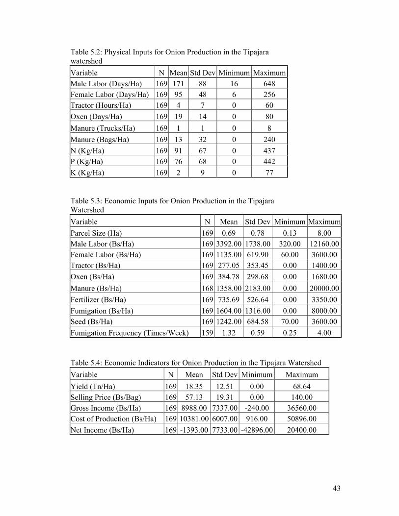
Table 5.2: Physical Inputs for Onion Production in the Tipajara watershed Variable N Mean Std Dev Minimum Maximum Male Labor (Days/Ha) 169 171 88 16 648 Female Labor (Days/Ha) 169 95 48 6 256 Tractor (Hours/Ha) 169 4 7 0 60 Oxen (Days/Ha) 169 19 14 0 80 Manure (Trucks/Ha) 169 1 1 0 8 Manure (Bags/Ha) 169 13 32 0 240 N (Kg/Ha) 169 91 67 0 437 P (Kg/Ha) 169 76 68 0 442 K (Kg/Ha) 169 2 9 0 77

Table 5.3: Economic Inputs for Onion Production in the Tipajara Watershed Variable N Mean Std Dev Minimum MaximumParcel Size (Ha) 169 0.69 0.78 0.13 8.00 Male Labor (Bs/Ha) 169 3392.00 1738.00 320.00 12160.00Female Labor (Bs/Ha) 169 1135.00 619.90 60.00 3600.00Tractor (Bs/Ha) 169 277.05 353.45 0.00 1400.00Oxen (Bs/Ha) 169 384.78 298.68 0.00 1680.00Manure (Bs/Ha) 168 1358.00 2183.00 0.00 20000.00Fertilizer (Bs/Ha) 169 735.69 526.64 0.00 3350.00Fumigation (Bs/Ha) 169 1604.00 1316.00 0.00 8000.00Seed (Bs/Ha) 169 1242.00 684.58 70.00 3600.00Fumigation Frequency (Times/Week) 159 1.32 0.59 0.25 4.00

Table 5.4: Economic Indicators for Onion Production in the Tipajara Watershed Variable N Mean Std Dev Minimum Maximum Yield (Tn/Ha) 169 18.35 12.51 0.00 68.64 Selling Price (Bs/Bag) 169 57.13 19.31 0.00 140.00 Gross Income (Bs/Ha) 169 8988.00 7337.00 -240.00 36560.00 Cost of Production (Bs/Ha) 169 10381.00 6007.00 916.00 50896.00 Net Income (Bs/Ha) 169 -1393.00 7733.00 -42896.00 20400.00

43

Table 5.5: Demographic Averages per Household in the Tipajara Watershed Community 1 Community 2 Community 3Community 4Community 5Tipajara WatershedFamily Size (Persons/Household) 8 6 7 6 6 6Total Arable Land (Ha/Household) 3.1 2 2.9 1.8 1.9 2.2 Catholic (%) 100 68 82 92 88 81Evangelist (%) 0 32 15 8 13 17Father's Age 49 40 44 43 41 42Father's Education (Grade Level) 4 5 3 5 5 5Mother's Age 47 37 44 43 39 41Mother's Education (Grade Level) 3 4 3 4 3 3

Table 5.6: Mean Number of Animals per Household in the Tipajara Watershed Community 1 Community 2Community 3Community 4Community 5Tipajara WatershedChickens 8 2 6 4 5 4Cows 8 3 4 2 3 3Donkeys 2 0 0 0 0 0Goats 26 2 10 6 6 7Pigs 1 1 2 1 2 1Sheep 15 5 11 1 3 6Total 59 13 34 14 19 21

44

MULTIVARIATE STATISTICAL METHODS

Once the data had been entered and properly summarized, I used Statistical

Analysis Software (SAS) to perform a number of statistical tests. First, I analyzed the

data using a Pearson test for correlation, which allowed me to decide what further

statistical tests were required. The Pearson test showed that there were many

relationships between the variables for onion production. Demographic variables

revealed fewer relationships; those relationships that did exist had higher P-values

and were therefore weaker. The Pearson test demonstrated that the data were

excellent for creating a multivariate regression model (Hill, Griffiths, and Judge

1997). I then used SAS multivariate regression technique to generate two

multivariate regression models: one for yield and another for net income.

I also used an ANOVA test of significance to test differences across these

categorical distinctions: community, parcel size, and winners/losers. An ANOVA

test of significance only shows that a difference exists. When more than two

categories exist for each variable, the ANOVA does not indicate where the

differences exist between categories. I therefore selected all those tests that were

statistically significant for further analysis. I then used Tukey’s w-procedure, which

allowed me to ascertain which differences within each category were significant and

which were not (Steel and Torrie 1960).

45

CHAPTER VI: RESULTS AND DISCUSSION FOR TENURE AND LAND USE

Changes in land use and land tenure in the years that followed the eradication

of malaria drastically changed the structure of society and the nature of agricultural

production in the Tipajara watershed. Linked as it is to the greater towns of Mizque

to the North and Aiquile to the South, the Tipajara watershed experienced the same

changes that the Mizque valley did in the years following 1952. During my time as a

Peace Corps volunteer, I took a particular interest in this transformation and how it

shaped changes in agriculture. This chapter documents the intensification process

during this period, and it provides important information for understanding the reality

and the consequences of a cash crop monoculture for the farmers in the Tipajara

watershed.

PRE-REFORM SOCIETY

Throughout its history, the Tipajara watershed has been an agricultural valley

that links the two larger towns of Aiquile to the South and Mizque to the North.

Evidence of pre-Colombian peoples is not scarce: from stone fortifications on

mountaintops to shards of pottery in farm fields to pre-Incan rock paintings depicting

hunting scenes. The people that live in the area have no memory of these distinct

cultures, nor are their histories preserved through oral tradition.

Ethnographer Georges Rouma (1933) gives an account of the culture of the

Quechua Indians living in the hacienda of Novillero in the era before the Agrarian

Reform. Novillero is approximately 30 km. from the Tipajara watershed. Some of

the customs and traditions he describes have long since disappeared, others remain in

46

the more isolated communities, and others are still a part of the daily life of the

Quechua speaking campesinos in the area.

Rouma describes a culture that was still very much self-sufficient in providing

most of the needs for the daily household. Clothing was generally produced from

sheep’s wool, which was produced on-farm. Women were responsible for shearing

the sheep and turning the wool into yarn, which was then used to weave ponchos,

pants, sweaters, and even hats. Men were responsible for building the home, the

base made of stones, the walls of adobe bricks, and the roof from mud and sticks.

The household also produced a number of useful domestic products: ceramics,

knives, picks, and sandals. A variety of plants and trees were used for wood,

medicine, and food (Rouma 1933).

The farm system was based primarily on the production of cereals. Maize was

a staple crop produced and consumed on-site. Surplus might be sold to the city, but

the majority of the surplus was stored in a silo made from the hard branches of the

chacatea shrub (Dondonea viscosa) (Figure 6.1).

47

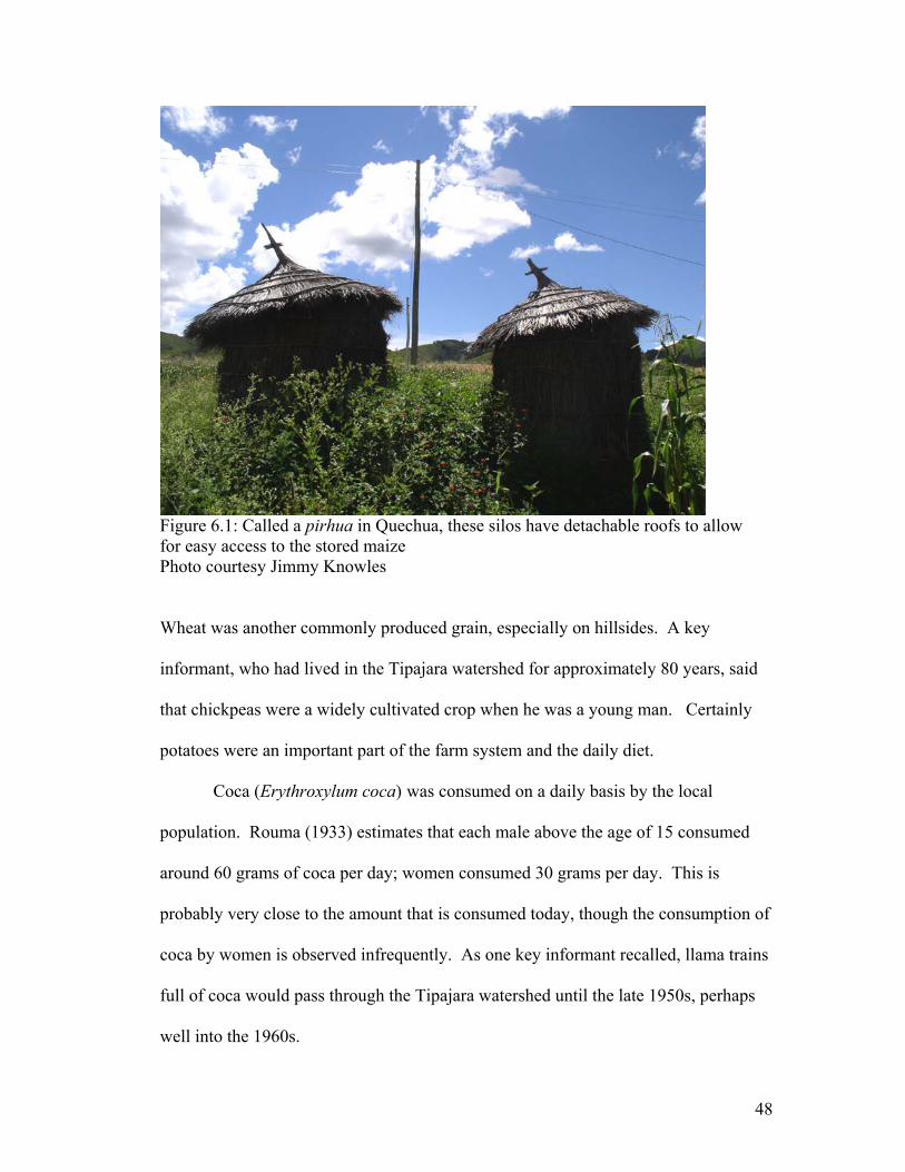
Figure 6.1: Called a pirhua in Quechua, these silos have detachable roofs to allow for easy access to the stored maize Photo courtesy Jimmy Knowles Wheat was another commonly produced grain, especially on hillsides. A key

informant, who had lived in the Tipajara watershed for approximately 80 years, said

that chickpeas were a widely cultivated crop when he was a young man. Certainly

potatoes were an important part of the farm system and the daily diet.

Coca (Erythroxylum coca) was consumed on a daily basis by the local

population. Rouma (1933) estimates that each male above the age of 15 consumed

around 60 grams of coca per day; women consumed 30 grams per day. This is

probably very close to the amount that is consumed today, though the consumption of

coca by women is observed infrequently. As one key informant recalled, llama trains

full of coca would pass through the Tipajara watershed until the late 1950s, perhaps

well into the 1960s.

48

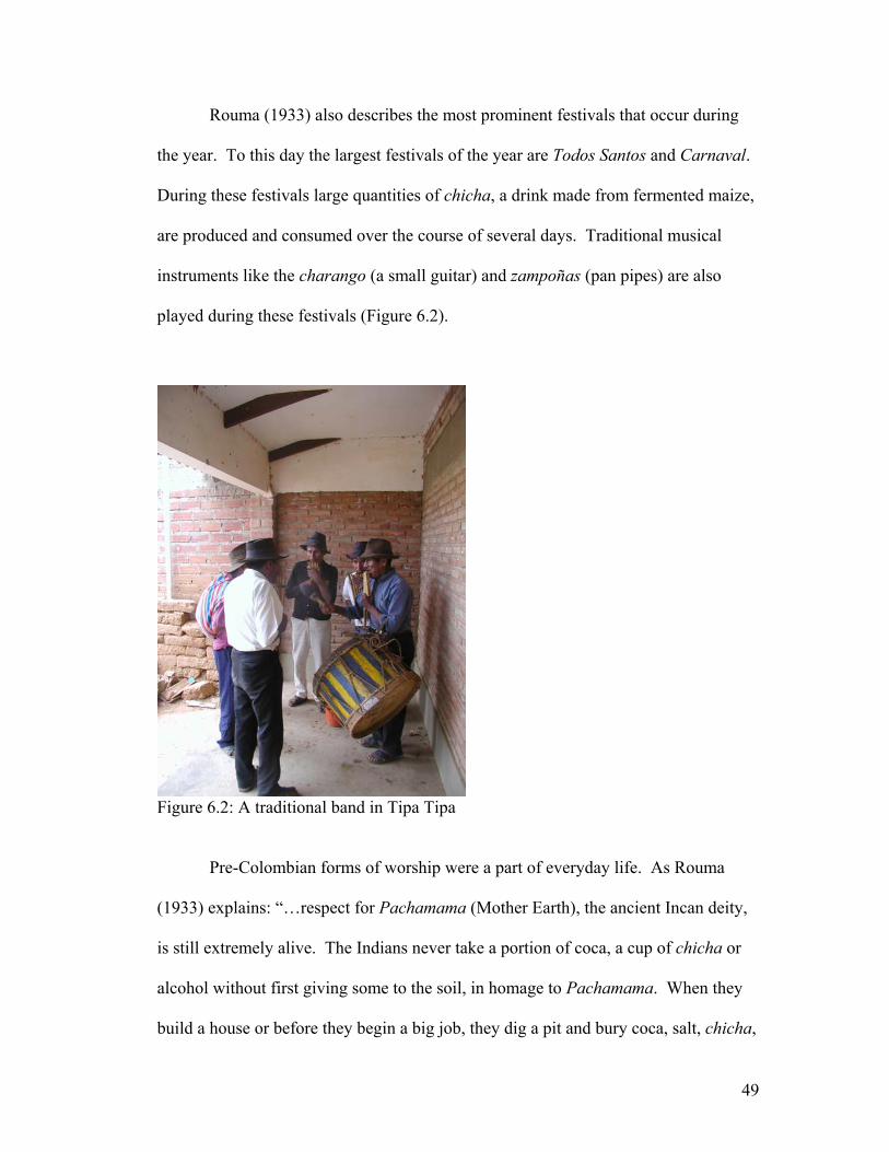
Rouma (1933) also describes the most prominent festivals that occur during

the year. To this day the largest festivals of the year are Todos Santos and Carnaval.

During these festivals large quantities of chicha, a drink made from fermented maize,

are produced and consumed over the course of several days. Traditional musical

instruments like the charango (a small guitar) and zampoñas (pan pipes) are also

played during these festivals (Figure 6.2).

Figure 6.2: A traditional band in Tipa Tipa

Pre-Colombian forms of worship were a part of everyday life. As Rouma

(1933) explains: “…respect for Pachamama (Mother Earth), the ancient Incan deity,

is still extremely alive. The Indians never take a portion of coca, a cup of chicha or

alcohol without first giving some to the soil, in homage to Pachamama. When they

build a house or before they begin a big job, they dig a pit and bury coca, salt, chicha,

49

pepper. These are offerings to Pachamama.” Though the intensity of these customs

has been dulled somewhat by modernization, families still make these offerings to

Pachamama.

One key informant was particularly useful in providing a great deal of

information about Tipa Tipa in the era prior to and during the Agrarian Reform.

From here forward, I will refer to him as Don Pedro. Don Pedro was born in 1941.

He lived through the Reform as a young boy, and was always eager to explain times

past. I would visit him often, and his stories became very much a part of my field

notes as I tried to reconstruct the local history. He was the son of a sharecropper who

lived on the hacienda of Josefina Betancur and her son Don Alberto Torrico. Though

not required to work and live on the hacienda, most sharecroppers did so because all

of the best lands were owned by the patrones (Klein 1992). Josefina and Alberto

were the patrones of the area known as Tipa Tipa, called so for the presence of two

oversized Tipa trees (Tipuana tipu) located within the boundaries of the community.

Don Pedro’s parents were known as colonos, the pre-reform word for

sharecroppers; in colonial times sharecroppers were labeled yanaconas. Don Pedro’s

parents were illiterate and were obligated to fulfill several services to the patron.

First, they had to pay a rent fee to the patron for use of the land, this was known as

the jullk’a in Quechua. Added to the heavy workload of subsistence agriculture, the

colonos had to maintain the personal fields and flocks of the patron as well. Each

family was also required to give 10 percent of the maize harvest and 10 animals

annually. This system was known as the pongueaje. The patrones lived in the city

and went to the countryside to collect payments and for vacations.

50

In 1947, Pedro attended school for the first time. It was the patrones

themselves that helped with the establishment of the school for young male children.

The school moved from house to house and never met with much success. Despite

these token attempts at education, the society was very repressive. Community

meetings were forbidden. Games were also not permitted. People were unaware that

the game of soccer existed. The farmers spoke only Quechua. Very few people

spoke or understood Spanish beyond the basics.

THE AGRARIAN REFORM OF 1952

In the year 1952, all of this was about to change. “The land is for those who

work it,” was the call to arms of the then disenfranchised colonos. In Tipa Tipa,

clandestine meetings were held at night or in out of the way places. Then, one day, as

Pedro described it:

We went to the hills behind our house. In those days we used to plant maize in the hills too; and we were out there harvesting our maize when we heard the sound of a pututu blowing just down below, near the river. Then we heard another one from further away, and another, till the whole valley was full of the sound of the blowing pututu. It was the reforma agrarian. It had come.

The pututu is a Quechua word for a cow’s horn that is blown into to inform

the people that a meeting is being called. In this case, the many sounds of the pututu

were a call to arms. Pedro, then 11 years old, and his older brother rushed to see what

was happening. At the meeting he saw over 1,000 colonos that had come from

nearby communities. Word had finally reached the area that the agrarian reform was

a reality, and the people began to organize themselves to remove the patron and

51

redistribute the land. In Tipa Tipa, the patron escaped in the night, and no blood was

spilled.

With the disappearance of the patrones, community self-government began to

flourish, and a tradition of democratic self-rule established itself in Bolivia’s rural

sectors. By 1954, Tipa Tipa formally established itself by forming a sindicato. The

sindicato is a village government responsible for conflict resolution, organizing

community activities, and identifying and implementing community projects. The

sindicato of Tipa Tipa is headed by the dirigente. He is always a man, and he is

elected once a year. During the reform, the sindicato was responsible for dividing

land among its members.

Just as the Agrarian Reform was a watershed event for Bolivia, it was equally

so for the colonos of Tipa Tipa. Land was divided according to uses and customs.

Even before the reform, families worked certain areas and parcels from one year to

the next. These traditions were preserved when the land was divided up amongst the

families.

POST-REFORM SOCIETY

After the reform, colonos became known as campesinos. The liberation of the

campesino was abrupt. He found himself in a world where he didn’t understand the

rules, much less the language, of land title. He suddenly had the right to vote; yet he

was unable to read or write.

In the 20-year period from 1952 to 1972, community members in Tipa Tipa

prospered. The onerous burden of the pongueaje system had been eliminated. As a

52

result, families were able to save and sell more of their surplus production.

Demographically, Tipa Tipa followed the same trend as Mizque, and indeed the same

trend of the entire Bolivian popuplation (Table 2.1 page 8). Family sizes increased as

the threat of malaria diminished. The introduction of modern medicine brought with

it vaccinations and antibiotics, resulting in an overall decline in infant mortality.

Families were larger than ever, and the abundance of land mandated that farmers have

ever more children to help them with the backbreaking tasks of agriculture.

Furthermore, the introduction of modern medicine was not accompanied by family

planning, women’s education, or a change in the role of women as domestic laborers

and natal care providers. This mix of traditional culture and modern technology

allowed average family size to reach as high as eight.

Figure 6.3 shows the level of infrastructure that existed in Tipa Tipa in 1961.

The railroad was the primary means of transporting goods to Aiquile, Mizque, and

Cochabamba. I do not know when it was first constructed. The road system was still

unpaved and poorly maintained. Transporting goods was a tricky business, and this

minimized the extent to which Tipa Tipa was integrated into the larger Bolivian

economy. Other services, like electricity, health care, and quality education were still

luxuries enjoyed by the wealthy elite

Analysis of aerial photos from August of 1961 reveals a community in

desperate need of water. Small, hand-dug catchments can be identified across the

landscape. The turbid, muddy water that these catchments held was used to meet the

daily needs of the household and livestock. Figure 6.3 also shows the results of a

land tenure analysis.

53

54

Figure 6.3: Land Tenure and Infrastructure, Tipa Tipa 1961

Based on aerial photos and lineage information from a key informant, I was able to

identify the parcels of nine different families. I did this only for parcels that would, in

the future, have access to irrigation water. The average size of these nine parcels is

20 hectares. So although water was scarce, this scarcity was partly alleviated by an

abundance of land. As Don Pedro informed me, it was not unusual for a family to

work between 10 and 15 hectares during a cropping cycle. Since the aerial photos

were taken in August, well after the harvest but before the rains, it is impossible to

gauge the amount of land each family had under cultivation during a given cycle.

Maize, wheat, and potatoes dominated the countryside in the area of Tipa

Tipa. These crops require little maintenance, and can be grown purely with rain-fed

agriculture. Land was abundant and labor was scarce. What they lacked in intensive

production was made up for by a fairly stable system that did not require an enormous

amount of labor per unit area. The abundance of land and a small population defused

the impetus for change and intensification.

Maintaining fairly large herds of sheep, goats, and cows was a common

method of minimizing risk under such water-limited conditions. The standard

deviation for annual rainfall is 125 mm (SENAMHI n.d.), which means that in any

given year crop yields could be drastically reduced by lack of rain. In the driest years

the maize crop might fail altogether. Animals were, and still are, a means of securing

a steady income and a food supply during even the driest years.

After the revolution, social change was a powerful force in rural Bolivia.

Evangelical missionaries began to arrive from the United States in the early 1950s.

They inspired some young community members to study both religious and secular

55

subjects. Adherents to the new faith abstained from the use of alcohol, and many

abandoned the age-old tradition of chewing coca. They spent their time in the church,

singing, praying, and studying the Bible. The religion became a divisive force in

Tipa Tipa, causing tension within the community. The village, in fact, is spatially

divided between Evangelists and Catholics, with the Evangelists occupying the

southern sector of the village.

This was the first generation of campesinos to learn Spanish. As access to

schools increased, the new citizens were encouraged to learn the lingua franca, and

they did. More and more Spanish began to infiltrate Quechua communities. The men

were the first to become fluent Spanish speakers, while the women maintained their

status as second-class citizens, which excluded them from the education process.

Children began to speak Spanish in their homes, yet Quechua remained the language

of daily discourse.

THE INTRODUCTION OF IRRIGATION

As this second generation came of age, it became clear that change was

necessary if the land was to sustain the needs of a growing population. Networks of

roads had begun to infiltrate rural sectors, giving farmers more access to chemical

fertilizers, biocides, and other technologies. Aiquile and Mizque, occupying a central

location between Cochabamba and Sucre, began to grow, becoming centers of local

trade and sources for outside resources. The incorporation of rural communities into

the outside world made change possible. Bolivia was becoming a modern nation.

56

As the children of the reform generation came of age, it was necessary to

redistribute land (Table 6.1). The average amount of land per family was reduced.

But these smaller parcels did nothing to control the steady growth of population, as

these young farmers followed in the steps of their parents, often times having three

children by the age of 23. Change was needed if farmers were to continue feeding

their children.

Table 6.1: Land tenure analysis and land distribution for 1961, 2002, and future generations Family # Ha/Household (1961)Ha/Household (2002)Ha/Househould (Future)

1 No data No data No data 2 13 3.3 0.54 3 27.6 5.5 0.92 4 21.7 4.3 0.72 5 No data No data No data 6 16.5 3.3 0.55 7 15.5 3.1 0.52 8 9.3 2.3 0.39 9 35 5.0 0.83

The seminal event for Tipa Tipa in the intensification process was the

introduction of irrigation technology. In the early 1970s, several well-organized,

well-respected members of the community initiated the project. The project took

several years to complete, and the labor was brutal and dangerous. The work

involved digging an infiltration channel eight meters deep and more than 40 meters

long. At some places they had to dig through solid rock. This was done with picks,

shovels, hoes, and many calloused hands (Figure 6.4).

57

Figure 6.4: After walking 40 + meters, one reaches the end of the galeria filtrante

Once the infiltration gallery was completed, the community constructed a canal that

measures five kilometers in length (Figure 6.5).

Figure 6.5: As is the case in many Bolivian communities, this irrigation canal is the lifeblood of Tipa Tipa

58

Water rights were distributed based on participation in the construction.

Water was distributed using the mit’a as the unit of measure. One mit’a was given to

each family that worked on the project. This was equivalent to six hours of irrigation

in the canal. Though the use of the word mit’a came to be associated with the forced

rotational labor in the mines of Potosi, here it is used in a more traditional fashion. It

means to take one’s turn at a task.

Irrigation technology had profound consequences for the entire structure of

the village. The boundaries of Tipa Tipa were now more clearly defined, beginning

and ending within the physical limits of the canal. By-laws were created and

committees formed to regulate the use and cost of irrigation water. Irrigated parcels

increased in value exponentially and were sub-divided among family members or

sold as migration to the cities increased. People now had regular access to water,

which allowed them to build their homes closer together and in a more central

location. Scattered families, once diffused across the countryside, began to

congregate in a more shared living space. The community began to resemble a

village.

Over the years, Tipa Tipa benefited from its central location and its close

proximity to the primary road between the larger cities of Sucre and Cochabamba.

By 2002, Tipa Tipa had access to an improved road system (cobblestone), a health

post, an evangelical church, electricity, and a school (Figure 6.6). For some reason,

the railroad system was completely abandoned, and is now in total disrepair.

59

60

Figure 6.6: Infrastructure Tipa Tipa, 2002

CHANGES IN LAND USE

Farm systems, too, experienced radical changes. Figure 6.7 depicts the nature

of pre-irrigated agriculture in Tipa Tipa. This map was created from aerial photos

from the year 1961. The aerial photos reveal a landscape that is almost completely

deforested and intensively managed. Hillside agriculture was the norm in most

communities, and Tipa Tipa was no exception. Several key informants have told me

that the area has always been deforested and eroded. Even older community

members expressed disbelief that the area could ever have maintained forest cover.

Indeed, the natural state of the Andes has been a point of contention among

natural historians for many years. Until the 1950s, most natural historians believed

that the treeless Andean landscape was a result of biophysical conditions rather than

human intervention. As Gade (1999) states: “…one now starts with the assumption

that the Andean highlands were covered with a montane forest, and the remaining

wooded areas are understood to be results of habitat fragmentation.”

Considering this evidence, it is therefore likely that deforestation occurred

over many generations. Certainly grazing animals, especially goats, completely

eliminated the possibility of sustainable forest management. High stocking densities

disrupted the natural regeneration pathways of native woody species. Denuded

hillsides, made more vulnerable by grazing and hillside agriculture, experienced high

levels of soil erosion and compaction. It is likely that this process occurred over

centuries. By looking carefully at the aerial photos for 1961 and based on oral history

in the community, one reaches the conclusion that this is an area that required

terracing, agroforestry, and other soil conservation measures at least 100 years earlier.

61

62

Figure 6.7: Land use and land cover, Tipa Tipa 1961

Irrigation made possible more specialized vegetable production. New crops

were introduced. During these early years of irrigated agriculture, potatoes were the

most commonly produced cash crop. Maize was maintained as a favorite, low

maintenance staple, while wheat and chickpeas were totally abandoned. One can

hardly find a farmer who plants wheat today. Similarly, chickpeas have been

abandoned and only older farmers recognize the plant.

In the decades that followed land redistribution, foreign aid funded projects

aimed at expanding the cultivated area of commercial crops and increasing yields per

unit area of commercial crops became commonplace (Paulson 2003). In the late

1980s, a project funded by foreign aid worked diligently at introducing tomatoes and

onions into the area. These higher yielding crops performed well in early trials. High

yields through intensive inputs became the only way to maintain a family on

increasingly small parcels. Farmers were quick to realize that they had to get more

from less, and a greater reliance on fertilizers and pesticides became the norm as

subsistence agriculture was supplanted by commercial agriculture.

By the mid 1990s, onions and tomatoes were the primary cash crops produced

in the area. Farmers in Tipa Tipa had more cash than ever. Some saved their money

and were able to accumulate more land and water. Others squandered it on parties

and other luxury items. One thing, however, was universal: people continued to plant

onions year after year, hoping to reap the same rewards from their labor.

With the advent of a commercialized onion-tomato economy, marginal

hillside lands were abandoned as farmers put more labor into flatter, irrigated parcels

(Figure 6.8).

63

64

Figure 6.8: Land use and land cover, Tipa Tipa 2002

As Paulson (2003) argues, the nation-wide, foreign aid funded emphasis on

improving commercial agriculture was at the expense of women and poorer families,

who rely upon the resource base of hillside lands for grazing, collection of edible and

medicinal plants, and firewood collection. Furthermore, failure to conserve the

ecosystem and prevent soil erosion resulted in an overall expansion of extremely

eroded lands, which in 1961 covered a total land area of 47 ha (Figure 6.7), but in

2002 covered a total land area of 120 ha (Figure 6.8). Now, much of the hillside

lands once dedicated to the production of cereals, grazing, or fuel wood collection,

have completely lost the topsoil layer and severe gullying has become the norm. In

addition, erosion has seriously compromised the productive capacity of those lands

that are still used for productive purposes. (Figure 6.9).

Figure 6.9: Lands once used for grazing and hillside agriculture have been rendered almost useless by poor husbandry and soil erosion

65

If commercialization was unsuccessful in preventing further land degradation,

it was equally unable to provide the campesino with the greater autonomy that the

Agarian Reform had once promised. Lagos (1994) demonstrates that in the years

following the Agarian Reform the Bolivian peasantry became reliant on the wealthy

not for land, as they had been before the reform, but for the credit and loans which

allow them to purchase the costly inputs required for intensive, commercial

agriculture. A commercial system that relies heavily on outside inputs can only be

successful when it is profitable for the farmer and when it does not adversely affect

the overall health of the farm system and the resource base which it depends upon.

Today farmers are once again facing a crisis. Now the third generation of

farmers is coming of age, and parcels of land can no longer be divided among

children with any hope of maintaining a large family (Table 6.1). Thus far, the

primary solution to the problem is migration. In the Tipajara watershed, 12% of all

families indicated that as many as four family members migrated elsewhere in search

of work or to study (Ugarte 2001). There is also migration from Tipa Tipa to

Argentina. Community members, generally men in search of opportunity and more

money, move to the Argentine capital and work in construction. This process of

income diversification through migration to Argentina has also been observed

elsewhere in Bolivia (Preston, Macklin, and Warburton 1997). The other form of

migration comes in the form of education. A disproportionate amount of Tipa Tipa’s

youth is living in other towns and cities, studying in the high schools of Aiquile or the

universities of Sucre or Cochabamba. They are abandoning agriculture. And still the

land is not sufficient. For every child that migrates there is another one who stays,

66

continuing to make his living from the land. To make matters worse, an onion

monoculture has seriously compromised the farmer’s ability to make a profit from

farming.

67

CHAPTER VII: ONIONS

Onions are a member of the Alliaceae family, classified in the genus Allium.

Though many varieties exist, the common onion is taxonomically described as Allium

cepa var. cepa. Onions are an herbaceous biennial monocot cultivated as an annual

(Rubatzky and Yamaguchi 1997).

Onions were domesticated in central Asia, and have been cultivated for more

than 4000 years for food, flavor, health, and also for religious purposes. Onion

cultivation was adopted in India around 600 B.C., from there they were introduced to

Greek and Roman agriculturalists around 400-300 B.C. Onions were introduced into

northern Europe in 500 A.D. In Bolivia, most onions are of the red, pungent variety.

They were originally brought to Peru from Louisiana, where they were introduced

from France and Italy. Onions found their niche in the temperate valleys and the

altiplano, where cooler conditions and irrigated agriculture provided favorable

conditions for cultivation (Meruvia et. al. n.d., Rubatzky and Yamaguchi 1997).

Onions are a cool season crop best adapted to temperatures between 13°C

and 24°C. Growth is slowed at temperatures exceeding 30°C. Onions have some

frost tolerance. To achieve optimum yields and large bulb sizes, onions require

approximately 400-800 mm of water per crop (Meruvia et. al. n.d., Rubatzky and

Yamaguchi 1997).

Photoperiod is an important factor that determines which variety of onion can

be grown in a given area. Onion varieties can be classified into three groups: short

day (11 hours of light), medium day (12 hours of light), and long day (>13 hours of

light). A long day variety cultivated when available daylight is less than 13 hours

68

will not form a bulb; likewise, short day varieties planted when available daylight is

greater than 13 hours will form a small bulb with poor green matter production

(Meruvia et. al. n.d.). It must be noted that these classifications are useful in Bolivia,

where the tropical latitudes make variation in day length less significant than in

temperate places. A long day variety at temperate latitudes requires 14 or more hours

of daylight. From a worldwide perspective, all onion varieties grown in Bolivia are

short and intermediate day. In the tropics, bulbing is induced by both temperature

and day length (Rubatzky and Yamaguchi 1997).

Onions do well in a variety of soils, from light sands to heavy clay loams.

Under irrigation, peat soils or sandy soils are preferred. Because onions have a

shallow rooting system, soils with a high water holding capacity are better able to

provide moisture; however, onions are sensitive to water logging, and good soil

drainage is also important to prevent growth retardation and to avoid creating

favorable conditions for soil borne disease. In mineral soils, a pH of 6.5-8.0 is

considered desirable (Rubatzky and Yamaguchi 1997). As with most crops, onions

prefer soils with high organic matter content. In Bolivia, an application of 10-20

tons/ha of fresh manure is recommended (Meruvia et. al. n.d.).

Nitrogen supplies must be adequate and uniform to ensure productive plant

growth and large bulbs. Frequent applications of nitrogen in small increments are

preferable to large quantities at one time. Late or large applications can cause thick

necks, multiple centers, or bulb splitting. Onions also require large amounts of

phosphorous (P2O5) and potassium (K2O). To achieve a harvest of 30 tn/ha, onions

remove 159 kg/ha of nitrogen, 220 kg/ha of phosphorous, and 200 kg/ha of potassium

69

from the soil. Copper, manganese, and zinc deficiencies can occur in high-pH peat

soils. At low pH, molybdenum deficiency is a possibility. Onions are sensitive to

saline soils (Meruvia et. al. n.d., Rubatzky and Yamaguchi 1997).

In a survey conducted in Latin America, 11 of the 14 countries surveyed cited

disease as the most significant constraint to onion production. The diseases cited as

most problematic, in order of importance were: Alternaria porri, Peronspora

destructor, Pyrenochaeta terrestris, Sclerotium cepivorum, and Fusarium spp. In all

of the countries surveyed, except Costa Rica, thrips (Thrips tabaci) were mentioned

as an important insect pest (Osman, Izquierdo, and Galmarini 1997).

A DESCRIPTION OF ONION PRODUCTION IN THE TIPAJARA WATERSHED

In the Tipajara watershed, the cropping season for onions begins in the month

of January, the rainiest month of the year. Most farmers choose to plant their

seedbeds during the rain because there is less risk that the crop will suffer from lack

of water towards the end of the dry season. Also, the most commonly used variety,

Mizqueño, is a short-day cultivar that forms its bulb in the winter months. Though

the recommended amount of seed is 4 to 5 kg/ha, there is much variability from

farmer to farmer (Meruvia et. al. n.d.) The farmers prepare the seedbeds with great

care; many apply animal manure to the soil in the preparation process. The

recommended practice is to rotate seedbeds to prevent the buildup of soil borne

diseases, but the application of this technique is variable. Many times farmers clear

new land of shrubby vegetation to plant the onion seedbed in the leaf litter of the

shrubs. Once the seedbeds have been prepared, the farmers level them and distribute

70

the seeds evenly across the surface of the bed. The bed is then watered and covered

with the branches of a molle tree (Schinus molle) or with a tarp. The seeds germinate

within 6 to 8 days of being planted (Figure 7.1).

Figure 7.1: Healthy onion seedlings in the community of Tipa Tipa Management of the seedbed is a delicate operation. Approximately a week

after germination, the seedbed must be weeded. This is a time consuming task

requiring patience. Because rainfall patterns are variable, even during the rainiest

months of the year, the farmers must be careful to water the onion seedlings when

necessary.

At this time the young onion seedlings are susceptible to damping off, and

many farmers have lost significant quantities of seedlings to this common disease. In

Bolivia, there are several organisms responsible for this disease: Fusarium spp.,

Pythium spp., and Rhizoctonia spp. (Meruvia et. al. n.d.) Some farmers have tried to

71

control the effects of damping off by planting in sandy, well-drained soils, by rotating

seedbeds, and by covering the seedbed with a tarp during heavy rains.

After the seedbeds have been planted, the farmers prepare the land where the

onion seedlings will be transplanted. Before tillage, the farmers apply manure to the

fields, spreading it out over the field to be incorporated by the action of the plow.

When manure is acquired locally, it is usually goat, cow, or sheep manure. In many

cases chicken manure is purchased from the distant city of Santa Cruz and deposited

in the field from the bed of a truck (Figure 7.2).

Figure 7.2: A pile of chicken manure brought from the distant city of Santa Cruz

Teams of two oxen, known in Spanish as a yunta, are used to plow the fields.

Men are almost always responsible for managing the team of oxen. Women

participate in the preparation by pulling up weeds that are exposed by the plow,

especially Bermuda grass. Those families that can afford the hourly rate often hire a

72

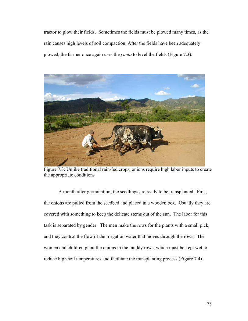
tractor to plow their fields. Sometimes the fields must be plowed many times, as the

rain causes high levels of soil compaction. After the fields have been adequately

plowed, the farmer once again uses the yunta to level the fields (Figure 7.3).

Figure 7.3: Unlike traditional rain-fed crops, onions require high labor inputs to create the appropriate conditions A month after germination, the seedlings are ready to be transplanted. First,

the onions are pulled from the seedbed and placed in a wooden box. Usually they are

covered with something to keep the delicate stems out of the sun. The labor for this

task is separated by gender. The men make the rows for the plants with a small pick,

and they control the flow of the irrigation water that moves through the rows. The

women and children plant the onions in the muddy rows, which must be kept wet to

reduce high soil temperatures and facilitate the transplanting process (Figure 7.4).

73

Figure 7.4: Transplanting is backbreaking work Photo taken by Toribio Maygua The distance between plants is approximately 10 cm, and the distance between rows

varies from 20 to 30 cm (Meruvia et. al. n.d.). Both sexes perform this task with

amazing proficiency, the men are able to work long hours making row after row, and

the women are extremely fast at pushing the thin stems into the wet ground. In

comparison with other local crops, such as maize, the tillage and planting

requirements for onions are much more labor intensive.

After the planting has been completed, the farmers must monitor field

conditions carefully. As the rainy season reaches its end in March, timely irrigation

of the early crop is essential. Several weeks after planting, the farmers begin the first

important weeding operation. Known in Quechua as the kachida, male workers use a

hoe to reshape the rows in which the onions were originally planted. The hoe is also

used to remove any emerging weeds. Some farmers will take this opportunity to

74

apply the first fertilizer treatment, usually a mix of Urea and commercial fertilizer

(18-46-00). In the following weeks after the kachida, the farmers will weed the field

a second time by hand. Both male and female laborers do this task.

Six to eight weeks after transplanting, the male laborers perform the most

labor-intensive task of onion farming, called the thamida in Quechua. This operation

involves the loosening of soil between the onion rows with a small pick. Weeds are

removed as the workers pass over weedy patches. Once this has been completed, the

farmers go back over the loosened soil with the same pick to recreate the rows that

were destroyed in the loosening process (Figure 7.5).

Figure 7.5: The brute force required for loosening the soil means that it is almost exclusively performed by men Photo taken by Toribio Maygua

75

It is at this time that the remaining amount of chemical fertilizer is applied to the

field, just before the digging occurs. Some farmers also apply chicken manure to the

onion crop at this point. Once this final mechanical operation has been completed,

the farmers’ primary concerns are timely irrigation to maintain adequate soil moisture

and fumigation to control insect pests and diseases.

As onion bulbs increase in size, photosynthate is transferred from foliage leaf

blades into storage leaves. Once this happens, the onion leaves begin to collapse.

This occurs 80 to 170 days after planting, depending on the cultivar. In the Tipajara

watershed, the farmers step on the falling leaves or roll them over with a 55-gallon

drum. This practice creates uniform conditions for the harvest. During the harvest

labor is divided by gender. Men dig the rows of onions with a pick and make piles of

the plants. The women and children cut the foliage from the onion and package the

bulbs in large sacks (Figure 7.6). This is a very labor-intensive process.

Figure 7.6: Harvesting onions

76

Figure 7.7 is a graphic depiction of the inputs required to produce an onion

crop, and the different actors involved in the production of the crop. The distinction

made between on-farm and off-farm inputs is important, and illustrates the extent to

which farmers are dependent on outside inputs and outside sources of capital. This

makes for a very undesirable situation when the farmer is unable to recover his

production costs

77

Figure 7.7: The primary inputs for onion production in the Tipajara watershed

78

INSECT PESTS AND DISEASES OF ONIONS

In the Tipajara watershed, the incidence of onion disease is determined by a

number of climatological variables, primarily annual rainfall, temperature, relative

humidity, and wind. Human behavior and farm management, however, greatly affect

the incidence of disease and the yield of the crop. Closely planted onions encourage

moisture and dew formation, which provides certain fungi with the perfect

microhabitat for reproduction and dispersal. Poor fumigation techniques can lead to

the development of resistant fungal strains. Most importantly, the lack of a

scientifically designed crop rotation scheme causes the year-to-year increase in

airborne fungal spores. The following is a synopsis of the diseases we have identified

in the community of Tipa Tipa. In May of 2001, Dr. Walter Kaiser, Peace Corps

plant pathologist, verified this information in the ITA laboratory in Sucre.

Downy mildew (Peronospora destructor) is one of the most serious diseases

affecting onion production in the region. The disease attacks onion leaves, especially

during periods of cool, moist weather, and causes serious losses in yield and bulb

quality. Initially, infected plants have extended, light green lesions along the length

of the leaf surface. In serious cases the fungus completely destroys the affected

leaves, which causes the plant to form new leaves, resulting in dramatically reduced

bulb size. The fungus remains dormant in onion plants, infected bulbs, and stored

seed. Infection is initiated during cool temperatures (less than 22ºC) and in the

presence of rain or dew on the leaf surface. Spore production occurs at night; newly

produced spores are then dispersed by wind during the day. Suggested methods of

control include destruction of contaminated crop residues, sufficient spacing between

79

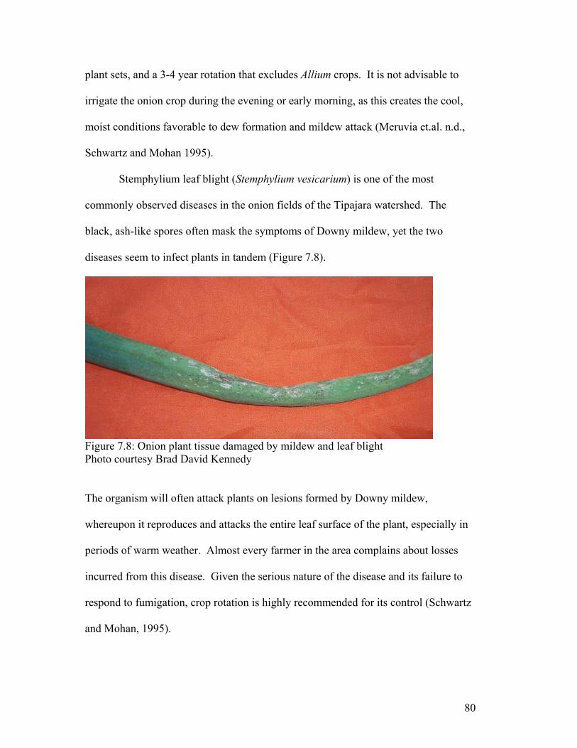
plant sets, and a 3-4 year rotation that excludes Allium crops. It is not advisable to

irrigate the onion crop during the evening or early morning, as this creates the cool,

moist conditions favorable to dew formation and mildew attack (Meruvia et.al. n.d.,

Schwartz and Mohan 1995).

Stemphylium leaf blight (Stemphylium vesicarium) is one of the most

commonly observed diseases in the onion fields of the Tipajara watershed. The

black, ash-like spores often mask the symptoms of Downy mildew, yet the two

diseases seem to infect plants in tandem (Figure 7.8).

Figure 7.8: Onion plant tissue damaged by mildew and leaf blight Photo courtesy Brad David Kennedy

The organism will often attack plants on lesions formed by Downy mildew,

whereupon it reproduces and attacks the entire leaf surface of the plant, especially in

periods of warm weather. Almost every farmer in the area complains about losses

incurred from this disease. Given the serious nature of the disease and its failure to

respond to fumigation, crop rotation is highly recommended for its control (Schwartz

and Mohan, 1995).

80

Cladosporium leaf blotch (Cladosporium alli-cepae) is a serious disease

affecting onions late in the cropping cycle. The defining symptom is a distinct

yellowing of the leaf area (Figure 7.9).

Figure 7.9: Onion crop at the onset of a Cladosporium attack Infected debris and infected seeds are most the most likely candidates for disease

transmission from year to year. Low temperatures (5-8.5ºC) and high humidity in the

absence of light encourage maximum sporulation. Plowing under of debris and

fumigation late in the cropping cycle are suggested methods of control (Schwartz and

Mohan, 1995).

Purple blotch (Alternaria porri) is commonly observed in the area. Although

not isolated under laboratory conditions, the unmistakable symptoms of this disease

81

make it easy to identify. Upon infection the leaf displays white, oval lesions that

quickly expand in a concentric fashion, becoming purple in the center as they do so

(Figure 7.10).

Figure 7.10: Typical lesions of Alternaria Photo courtesy Brad David Kennedy Favorable conditions for this disease are very similar to those for Downy mildew; it

reproduces at night in the dew formed on the leaf surface of plant sets. Daytime

temperatures in excess of 26ºC are favorable to the disease. It is dispersed by rainfall

and wind. As with other diseases, it can be controlled by destroying crop residues,

controlling the moisture on leaf surfaces, and through crop rotation (Meruvia et.al.

n.d.)

Pink root (Pyrenochaeta terrestris) is a disease causing fungus that lives in the

soil, sometimes at a depth of 45 cm, from where hyphae attack and penetrate root tips.

Pink root is most severe in fields where onions are planted for consecutive years. It is

possible to control the disease through soil fumigation, but considering the level of

technology and available capital in the area, this does not seem to be a feasible

solution. Again, crop rotation is the most advisable course of action to prevent the

82

disease from reaching epidemic proportions (Villarroel Leon 1997). The

recommended rotation is 3-6 years (Schwartz and Mohan 1995).

Thrips (Thrips tabaci) are the most commonly occurring insect pest attacking

onions in the Tipajara watershed. Thrips are extremely small, measuring 0.5 to 1.2

mm when immature, reaching a size of 2 mm when fully mature. Most thrips seek

refuge in the base of the leaves at the bottom of the plant. Adult thrips can fly.

Though onions and garlic are the preferred hosts, thrips can be found in cabbage,

cotton, celery, tomatoes, beans, cucumber and pineapple, and other weedy plants as

well. Thrips can complete the life cycle in 14 to 30 days; at temperatures above 30ºC

the life cycle is shortened to 10 or 11 days. Thrips feed by removing the green plant

tissue from the surface of onion leaves. The damage can reduce yields drastically, by

as much as 66% in some tropical countries. They can also act as a vector for

Alternaria, and the lesions and plant stress generated by thrips make the onion plant

more susceptible to attack by other pathogens. To reduce incidence of thrips, all

onion volunteer plants must be removed from the field, especially during periods

when onions are not being cultivated. Plants should be kept well watered and free

from other stresses such as nutrient deficiencies. A continuous presence of onion

plants, all the way from Mizque through the Tipajara watershed, means that thrips

constantly have a refuge in which they can reproduce and disperse (Rueda and

Shelton 1995)

Unaware of alternative disease control methods, farmers are increasingly

forced to rely more and more heavily on the use of chemical fungicides as a means of

control. Lack of proper equipment (e.g. masks, gloves, goggles, etc.) and poor

83

fumigation techniques pose a serious threat to human health. Resistance, moreover,

increasingly becomes a concern as farmers haphazardly spray chemicals without any

well-designed fumigation plan. It is certain that many diseases in the area, not just

those affecting onions, have already become resistant to chemical biocides. The

highest incidence of disease occurs when the onions begin to bulb. In most cases in

the Tipajara watershed, difficulties controlling disease results in a serious reduction in

crop yields.

ONION MARKETING AND POST-HARVEST TECHNIQUES

Once the onions have been harvested and bagged, onion farmers are primarily

concerned with getting their crop to market and the day-to-day fluctuations that occur

in the market price. Historical prices for onions are presented in Appendix II. Rivas

(2001, 2002) has argued that the primary constraints to profitability for onion farmers

in the valleys of Bolivia are poor post-harvest and marketing techniques. An analysis

of these arguments is necessary to fully understand the dynamics of onion production

in the Tipajara watershed.

First, it is important to realize that almost all farmers in the Tipajara watershed

apply no post-harvest techniques to improve the marketability of their crop. Farmers

do not cure their onions to increase the product’s shelf life. These uncured onions

have fresh, open wounds at the neck where the green foliage was cut from the bulb.

Such wounds, combined with poor handling techniques, cause the onions to decay

quickly once they have been loaded onto a truck for transport. Some onions will

sprout green foliage after only several days. Others will become infected by various

84

decay-causing organisms, which quickly rot the inside of the onion and make it unfit

for sale. The farmer has a small window of time in which to get his crop to market.

He is, therefore, more susceptible to fluctuations in the market price, as he does not

have the luxury of waiting until the price has reached a satisfactory level. To

compound this problem further, few farmers actually calculate the cost of production.

An onion will change hands many times from the moment it leaves the farm

until it arrives to the consumer’s household (Figure 7.11). In the Tipajara watershed,

there are two primary ways in which an onion crop is transported to the city. The

first, and most frequent, occurs when a transportista arrives in the community with a

heavy-load transport vehicle, called a camion in Spanish. This person knows which

communities offer which products at different times of the year. Often times the

transportista has already been in contact with the farmer via telephone. In other

cases, he will visit different farms and offer to buy recently harvested onions. In both

instances, the farmers are subject to the going market price. Though this leaves some

room for negotiation between the two parties, the farmer has a limited time in which

to sell because he is unable to store his crop. Sometimes the farmer transports the

crop himself, generally when a local camion owner is making a trip to a nearby city.

This is often the case when the farmer feels that he can get a higher market value by

paying the price of transport and negotiating a price in the city markets.

85

Figure 7.11: The market distribution network for onionsϮ

ϮThis figure shows percent increase of the product from the perspective of the farmer, representing a cumulative percent increase from the moment the product leaves the small farm.

86

From the rural farm, the onion crop has three major urban destinations:

Cochabamba (148 km), Sucre (187 km), and Santa Cruz (497 km) (Rivas 2001). The

province of Mizque has the benefit of being centrally located relative to these three

major urban centers. Variable market prices, city of origin, and road conditions are

just a few of the factors that determine the destination. Although each city market

functions according to different systems and norms, the underlying system from one

city to the next is quite similar.

Upon arrival to the city, the heavy transport vehicle goes directly to a central

market. In the central market the mayoristas are the first to buy the onions from the

arriving camion. In the Santa Barbara market of Cochabamba, for example,

approximately 15 mayorista women are the primary recipients of the arriving cargo.

The power that these women wield is expressed in a commonly repeated adage: “If

you don’t sell to them, you can sell once, but after that you can’t sell anymore.” This

rule also applies to buyers. The system is one of unwritten rules and social customs,

but is so effective that 100% of all camiones sell their product to the well-known

mayoristas (Rivas 2001). Though little is done in terms of packaging or selection, at

this stage the onions have an average price increase of 14% (Figure 7.11)

From here the onions might be directly sold to the menoristas, usually

indigenous women who sell a variety of agricultural products at low volume in

different markets around the city. Those who buy from the menoristas are usually the

consumers. In some cases, however, other middlemen will purchase the onions and

transport them to other markets at smaller quantities or even to other cities and towns.

87

These are known as rescatistas. In every instance, the product’s market price

escalates enormously relative to its original value at the farm level (Figure 7.11).

The unit price of an onion increases as it travels through this system for a

number of reasons. The menoristas are largely responsible for selecting the onions

according to size and for eliminating rotten and sprouting onions; in some markets,

however, the mayoristas are responsible for this task (Rivas 2001, Rivas 2002).

Losses incurred and time are compensated for by a higher market value. Also, we

must keep in mind that Bolivia is largely an agricultural society. A large peasant

population, mostly indigenous, relies on agriculture, in some form or another, for its

economic well-being. This elaborate distribution system is effective in two ways: it

distributes the product to the farthest corners of the country and it provides a

livelihood for thousands of people.

DIMINSHING RETURNS IN THE TIPAJARA WATERSHED

Fundamentally, low yields and high production costs are what make onion

farming such a difficult business for so many farmers. Though the law of

diminishing returns may have some exceptions, this is not one of them. Samuelson

(1967) gives this thorough definition of the law of diminishing returns:

An increase in some inputs relative to other fixed inputs will, in a given state of technology, cause total output to increase; but after a point the extra output resulting from the same additions of extra inputs is likely to become less and less. This falling off of extra returns is a consequence of the fact that the new “doses” of the varying resources have less and less of the fixed resources to work with.

This law holds true for all inputs, e.g. labor, fertilizer, and manure. Those farmers

that desire success must find a way to balance the costs of these inputs with the fact

88

that at some point, the crop will experience a reduced response to the applied input as

a result of diminishing returns. Many farmers have yet to realize this, as they believe

that constant fumigation will alleviate their problems with disease.

The problem of diminishing returns is exacerbated by the year-to-year

increase in disease causing organisms. The diseases that attack onions in the region

show no signs of disappearing. On the contrary, they have become more abundant

and more virulent with time. Fumigation and monoculture have become a tenuous

business for the small-holder farmer in the Tipajara watershed.

89

CHAPTER VIII: RESULTS AND DISCUSSION FOR ONION PRODUCTION

Onions are one of the most important crops in the Tipajara watershed.

Though a distant third to maize and potatoes in total land area cultivated, onions

account for 53.3 percent of the total volume of agricultural products in the province

of Mizque, compared with 5.2 percent and 19.7 percent for maize and potatoes

respectively (Ugarte 2001). Certainly they are the primary cash crop for most

families with irrigation for the six-month period during which they are cultivated.

The importance of this crop and the magnitude of the crisis in which most

onion farmers now find themselves was one of the primary factors that drove my

research interests throughout the course of my Peace Corps service. It is the goal of

this study to provide a detailed, quantitative description of this crucial component of

the farm system, and perhaps in the process discover some potential solutions to the

chronic problems of disease and profitability that plague the majority of farmers in

this region. Figure 8.1 shows irrigated parcels in Tipa Tipa during the month of July

2002, the same cropping season for which this study was performed. 45 hectares of

land had a crop cover at this time, most of which was certainly onions. Since the

cropping season of 2002 was unusually dry, less irrigation water meant an overall

reduction in total land area cultivated.

90

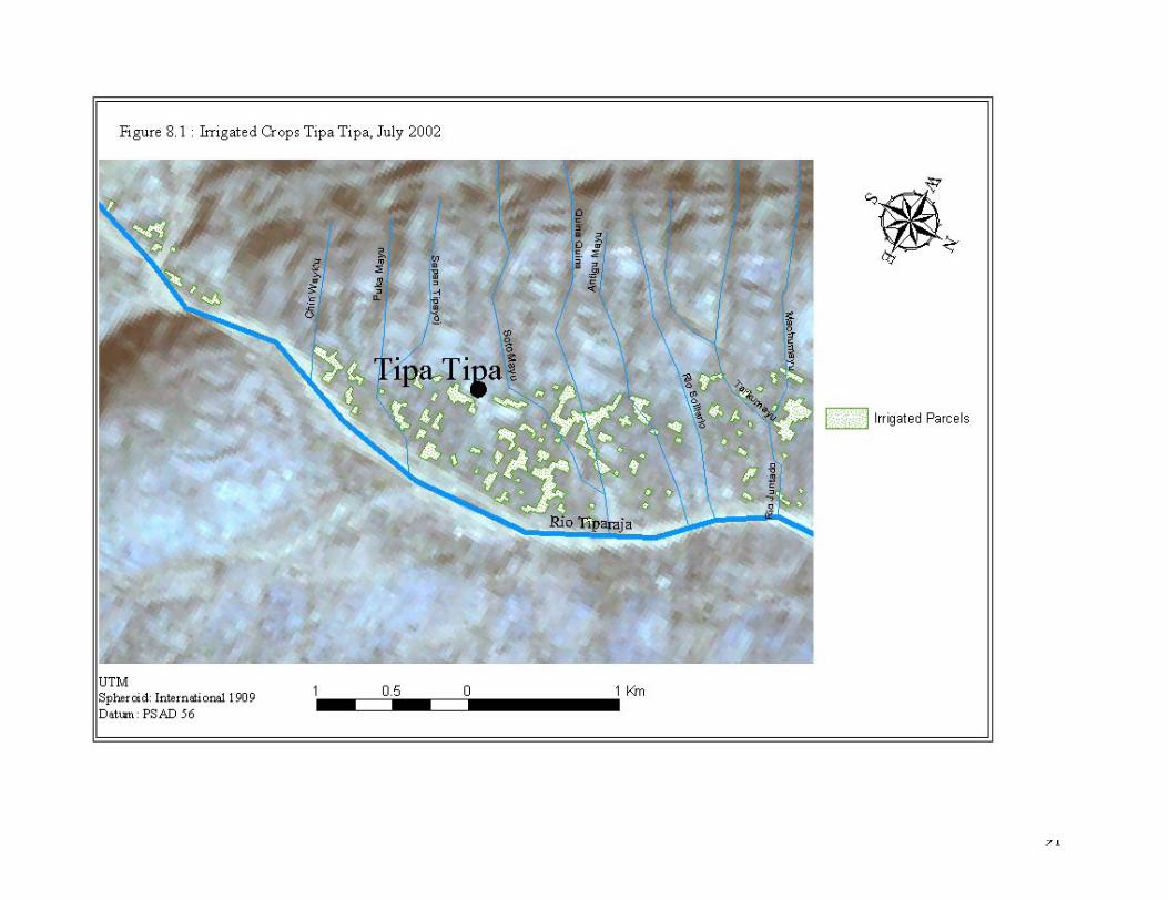
91

REGRESSION MODELS FOR YIELD

I used a multivariate regression analysis to measure the effect of changes in

inputs on yield (Hill, Griffiths, and Judge, 1997). The variables selected for this

final version of a yield model were selected based on several important criteria. I

made the logical assumption that only those variables directly related to the process

of onion production (i.e. inputs) would generate a practical, descriptive model of the

process. Further statistical analysis corroborated this assumption.

First, I eliminated all those measured variables that were not directly related to

onion production, such as the number of animals a farmer owns or the size of his

family. In most cases, these variables were not correlated with yield. Some variables

were combined with others; for example, female labor was combined with male labor

to create a total labor variable. Many of the variables in Table 8.1 were eliminated

from the regression model because the use of economic values, rather than quantities

(e.g. the difference between the cost of total labor and total labor days) yielded better

R2 values. This could be because the farmers themselves think in terms of economic

values. Relative prices may mean economic optimization uses a different set of

inputs than does physical optimization. Costs of N, P, and K were summarized in the

single variable of fertilizer cost. Table 8.1 shows the Pearson correlation

coefficients that were statistically significant but not included in the regression model.

92

Table 8.1: Pearson correlation coefficients with yield for variables not included in regression model Parameter Pearson Coefficient P ValuePrice per Bag 0.3888 <.0001 N 0.3353 <.0001 P 0.3649 <.0001 K 0.1748 0.0230 Labor Male 0.3163 <.0001 Days Male 0.3081 <.0001 Gross Income 0.9275 <.0001 Net Income 0.5675 <.0001 Days Female 0.2071 0.0069 Total Days 0.5477 0.0466 Tractor Hours 0.2319 0.0024 Oxen Days 0.2048 0.0076 Trucks of Manure 0.1931 0.0119

Based on my understanding of the farm system, I eliminated some variables

and combined other variables to create a final list of the variables to be included in

the equation. The resulting variables were consistent with my observations of the

significant inputs that the farmer invests in the production process. The following

regression equation had an R2 value of .38 and a Pr>F of .0001. The regression

equation is:

Yield (Tn/Ha) = 9.24 - 4.90(Parcel Size) - .0009(Total Labor/Bs/Ha) + .0026(Tractor/Bs/Ha) + .0084(Oxen/Bs/Ha) + .0011(Manure/Bs/Ha) + .0022(Seed) + .0051(Fertilizer) + .0008(Fumigation/Bs/Ha) + .0005(Irrigation Value)

93

Other important statistical indicators of statistical signficiance are included in Table

8.2.

Table 8.2: Variables for onion yield regression model Parameter Estimate P Value

Intercept 9.2436 0.0012 ParclSz (Ha) -4.9039 0.0112 TotLabor (Bs/Ha) -0.0009 0.1325 Tractor (Bs/Ha) 0.0026 0.2681 Oxen (Bs/Ha) 0.0084 0.0221 Manure (Bs/Ha) 0.0011 0.0036 Seed (Bs/Ha) 0.0022 0.1748 Fertilizer (Bs/Ha) 0.0051 0.0142 Fumigation (Bs/Ha) 0.0008 0.2919 Irrigation Value (Bs/Ha) 0.0005 0.0219

Table 8.2 shows that although not all values are significant in the equation as a

whole, a collinear relationship affects the statistical significance of several variables.

The Pearson coefficients of correlation show that collinear variables are correlated

with yield (Table 8.3).

Table 8.3: Pearson correlation coefficients with yield for variables included in regression model Parameter Pearson Coefficient P Value Parcel Size (Ha) -0.1849 0.0161 Total Labor (Bs/Ha) 0.2811 0.0002 Tractor (Bs/Ha) 0.1811 0.0185 Oxen (Bs/Ha) 0.1980 0.0099 Manure (Bs/Ha) 0.2697 0.0004 Seed (Bs/Ha) 0.3827 <.0001 Fertilizer (Bs/Ha) 0.4308 <.0001 Fumigation (Bs/Ha) 0.3364 <.0001 Irrigation Value (Bs/Ha) 0.0176 0.8485

94

Table 8.3 shows each variable correlated with yield, and all variables have a P value

that indicates statistical significance at the .10 level. So while some variables may

not contribute to the statistical power of the model because of collinear relationships,

each one has been chosen to create a logical, descriptive model for yield.

The variables that constitute the regression equation presented above represent

the fundamental inputs that the onion farmer in the Tipajara watershed uses to

optimize yield. The variables were generated from the original data set by calculating

a monetary value for each variable. Total labor takes the amount of days worked by

male workers and female workers and multiplies it by the market value for a day’s

labor for each gender. Tractor and oxen involve an almost identical conversion, the

difference for tractor being hours rather than days worked. It is important to note that

in many cases the farmers are not actually paying for the service provided. Figure 5.7

(page 41) provides a graphic depiction of those inputs that are on-farm compared with

those that are off-farm.

Many families own oxen, others do not and must rent them by the day, but the

maintenance costs for those families who own the oxen justify the inclusion of their

cost in the regression equation. Most families provide a good deal, if not the

majority, of on-farm labor that here has been included as an actual expense to the

farmer. Even though the farmers are not paying money for familial labor inputs,

these inputs must be included in the equation to achieve an accurate model of onion

production. The difficulty of measuring the amount of labor paid for versus the

amount of labor provided by family members precluded the quantification of these

two different values.

95

Fertilizer and fumigation values are outside inputs in every sense. The farmer

must pay for these with money, and if the farmer does not have cash readily available

he must seek credit from storeowners or moneylenders.

Seed is sometimes produced onsite, and other times it is purchased from other

farmers or companies which sell certified seed. In either case, attaching a monetary

value to onion seed is necessary, especially because quality onion seed has an

excellent value on the local market. Manure is another input that can be produced on-

farm, but many times a lack of animals dictates that the farmer purchase all or some

of the manure that is applied to the farm fields before the land is tilled. I know from

personal experience, the majority of manure that I have seen applied to onion fields

was chicken manure trucked in from the distant city of Santa Cruz. Those poor local

farmers who had significant quantities of goat or sheep manure often sold it to the

wealthier farmers engaged in the input intensive task of producing onions.

Although this yield model provides some clues regarding the relationship

between outputs and inputs, it is rather weak in explaining which farmers and which

practices are successful. I therefore found it necessary to distinguish between the

winners and the losers in the data set. I did this by simply looking at the net income

of each farmer; those farmers with a net income above zero I classified as winners,

and those farmers with a net income below zero were classified as losers. This

classification provides a much more compelling model of onion production.

The model for losers has an R2 value of .36 and a Pr>F of .0003. Table 8.4

lists all of the variables for the regression equation.

96

Table 8.4: Regression model for losing farmers Parameter Estimate P Value Intercept 5.9113 0.0362 Parcel Size (Ha) -2.2358 0.2014 Total Labor (Bs/Ha) 0.0001 0.825 Tractor (Bs/Ha) 0.0010 0.6335 Oxen (Bs/Ha) 0.0049 0.1518 Manure (Bs/Ha) 0.0006 0.2474 Seed (Bs/Ha) 0.0020 0.1944 Fertilizer (Bs/Ha) 0.0010 0.6761 Fumigation (Bs/Ha) 0.0005 0.5579 Irrigation Value (Bs/Ha) 0.0003 0.1953 It is important to notice that none of the included variables has a significant P value.

The model suggests that those farmers who lose money do not have a systematic

approach to onion production.

The regression model for those farmers who earn money is quite different.

The model has an R2 of .70 and a Pr>F of 0.0001. The variables are summarized in

Table 8.5.

Table 8.5: Regression model for winning farmers Parameter Estimate P Value Intercept 6.3889 0.1253 Parcel Size (Ha) -5.4892 0.0806 Total Labor (Bs/Ha) 0.0004 0.6424 Tractor (Bs/Ha) 0.0067 0.0915 Oxen (Bs/Ha) 0.0130 0.0172 Manure (Bs/Ha) 0.0009 0.0077 Seed (Bs/Ha) 0.0026 0.3033 Fertilizer (Bs/Ha) 0.0042 0.1097 Fumigation (Bs/Ha) 0.0012 0.2276 Irrigation Value (Bs/Ha) 0.0009 0.0094

97

The contrast between the two models is telling. The model for winners is much better

at explaining how farmers produce onions, which is indicated by an R2 of .70

compared to the losers R2 of .36. Moreover, several of the variables that were not

significant in the model for losers now become significant in the winner’s model.

Parcel size, tractor, oxen, manure, and irrigation value all have significant P values in

the winner’s model.

These striking differences suggest a very logical conclusion: farmers who earn

money are more systematic at balancing costs to optimize yields. Those farmers who

earn money behave in a more predictable, uniform fashion. Ultimately, it is the

management of the farm system that yields positive outcomes. The low R2 value for

the losers indicates that yield cannot be accurately estimated based on inputs, whereas

the reverse is true for the farmers that earn money. Here we must keep in mind the

law of diminishing returns and its impact on the farm system. For every household

each input has a different relative value. For example, a farmer with a large herd of

goats is unlikely purchase chicken manure to apply to his fields. The relative value of

chicken manure for this farmer is much higher because he already has a steady supply

of goat manure. So while the model does not indicate what the ideal proportions of

each input should be for each farmer, it does explain that the successful farmer is the

one that attributes the appropriate value to each input based on his unique situation.

Successful farmers are capable of thinking economically to balance costs and

optimize yields.

Surely there are other factors that were not measured that must affect yield,

such as soil type, microclimate, and access to credit, but we must keep in mind that

98

inputs and the management of those inputs are the single greatest factor that the

farmer has direct control over. And while soil texture and slope may have an effect

on yield, these physical constraints are much more difficult for the farmer to manage

and change.

Inevitably, we must address the question that arises when looking at these

models: How important is yield? Obviously the farmer wants to maximize his net

income, which doesn’t necessarily mean that he wants the greatest possible yield per

unit area. I have created a separate model for net income that provides some insight

into these basic questions. The regression equation is summarized below. It has an

R2 of 0.94

Net Income/Ha = -5979.84 - 1.02(Cost/Ha)

+ 481.12(Yield/Ha) + 110.96(Price/Bag)

The high R2 value is an outcome of the way in which net income was initially

calculated. Net income was not measured as a separate variable in the field, but

instead was calculated by multiplying yield per hectare times price per bag. The

resulting number was gross income; I then subtracted cost per hectare from gross

income, which is net income. The regression equation above does not conform to the

formal definition of a statistical model because the dependent variable was not

collected from field observations. It does, however, provide a useful tool for creating

a graphic representation of the relationship between the three variables that determine

net income. After developing this model, I used it to create several graphs to show

the relationship between the three primary variables that determine profitability: cost

99

per hectare, price per bag, and yield. These figures demonstrate the importance that

each of these variables has in the final outcome. They also show that the primary

factor driving profitability is yield.

These figures show income lines for different levels of yield, each figure

represents a different yield level. The income lines were created using the regression

model for net income described above. In each figure, there are two income lines.

The blue line represents net income at Bs. 3000/Ha; the green line represents net

income at Bs. 0, the break-even point. The points scattered within the diagram are the

actual data points for yields within 2.5 tn/ha of the yield indicated for the figure. The

figures show the effect that cost per hectare and price per bag have on net income at a

given yield. Any data points that occur below the blue line are instances where the

farmer made a profit of Bs. 3000 or greater. I selected the quantity of Bs. 3000 based

on my experience in the field; this is the minimum amount of money that a farmer

would like to earn for six months of labor. It is a conservative estimate, as I have

heard some farmers indicate that Bs.7000 would be the ideal amount. Naturally, as

price per bag increases the farmer has the option of incurring greater production costs,

thus the upward slope of the income lines. Any data points that occur below the

green line are instances where the farmer earned a positive return on onion

production. All data points that occur above the green line indicate that the farmer

lost money. Outliers were removed from the charts to facilitate comparisons between

them.

The relationship is clear: higher production costs at low yields make

profitability nearly impossible (Figure 8.2, 8.3). Even those farmers who sold onions

100

at a higher price per bag were unable to make a profit. As yield increases,

profitability becomes a greater possibility (Figures 8.4, 8.5). The graphs also indicate

that higher yields and their relationship to cost of production are more significant than

price per bag in determining which farmers make money and which farmers do not.

At higher yields, price per bag could be an important factor in causing the shift from

loser to winner.

Figure 8.2: Income Lines for Yield of 15 Tn/Ha

-2000

0

2000

4000

6000

8000

10000

12000

14000

0 20 40 60 80 100 120

Price/Bag (Bs.)

Cos

t/Ha

(Bs.)

@ Bs. 3000 @ Bs. 0

101

Figure 8.3: Income Lines for Yield of 20 Tn/Ha

0

2000

4000

6000

8000

10000

12000

14000

16000

0 20 40 60 80 100 120

Price/Bag (Bs.)

Cos

t/Ha

(Bs.)

@ Bs. 3000 @ Bs. 0

Figure 8.4: Income Lines for Yield of 25 Tn/Ha

02000400060008000

10000120001400016000

0 50 100 150

Price/Bag (Bs.)

Cos

t/Ha

(Bs. )

@ 3000 Bs. @ 0 Bs.

102

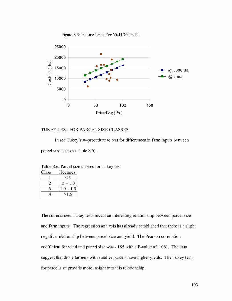
Figure 8.5: Income Lines For Yield 30 Tn/Ha

0

5000

10000

15000

20000

25000

0 50 100 150

Price/Bag (Bs.)

Cos

t/Ha

(Bs.)

@ 3000 Bs. @ 0 Bs.

TUKEY TEST FOR PARCEL SIZE CLASSES

I used Tukey’s w-procedure to test for differences in farm inputs between

parcel size classes (Table 8.6).

Table 8.6: Parcel size classes for Tukey test Class Hectares

1 <.5 2 .5 – 1.0 3 1.0 – 1.5 4 >1.5

The summarized Tukey tests reveal an interesting relationship between parcel size

and farm inputs. The regression analysis has already established that there is a slight

negative relationship between parcel size and yield. The Pearson correlation

coefficient for yield and parcel size was -.185 with a P-value of .1061. The data

suggest that those farmers with smaller parcels have higher yields. The Tukey tests

for parcel size provide more insight into this relationship.

103

Figures 8.6, 8.7, 8.8 and 8.9 show that farmers with smaller parcel sizes use

more total labor, more oxen, more seed, and more nitrogen per hectare than farmers

with larger parcels. The difference has the highest incidence of statistical

significance between the largest parcel size class and the smallest. Logically, Figure

8.10 shows that the smallest parcel size class has a per hectare cost of production that

is higher than the largest parcel size. Yields per hectare were also higher for the

smallest parcel size class as compared with the largest (Figure 8.11)

1 2 3 4 Figure 8.6 : Results of Tukey test (.05 confidence level) for difference in use of total labor (Bs/Ha) by parcel size class 1 2 3 4 Figure 8.7: Results of Tukey test (.05 confidence level) for difference in use of oxen (Bs/Ha) by parcel size class 1 2 3 4 Figure 8.8 : Results of Tukey test (.05 confidence level) for difference in use of seed (Bs/Ha) by parcel size class 1 2 3 4 Figure 8.9: Results of Tukey test (.05 confidence level) for difference in application of N (kg/ha) by parcel size class

104

1 2 3 4 Figure 8.10: Results of Tukey test (.05 confidence level) for difference in production cost (Bs/Ha) by parcel size class 1 2 3 4 Figure 8.11: Results of Tukey test (.05 confidence level) for difference in yield (Tn/Ha) by parcel size class

These results demonstrate that in smaller parcel sizes onion crops tend to receive

more inputs per hectare and hence have higher yields. The Tukey tests gave no

indication, however, that farmers with smaller parcel sizes have a higher net income.

It has already been established that yield is the main factor that determines

profitability in onion farming, and so it is therefore reasonable to conclude that

smaller parcel sizes yield better results. This is not to say that all farmers with small

parcel sizes earn money, for it has also been demonstrated that a failure to balance

costs with yield will always result in a net loss.

Rivas (2001, 2002), in collaboration with the technical team of FDTA-Valles,

proposes several improved post-harvest practices that have the potential to increase

the value of the onion crop at the farm level and to solve the problem of storage.

First, the farmers must cure the onions by placing them in long rows in the farm fields

and keeping them there for several days (Figure 8.12)

105

Figure 8.12: Curing onions in the field

At this time the translocation of photosynthetic material occurs, resulting in

the desiccation and yellowing of onion leaves and the enlargement of the bulb. This

operation allows the stem to form a scar, and facilitates the cutting of the stem and the

protection of the bulb from invasive pathogens. After cutting the stem, the onions are

then transferred to burlap sacks, where they will cure and dry for several more days

(Figure 8.13).

106

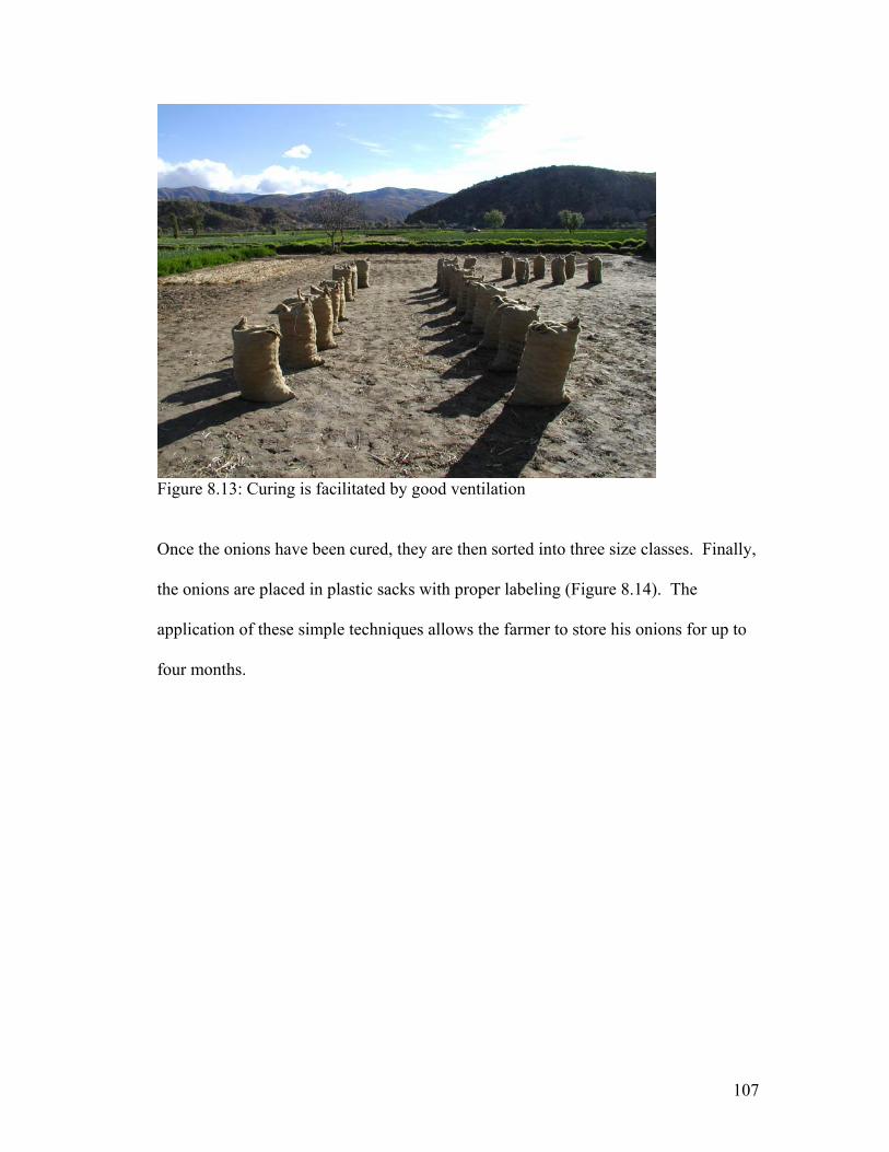
Figure 8.13: Curing is facilitated by good ventilation

Once the onions have been cured, they are then sorted into three size classes. Finally,

the onions are placed in plastic sacks with proper labeling (Figure 8.14). The

application of these simple techniques allows the farmer to store his onions for up to

four months.

107

Figure 8.14: Bags designed to improve marketing

These techniques are intended to form the basis of a larger marketing strategy

that seeks to improve the quality of the product and the negotiating power of the

small farmer in the larger market. Currently, FDTA-Valles is implementing this

project in the Tipajara watershed. Rivas (2001, 2002) assumes that these practices

will increase the value of the onion at the farm level instead of within the market.

The project hopes to create several cooperatives of onion farmers in several different

onion producing provinces in Bolivia. Rivas (2002) estimates that the farmers will

incur an additional cost of approximately Bs. 4,400/Ha to implement this technology;

increased costs can be attributed to the cost of burlap bags, increased labor costs, and

the cost of the mesh bags for transporting and selling the crop. It is also estimated

that the application of this technology has the potential to increase earnings by Bs.

7,000/Ha, though it is not specified if these are gross earnings or net earnings (Rivas

108

2002). As of January of 2003, however, these results had yet to manifest themselves.

Table 8.7 shows the price per bag in Bolivianos the participating farmers received

after applying the described technology. Comparing these prices to the price per bag

in Table 6.4 (page 43), it is readily noticeable that the average change in price is

negligible; in fact, it is below the average price per bag that a farmer receives selling

his crop in the traditional fashion.

Table 8.7: Price per bag and # of farmers applying improved marketing technology by size class of onions, Tipajara watershed Large Medium Small # of Farmers 32 38 38Average Price/Bag (Bs/Bag) 56.88 57.76 37.89Source: ACDIVOCA 2002

The data presented above was collected in the earliest phase of project

implementation. This information therefore provides no conclusive evidence

regarding the efficacy of this project, as these changes, if successful, will most likely

manifest themselves in the long-term. I have included this information because it

illustrates that even with improved marketing technologies, it is extremely difficult

for farmers in the Tipajara watershed to turn onion farming into a profitable

enterprise. In fact, any attempts at improved marketing will inevitably encounter a

certain degree of difficulty, mostly because the primary constraints to profitability

begin with production, and not, as FDTA-Valles has argued, with marketing.

Certainly the increase in price that the product experiences as it travels through the

chain of the market is considerable, and it is a worthy goal to introduce technologies

that will increase the bargaining power of the farmer vis-à-vis this complex network

of distribution. Nevertheless, the increased costs incurred and the apparent lack of

109

compensation with a higher market price could drive the most inefficient farmers

more deeply into debt. Selecting onions by size class, moreover, is actually a

disadvantage for those farmers that have generally low yields, as do the majority in

the Tipajara watershed. Selecting onions under these circumstances, when disease

has already decimated a crop, actually reduces the value of the product because the

farmer has willingly categorized the majority of his crop into the small category, the

lowest price class.

Many farmers in Tipa Tipa lamented the declining yields in onions and the

reduced response of disease to chemical controls. Among local farmers there was a

general consensus, disease had gotten much worse since the early days of onion

production. The cropping season of 2001 seemed to catch every farmer by surprise.

Never before had they seen disease attack their onion crop so severely. “There

wasn’t this much disease before,” was a phrase that I heard repeatedly from the local

farmers. One farmer, in an exasperated tone, once told me: “What are we going to do

about these diseases?” Another, explaining the disease to my Peace Corps project

coordinator who was visiting the community, had this to say: “We have such great

problems with onion diseases here, and they seem to be almost incurable.” A local

farmer, oblivious to the law of diminishing returns, became so desperate to control

disease that he prepared batches of fungicide in a 55-gallon drum, believing he could

out-muscle the organism with the brute force of quantity. So despairing had local

farmers become of the vicious cycle of fumigation and disease that a persistent rumor

began to spread that the disease was mixed in with the agrochemicals as a way to sell

more of the product. As Beets (1990) asserts: “…all continuous cropping with a

110

monoculture leads to problems. Most crops start to suffer excessively from pests and

weeds.” This is certainly the case in the Tipajara watershed (Figure 8.15).

Figure 8.15: Various diseases are destroying this onion crop Unfortunately, the farmers seem incapable of believing that the golden age of onion

production is over. Appendix II shows the zenith of this era, when in July of 1997 a

bag of onions was worth between Bs. 461 to Bs. 532.

111

CHAPTER VIII: CONCLUSIONS AND RECOMMENDATIONS

In this study, I have provided a detailed description of certain key components

of the farm system in the Tipajara watershed. I have documented the agricultural

intensification process that occurred after the Agrarian Reform of 1952, and I have

shown how increasing land fragmentation due to larger family sizes spurred the

introduction of irrigation technology in the community of Tipa Tipa. I have also

shown how national and local changes in infrastructure caused changes in village life

and the farming system. Agricultural intensification has done little to halt

environmental degradation; evidence suggests that intensification may accelerate

environmental degradation and have adverse affects on certain groups within the

community, e.g. women and the poor. A shrinking land base has resulted in high

levels of migration to urban areas, but future gains in production are still necessary if

the land is to sustain continued population growth.

Onions, one of the primary cash crops in the region, suffer from an epidemic

of disease causing organisms that drastically affect yields and thereby reduce the

possibility that farmers will make a profit. Within the population of onion farmers,

there are farmers that earn money and farmers that do not; those that do not earn

money are in the majority. The winning farmers were measurably different from the

losing farmers. Farmers that earn money are able to properly balance costs to

optimize yields and returns. For the vast majority of farmers, improvements in yield

have greater potential to improve profitability than improvements in marketing

techniques. Improved marketing techniques have the potential to increase the amount

112

of money a farmer earns, especially for those farmers that already have high yields.

Still, improved marketing techniques have not yet been proven effective in increasing

the average price per bag for onions.

The case for change is overwhelming. The current state of agriculture in the

Tipajara watershed is unsustainable. Chronic problems with disease and reduced

yields have driven many farmers to desperate and ineffective farming practices.

Environmental degradation continues through many channels: increased erosion,

deposition of toxic chemicals into the environment, and more deforestation. I have

written several recommendations that, if properly implemented, have the potential to

address many of the problems outlined in this thesis.

RECOMMENDATIONS

Realizing that different management strategies are necessary for different land

types, I have divided the lands of Tipa Tipa into three distinct categories based on

land cover and current use (Figure 7.8 page 64). Zone one comprises irrigated lands.

Zone two is hillside agriculture and extremely eroded lands. And zone three is forest

resources. Based on these divisions, I have made recommendations for each zone,

which could be used as the basis for future improvements in the farm system.

Zone One

This irrigated area is used primarily for the production of cash crops and for

the production of some staple crops. The primary objective of any agricultural

project in this zone should be crop diversification and the development of a

113

successful rotation scheme combined with an earnest attempt to reduce the total

cultivated area of onions. The evidence in this thesis is conclusive: smaller parcels

yield better results; crop rotation is imperative. This does not necessarily mean that

abandoning onions altogether is wise. As the statistical model for onions indicates, a

careful balancing of costs and the appropriate management of farm inputs greatly

improves the possibility of turning a profit. The reduction of total area cultivated has

numerous advantages:

1. Allows better management of a crop that is extremely input intensive

2. Improves the possibility of profitability

3. Makes more resources available for crop diversification

4. Facilitates control of disease

In the future, onions must be cultivated under an Integrated Pest Management (IPM)

scheme. Organic alternatives to chemical biocides exist and should be experimented

with. The destruction of volunteer plants, infected bulbs, and crop residues could

have an enormous impact on the year-to-year increase in airborne fungal spores.

Farmers could benefit greatly from learning the procedures for pesticide and

fungicide application. Learning about and understanding the life cycle of the causal

organisms will help farmers to combat them.

Agricultural technicians in India were able to reduce the cost of harvesting by

70% when using a simple, self-propelled onion digger windrower to perform the

mechanical operation of harvesting (Jadhav, Gharte, and Turbatmath 1995). Such a

technology has the potential to reduce the labor-intensive nature of the onion harvest

in rural Bolivia.

114

There is great potential to introduce intensive gardening techniques into zone

one. A move towards an organic, intensively managed polyculture would improve

family nutrition and provide a greater diversity of marketable crops. Such a risk

management strategy would mitigate the effects of fluctuating markets, natural

disasters, and disease epidemics.

Zone Two

Hillside lands are in desperate need of rehabilitation. These lands are

excellent candidates for the use of agroforestry and silvopastoral systems. Ideally,

these lands could be rehabilitated for the production of a number of useful products:

grazing paddocks, cut and carry fodder, wood products, and rain fed cereal crops.

There are also great opportunities for the construction of water catchments to expand

the area of irrigated agriculture. Foreign aid dollars will certainly be necessary to

subsidize the early rehabilitation process, as most local farmers have already

dismissed the idea of investing labor and time into these highly eroded areas. This

zone requires labor intensive soil conservation measures to halt the process of land

degradation. Both live and dead barriers have great potential to curb erosion. Ideally,

three dimensional GIS models would be used to develop a detailed management plan.

Zone Three

Due to the communal nature of these areas, it is extremely difficult to develop

a plausible management plan. Few forest trees remain on these steep slopes, as most

forest vegetation has been replaced by the shrubby pioneer species known as

115

chacatea (Dondonea viscosa). The soils that support this vegetation are generally

infertile, steep, and rocky. Goats and cows are commonly seen trampling through

these areas in search of the most palatable vegetation. Perhaps, as the PDAR (1991)

suggests, the best approach to managing these lands would be to leave them alone.

Priority should be given to the most intensively managed areas in the watershed, i.e.

zones one and two. Under ideal conditions and proper management, sustainable

practices in these zones could be adopted within 20 years. In the meantime, laws that

preserve remaining trees need to be enacted and enforced. Once sustainability has

been achieved in zones one and two, a province wide, landscape level approach to

forest management could be adopted. This approach would seek to promote natural

regeneration pathways using active fire management practices and relic forest trees as

a seed source. Such a project would require at least 50 years before the area began to

recover its original forest vegetation.

Unfortunately for Bolivians, conditions are far from ideal. Corruption is

rampant, local officials suffer from a chronic lack of resources, and many rural

community members have become disenchanted with agricultural development

projects that all too often deliver questionable results. Still, the campesinos never

ceased to amaze me with their extreme resiliency. Their acceptance of things as they

are struck me as both naively childish and impossibly wise. More than any single

thing, their talent to make something, however crude and rudimentary, out of almost

nothing, stands out in my mind. Surely such skill is grounds for optimism. I truly

believe that this skill is their key to a successful future. Only projects that seek to

enhance local innovation and build upon it will be successful in the future. This

116

requires an enormous investment of time and energy into the human resources that

exist at the rural level. For in the end, the development of human resources within

local contexts is the only real solution to global poverty.

117

Literature Cited

ACDIVOCA, 2002. Price data for two arroba bags of onions sold using the improved technology proposed by FDTA-Valles in the Tipajara watershed. Given to me by the ACDIVOCA director in the ACDIVOCA branch office of Mizque Beets, W.C. 1990. Raising and sustaining productivity of smallholder farming systems in the tropics. AgBe Publishing. Alkmaar, Holland. Bernard, H. Russell. 2002. Research methods in anthropology: qualitative and quantitative approaches, 3rd ed. AltaMira Press. Walnut Creek, California. Boa et. al. 2001. Técnicos as key informants. Economic Botany, Vol. 55(3): 363-369 Burrough, P.A., McDonnell R.A. 1998. Principles of Geographical Information Systems. Oxford University Press Inc. New York, New York. Caceras, S. 2003. Visited: 11/04/03. Movilización popular echó a Gonzalo Sanchez de Lozada. http://www.redvoltaire.net/article443.html Chang, K. 2004. Introduction to Geographic Information Systems. McGraw-Hill Companies Inc. New York, New York. CIA. 2003. Visited: 08/27/2003. The World Factbook: Bolivia http://www.cia.gov/cia/publications/factbook/geos/bl.html Crivelli, C. 1911. modified: 2003, visited: 09/16/03. The Catholic Encyclopedia, Volume XII. http://www.newadvent.org/cathen/12140a.htm Devereux, S., Hoddinott, J. 1993. Fieldwork in developing countries. Lynne Rienner Publishers. Boulder, Colorado. Distrito X de Salud de Mizque. data given to me August 2001 in Mizque, Bolivia. Freese, F. 1984. Statistics for land managers. Paeony Press. Jedburgh, Scotland. Gade, D.W. 1999. Nature and Culture in the Andes. The University of Wisconsin Press. Madison, Wisconsin. Godoy, R.A. 1984. Ecological degradation and agricultural intensification in the Andean highlands. Human Ecology. Vol.12 (4): 359-378 Hill, C.H., Griffiths, W.E., Judge, G.G. 1997. Undergraduate Econometrics. John Wiley & Sons, Inc. New York, New York.

118

Hudson, R.A., Handratty, D.M. 1989. visited: 10/23/2003. Bolivia a country study. http://lcweb2.loc.gov/frd/cs/botoc.html. IGM (Instituto Geográfico Militar). 2002. Atlas digital de Bolivia. CD-ROM INE (Instituto Nacional de Estadística). 2001. Censo nacional de población y vivienda. CD-ROM Jadhav R.V., Gharte, L.V, and Turbatmath, P.A. 1995. Design, development, and performance evaluation of onion digger windrower. Agricultural mechanization in Asia, Africa, and Latin America. Vol. 26 (3): 35-38 Klein, H.S. 1992. Bolivia: The evolution of a multi-ethnic society. Madison University Press. New York, New York. Knudson, J.W. 1986. Bolivia Press and Revolution 1932-1964. University Press of America Inc. New York, New York. Lagos, M.L. 1994. Autonomy and power: The dynamics of class and culture in rural Bolivia. University of Pennsylvania Press. Philadelphia, Pennsylvania. Larson, B. 1998. Cochabamba, 1550-1900: Colonialism and agrarian transformation in Bolivia. Duke University Press. London, U.K. Meruvia, Morales P. et. al. Manual de Cebolla. n.d. Enflex Ltda. Oruro, Bolivia. Nichols, P. 2000. Social survey methods: a fieldguide for development workers. Oxfam GB. Oxford, UK. Osman, A. Izquierdo, J., Galmarini, C.R. 1997. Regional onion short-day cultivar trial in Latin America and the Caribbean. Acta horticulturae. (433): 191-195 Pacheco, W.M. et. al. 1997. The mint of Potosi museum guide. Fundación Cultural del Banco Central de Bolivia. La Paz, Bolivia. Paulson, S. 2003. Gendered practices and landscapes in the Andes: The shape of asymmetrical exchanges. Human Organization. Vol. 62 (3): 242-254 PDAR (Programa de Ecología y Medio Ambiente). 1991. Estudio multidisciplinario de generación de datos base para el manejo y conservación de los recursos naturales de los rios Tucma, Callejas, Tipajara, Uchuchajra. Cochabamba, Bolivia. Unpublished. Given to me by Dr. José Salinas of Peace Corps Bolivia March 2001 Preston, D., Macklin, M., Warburton, J. 1997. Fewer people, less erosion: the twentieth century in southern Bolivia. The Geographical Journal. Vol. 163 (2): 198-205

119

Rivas, E. 2001. Descripcion Gral de la Cadena de la Cebolla en los Valles de Bolivia. Unpublished. Given to me by Marcos Moreno of FDTA-Valles June 2002. Rivas, E. 2002. Plan de Comercializacion de Cebolla Seca. Unpublished. Given to me by Marcos Moreno of FDTA-Valles June 2002. Rouma, G. 1933. Quitchouas et Aymaras. Extrait du Bulletin de la Societe Royale Belge d: Anthropologie et de Prehistoire. Brussels, Belgium. Rubatzky, V., Yamaguchi, M. 1997. World Vegetables: Principles, Production, and Nutritive Values. Chapman & Hall. New York, New York. Rueda, A., Shelton, A.M. modified: 1995, visited: 11/10/03. Thrips tabaci – IPM CIIFAD http://www.nysaes.maizeell.edu/ent/hortcrops/english/thrips.html Sachs, J. Morales, J.A. 1988. Bolivia 1952-1986. International Center for Economic Growth. San Francisco, California. Samuelson, P.A. 1967. Economics: An introductory analysis. McGraw-Hill Inc. New York, New York. Schwartz, H., Mohan, K., 1995. Compendium of Onion and Garlic Diseases. The American Phytopathological Society. St. Paul, Minnesota. SENAMHI (Servicio Nacional de Meteorología e Hidrología) n.d. climatological data for weather stations in Mizque and Aiquile for the years 1959-2001. Acquired from SENAHMI office in Cochabamba, Bolivia. Steel, R., Torrie, J., 1960. Principles and Procedures of Statistics. McGraw Hill Book Company, Inc. New York, New York. Swaney, D. 2001. Lonely Planet Bolivia. Lonely Planet. New York, New York. Ugarte, A.L. 2001. Plan de desarrollo de la primera sección municipal de la provincia Mizque. Unpublished. Given to me by Carlos Butron of the Mizque Comité de Vigilancia September 2001 Villarroel León, D., 1997. Manejo de Plagas: Tomo I. Universidad Mayor de San Simón. Cochabamba, Bolivia.

120

APPENDIX I: SOILS Translated from PDAR 1991

Order Entisols

Typic Ustorthents:

The characteristics of these soils in the study area are presented as follows.

They have no lithic contact within the first 50 centimeters. They are not saturated with water in the control section for more than 1 month out of the year. They have no cracks in the surface layer. They have thick textures that are very permeable, without any grade of compaction, and with a large amount of round and angular fragmented rocks. In the Tipajara watershed these soils represent a total surface area of 2,749 hectares, which is 11.2% of the total area. These soils are moderately deep with a texture ranging from loamy silt to loamy sand. They have a granular structure in the surface horizon without structure in successive horizons. External drainage is imperfect, while internal drainage is good. The parent material is alluvial. The soil pH ranges from 7.5 to 8.0, slightly to moderately alkaline. The electric conductivity in suspension fluctuates between .130 to .264 mmhos/cm. There is a slight concentration of salt, which is no problem in these soils. The cation exchange capacity is between 6.0 and 11.0 meq/100g. of soil. Total nitrogen content varies from .0009 a .0095%. Available phosphorus ranges from 1.2 to 2.8 p.p.m. Potassium content ranges from .12 to .38 meq/lt. Organic material falls between .18 and 1.95%, and is considered very low. These chemical characteristics, therefore, indicate low soil fertility. The riverbed in this watershed occupies a surface area of 320 hectares, which represents 1.4% of the total land area. Lithic Ustorthents*: These soils have all the characteristics of a Typic Ustorthent, except they posses a lithic contact within the first 50 cm. of the soil profile. These soils have a texture loamy to loamy sand, with structure in the entire profile. External drainage is excessive, and internal drainage is imperfect. Slopes vary between 25%-65%. Parent material is colluvial. The pH varies from 6.0 to 6.4, being slightly to moderately acid. They generally have a scarcity of macro-elements and no concentration of salts. The morphological characteristics of these soils indicate very low soil fertility.

121

Order Inceptisols Aridic Ustochrepts: These soils have all the characteristics of a Typic Ustochrept, except they are dry 6/10ths of the time during most years. These soils exist in the Tipajara watershed with a surface area of 1,992 hectares, representing 8.1% of the total area. They are deep soils with a sandy texture to a sandy clay loam. Soil structure is blocky sub-angular that go from weak to moderate, usually weak in the top horizon, moderate in successive horizons, without any structure at all in the lowest horizons. External drainage is imperfect, internal drainage is moderate. Parent material is alluvial. The pH varies from 6.2 to 6.9, slightly acid to neutral. Electrical conductivity fluctuates between .031 to .069 mmhos/cm, which shows that there are no significant concentrations of salts. The cation exchange capacity is between 8.4 and 9.9 meq/100 g., and is considered low. The percent of exchangeable sodium shows no adverse effects, as it is below 15%. Total nitrogen varies from .02 to .103%, which is considered low to moderate. Available phosphorus is between .4 to 1.3 p.p.m., which is also low. Potassium is between .18 and .46 meq/100 g., which is identified as moderate. Organic material varies from .97 to 2.06%, considered low. Chemical data from these soils indicates poor soil fertility in those soils located in the Tipajara watershed (Inceptisols). Order Alfisols Aridic Haplustalfs: These soils have all the characteristics of a Typic except they are dry for more than 6/10 of the year, in half or more than half of all years. These soils occur in the Tipajara watershed, representing a surface area of 4,137 hectacres, which comprises 16.9% of the total area. These soils are deep with a texture that ranges from silty clay loam to silty clay. The soil structure is in moderate sub-angular blocks in the surface horizon, and moderate to strong in subsequent horizons. External and internal drainage are both imperfect. The parent material is alluvial. The pH varies between 5.8 and 7.7, moderately acid to slightly alkaline. Electric conductivity in suspension fluctuates between .025 and 1.020 mmhos/cm., which is considered moderate in its concentration of salts. The cation exchange capacity is between 13.0 and 24.0 meq/100 g. of soil, which is considered moderate. The percent of exchangeable sodium fluctuates between 2.04%. This presents no significant problem as it is below 15%. Total nitrogen varies from .0001 to .0072%, which is identified as very low. Available phosphorus is from .5 to 17.2, high in the upper horizons and very low in the lower horizons. Potassium goes from .86 to 2.8 meq/lt., which is considered very high. Organic material is .12%, generally high in the upper horizons and very low in the lower horizons. These chemical characteristics indicate that these soils have a moderate to good fertility.

122

APPENDIX II: HISTORICAL PRICES FOR ONIONS

Onion Prices Mayorista Santa Cruz Market Jan Feb Mar Apr May Jun Jul Aug Sep Oct Nov Dec Avg.

1990 105.00 107.50 127.50 102.50 110.00 117.50 110.00 100.00 102.50 60.00 57.50 57.50 96.461991 42.50 40.00 40.00 40.00 60.00 75.00 75.00 95.00 137.50 147.50 112.50 82.50 78.961992 92.50 77.50 82.50 92.50 102.50 115.00 125.00 127.50 157.50 232.50 195.00 175.00 131.251993 125.00 125.00 125.00 132.50 142.50 80.00 80.00 147.50 117.50 127.50 67.50 77.50 112.291994 97.50 85.00 85.00 100.00 95.00 87.50 85.00 72.50 70.00 72.50 102.50 102.50 87.921995 122.50 120.00 92.50 100.00 87.50 182.50 160.00 117.50 100.00 82.50 90.00 82.50 111.461996 102.50 77.50 80.00 82.50 97.50 97.50 70.00 57.50 45.00 57.50 87.50 80.00 77.921997 122.50 160.00 162.50 242.50 292.50 345.00 465.00 302.50 180.00 110.00 102.50 77.50 213.541998 97.50 107.50 150.00 175.00 197.50 257.50 97.50 80.00 92.50 127.50 107.50 80.00 130.83

Source: Rivas 2001 Onion Prices Mayorista Cbba Market Jan Feb Mar Apr May Jun Jul Aug Sep Oct Nov Dec Avg.

1999 60.00 54.17 73.33 52.50 64.58 50.00 54.17 55.00 59.17 50.83 55.00 55.00 56.98 2000 93.33 83.33 66.67 66.67 72.92 87.50 106.67 70.83 108.33 54.17 91.67 100.00 83.51 2001 87.50 87.50 79.17 83.33 - - - - - - - - 84.38

Avg. 80.28 75.00 73.06 67.50 45.83 45.83 53.61 41.94 55.83 35.00 48.89 51.67 74.95

123

124

Onion Prices Mayorista Sucre Market

Jan Feb Mar Apr May Jun Jul Aug Sep Oct Nov Dec Avg.1998 80.00 70.00 120.00 195.00 120.00 300.00 120.00 360.00 40.00 160.00 140.00 80.00 148.75 1999 80.00 80.00 80.00 80.00 120.00 100.00 80.00 100.00 80.00 80.00 80.00 100.00 88.332000 100.00 180.00 180.00 140.00 160.00 140.00 160.00 120.00 100.00 100.00 100.00 80.00 130.002001 60.00 80.00 100.00 80.00 0.00 0.00 0.00 0.00 0.00 0.00 0.00 0.00 26.67

Source: Rivas 2001