Embed Size (px)
Citation preview
A Century of Land-Use Change in Metropolitan Phoenix
by
Kevin Kane
A Dissertation Presented in Partial Fulfillment
of the Requirements for the Degree
Doctor of Philosophy
Approved April 2015 by the
Graduate Supervisory Committee:
Breándan Ó hUallacháin, Chair
Abigail York
Aaron Golub
ARIZONA STATE UNIVERSITY
May 2015

© 2015 Kevin Kane
All Rights Reserved
i
ABSTRACT
The Phoenix, Arizona metropolitan area has sustained one of the United States’ fastest
growth rates for nearly a century. Supported by a mild climate and cheap, available land,
the magnitude of regional land development contrasts with heady concerns over energy
use, environmental sensitivity, and land fragmentation. This dissertation uses four
empirical research studies to investigate the historic, geographic microfoundations of the
region’s oft-maligned urban morphology and the drivers of land development behind it.
First, urban land use patterns are linked to historical development processes by adapting a
variety of spatial measures commonly used in land cover studies. The timing of
development – particularly the global financial crisis of the late 2000s, and the impact of
varying market forces is examined using econometric analyses of land development
drivers. This pluralistic approach emphasizes the importance of local geographic
knowledge and history to empirical study of urban social science while stressing the
importance of temporal effects. Evidence is found that while recent asset market changes
impact local land development outcomes, preferences for place may be changing too.
Even still, present-day neighborhoods are heavily conditioned by the market and
institutional conditions of the historical period during which they developed, while the
hegemony of low-cost housing on the urban fringe remains.

ii
DEDICATION
To my family.
iii
ACKNOWLEDGMENTS
First and foremost, I am heavily indebted to my co-authors for their part in the numerous
projects this dissertation involved. Without the intellect and hard work of Abigail York,
Joseph Tuccillo, John Connors, Chris Galletti, Yun Ouyang, and Lauren Gentile, the
published works that emerged from this dissertation – and, of course, the dissertation
itself – would not have been possible. I would also like to thank my supervisory
committee of Bréandan Ó hUallacháin, Abigail York, and Aaron Golub without whose
mentorship and patience with my stubbornness I would never have made it here. I was
fortunate enough to have the assistance of a great number of others from Arizona State
University’s School of Geographical Sciences and Urban Planning including Sergio Rey,
Elizabeth Mack, Xioxiao Li, B.L. Turner II, Mike Kuby, Scott Kelley, Joanna Merson,
and Jesse Sayles; those from other ASU units including David White, Ray Quay, Mary
Whelan, Sally Wittlinger, Skaidra Smith-Hesters; and those from outside the university
including Sandy Dall’erba, Richard Shearmur, and number of anonymous peer reviewers;
and others who I’m forgetting. Finally, I received financial and institutional support from
a number of organizations and funding sources including of course the School, Central
Arizona-Phoenix Long-Terms Ecological Research (NSF Grant #BCS-1026865), the
LTER network office, ASU’s Decision Center for a Desert City, and the Risk,
Perception, Institutions, and Water Conservation in Agriculture project (NOAA Grant
#NA11OAR4310123).
iv
TABLE OF CONTENTS
Page
LIST OF TABLES ................................................................................................................... ix
LIST OF FIGURES ................................................................................................................. xi
PREFACE........... ................................................................................................................... xii
CHAPTER
1 INTRODUCTION ................. …. ............................................................................... 1
1.1 Urban Arizona ..................................................................................... 1
1.2 Research Questions ............................................................................. 1
1.3 Methods and Conceptual Framework ................................................ 2
1.4 Dissertation Outline ............................................................................ 5
1.5 Summary ............................................................................................. 6
2 A SPATIO-TEMPORAL VIEW OF HISTORIC GROWTH .................................. 8
2.1 Introduction .......................................................................................... 8
2.1.1 Phoenix Urban History – A Background ........................... 12
2.1.2 Quantitative Urban Growth Analysis - Background ......... 14
2.2 Methods .............................................................................................. 16
2.2.1 Data and Spatial Extent ...................................................... 17
2.2.2 Quantity Disgreement ....................................................... 19
2.2.3 Allocation Disgreement ..................................................... 20
2.2.4 Spatial Relationships I: Join-Count Statistics ................... 21
2.2.5 Spatial Relationships II: Spatial Transition Matrices ....... 23
2.3 Results ................................................................................................ 24
v
CHAPTER Page
2.3.1 Quantity Disagreement: Phoenix Parcel Counts ............... 24
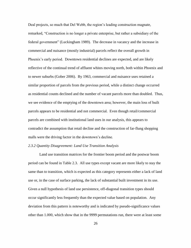
2.3.2 Quantity Disagreement: Land Use Transition Analysis .... 26
2.3.3 Allocation Disagreement: Pontius Transition Scores ........ 28
2.3.4 Spatial Relationships: Join-Count Statistics ...................... 30
2.3.5 Spatial Relationships: Spatial Markov Approach ............. 33
2.4 Discussions ......................................................................................... 36
2.5 Conclusions ........................................................................................ 38
3 BEYOND FRAGMENTATION AT THE FRINGE .............................................. 40
3.1 Introduction ........................................................................................ 40
3.2 Material and Methods ........................................................................ 45
3.2.1 Study Area .......................................................................... 45
3.2.2 Delineating Historical Periods .......................................... 47
3.2.3 Image Classification ........................................................... 50
3.2.4 Subset Images ..................................................................... 51
3.2.5 Spatial Metrics .................................................................... 52
3.2.6 ANOVA .............................................................................. 54
3.3 Results ................................................................................................ 55
3.3.1 Area and Density of Land Covers ...................................... 57
3.3.2 Fragmentation and Scatter .................................................. 59
3.3.3 Shape Complexity .............................................................. 60
3.3.4 Diversity ............................................................................. 61
vi
CHAPTER Page
3.4 Discussion .......................................................................................... 64
3.5 Conclusions ........................................................................................ 67
4 RESIDENTIAL DEVELOPMENT DURING THE GREAT RECESSION .......... 71
4.1 Introduction ........................................................................................ 71
4.2 Literature and Background ................................................................ 73
4.2.1 The Great Recession ........................................................... 73
4.2.2 Housing Supply: Developers and Zoning .......................... 76
4.2.3 Housing Demand: Individuals and Place ........................... 78
4.3 Empirical Setting ................................................................................ 79
4.3.1 Model specification ............................................................ 80
4.3.2 Data ..................................................................................... 81
4.4 Descriptive Results ............................................................................ 85
4.5 Residential Conversion Model Results ............................................. 93
4.5.1 Goodness-of-fit ................................................................... 93
4.5.2 Individuals and Demand .................................................... 96
4.5.3 Developers and Supply ..................................................... 101
4.6 Discussion ....................................................................................... 103
4.7 Conclusion ........................................................................................ 107
5 A SURVIVAL ANALYSIS OF LAND-USE CHANGE ...................................... 109
5.1 Introduction ...................................................................................... 109
5.2 Land Conversion Model .................................................................. 112
vii
CHAPTER Page
5.3 Study Area and Data ........................................................................ 116
5.3.1 Satellite Imagery and Agricultural Land ......................... 117
5.3.2 New Residential Construction ......................................... 119
5.3.3 Spatial Scale...................................................................... 119
5.3.4 Spatial Covariates ............................................................ 122
5.3.5 Institutional Covariates ................................................... 123
5.3.6 Housing Market ............................................................... 125
5.3.7 Agricultural Commodoties Market and Oil Prices .......... 126
5.4 Results and Discussion .................................................................... 127
5.4.1 Survival Curves ................................................................ 128
5.4.2 Functional Form ............................................................... 129
5.4.3 Cox Proportional Hazards Model Results ....................... 130
5.4.4 Main Effects – Spatial Covariates ................................... 130
5.4.5 Main Effects – Institutional Covariates ........................... 132
5.4.6 Main Effects – Market-Based Covariates ....................... 133
5.4.7 Lagged Main Effects ....................................................... 134
5.4.8 Interaction Effects ........................................................... 136
5.5 Conclusions ..................................................................................... 138
6 CONCLUSIONS .................. .................................................................................. 141
6.1 Key Findings .................................................................................... 141
6.2 Implications for Urban Research and Urban Theory ...................... 142
6.3 Policy Recommendations ................................................................ 146

viii
Page
REFERENCES....... .............................................................................................................. 148
APPENDIX
A SUPPLEMENTAL RESULTS FOR CHAPTER 5 ........................................... 162
ix
LIST OF TABLES
Table Page
2.1 Detailed Description of Land Use Categories ................................................... 18
2.2. Phoenix Parcel Counts by Category ................................................................... 25
2.3 Transition Matrices Showing Change in Land Use Category .......................... 27
2.4 Various Scores Described in Pontius et al. (2004) ............................................. 29
2.5 Observed and Expected Join-Counts with Simulated Significance Values ..... 31
2.6 Row-Standardized Spatial Markov Transition Matrices ................................... 34
2.7 Conditioned Staying Probability and Homogenization Probability ................. 35
2.8 Effect of Neighborhood Conditioning on Select Transition Types ................... 35
3.1 Basic Description of Spatial Metrics Used ........................................................ 54
3.2 ANOVA Pairwise Post-Hoc Tests for Landscape-Level Metrics .................... 57
3.3 ANOVA Pairwise Post-Hoc Tests for Class-Level Metrics ............................. 63
4.1 Housing Starts, State of Arizona ........................................................................ 74
4.2 Land Use Categories and Parcel Counts, 2002-2012 ........................................ 82
4.3 Parcels Transitioning to Single Family Residential Use ................................... 83
4.4 New Single Family Development by Urban Village ........................................ 89
4.5 Total and Mean Values for Transition-Eligible Parcels .................................... 91
4.6 Correlation between Zoning and Land-Use ....................................................... 93
4.7 Individual/Demand Logistic Regression Results .............................................. 95
4.8 Developer/Supply Logistic Regression Results ............................................... 100
5.1 NLCD Land Cover Categories ......................................................................... 118
5.2 Agricultural Cell Conversion at Multiple Resolutions .................................... 120

x
Table Page
5.3 Cox Proportional Hazards Model Results ....................................................... 129
5.4 Cox Model Hazard Ratios for Lagged Price Effects ....................................... 135
5.5 Hazard Ratios for Interaction Effects .............................................................. 136
xi
LIST OF FIGURES
Figure Page
2.1 The Expanding Boundary of Phoenix, Arizona ......................................... 11
2.2 Phoenix Parcels by Land Use Category ..................................................... 18
2.3 Phoenix Land Use by Category .................................................................. 25
2.4 A Graphical Rerepsentation of Pontius’ Metrics ....................................... 30
2.5 Selected Join-Counts ................................................................................... 31
3.1 Phoenix Block Groups by Dominant Construction Decade ...................... 49
3.2 Samples of Block Group Land Cover by Decade ...................................... 52
3.3 Boxplots of Landscape-Level Metrics ....................................................... 56
3.4 Proportion of Identified Landscape Cover Occupied by Each Class ........ 64
4.1 The Neighbors of Vacant Parcel 12024109 ............................................... 84
4.2 Single Family Residential Conversions in Phoenix ................................... 87
5.1 Maricopa County, Arizona Overview Map ............................................... 117
5.2 Agricultural Land Identified by NLCD (90m) ......................................... 119
5.3 Land Conversion at Three Resolutions (Avondale, AZ) .......................... 122
5.4 Survival Curves by Categorical Variables ............................................... 128
xii
PREFACE
I am not a native of Phoenix or of Arizona. I arrived here through one of the most
notable migratory pipelines between city pairs in the United States: Chicago to Phoenix.
Starting with wealthy entrepreneurs (the Wrigleys) and famous architects (Frank Lloyd
Wright) and continuing with less renowned sun-seekers, retirees and fans of Spring
Training baseball, this relocation is laden with Americana: the allure of the West and the
frontier, affordable homes, automobiles, and freedom from the crime, grime, and taxes
back east.
I have written on Chicago as well, an article in press at the Journal of Planning
Education and Research about a local development tool called tax increment financing.
Both cities could be described as pro-development despite their different political
landscapes. While in 2011 Arizona was the second state to designate an official state
firearm, it took a 2012 federal court order to make Illinois the 50th
state in the nation to
allow residents to carry concealed weapons in public. By 1915 Phoenix had ridded itself
of geographically-bounded city wards while ward bosses remain some of the most
powerful politicians in Chicago. Both, though, were built by boosters like Marshall Field
and the Goldwaters.
In Arizona, buttes and sunsets substitute for skyscrapers and lakefront. It may not
be as readily apparent in a city lacking iconic architecture, visually-distinct and
historically-embedded neighborhoods, and just one daily transatlantic nonstop, but the
Phoenix area is not, as some would have it, a “geography of nowhere.” It simply reflects
a shorter and more compressed development history resulting in less differentiation in
building stock, infrastructure, transportation type, and neighborhoods.
xiii
While knowledge of a place is a requisite of urban research, my interest and skill
lie in empirical, data-driven research on city development. As a child of two Chicago
architects and a one-time property tax professional in that city, it was issues of
development finance and urban sprawl in Chicago that first piqued my interest in
urbanism and motivated me to seek this PhD. Comparing the urban morphology of the
two cities is the first thing I did, though it’s harder to make your case using data than it is
to point at the lack of skyscrapers and commuter rail. Differences in data structure,
municipal and political fragmentation, and the power of large apparent differences
complicates between-city comparison of within-city pattern. This dissertation repeatedly
demonstrates that decisions on what to do with urban data are heavily conditioned by
regional peculiarities. Also, big differences dominate nuanced ones: empirical results
like average distance to transit, the impact of zoned density, or land cover diversity can
seem inconsequential if one city has double the population, is in a different region of the
country, or if one is New York and the other just isn’t.
I hope that some progress can be made by looking at replicable approaches such
as econometric modeling or what I call “historic, geographic microfoundations,” testing
them in one area with the benefit of local knowledge and keeping an eye toward future
comparative work. As so-called “big” data is increasingly sought by local governments
in order to improve policy and investment, they’ll need the local knowledge to
understand how to make it useful for their region and also the ability to look at how ideas
that originated outside their borders might be adapted for their own use.
1
CHAPTER 1
INTRODUCTION
1.1 Urban Arizona
The urban morphology of the Phoenix, Arizona metropolitan area is subject to a
lot of heavy-handed critique. It continually appears in the academic literature as a
cautionary example of what’s wrong with urbanism: a dismal early record of racial
inequality (Bolin, Grineski and Collins 2005), a lack of place and identity (Gober 2006),
degraded perceptions of quality of life (Guhathakurta and Stimson 2007), energy use,
urban sprawl, and environmental degradation (Ross 2011). Florida (2009) goes as far as
to describe Phoenix as a “giant Ponzi scheme,” with speculative real estate development
building on an economic base that is mainly comprised of – more speculative real estate
development. Some of these critiques are reflective of the emergence of the American
Sunbelt as an urban regime that is fast-growing, entrepreneurial in nature, and without a
clear raison d’être but faces increasing challenges over climate, air pollution, and traffic
congestion (see, e.g., Judd and Swanstrom 2008). Other critiques such as those over
water, the urban heat island effect, and municipal politics are more unique to
metropolitan Phoenix.
1.2 Research Questions
This dissertation investigates the historic, geographic microfoundations of
Phoenix’s (oft-maligned) urban morphology and the drivers of land development behind
it. Four individual analyses are conducted to investigate this overarching question in
more detail:
2
1. How did land use heterogeneity and complementarity develop in historic
Phoenix?
2. What does fragmentation – as it is used in discussions of urban sprawl – actually
mean; how does it vary in Phoenix based on when sub-metropolitan regions were
developed?
3. How did the global financial crisis of the late 2000s shift the locus of new single-
family home construction in Phoenix?
4. How is the urbanization of agricultural land in the Phoenix metropolitan area
dependent on not only on locational and institutional characteristics, but also
varying market conditions?
1.3 Methods and Conceptual Framework
This dissertation uses quantitative geographic and statistical methods to
understand land-use change in the Phoenix, Arizona metropolitan area while advancing
the use and application of these methods. Following Irwin and Geoghegan (2001) and
Irwin (2010), land change research conducted at the scale of an individual land parcel
directly links the observation unit with the decision-maker. Since urban land parcels
represent actual land ownership boundaries, observing a particular pattern of land parcels
connects the researcher to the processes behind their development. In landscape ecology,
for example, a spatial pattern such as fractal dimension might yield a meaningful
conclusion about an environmental process – species richness, for example. Similarly, a
city-wide pattern of parcels may give insight into the behavior of people and their impact
on the spaces they inhabit. Generally speaking, geographic pattern strongly informs the
social purpose of a built area (Talen 2011). While a structural economic approach could
3
model each landowner’s utility function in order to identify development drivers, this
approach runs the risk of losing the explicit connection between model observations and
specific units of land within the urban environment since characteristics of individual
owners are likely unavailable or obscured to protect privacy. Performing econometric
analysis at the scale of the data-generating process (i.e., the parcel-level or the best
available approximation) can identify key parameters undergirding a landowner’s
decisions especially in the short-term.
Chapters 2 and 3 of this dissertation deal with historic, geographic
microfoundations of urban development. They are concerned with understanding how
past trajectories yield current landscapes both explicitly by analyzing historical land use
data, and implicitly by considering present-day urban morphology based on when
neighborhoods were built. Whole-city spatial and space-time measures are used to
understand a variety of components of urban land-use change. Chapter 2 investigates the
relationship between four discrete land use categories to each other, following Kivell’s
(1993) observation that decline in one land use type (urban industry, in his example) can
lead to altered patterns in other sectors, namely an undesired interspersion of vacant,
residential, and remnant industrial land. Chapter 3 investigates the meaning of
fragmentation as it is used in debates over urban sprawl (Siedentop and Fina 2010). The
path-dependent nature of urban land is emphasized (Arthur 1988) whereby historic data
analysis can help to understand present-day conditions and present-day data can be used
to understand historic development trajectories. Metrics themselves vary; Seto and
Fragkias (2005) call for a diverse set of quantitative measurements to describe various
facets of urban growth. Statistics in this dissertation are necessarily tailored for specific

4
purposes. Chapter 2 uses join-count tests to understand changing spatial relationships
between land use categories and spatial transition matrices to infer the probability of
certain types of change such as persistence or homogenization probability. A suite of
methods called FRAGSTATS (McGarigal and Marks 1994) provides a wealth of
information about land cover patterns in Chapter 3.
Chapters 4 and 5 examine land-use change processes using a binary outcome
measure: whether land is developed or remains undeveloped. Using econometric
methodology, multivariate logistic regression and survival analysis techniques are used to
relate the instance of development to particular drivers including intraurban location,
zoning and institutions, neighborhood composition, demographics, and market
conditions. Chapter 4 investigates the contribution of these factors to the likelihood of
single-family residential development directly before and after the global financial crisis
of the late 2000s. Chapter 5 investigates the contribution of these factors to the
likelihood that agricultural land becomes developed into residential use from 1992 until
2014. Preferences for neighbors, demographic shifts, the effectiveness of zoning
regulations, the impact of infrastructure investment, and the impact of global financial
markets on whether parcels develop is investigated. While Chapter 4 is geared toward
specific shifts related to the global financial crisis including demography and
neighborhoods, Chapter 5 integrates an explicitly temporal modeling technique in order
to strengthen statistical identification.
Using multiple methods in this manner follows the bricolage approach suggested
by Sampson (2013), who argues that a single study or dependent variable isn’t sufficient
to capture all the aspects of neighborhood change in a city. Instead, a contextualist
5
approach is proposed using a combination of several outcome measures. This
dissertation’s methodological approach demonstrates techniques used for within-city
analysis while emphasizing that the choices made in how to understand data are heavily
conditioned by local context. These include a region’s development history, its physical
landscape, and the institutions that demarcate land as well as keep records of its use.
A component of these necessary choices, as illustrated by this dissertation, is the
question of how to define a city. Chapter 2’s historical focus restricts analysis to a small
area in Phoenix’s downtown core that was inhabited a century ago. While limited in
spatial extent, the original downtown core is emblematic of many of the broader concerns
about land-use change in the region. Chapters 3 and 4 use present-day boundaries of the
municipality of Phoenix. Phoenix is in fact the largest state capital in the US; in 2010 its
population of 1.45 million represented about 1/3 of the metropolitan area’s residents (US
Census 2010). Since the bulk of the region’s growth occurred during the time of the
private automobile and new land was continually annexed, the city of Phoenix’s density
gradient roughly mirrors that of the whole metropolitan area and includes a historic core
alongside suburban-style single-family homes, periurban areas, and undeveloped natural
land. In chapter 5 the analysis moves to the entire metropolitan region which is almost
fully bounded by Maricopa County.
1.4 Dissertation Outline
This dissertation relies on a compilation of four individual research papers on
land-use change in the Phoenix, Arizona metropolitan region. Chapter 1 is based on a
paper published with Abigail York, Joseph Tuccillo, Yun Oyuang, and Lauren Gentile in
Landscape and Urban Planning (2014). Chapter 2 is based on a paper published with
6
John Connors and Christopher Galletti in Applied Geography (2014). Chapter 3 is based
on a paper published with Abigail York, Joseph Tuccillo, Yun Ouyang, and Lauren
Gentile in Urban Geography (2014). Chapter 4 is based on a manuscript prepared with
Abigail York. In all cases, Kane is first author.
1.5 Summary
Understanding the spatial outcomes of driving forces of change in cities – namely
the aggregated location decisions of firms and households – can help municipal and
national level planners. On the local level, a better understanding of locational
preferences helps to understand the response to municipal land use institutions such as
zoning or development impact fees. While this dissertation only studies one metropolitan
area, Phoenix is emblematic of the American Sunbelt and other fast-growing regions that
are increasing in prominence and population worldwide. In particular, the region’s
fragile desert ecosystem, extreme temperatures, and heavily managed water and energy
landscape make it an excellent example for other cities concerned about sustainability,
sprawl, energy use, water availability, and climate.
Furthermore, empirical study of urban land-use change can provide verification or
reflection on commonly-held historical narratives or qualitative contentions about city
growth. Concerns over environmental justice are also prominent in the region (York et
al. 2014, Grineski, Bolin and Boone 2007), which has a historical legacy of marginalized
and spatially-concentrated populations that are disproportionately exposed to
environmental hazards. New Urbanists and proponents of compact growth often
emphasize the benefits of older cities in terms of walkability and land use
complementarity (Talen 2005, Jacobs 1961, Duany, Speck and Lydon 2010). The ideas
7
of compact growth can be sharpened by empirical analysis of historic cities, comparing
neighborhoods based on development timing, investigating the impact of
complementarity on development, or investigating the relationship between intraurban
location and transportation cost. Further, such analyses can be used to gauge whether
policies geared toward compact growth goals are working.
A final focus of this dissertation is achieving a spatially-explicit understanding of
cities over time. Land development represents the interplay between local demand for
productive places and the global market for investment capital. Developments are not
only durable and immobile, they also shape the experiences and fortunes of the people
who live and work there. The global financial crisis demonstrated a reciprocal effect
whereby broad distribution of local mortgage debt precipitated a crisis in the global asset
market, which then impacted neighborhoods in the form of foreclosures and stalled
growth. Conditions in global markets have wide-ranging impacts on place. Meanwhile,
and not entirely separately, preferences for place evolve over time. This dissertation
investigates these topics and the imprint they leave on urban form.
8
CHAPTER 2
A SPATIO-TEMPORAL VIEW OF HISTORIC GROWTH
2.1 Introduction
The historical morphology of cities is often described via narratives with rich
detail and thorough treatment of the peculiarities of each example. But there are also
strong quantitative traditions that characterize urban growth and form, such as Burgess’
concentric zone model that defined the Chicago School of urbanism (Park et al. 1925),
Adams’ model of urban transportation technologies (Adams 1970), and Batty’s cellular
automata growth models (Batty 2005). Quantitative approaches enable tests of widely
held narrative contentions about urban landscapes. More specifically, parcel-level
quantitative approaches connect individual land use decisions to the observed pattern of
urban and urbanizing landscapes, strengthening our understanding of the underlying
causal processes of land-use change (Irwin, Bell and Geoghegan 2003, Carrion-Flores
and Irwin 2004, Newburn and Berck 2006, Vaughan et al. 2005).
Lax annexation laws, ample land, and a post-World War II construction boom
fueled a unique Sunbelt morphology in Phoenix, Arizona (Gober 2006). This morphology
is characterized by sprawling, automobile-dependent suburban expansion and speculative
housing markets, contrasting with earlier eastern urban forms, which typically followed
Burgess’ or Adams’ growth patterns around a downtown core. Phoenix represents a 20th
century form of American urbanism described as rapid decentralized suburban growth
(Luckingham 1989), often at the expense of urban planning and environmental justice
issues (Bolin et al. 2005). It is often considered part of a new, Sunbelt urban regime that
is fast-growing and entrepreneurial in nature, but faces emerging challenges such as
9
climate, air pollution, and traffic congestion. The causal processes of change that
comprise this urban regime can inform development in regions with similar growth
trajectories as Phoenix (Guhathakurta and Stimson 2007, Keys, Wentz and Redman
2007). The city’s central business district (CBD), the original point of modern settlement
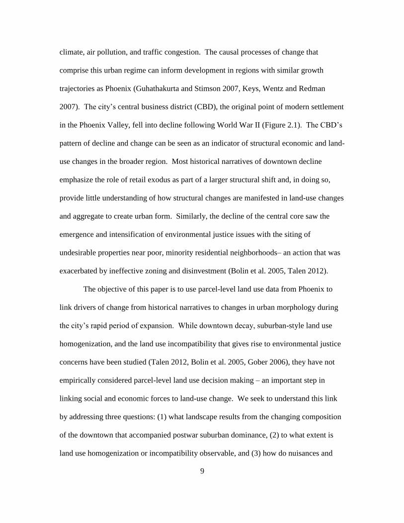
in the Phoenix Valley, fell into decline following World War II (Figure 2.1). The CBD’s
pattern of decline and change can be seen as an indicator of structural economic and land-
use changes in the broader region. Most historical narratives of downtown decline
emphasize the role of retail exodus as part of a larger structural shift and, in doing so,
provide little understanding of how structural changes are manifested in land-use changes
and aggregate to create urban form. Similarly, the decline of the central core saw the
emergence and intensification of environmental justice issues with the siting of
undesirable properties near poor, minority residential neighborhoods– an action that was
exacerbated by ineffective zoning and disinvestment (Bolin et al. 2005, Talen 2012).
The objective of this paper is to use parcel-level land use data from Phoenix to
link drivers of change from historical narratives to changes in urban morphology during
the city’s rapid period of expansion. While downtown decay, suburban-style land use
homogenization, and the land use incompatibility that gives rise to environmental justice
concerns have been studied (Talen 2012, Bolin et al. 2005, Gober 2006), they have not
empirically considered parcel-level land use decision making – an important step in
linking social and economic forces to land-use change. We seek to understand this link
by addressing three questions: (1) what landscape results from the changing composition
of the downtown that accompanied postwar suburban dominance, (2) to what extent is
land use homogenization or incompatibility observable, and (3) how do nuisances and
10
hazards become distributed as the city changes? In order to do so we draw on
quantitative traditions in urban growth modeling, ecological modeling, and spatial
analysis. First, we digitize and analyze Sanborn Fire Insurance Maps from 1915, 1949,
and 1963 to characterize land use in the CBD. Second, we use simple parcel counts and
transition matrices to measure the quantity of parcels in four broad land use categories
and their propensity toward certain types of change. Third, we sharpen our
understanding of transition types by measuring what Pontius, Shusas and McEachern
(2004) call allocation disagreement. Fourth, we explicitly model interactions between
parcels and their neighborhoods using join-count tests to determine how the changing
quantity or allocation of parcels changes their arrangement in space. Finally, we adopt a
spatial Markov chain approach to determine the propulsive influence of a parcel’s
neighbors on its likelihood of undergoing change.
The insights that emerge from this spatio-temporal analysis highlight the causal
processes of change that form urban landscapes. They also frame micro-level processes
and urban morphology as a cause and effect relationship. A better assessment of the
pattern and allocation of nuisance, hazard, or other incompatible uses in a rapidly
growing metropolis may also inform decision-making in regions around the world that
have similar growth trajectories as Phoenix. A historical approach to urban pattern is
especially useful. New Urbanist ideas about walkability and land use complementarity
are mostly derived from historic cities and continue to grow in popularity amongst
planners (Berke 2002, Talen 2005, Jacobs 1961). Planners and policymakers seeking to
increase the sustainability of urban neighborhoods and cities can utilize insights from
these quantitative parcel-level analyses instead of simply romanticizing pre-war urban
11
form. Rather than describing the past or attempting to model future growth, we conduct a
quantitative, historical analysis of one city that is emblematic of automobile sprawl,
seeking to observe how the past trajectory of parcels yielded a historic landscape so as to
better understand how current processes can yield future landscapes.
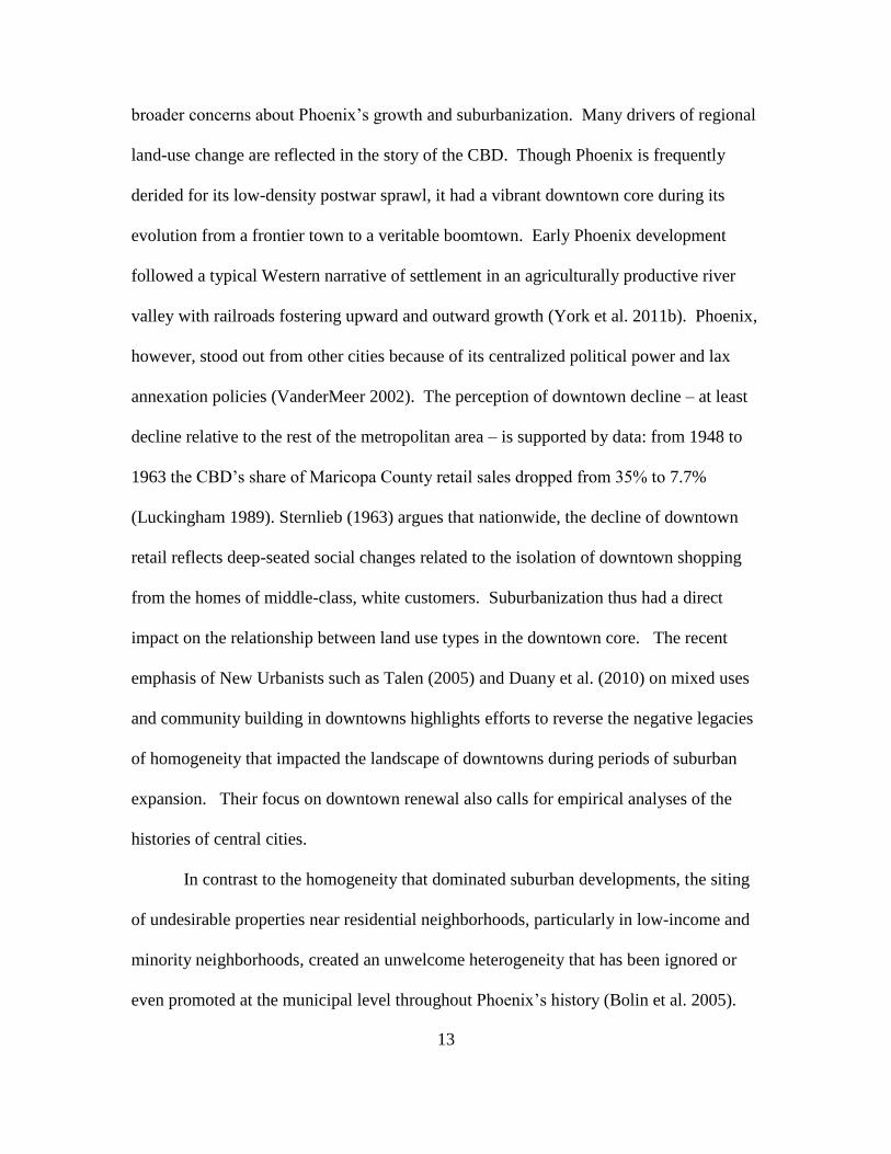
Figure 2.1: The expanding boundary of Phoenix, Arizona
12
2.1.1 Phoenix Urban History – A Background
Known as a booster-driven boomtown, Phoenix, while not even settled by
Westerners until after the Civil War, has maintained one of the nation’s highest urban
population growth rates for a century. However, it continually appears in the academic
literature as a cautionary example for what is wrong with urbanism: a dismal early record
of racial intolerance and inequality, a lack of place and identity (Gober 2006), degraded
perceptions of life quality (Guhathakurta and Stimson 2007), and the environmental
implications of sprawled development (Bruegmann 2005). Several aspects of these
historical narratives are inherently linked to urban morphology: Phoenix is known for its
polycentric urban development – rather than a single, strong core like older cities, it is
characterized by several functional subcenters that provide a measure of organization by
economic sector (Leslie and Ó hUallacháin 2006). Following early-century flooding, an
expansion of railroad-related industrial activity to the South, and an increase in the
availability of land, there was a notable residential shift as wealthier, white, non-Hispanic
residents gradually moved north while poorer, minority residents remained in South
Phoenix. Land use homogenization and land use incompatibility existed side-by-side, but
for different groups of people (Gammage 1999, Gober 2006). As the city’s functions
spread to subcenters and lower density outlying municipalities, the loudest complaints
have come from concerns over energy use (automobiles and air conditioning), landscape
degradation, and in broader and more recent vein, both weather and climate (Ross 2011).
This article focuses on a less explicitly (and less commonly) addressed concern
regarding the fate of the historic downtown central business district. Not only is the
dynamic of the CBD tractable at the parcel level, but it is also emblematic of many of the
13
broader concerns about Phoenix’s growth and suburbanization. Many drivers of regional
land-use change are reflected in the story of the CBD. Though Phoenix is frequently
derided for its low-density postwar sprawl, it had a vibrant downtown core during its
evolution from a frontier town to a veritable boomtown. Early Phoenix development
followed a typical Western narrative of settlement in an agriculturally productive river
valley with railroads fostering upward and outward growth (York et al. 2011b). Phoenix,
however, stood out from other cities because of its centralized political power and lax
annexation policies (VanderMeer 2002). The perception of downtown decline – at least
decline relative to the rest of the metropolitan area – is supported by data: from 1948 to
1963 the CBD’s share of Maricopa County retail sales dropped from 35% to 7.7%
(Luckingham 1989). Sternlieb (1963) argues that nationwide, the decline of downtown
retail reflects deep-seated social changes related to the isolation of downtown shopping
from the homes of middle-class, white customers. Suburbanization thus had a direct
impact on the relationship between land use types in the downtown core. The recent
emphasis of New Urbanists such as Talen (2005) and Duany et al. (2010) on mixed uses
and community building in downtowns highlights efforts to reverse the negative legacies
of homogeneity that impacted the landscape of downtowns during periods of suburban
expansion. Their focus on downtown renewal also calls for empirical analyses of the
histories of central cities.
In contrast to the homogeneity that dominated suburban developments, the siting
of undesirable properties near residential neighborhoods, particularly in low-income and
minority neighborhoods, created an unwelcome heterogeneity that has been ignored or
even promoted at the municipal level throughout Phoenix’s history (Bolin et al. 2005).
14
Kivell (1993) notes the role played by postwar industrial decline in changing urban
landscapes. Changes in one sector – industrial, in his example – lead to altered patterns
of land use in other sectors such as housing and utilities. This creates a haphazard land
use pattern with remnants of industry interspersed with some housing and a high quantity
of vacant or public open space, as the rate of commercial or industrial decay often
outpaces the ability of a city economy to absorb non-wealth producing land. Again, a
structural economic change drives a change in the relationship between different land use
types in a city, though in this instance the result is land use incompatibility. The lack of
effective institutional controls on land use and capital outflow within an area in a rapid
state of flux such as postwar Phoenix may yield an urban landscape where lower order,
industrial uses create a nuisance for nearby higher-order residential or retail uses. This
contention is congruous with Phoenix’s environmental justice and downtown decay
narratives and underscores the importance of understanding the spatial distribution of
nuisances and hazards as the city changes.
2.1.2 Quantitative Urban Growth Analysis – Background
While some urban researchers utilize a historical narrative approach based upon
qualitative evidence (see Kallus (2001), for example), quantitative analysis of intraurban
form has a rich history dating back to von Thunen’s nineteenth-century concentric model
to explain location rent (von Thunen 1966). The Chicago School of urban sociology
extended this method to city growth patterns during the 1920s, while further models such
as Adams (1970) incorporated transportation-based growth. More modern,
computationally-intensive models have been led by cellular automata and agent-based
modeling, which combine an initial state of land use with a set of decision rules to predict
15
urban growth outcomes (Batty 2005). In addition, econometric models have been used to
estimate determinants of rural land conversion at the urban fringe (Carrion-Flores and
Irwin 2004), while metrics like patchiness and fractal dimension have also been
developed to characterize the extent and form of urban land conversion (Seto and
Fragkias 2005). Remote sensing and ecological models are particularly promising for use
in analyzing urban land conversion (Verburg 2004). Pontius (2000), Pontius et al.
(2004), and Pontius and Millones (2011) provide a generalizable land use transition
framework that relies on a series of transition matrices between land use categories to
measure both the quantity and allocation of populations, thereby sharpening the grasp on
landscape change processes by including measures of persistence, loss, gain, and swap.
Pontius proposes decomposing landscape change into quantity disagreement and
allocation disagreement: the former representing the amount of mismatch due to different
populations in each category and the latter showing the difference as observed on a map
due to changing spatial allocation of the categories (Pontius and Millones 2011).
Geographical models that explicitly model spatial relationships can also be used
to quantitatively assess urban landscape change, which follows from an interest in
geographic statistics dating back to the 1960s. Join-count tests, first introduced by Dacey
(1965) and refined by Cliff and Ord (1973), quantify the number of instances that two
phenomena exist near each other in space. Join-counts can be used in a wide variety of
contexts to analyze spatial autocorrelation in terms of deviation from a random, expected
value or in terms of how the spatial relationships between observed phenomena change
over time. Bell, Schuurman and Hameed (2008) use join-count tests to determine
whether occurrences of non-accidental injuries are spatially autocorrelated based on
16
whether they are significantly different from an expected value, while Rey, Mack and
Koschinsky (2012) use join-counts over time to analyze the changing spatial patterns of
residential burglaries. Vaughan et al. (2005) create a measure of proximity similar to
join-counts for historic geographic data from London which is used to determine how
spatial segregation varies by income class.
Wood et al. (1997) propose a spatial Markov approach for land-use change
modeling, suggesting that land use transitions can follow a first-order Markov process.
Rey (2001) provides a number of methods whereby spatial dependence can be integrated
into a Markov chain transition matrix framework. Neighborhood conditioning asks how
the likelihood of transitioning from one income class to another depends on the income
class of your neighbors, defined (somewhat arbitrarily) as spatial units sharing a common
boundary or vertex. This allows the researcher to determine whether the likelihood of
transitioning from one category to another differs in the presence of certain neighbors.
This approach can provide insights into the emergent properties of Phoenix’s urban
landscape such as trends toward homogenization, mixing of uses, or land use
incompatibility. Spatial analytic approaches are particularly well suited to understanding
how parcel-level land-use changes impact urban morphology.
2.2 Methods
The objective of this paper is to provide an empirical, parcel-level analysis of
land-use change in Phoenix and compare these findings to drivers of change from
historical narratives. It addresses quantity disagreement, allocation disagreement, and
spatial outcomes at the finest possible resolution using four approaches described below,
which are drawn from quantitative traditions in urban growth modeling, ecological
17
modeling, and spatial analysis. Using these methods, this paper addresses three questions
about which parcels are changing and in what way: (1) what landscape results from the
changing composition of the downtown that accompanied postwar suburban dominance,
(2) to what extent is land use homogenization or incompatibility observable, and (3) how
do nuisances and hazards become distributed as the city changes? This empirical
approach may be used as a model for researchers interested in better understanding
dynamic urban regions in the past and today.
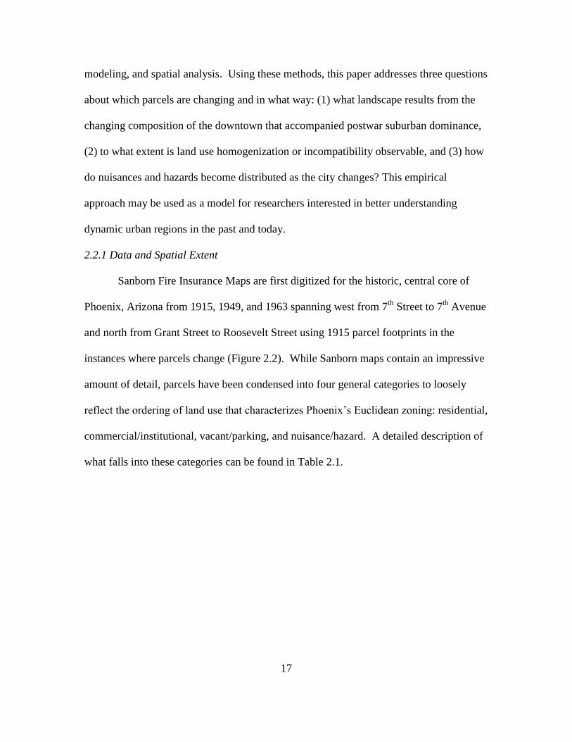
2.2.1 Data and Spatial Extent
Sanborn Fire Insurance Maps are first digitized for the historic, central core of
Phoenix, Arizona from 1915, 1949, and 1963 spanning west from 7th
Street to 7th
Avenue
and north from Grant Street to Roosevelt Street using 1915 parcel footprints in the
instances where parcels change (Figure 2.2). While Sanborn maps contain an impressive
amount of detail, parcels have been condensed into four general categories to loosely
reflect the ordering of land use that characterizes Phoenix’s Euclidean zoning: residential,
commercial/institutional, vacant/parking, and nuisance/hazard. A detailed description of
what falls into these categories can be found in Table 2.1.
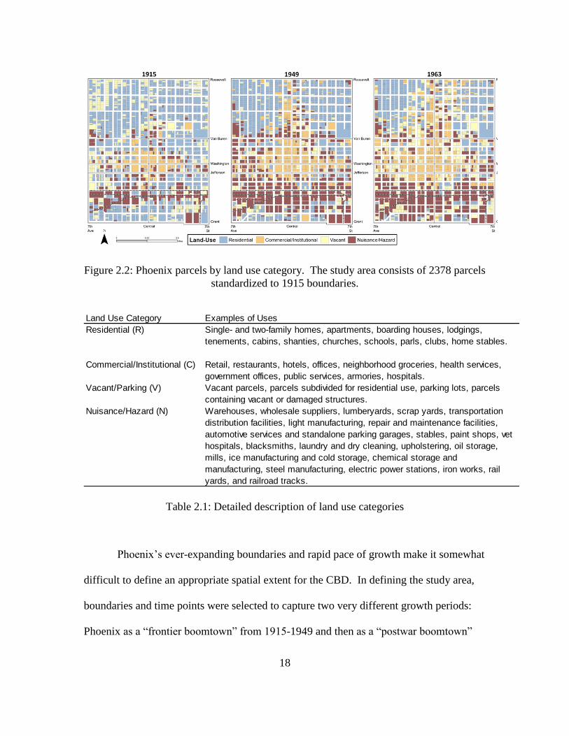
18
Figure 2.2: Phoenix parcels by land use category. The study area consists of 2378 parcels
standardized to 1915 boundaries.
Table 2.1: Detailed description of land use categories
Phoenix’s ever-expanding boundaries and rapid pace of growth make it somewhat
difficult to define an appropriate spatial extent for the CBD. In defining the study area,
boundaries and time points were selected to capture two very different growth periods:
Phoenix as a “frontier boomtown” from 1915-1949 and then as a “postwar boomtown”
Land Use Category Examples of Uses
Residential (R) Single- and two-family homes, apartments, boarding houses, lodgings,
tenements, cabins, shanties, churches, schools, parls, clubs, home stables.
Commercial/Institutional (C) Retail, restaurants, hotels, offices, neighborhood groceries, health services,
government offices, public services, armories, hospitals.
Vacant/Parking (V) Vacant parcels, parcels subdivided for residential use, parking lots, parcels
containing vacant or damaged structures.
Nuisance/Hazard (N) Warehouses, wholesale suppliers, lumberyards, scrap yards, transportation
distribution facilities, light manufacturing, repair and maintenance facilities,
automotive services and standalone parking garages, stables, paint shops, vet
hospitals, blacksmiths, laundry and dry cleaning, upholstering, oil storage,
mills, ice manufacturing and cold storage, chemical storage and
manufacturing, steel manufacturing, electric power stations, iron works, rail
yards, and railroad tracks.
19
from 1949-1963. By 1915, a variety of events had set the stage for growth and change in
urban form, including the completion of the Roosevelt Dam, a move away from a
geographically-elected city council, and early adoption of automobile transportation
(Luckingham 1989). By 1949, the so-called Valley of the Sun had grown steadily,
augmenting its reputation as a desert oasis with huge amounts of federal investment from
the New Deal and World War II. By 1963, substantial demographic shifts began to
change the residential arrangement of the Phoenix Valley toward one of tract homes
farther from the city. This was due in part to Federal Housing Authority subsidies that led
to the creation of so-called “developer suburbs” (Gammage 1999). The downtown core
remained largely static between the late 1960s and the most recent period of urban
renewal in the 1990s and 2000s, during which time the bulk of the region’s growth and
change took place outside the CBD.
2.2.2 Quantity Disgreement
First, quantity disagreement between land uses is observed by simply counting the
parcels and using row-standardized transition matrices, displaying the number of parcels
N in each category i at time t0, then comparing to Nj at time t1. This follows the
foundation of a hazard of change approach taken by Irwin et al. (2003). The number of
parcels that undergo a transition from category i to category j is denoted as Nij. The row-
standardized transition probability Pij is the proportion of parcels that are in category j at
t1 for each category i in t0. The expected number of parcels experiencing each transition
type Nij is given by Eij
𝐸𝑖𝑗 = 𝑁𝑖 × 𝑁𝑗
𝑇
20
where Ni is the number of parcels in category i at t0, Nj is the number of parcels in
category j at t1, and T is the total number of parcels in the study area (2378). Eij is
referred to as the population-predicted value. A pseudo-significance p-value based on
series of random permutations of land use is also calculated:
where m is the number of permutations in which the observed transition count is greater
than the expected value and n is the total number of permutations.
2.2.3 Allocation Disgreement
Next, allocation disagreement is observed using Pontius’ metrics for persistence,
gain, loss, and swap, providing a formal metric for spatial allocation changes that might
be casually observed on a map. Statistical analysis of land use transitions is complicated
by the fact that each transition type represents only a portion of a joint distribution.
Pontius et al. (2004) suggest that the classical, statistical method for analyzing land-use
change would be to generate an expected value based on populations, then use a chi-
square test to determine if the entire distribution is significantly different from random –
a relatively useless exercise because “scientists usually already know that persistence
dominates the landscape” (Pontius et al. 2004). The persistence score is born out of the
idea that there can be a change in the locational distribution of parcels of a certain
category even if their count is the same in both periods. Thus, a parcel that “persists”
exhibits the same use in both periods, while a “gain” parcel transitioned into that category
over the time period and a “loss” parcel left the category. For example, a residential
neighborhood may be demolished – say, in the case of Phoenix’s Chinatown – and
another one built elsewhere. In this hypothetical, the loss in residential is equal to the
𝑝 = 𝑚 + 1
𝑛 + 1
21
gain. The extent to which gain and loss offset each other (formally, the absolute value of
the difference) is called “swap” and indicates a shifting allocation of parcels.
2.2.4 Spatial Relationships I: Join-Count Statistics
Next, spatial relationships are modeled with join-counts to measure the likelihood
of particular use types existing in close proximity. Though gain, loss, and swap metrics
can indicate that a use type is moving, they provide no detail as to where this may be
happening nor do they offer any insights about the resulting spatial arrangement of the
urban landscape. Since the social purpose of the built environment can be strongly
informed by geographic pattern (Talen 2011), join-counts are an appropriate method for
analyzing the neighborhood-level effects of parcel land-use change by quantifying the
homogeneity or compatibility of land uses in an area.
The classic way to define a join is if two polygons have a boundary of positive
nonzero length in common (Cliff and Ord 1981). However, parcels in a GIS environment
do not achieve contiguity because parcels across the street do not share a boundary and
would not be identified as neighbors. A set of k nearest neighbors or a threshold distance
based on parcel centroids is insufficient as well. Many parcels in Phoenix are more than
twice as long as they are wide, resulting in two parcels over being considered a neighbor
before the parcel across the street is identified. Heterogeneity in parcel size and street
width preclude a centroid-to-centroid threshold distance from being meaningful because
of its tendency to miss joins involving large parcels. To circumvent these problems we
draw a 200-foot buffer around the boundary of each parcel and identify any other parcel
with portions lying within the buffer to be the target parcel’s neighbor. Using this spatial
weights scheme, parcels in the study area have between 4 and 43 neighbors with a mean

22
of 20 and a standard deviation of 4.27. This distance – and the resulting number of
neighbors – is intended to measure what a person might see and feel when she walks out
the front door rather than providing a measure of accessibility or accounting for the effect
of adjacent parcels only.
Join-counts are most commonly used in a binary (B = black and W = white)
situation in which the three possible outcomes are BB, WW, and BW, with the first two
representing positive spatial autocorrelation. Examples using more than two categories
are rare, though Zhang and Zhang (2008) explore the six unique join types that would
result from a trinary scheme: black, white, and grey. The use of four land use categories
results in ten unique join types. While comparing the number of a particular type of join-
count over time can be informative, it can also be misleading because the number of
parcels in each category changes. Therefore, an expected count for each join type is
calculated given the number of parcels in each category, their arrangement, and assuming
they are randomly arranged. For joins of the same category i an expected value E with
replacement is used:
𝐸𝑖𝑖 =𝑛𝑖(𝑛𝑖 − 1)
𝑛(𝑛 − 1) × 𝐽𝑇
where n is the total number of parcels in the study area and JT is the total number of joins
possible based on parcel shapes and the spatial weights specification used. For joins
between different land use categories i and j the formula changes slightly:
𝐸𝑖𝑗 =𝑛𝑖𝑛𝑗
𝑛(𝑛 − 1)× 2𝐽𝑇
23
A series of random permutations is again used to test the null hypothesis of whether a
particular type of join occurs more (or less) frequently than expected. A pseudo-
significance value p is constructed, equal to
where m is the number of permutations in which observed joins are greater than the
expected value and n is the number of permutations. While a high number of
permutations yields a robust pseudo-significance value, if similar land uses are expected
to cluster even thousands of random permutations might not produce a single instance
where the observed joins are greater than the expected joins. Thus it may still be useful
to conduct a simple comparison of observed and expected join-counts over time.
2.2.5 Spatial Relationships II: Spatial Transition Matrices
The final analysis uses spatial transition matrices as proposed by Rey (2001), who
found that U.S. states are more likely to move up in the income hierarchy if they have
rich neighbors and vice versa. His research addresses the discussion of regional income
convergence, which was concerned with the homogenization of regions by income.
Similarly, this investigation seeks to understand changing interactions between city
parcels by land use, including homogenization. More concretely, this method is used to
investigate the propulsive influence of a parcel’s neighbors on its likelihood of
undergoing a certain type of transition. A challenge arises in that land use data are
categorical rather than a continuous, such as in the case of an income distribution. Binary
categorical variables have been used in certain applications, such as Rey et al. (2012)
who define a cell as “crime” if any of its neighbors have experienced a crime. This can
be adapted for a four-category variable by identifying which of the four land uses is
𝑝 = 𝑚 + 1
𝑛 + 1
24
exhibited by a plurality of a parcel’s neighbors, with neighbors being defined using the
same 200-foot buffer as for join-counts. This is called a parcel’s spatial lag, and the
result is a decomposed form of the standard transition matrix showing how the likelihood
of certain transition types is affected by a parcel’s dominant neighbor pattern.
2.3 Results
Owing to the wealth of information that can be gathered from these methods, the
analysis of results is tailored toward the Phoenix-specific phenomena in the original
research questions: (1) what landscape results from the changing composition of the
downtown that accompanied postwar suburban dominance, (2) to what extent is land use
homogenization or incompatibility observable, and (3) how do nuisances and hazards
become distributed as the city changes?
Within each subsection below we analyze whether our quantitative indicators
support the contentions about the driving forces of land-use change from the historical
narratives of Phoenix.
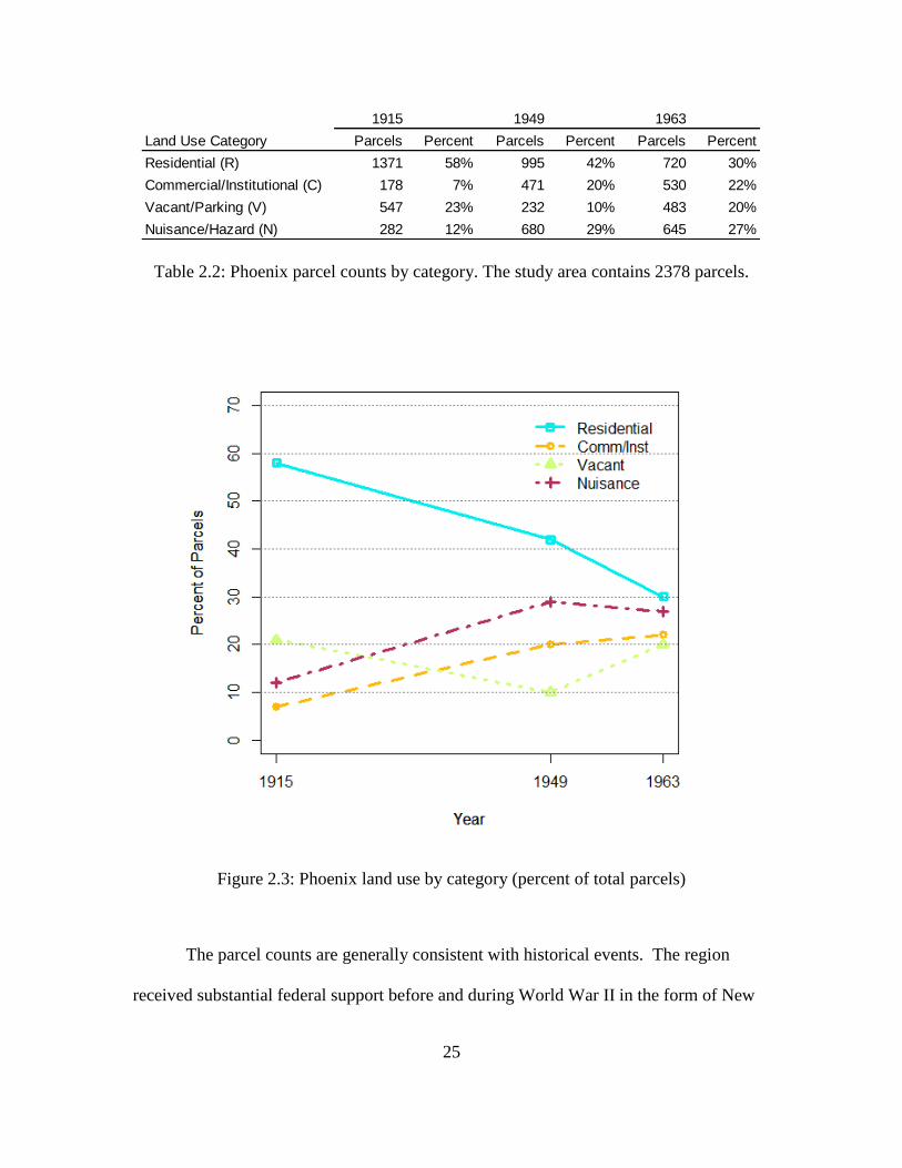
2.3.1 Quantity Disagreement: Phoenix Parcel Counts
Several trends are observed from simply counting parcels. Both
commercial/institutional and nuisance parcel counts increased substantially (nearly
tripling) by 1949 and remained relatively constant until 1963 (Table 2.2). The number of
vacant parcels decreased substantially by 1949, then more than doubled. A steep and
constant decrease occurred in residential land use over both periods. Interestingly, by
1963, parcel land use was almost evenly divided amongst the four classes (Figure 2.3).
25
Table 2.2: Phoenix parcel counts by category. The study area contains 2378 parcels.
Figure 2.3: Phoenix land use by category (percent of total parcels)
The parcel counts are generally consistent with historical events. The region
received substantial federal support before and during World War II in the form of New
1915 1949 1963
Land Use Category Parcels Percent Parcels Percent Parcels Percent
Residential (R) 1371 58% 995 42% 720 30%
Commercial/Institutional (C) 178 7% 471 20% 530 22%
Vacant/Parking (V) 547 23% 232 10% 483 20%
Nuisance/Hazard (N) 282 12% 680 29% 645 27%
26
Deal projects, so much that Del Webb, the region’s leading construction magnate,
remarked, “Construction is no longer a private enterprise, but rather a subsidiary of the
federal government” (Luckingham 1989). The decrease in vacancy and the increase in
commercial and nuisance (mostly industrial) parcels reflect the overall growth in
Phoenix’s early period. Downtown residential declines are expected, and are likely
reflective of the continual trend of affluent whites moving north, both within Phoenix and
to newer suburbs (Gober 2006). By 1963, commercial and nuisance uses retained a
similar proportion of parcels from the previous period, while a distinct change occurred
as residential counts declined and the number of vacant parcels more than doubled. Thus,
we see evidence of the emptying of the downtown area; however, the main loss of built
parcels appears to be residential and not commercial. Even though retail/commercial
parcels are combined with institutional land uses in our analysis, this appears to
contradict the assumption that retail decline and the construction of far-flung shopping
malls were the driving factor in the downtown’s decline.
2.3.2 Quantity Disagreement: Land Use Transition Analysis
Land use transition matrices for the frontier boom period and the postwar boom
period can be found in Table 2.3. All use types except vacant are more likely to stay the
same than to transition, which is expected as this category represents either a lack of land
use or, in the case of surface parking, the lack of substantial built investment in its use.
Given a null hypothesis of land use persistence, off-diagonal transition types should
occur significantly less frequently than the expected value based on population. Any
deviation from this pattern is noteworthy and is indicated by pseudo-significance values
other than 1.000, which show that in the 9999 permutations run, there were at least some
27
instances where that transition type occurred more frequently than expected by random
chance.
Table 2.3: Transition matrices showing change in land use category, expected values, and
simulated significance p-values.
In the frontier boom period, the vacant-to-commercial (p = 0.9995) and vacant-to-
nuisance (p = 0.0094) transitions were nearly as high as or higher than predicted by their
raw counts, indicating an expansion of business and industrial activity into previously
undeveloped land. Nuisance-to-commercial (p = 0.3340) and nuisance-to-vacant (p =
0.9594) transitions also occurred with high frequency. In the postwar boom period,
1949 Parcel Land Use 1963 Parcel Land Use
1915 Parcel LU R C V N 1949 Parcel LU R C V N
Residential (R) 797 180 95 299 Residential (R) 661 78 189 67
58% 13% 7% 22% 66% 8% 19% 7%
[574] [272] [134] [392] [301] [222] [202] [270]
0.0001 1.0000 1.0000 1.0000 0.0001 1.0000 0.9197* 1.0000
Comm/Inst (C) 7 150 5 16 Comm/Inst (C) 25 330 57 59
4% 84% 3% 9% 5% 70% 12% 13%
[74] [35] [17] [51] [143] [105] [96] [128]
1.0000 0.0001 1.0000 1.0000 1.0000 0.0001 0.0001 1.0000
Vac/Park (V) 174 82 112 179 Vac/Park (V) 23 34 115 60
32% 15% 20% 33% 10% 15% 50% 26%
[229] [108] [53] [156] [70] [52] [47] [63]
1.0000 0.9995* 0.0001 0.0094* 0.0001 0.9989* 0.0001 0.6926*
Nuis/Hazard (N) 17 59 20 186 Nuis/Hazard (N) 11 88 122 459
6% 21% 7% 66% 2% 13% 18% 68%
[118] [56] [28] [81] [206] [152] [138] [184]
1.0000 0.3340* 0.9594* 0.0001 1.0000 1.0000 0.9713* 0.0001
N ij Number of parcels (Bold)
P ij Row standardized percent (Italics)
E ij [Expected Value] (brackets)
p-value (* if different from expectation of persistence)
28
residential-to-vacant (p = 0.9197) and nuisance-to-vacant (p = 0.9713) transitions
approached the population-predicted values, corroborating the earlier result of residential
exodus from downtown, but now suggesting that industry may have been leaving too.
However, vacant-to-commercial (p = 0.9989) and vacant-to-nuisance (p = 0.6926)
transitions were not substantially lower than population-predicted values, indicating that
the trend toward vacancy was not universal.
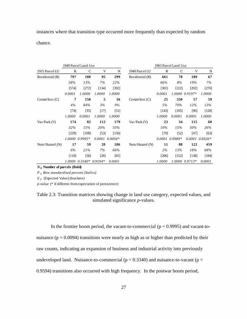
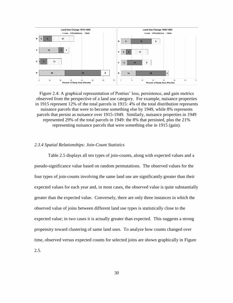
2.3.3 Allocation Disagreement: Pontius Transition Scores
Results for Pontius’ metrics can be found numerically in Table 2.4 and
graphically in Figure 2.4. In the frontier boom period, the measures for persistence, loss,
gain, swap, and total change are relatively straightforward and are expressed as a
proportion of the total distribution. The aforementioned nuisance gains are offset with
slight loss, while vacancy losses are offset with slight gain. Commercial/institutional
gains are substantial and are accompanied by virtually no losses. Residential losses,
while substantial, are slightly offset with residential gains (0.08). The postwar boom
period shows a much more dynamic picture of change, especially because the data cover
a much shorter time period (fourteen years as opposed to thirty-four). Simple counts of
land use types suggest that the vacancy increase in this period was due to the decrease in
residential use, and the scores in Table 2.4 confirm that residential loss was hardly
accompanied by residential gains elsewhere. Evidence of commercial exodus is now
found: commercial/institutional, despite a slight net gain, shows a high amount of swap
and total change. This likely reflects a decrease in commercial use and an increase in
government presence downtown, which was known to have happened during this time.
Nuisance parcels exhibit a similar pattern of high swap, indicating that nuisance
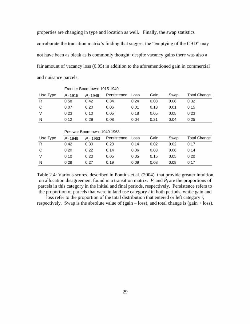
29
properties are changing in type and location as well. Finally, the swap statistics
corroborate the transition matrix’s finding that suggest the “emptying of the CBD” may
not have been as bleak as is commonly thought: despite vacancy gains there was also a
fair amount of vacancy loss (0.05) in addition to the aforementioned gain in commercial
and nuisance parcels.
Table 2.4: Various scores, described in Pontius et al. (2004) that provide greater intuition
on allocation disagreement found in a transition matrix. Pi and Pj are the proportions of
parcels in this category in the initial and final periods, respectively. Persistence refers to
the proportion of parcels that were in land use category i in both periods, while gain and
loss refer to the proportion of the total distribution that entered or left category i,
respectively. Swap is the absolute value of (gain – loss), and total change is (gain + loss).
Use Type P i 1915 P j 1949 Persistence Loss Gain Swap Total Change
R 0.58 0.42 0.34 0.24 0.08 0.08 0.32
C 0.07 0.20 0.06 0.01 0.13 0.01 0.15
V 0.23 0.10 0.05 0.18 0.05 0.05 0.23
N 0.12 0.29 0.08 0.04 0.21 0.04 0.25
Use Type P i 1949 P j 1963 Persistence Loss Gain Swap Total Change
R 0.42 0.30 0.28 0.14 0.02 0.02 0.17
C 0.20 0.22 0.14 0.06 0.08 0.06 0.14
V 0.10 0.20 0.05 0.05 0.15 0.05 0.20
N 0.29 0.27 0.19 0.09 0.08 0.08 0.17
Frontier Boomtown: 1915-1949
Postwar Boomtown: 1949-1963
30
Figure 2.4: A graphical representation of Pontius’ loss, persistence, and gain metrics
observed from the perspective of a land use category. For example, nuisance properties
in 1915 represent 12% of the total parcels in 1915: 4% of the total distribution represents
nuisance parcels that were to become something else by 1949, while 8% represents
parcels that persist as nuisance over 1915-1949. Similarly, nuisance properties in 1949
represented 29% of the total parcels in 1949: the 8% that persisted, plus the 21%
representing nuisance parcels that were something else in 1915 (gain).
2.3.4 Spatial Relationships: Join-Count Statistics
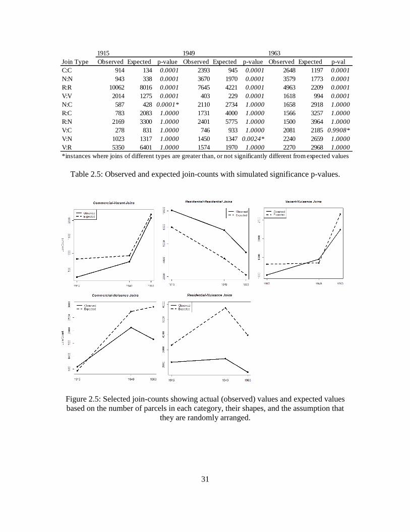
Table 2.5 displays all ten types of join-counts, along with expected values and a
pseudo-significance value based on random permutations. The observed values for the
four types of join-counts involving the same land use are significantly greater than their
expected values for each year and, in most cases, the observed value is quite substantially
greater than the expected value. Conversely, there are only three instances in which the
observed value of joins between different land use types is statistically close to the
expected value; in two cases it is actually greater than expected. This suggests a strong
propensity toward clustering of same land uses. To analyze how counts changed over
time, observed versus expected counts for selected joins are shown graphically in Figure
2.5.
31
Table 2.5: Observed and expected join-counts with simulated significance p-values.
Figure 2.5: Selected join-counts showing actual (observed) values and expected values
based on the number of parcels in each category, their shapes, and the assumption that
they are randomly arranged.
Join Type Observed Expected p-value Observed Expected p-value Observed Expected p-val
C:C 914 134 0.0001 2393 945 0.0001 2648 1197 0.0001
N:N 943 338 0.0001 3670 1970 0.0001 3579 1773 0.0001
R:R 10062 8016 0.0001 7645 4221 0.0001 4963 2209 0.0001
V:V 2014 1275 0.0001 403 229 0.0001 1618 994 0.0001
N:C 587 428 0.0001* 2110 2734 1.0000 1658 2918 1.0000
R:C 783 2083 1.0000 1731 4000 1.0000 1566 3257 1.0000
R:N 2169 3300 1.0000 2401 5775 1.0000 1500 3964 1.0000
V:C 278 831 1.0000 746 933 1.0000 2081 2185 0.9908*
V:N 1023 1317 1.0000 1450 1347 0.0024* 2240 2659 1.0000
V:R 5350 6401 1.0000 1574 1970 1.0000 2270 2968 1.0000
*instances where joins of different types are greater than, or not significantly different from expected values
1915 1949 1963
32
In order to examine the character of the commercial outflow from downtown, we
observe commercial-to-vacant joins. A low starting value, combined with far higher than
expected commercial-commercial joins in 1915 indicates a tightly spaced commercial
district. By 1949, the observed and expected values of commercial-vacant joins began to
converge and by 1963 the observed count was only slightly below expectations – so
much that there is a slight statistical chance (p = 0.9908) that commercial/institutional
parcels are as likely to be within 200 feet of vacant parcels or surface parking as their raw
counts suggest.
The residential-residential join-count is far above the expected value in all cases
and is not statistically significant. Despite fewer residential parcels, the residential-
residential join-count continually increases relative to the expected value, indicating
residential homogenization consistent with the story of wealthier, white, non-Hispanic
residences continually pushing north from the CBD. Thus, we find evidence of an urban
landscape where commercial parcels are found in close proximity to recently vacated
former residences, which is consistent with the results from the transition matrices.
Additionally, though the idea of downtown decay might be consistent with
incompatible land uses – especially with weak zoning regulations – there is a noteworthy
change in the joins related to nuisance properties. Commercial-nuisance joins actually
begin above the expected value in 1915 but are significantly below it in 1949, indicating
that these uses – once exhibiting a high propensity toward clustering – are sorting out
even though this relationship is substantially more common. Then, despite an
expectation of a slight increase, they drop precipitously during the postwar period.
Residential-nuisance joins are not significantly similar to expected values though their
33
change over time is interesting. Despite a large expected increase, they stay relatively
stable during the frontier boom period, followed by a continued (but expected) drop in
the postwar period. In both cases, we see a continual decrease in the instance of higher
order uses existing in close proximity to nuisance parcels. It would appear as though
nuisance properties are less likely to be a nuisance to their neighbors. Interestingly, the
residential sorting away from nuisance was more pronounced in the frontier boom period
while the commercial sorting was greater in the postwar period, indicating that the
residential move northward and outward preceded the commercial changes downtown.
Finally, vacant-nuisance joins are also indicative of somewhat haphazard growth in the
frontier period followed by postwar sorting: lower than expected in 1915, they are
significantly greater than expected in 1949, and drop below again in 1963.
2.3.5 Spatial Relationships: Spatial Markov Approach
The row-standardized transition matrices for both periods are shown as 4 x 4 x 4
matrices in Table 2.6. A byproduct of our categorical distribution is that the parcels
represent actual land use types and are not arbitrary thresholds determined for this
analysis, such as quartiles of a continuous income distribution. Therefore, some of our
spatial lag designations can be sparsely populated, resulting in several lagged transition
types that are undergone by only one or no parcels. In these instances, care must be taken
not to overstate the importance of one’s inferences.
34
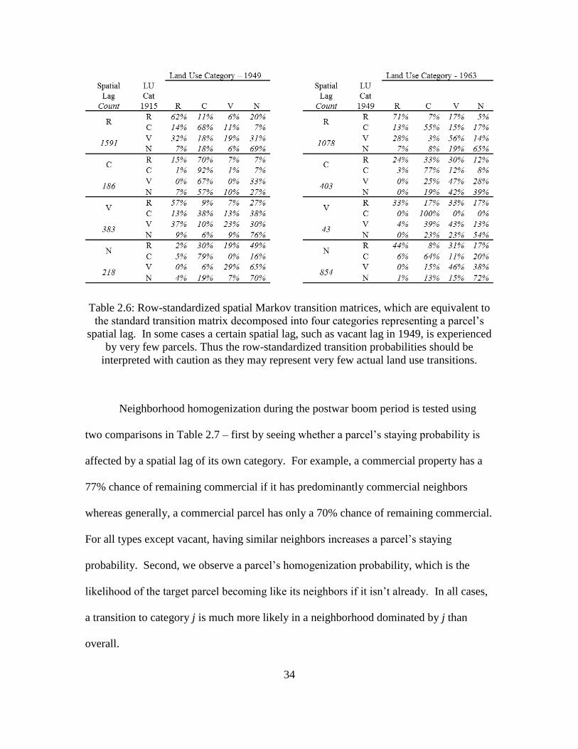
Table 2.6: Row-standardized spatial Markov transition matrices, which are equivalent to
the standard transition matrix decomposed into four categories representing a parcel’s
spatial lag. In some cases a certain spatial lag, such as vacant lag in 1949, is experienced
by very few parcels. Thus the row-standardized transition probabilities should be
interpreted with caution as they may represent very few actual land use transitions.
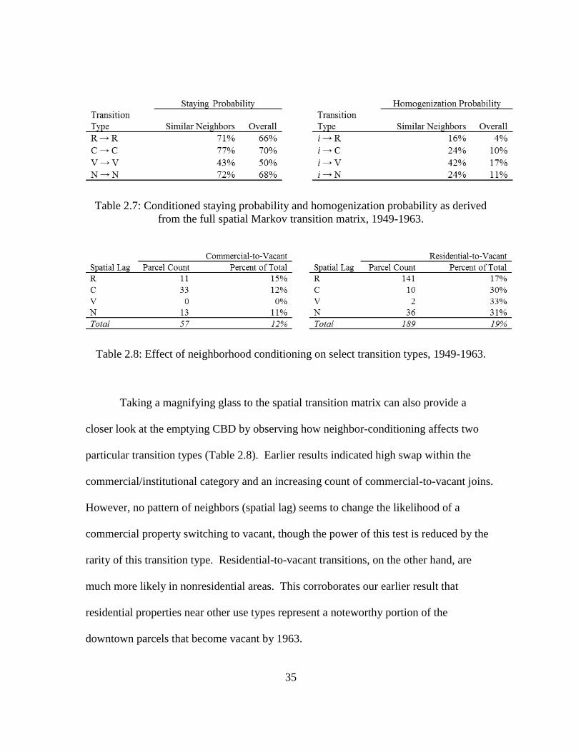
Neighborhood homogenization during the postwar boom period is tested using
two comparisons in Table 2.7 – first by seeing whether a parcel’s staying probability is
affected by a spatial lag of its own category. For example, a commercial property has a
77% chance of remaining commercial if it has predominantly commercial neighbors
whereas generally, a commercial parcel has only a 70% chance of remaining commercial.
For all types except vacant, having similar neighbors increases a parcel’s staying
probability. Second, we observe a parcel’s homogenization probability, which is the
likelihood of the target parcel becoming like its neighbors if it isn’t already. In all cases,
a transition to category j is much more likely in a neighborhood dominated by j than
overall.
35
Table 2.7: Conditioned staying probability and homogenization probability as derived
from the full spatial Markov transition matrix, 1949-1963.
Table 2.8: Effect of neighborhood conditioning on select transition types, 1949-1963.
Taking a magnifying glass to the spatial transition matrix can also provide a
closer look at the emptying CBD by observing how neighbor-conditioning affects two
particular transition types (Table 2.8). Earlier results indicated high swap within the
commercial/institutional category and an increasing count of commercial-to-vacant joins.
However, no pattern of neighbors (spatial lag) seems to change the likelihood of a
commercial property switching to vacant, though the power of this test is reduced by the
rarity of this transition type. Residential-to-vacant transitions, on the other hand, are
much more likely in nonresidential areas. This corroborates our earlier result that
residential properties near other use types represent a noteworthy portion of the
downtown parcels that become vacant by 1963.
36
2.4 Discussions
The previous section presented the results of each individual method. In this
section we consider all results in light of our three research questions: (1) what landscape
results from the changing composition of the downtown that accompanied postwar
suburban dominance, (2) to what extent is land use homogenization or incompatibility
observed, and (3) how do nuisances and hazards become distributed as the city changes?
First, the perceived emptying out of the CBD from 1949-1963 was more complex
than just a retail exodus. Raw numbers suggest a shift from residential to vacant parcels.
Pontius’ metrics show high swap within the commercial/institutional category, suggesting
that our aggregation of the two types may hide retail loss behind an increase in
government presence downtown. Nonetheless, they indicate that
commercial/institutional parcels are changing location, though not decreasing in total
quantity. Join-counts show an increase in the likelihood of a commercial and vacant
property being situated near each other. The spatial Markov matrix indicates this is likely
related to residential exodus: residential properties are more likely to vacate if in
commercial/institutional neighborhoods, leaving commercial parcels next to vacant ones.
This creates a street-level atmosphere of languishing retail, government buildings, and
other commercial/institutional properties which continues in Phoenix’s downtown to this
day.
The emptying of downtown can be seen very clearly on the map in Figure 2.2: a
ring of vacancy seems to appear by 1963, surrounding the center of downtown in areas
that look to have been a mix of uses in 1949. Our metrics indicate that, in terms of actual
parcels, this decline was more directly tied to residential exodus than overall commercial
37
decline, though these processes certainly operate hand-in-hand. This demonstrates the
validity of Sternlieb (1963)’s understanding of positive feedbacks, wherein residential
outflow moved middle-class customers away from downtown retail, which languished
itself and eventually moved too. Furthermore, we see some evidence that this emptying
out did not represent a wholesale hollowing out of economic activity which befell some
older industrial cities like Detroit. Vacant-to-commercial and vacant-to-nuisance
transitions continued to occur while Pontius metrics actually show some vacancy loss in
the CBD.
Second, we see several indications of land use homogenization and a decline in
the incidence of undesirable incompatibility. Most clearly, spatial Markov matrices
indicate strong homogenization pressure during the postwar period, wherein a parcel is
more likely to remain in the same category if it is near parcels of the same type and far
more likely to change to the same land use of its neighbors if it is dissimilar. Join-counts
and spatial Markov matrices suggest the decrease in residential parcels in downtown
Phoenix is not characterized by vacant patches within residential neighborhoods. Instead,
it reflects large-scale residential exodus. This is consistent with the commonly held
narrative of white, non-Hispanic, and wealthier residences continually moving north
within Phoenix and to the newly built post-war suburbs. Again, this can be seen on the
map in Figure 2.2: by 1963 there appear to be far fewer residential parcels downtown and
those that remain are heavily concentrated north of Van Buren Street.
Finally, we find evidence of a continual decrease in residential and commercial
uses existing in close proximity to nuisance parcels in the study area. While industrial
activity has always concentrated around the railroads in the southern portion of
38
downtown, nuisance/hazard parcels become increasingly concentrated in these areas and
other uses generally move elsewhere (which again can be seen in the map in Figure 2.2).
This change is apparent in general terms as well: by 1949 nuisance parcels are
decreasingly found in close proximity to residential areas and by 1963 their likelihood of
being near commercial parcels drops sharply too. This provides evidence that Phoenix’s
downtown is increasingly ordered in terms of Euclidian land use categories despite
concerns that rapid change, poor zoning enforcement, and capital outflow would result in
incompatibility.
2.5 Conclusions
The goal of this chapter is to use parcel-level land use data from Phoenix to link
land-use change processes from historical narratives to observed changes in urban
morphology by drawing on quantitative traditions in urban growth modeling, ecological
modeling, and spatial analysis. This approach helps us understand the connection
between urban landscapes and the micro-level processes that lead to their creation. The
insights gained are critical to pushing forward planning policies that recognize the role of
parcel-level land use decision making and could be utilized by planners and New
Urbanist scholars to empirically understand historical processes that led to the
neighborhood and landscape patterns that they are either trying to avoid or recreate.
Examining parcel-level change can lead to some emergent insights that may not be
perceived with a broader narrative approach such as the role played by land use swapping
within the commercial/institutional category or the importance of the residential exodus
in downtown’s commercial decline. Understanding changes in the way parcels are
allocated in a city is an important component of urban revitalization and directly impacts
39
walkability, land use complementarity, and ultimately urban sustainability. This
examination and approach provide a step toward a more nuanced understanding of
urbanization processes and patterns within an exponentially growing Sunbelt city.
The postwar downtown decline is emblematic of broader regional changes in
Phoenix and is a key part in the story of automobile dependence and suburbanization.
Unpacking the observed land use pattern suggests that landowners’ parcel-level decision-
making resulted in a pattern of commercial areas interspersed with vacancy, which helps
to explain modern downtown Phoenix’s swaths of vacant land and surface parking—
legacies of a postwar downtown decline. While the extent of residential and nuisance
properties’ propensity toward sorting may have been unexpected given the CBD’s
decline, this study provides quantitative support for the narratives about northward
residential movement and industrial concentration south of downtown.
Ongoing work (see Chapter 3) aims to link drivers of land-use change to land
cover data, thereby extending the utility of a parcel-level analysis to more recent concerns
about urban micro-climates and regional water use. A further approach that integrates
similar space-time analysis with econometrics could model the impact of zoning policies
or observe the effect of urban development subsidies on urban morphology, linking
policy and land use outcomes directly (see Chapter 4). Historical legacies continue to
determine the future trajectory of urban areas throughout the U.S. This quantitative,
historical analysis of one city emblematic of automobile sprawl has improved the link
between drivers of land-use change and urban morphology by showing how historic
developments have transformed the urban landscape into what it is today.
40
CHAPTER 3
BEYOND FRAGMENTATION AT THE FRINGE
3.1 Introduction
Patterns of human settlement are changing rapidly around the world as the global
population becomes increasingly urban. In addition, economic and social changes affect
the pattern of land use and land cover within cities, altering the structure and form of
urban environments. These changes in spatial structure in turn transform ecological
functions, such as hydrological systems and biogeochemistry (Grimm et al. 2008).
Changes in land cover and ecological process have far reaching impacts for ecosystem
services, which in turn shape various social and economic outcomes (Tratalos et al. 2007,
Bolund and Hunhammar 1999). As urbanization continues and urban spatial pattern
evolves, research is needed to inform planning and management of urban areas,
addressing the causes and impacts of different urbanization patterns (Longley and Mesev
2000, Klosterman 1999), which are heavily impacted by policy (Newburn and Berck
2006, Carruthers 2003).
Urban form and patterns of urban growth have long been of interest to
geographers. This topic has been widely explored in relation to socioeconomic activities
(see, e.g., Knox 1991), but more recently scholars have become interested in
environmental implications: namely, how different spatial patterns in cities may impact
ecosystem processes with implications for ecosystem services and adaptation to
environmental change (e.g., Alberti 2005, Alberti and Marzluff 2004; Turner et al.,
2013). Concerns for both socioeconomic and biophysical implications of urban spatial
pattern are often aired in conjunction with critiques over urban sprawl. Definitions of
41
urban sprawl vary, but the term generally refers to the excessive spatial growth of cities
(Brueckner 2000), which is characterized by low-density development and automobile-
dominated infrastructure and lifestyles (Bruegmann 2005). Considering the variety of
phenomena encompassed, Ewing, Pendall and Chen (2002) suggest three specific spatial
dimensions of sprawl: low-density population, new development on the periphery
without a clear activity center, and widely separated built structures.
Additionally, the form and style of agglomeration is highly dependent on place
and historical context (Bruegmann 2005). Urban spatial structure is heavily path-
dependent (Arthur 1988), continuously characterized by the infrastructure and planning
of past periods of development. The way a neighborhood looks today is largely reflective
of the era during which it was built, “locking in” the effect of short-term housing booms,
the principal economic activities of the time, and the dominant communication and
transportation technology (Adams 1970, Anas, Arnott and Small 1998). Given these
legacy effects of urbanization, understanding the characteristics of historical time periods
during which growth occurred can inform the understanding of present-day landscape
variation.
Research analyzing the detailed characteristics of patterns of sprawl has been
supported by the increasing availability of spatial data and the development of new
methods of spatial analysis. Whereas earlier geographic analyses were often limited by
data availability, recent studies have benefited from the proliferation of earth observing
(EO) sensors to examine specific changes in urban landscapes, and to evaluate theories of
urban development (e.g., Dietzel et al. 2005, Taubenböck et al. 2014). EO methods
provide the ability to examine regional, continental, and even global scales. At regional
42
scales, sprawl studies have employed EO data to examine agglomeration around urban
cores (Taubenböck et al. 2014, Dietzel et al. 2005) and to facilitate comparison between
urban areas (Burchfield et al. 2006, Schneider and Woodcock 2008), examining changes
in the extent of built-up areas or even changes in vertical structure across different cities
(Frolking et al. 2013). These comparisons of urbanization around the world reveal
distinct patterns of growth, suggesting that growth trajectories vary across cities
(Schneider and Woodcock 2008). To facilitate such comparison and to capture the more
nuanced characteristics of urbanization, Seto and Fragkias (2005) call for a diverse set of
quantitative measurements that describe various facets of urban growth and that help to
infer the underlying processes that drive observed urban forms. Similarly, Siedentop and
Fina (2010) suggest that a multi-indicator approach should be used to identify three
aspects of sprawl: urban density, pattern, and composition.
In order to characterize such aspects of urban spatial pattern, an increasing
number of urban studies have employed an array of spatial metrics common in landscape
ecology (Turner 1989). Spatial metrics provide measures of landscape pattern derived
from the analysis of thematic-categorical maps, which first segment the observed
landscape into patches of adjacent pixels of the same class and then use this information
to quantify landscape patterns. Spatial metrics commonly provide descriptive measures
of the spatial characteristics of individual patches, all patches in a given class, or all
patches in the landscape. Various metrics have been developed (Turner et al. 1989, Li
and Reynolds 1993) and implemented in different software packages, most notably
FRAGSTATS (McGarigal and Marks 1994). Ecologists have long employed these tools
because changes in the shape, size, prevalence, and connectivity of different land cover
43
patches, as well as the positions of these land covers relative to each other, can have
significant impacts on various ecological processes (Turner 1989, Turner, Gardner and
O'Neill 2001). Studies of sprawl commonly incorporate these metrics, but often only
identify two thematic classes that distinguish between “developed” and “undeveloped”
patches. Nonetheless, EO datasets can support more complex classification schemes,
which can be useful to characterize specific features of certain regions (for example,
identifying structure types within informal settlements in the developing world, see
Kuffer and Barros 2011, Banzhaf and Hofer 2008), but these are partially dependent on
the resolution of the EO data.
In recent years, numerous studies have applied landscape metrics to the study of
urban morphology (e.g. Wu and Webster 2000, York and Munroe 2010), most commonly
employing moderate resolution data, such as Landsat and the National Land Cover
Dataset (NLCD), which consist of 30m x 30m pixels. For example, York et al. (2011a)
and Zhang et al. (2013) used Landsat-derived data to estimate metrics of fragmentation in
several rapidly growing US cities and demonstrated that fragmentation typically increases
with distance from the city center. McDonnell and Hahs (2008) review 300 papers that
rely on the variation of urban intensity along an urban-rural gradient in order to
understand differences in ecosystem processes, but little of this research has empirically
assessed differences in detailed spatial patterns of land cover (beyond general categories
of land use) or small scale habitats.
Moderate resolution analyses offer important information on regional scale
change, but increasingly complex use of urban space necessitates a scale-sensitive,
micro-level approach (Irwin, Jayaprakash and Munroe 2009) – a perspective shared by
44
ecologists (Wu and Loucks 1995, Pickett et al. 1997). The moderate resolution imagery
relied upon for most prior studies has proven useful for tracking the expansion of urban
areas, but is ill-suited for capturing the fine details that characterize urban landscapes
(Theobald 2001, Herold, Couclelis and Clarke 2005, Irwin and Bockstael 2007). For
example, Burchfield et al. (2006), develop an index of sprawl using NLCD data and find
that, across the entire US, the extent of scatteredness in urban areas was essentially
unchanged from 1976 to 1992. Irwin and Bockstael (2007) challenge their conclusions,
augmenting NLCD data with land use records in Maryland to demonstrate that
fragmentation (using landscape metrics) is not static over time, does vary across an
urban-rural gradient, and requires a finer resolution approach. Recognizing this need,
some studies have begun to use landscape metrics to analyze finer resolution data to
identify and characterize specific components of urban form. Taubenböck and Kraff
(2013) used spatial metrics of high resolution data to identify the physical properties of
slums in Mumbai using Quickbird imagery (0.6m resolution). Kuffer and Barros (2011)
used Quickbird and Ikonos (4m resolution) in Dar es Salaam and Delhi to identify
unplanned areas in cities. Similarly, Banzhaf and Hofer (2008) used object-based
methods on aerial photographs to identify specific types of urban structures. In
combination, these examples illustrate the potential application of high-resolution
datasets and pattern analysis techniques to improved characterization of urban landscape
features.
This paper analyzes fine-grained aspects of sub-metropolitan spatial pattern in
Phoenix, Arizona based on when an area within the city was developed, relying on the
path-dependent nature of cities to understand variation in present-day patterns of land
45
cover. Urban morphology is largely the product of historical development trends, while
the durability of built capital means that the environmental consequences of development
will persist for several decades after the process that led to their construction has played
out. In particular, Boone et al. (2012) argue that the timing of development is crucial for
urban ecosystem structure and function. Put simply, different areas within a city are
expected to have different landscape characteristics based on when they were built. This
study adds to the literature above because it 1) uses higher resolution spatial data, 2) uses
high thematic resolution (i.e., beyond developed/undeveloped), and 3) considers variation
in spatial pattern by historical development periods rather than by intrametropolitan
location. This study uses one-meter resolution NAIP (National Agriculture Imagery
Program) images of Phoenix, Arizona from 2010, which has the ability to identify
variation within parcels of land – including, for example, individual trees, sidewalks, and
patches of lawn. Spatial metrics are used to identify four characteristics of land cover
relevant to urban sprawl: area and density, fragmentation, shape complexity, and
diversity. These metrics are analyzed across 946 sub-metropolitan units in Phoenix
(census block groups) based on the time period in which they were developed in order to
understand how present-day urban spatial pattern varies based on when areas of the city
became developed.
3.2 Material and Methods
3.2.1 Study Area
Phoenix’s urban history did not begin in earnest until the start of the twentieth
century. The city’s 1915 boundaries, generally considered to be the “original townsite”
(York et al., 2014) encompass 10.4 square kilometers, while its 2012 boundaries include
46
2,079 square kilometers. Residential land use dominates the city in terms of land area,
comprising 69% of the built-up area in its historic core in 1915 and 62% of the built-up
area in 2012 (Kane et al. 2014c). The urban (developed) extent of the entire metropolitan
area increased similarly from 48 square kilometers in 1934 to 2,537 square kilometers in
2010 (Knowles-Yanez et al. 1999 and authors' calculations).
Early growth in Phoenix followed a relatively concentric pattern extending
outward from the Central Business District (CBD), facilitated by the limited presence of
existing manmade features and the fact that automobile transportation was adopted fairly
early in the city’s history (VanderMeer 2002). This pattern began to change in the early
1960s when the CBD ceased to be a major draw and growth became more polycentric
and dispersed (Kane et al. 2014b). Development styles contrast dramatically across time
periods, in Phoenix and in general (Judd and Swanstrom 2008, Gober 2006). Early
homes and businesses of the 1920s, localized near downtown, were largely built in the
same manner as in older cities. Mass-produced single-story tract homes characterized
residential construction following World War II, while gated and master-planned
communities became popular beginning in the 1970s. During the latter period, large
shopping malls and office parks supplanted older commercial space in Phoenix’s CBD.
Discussion of more recent changes typically focuses on fringe development, with the real
estate boom that began in the late 1990s taking place most prominently farther from the
city center (Gober and Burns 2002). This happened in “boomburbs” such as Chandler
and Gilbert but also in the far northern and southern parts of the City of Phoenix.
Atkinson-Palombo (2010) finds that growth during the early 2000s was more varied than
the prior decade, with denser, multifamily housing near the urban fringe augmenting
47
single-family development there. Additionally, conversion of former agricultural land
ground to a halt during the 2006-2008 recession (Kane et al. 2014c).
3.2.2 Delineating Historical Periods
The purpose of this study is to investigate how spatial indicators of urban sprawl
vary across areas within a city based on the time period during which present-day
structures were built. While a city-wide indicator of sprawl may be interesting in a cross-
site context, our goal is to capture sub-metropolitan variation in sprawl indicators,
following the idea within urban design that geographic pattern informs a sense of place
and drives the experiences of individuals (see, e.g., Talen 2011), and that environmental
implications of development such as the urban heat island are often localized (see, e.g.,
Connors, Galletti and Chow 2012). Furthermore, the surroundings of an individual are
not confined to a single land parcel, but also include the streets, public spaces, and other
land uses nearby. Thus it is necessary to define an appropriate areal unit at which to
analyze sprawl.
Prior studies such as Shrestha et al. (2012) and Zhang et al. (2013) use a grid or a
rectangular moving window. Instead, we chose to use US Census Block Groups because
they are intentionally delineated by the Census Bureau such that they contain between
600 and 3,000 people. While a block group certainly does not define an actual
neighborhood, this characteristic ensures that each block group represents some
functional urban space. Furthermore, block groups are the closest census aggregation
unit to the optimal moving window size suggested by Zhang et al. (2013). The City of
Phoenix is comprised of 977 block groups. Excluding 19 unusually large (larger than
11.5km2) block groups which represented large conservation areas or unoccupied desert,
48
block groups in this study range in size from 0.08km2 to 11.3km
2, with a mean of
1.02km2
and standard deviation of 1.20km2
(N = 958). Our study calculates landscape
metrics for all block groups and does not rely on random sampling.
Reliable data on buildings and structures for the city of Phoenix are available
from the Maricopa County Assessor’s Office and were cross-checked with the Maricopa
Association of Governments, a regional planning body. These data record the
construction year of the buildings on each land parcel as of 2012. In order to identify the
historical time period during which development in a block group began to resemble its
present-day form, we describe each block group using the decade by which half of the
present-day structures had been built. While some buildings in Phoenix date back to the
1880s, the oldest block group using this classification technique is actually from the
1920s (Figure 3.1). However, only one block group is dominated by 1920s construction,
two are dominated by 2010s construction, and nine block groups date principally from
the 1930s. In contrast, defining historical zones by the age of the oldest building in an
area, or by the time period during which the most construction occurred is less consistent
with the path-dependent nature of development. Our goal is to identify when a sub-
metropolitan area became “substantially developed” relative to its present-day land cover
characteristics.
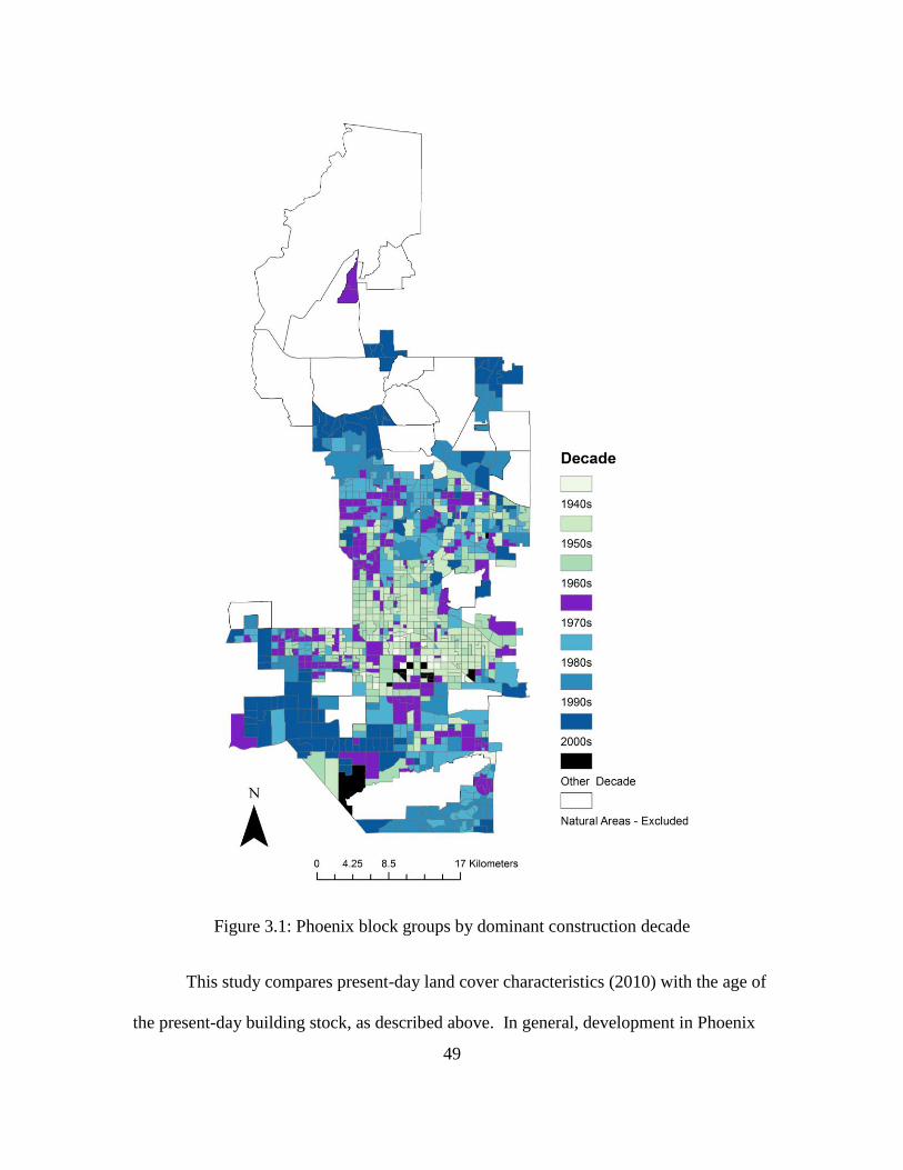
49
Figure 3.1: Phoenix block groups by dominant construction decade
This study compares present-day land cover characteristics (2010) with the age of
the present-day building stock, as described above. In general, development in Phoenix
50
is continually characterized by a desire for new construction in new areas (Gober 2006).
Infill development is comparatively rare: buildings are not often knocked down, which
makes this method of using public records from 2012 to identify historical zones a
reasonably accurate indicator of when an area was originally developed.
3.2.3 Image Classification
The satellite images were classified using object-based image analysis (OBIA)
and classification methods. OBIA methods are increasingly favored for the classification
of high-resolution images because they can take advantage of the spatial and contextual
information present at finer scales (Benz et al. 2004, Blaschke 2010). OBIA methods
have two stages: segmentation and classification. Image segmentation involves grouping
adjacent pixels with similar values into objects (Baatz and Schape 2000). Once formed,
objects may then be assigned various values based on spectral and spatial properties
calculated from all of the encapsulated pixels (e.g. averaging the reflectance of all pixels
in the object). Objects are then assigned to discrete land cover classes using decision-
based rule sets or automated algorithms. A set of decision-based rules is then used to
classify the objects. Seven land cover classes were extracted from the classified NAIP
image: buildings, roads, trees, grass, soil, shrubs, and croplands. After the classification,
the results were inspected and obvious errors were manually corrected. Using this
approach, we were able to achieve 91.86% accuracy (Li et al. 2014).
The decision to use these seven land cover classes (buildings, roads, trees, grass,
soil, shrubs, and cropland) is based on changing development patterns in Phoenix and
previous studies (e.g. Myint et al. 2013). These land cover classes were chosen to capture
the heterogeneity of urban parcels in Phoenix, particularly the variation in residential
51
landscaping. This finer thematic resolution, identifying land covers beyond the
urbanized-nonurbanized dichotomy, provides the ability to examine detailed patterns in
urban form and development. The land cover scheme includes some land covers that are
natural to the American Southwest, such as desert soil and shrubs, but these features were
largely replaced by turf lawns and non-native vegetation during earlier development
periods (particularly in the 1960’s and 1970’s). New trends in development, however,
have encouraged so-called xeric landscaping, which changes the land cover in residential
areas from what would have been turf grass and trees to something that might mimic
natural desert, such as soils. Because cropland and shrub classes represented only a very
small proportion of the total land area within the Phoenix city limits, we excluded them
from our subsequent statistical analyses.
3.2.4 Subset Images
Analysis is conducted at the block group level to provide an approximation of
neighborhood areas, and in order to facilitate future comparison to census data. Using an
automated process in a Python code 958 image subsets were extracted each conforming
to the boundary of one census block group. In other words, using the boundaries of each
individual block group in the City of Phoenix, the classified image was clipped to create
958 separate images for analysis. To illustrate this process, Figure 3.2 shows a selection
of these subset land cover images for six different block groups from different historical
zones.
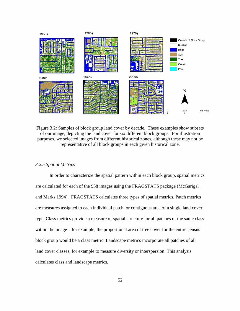
52
Figure 3.2: Samples of block group land cover by decade. These examples show subsets
of our image, depicting the land cover for six different block groups. For illustration
purposes, we selected images from different historical zones, although these may not be
representative of all block groups in each given historical zone.
3.2.5 Spatial Metrics
In order to characterize the spatial pattern within each block group, spatial metrics
are calculated for each of the 958 images using the FRAGSTATS package (McGarigal
and Marks 1994). FRAGSTATS calculates three types of spatial metrics. Patch metrics
are measures assigned to each individual patch, or contiguous area of a single land cover
type. Class metrics provide a measure of spatial structure for all patches of the same class
within the image – for example, the proportional area of tree cover for the entire census
block group would be a class metric. Landscape metrics incorporate all patches of all
land cover classes, for example to measure diversity or interspersion. This analysis
calculates class and landscape metrics.
53
Schneider and Woodcock (2008) identified four urban growth indicators: size of
built-up area and rate of change, density of built-up land, fragmentation, and population
density. Whereas they conducted an interurban analysis, this study is concerned with
intraurban characteristics and therefore modifies this framework to suit the higher spatial
and thematic resolution of our one-city analysis. Rather than looking at size and density
of built up areas, we consider the size and density of each land cover class because we are
concerned with variation within built-up areas. Similarly, we consider the fragmentation
of each land cover type rather than fragmentation of non-built up areas en masse.
Following Herold, Liu and Clark (2003), who use 4-meter Ikonos imagery to analyze
urban areas, we also investigate fractal dimension and contagion indices as measures of
shape complexity. Interspersion and diversity are considered because these metrics are
widely used to characterize fragmentation, particularly in studies of lower thematic
resolution examining encroachment on non-urban lands. In sum, the selected metrics
concern the 1) area and density of land covers 2) fragmentation/scatter, 3) shape
complexity, and 4) diversity. These characteristics were selected because of their
relevance to the broader definitions of urban sprawl, discussed above, and the specific
metrics were selected because of their use in prior studies, thus facilitating comparison.
The six landscape and five class metrics chosen are outlined in Table 3.1.
54
Table 3.1: Basic description of spatial metrics used
3.2.6 ANOVA
In order to analyze the differential impact of the timing of development on
present-day land cover, we used Analysis of Variance (ANOVA) to identify statistically
significant differences in spatial metrics between development periods. Tukey’s HSD
post-hoc test creates a confidence interval and significance value (p-value) for each pair
of decades, using block groups as the unit of analysis. Since very few block groups
became substantially developed (relative to their present-day form) prior to the 1940s or
55
since the 2000s, we compare decades from the 1940s until the 2000s. Thus the statistical
analysis is performed on a total of 946 block groups.
3.3 Results
Comparing the historical zones, the results reveal that more recently constructed
areas differ in several ways from their older counterparts. In general, many landscape and
class metrics appear to significantly vary based on the time periods during which areas
were developed, which have in turn shaped variation in Phoenix’s spatial structure. Many
metrics, however, remain consistent across the different historical zones. Below, we
discuss the specific differences in urban morphology among the historical areas.
The results of the ANOVA are presented in the form of cross-tabulation matrices.
Each position within the matrix represents a comparison between two historical periods,
and indicates whether the mean values were higher or lower in later construction periods
compared to earlier construction periods. Each position also notes the statistical
significance of the comparison through ANOVA post-hoc tests. Landscape metrics are
presented in Table 3.2 and class metrics are shown for each individual land cover class in
Table 3.3. Figure 3.3 also shows landscape metrics as boxplots, which display the
variation in each landscape metric by development decade. The percent of the total
landscape occupied by each class is shown as a stacked bar plot in Figure 3.4. These
results are discussed in detail below.
56
Figure 3.3: Boxplots of landscape-level metrics. The trend line connects mean values.
57
Table 3.2: ANOVA pairwise post-hoc tests for landscape-level metrics (*p < 0.05, **p
< 0.01) presented as a cross-tabulation matrix. Pluses and minuses indicate whether
whether the metric’s value is higher or lower in the subsequent (more recent) decade.
Descriptions of landscape metrics can be found in Table 3.1.
3.3.1 Area and Density of Land Covers
Comparing the various historical zones, there is evidence of significant
differences in the area and density of impervious features (buildings and roads).
Buildings, in particular, show a notable decrease in their proportional cover (PLAND)
across the historical zones as the construction data advances in time. The highest
proportional area of buildings is found in block groups dominated by 1950s construction,
occupying an average of approximately 19 percent of the total area. In contrast, the 2000s
historical zone has an average proportional area of only 11 percent. The ANOVA results
SIMPSON'S DIVERSITY SIMPSON'S EVENNESS
SIDI 50 60 70 80 90 00 SIEI 50 60 70 80 90 00
40 – – – – – –** 40 – – – – –* –**
50 – –* –** –** –** 50 – –* –** –** –**
60 – – – –* 60 – – – –**
70 + – – 70 – – –**
80 – –* 80 – –**
90 – 90 –
FRACTAL DIMENSION CONTAGION INDEX
FRAC 50 60 70 80 90 00 CONTAG 50 60 70 80 90 00
40 – – – + +* +** 40 + + + +* + +**
50 + + +* +** +** 50 +* +* +** +* +**
60 + + +** +** 60 – + + +*
70 + +** +** 70 + + +*
80 +** +** 80 – +
90 + 90 +
INTERSPERSION/JUXTAPOSITION PATCH DENSITY
IJI 50 60 70 80 90 00 PD 50 60 70 80 90 00
40 + – – – – –** 40 – – – – – –
50 – – –* –** –** 50 – – – – –
60 – – –** –** 60 + – + +
70 – –** –** 70 – + +
80 – –** 80 + +
90 –** 90 +
58
corroborate, indicating that this decrease was significant when comparing more recently
constructed areas (1990s and 2000s) with areas built between the 1950s and 1980s. The
same pattern is apparent for patch density (PD) of buildings, indicating a lower density of
buildings in more recent construction zones as well. Similarly, the proportional area of
roads is lower in the 1990s and 2000s block groups than in block groups constructed in
earlier periods. Road density, however, is not discernibly different among the different
periods.
Comparing the different historical periods, we also see notable differences in the
proportional area and density of soil patches. The proportional area of soil remains fairly
consistent across the historical zones, except for the 1990s and 2000s zones, which show
slight increases in mean soil area. As indicated by the ANOVA results, the area of soil in
the 2000s zone is significantly different from most of the areas of earlier construction
(except the 1940s and 1990s zones). Patch density of soil, however, is highest for the
1940s and 1950s zones, and is significantly different from all zones dominated by later
construction.
Although some differences in the area and density of tree and grass cover can be
seen in the data, these differences were only significant when comparing areas built
during the 1940s and 1950s to later construction periods. Specifically, 1950s zones have
higher average tree cover than areas constructed in the 1970s, 1980s, and 2000s, but the
patch density of trees is not significantly different among the other historical zones. The
proportional area of grass is generally lower in more recently constructed areas, but as
with trees, this difference is only significant when comparing recent construction to the
1940s and 1950s areas. The areas constructed in the 1940s and 1950s also have a higher
59
density of grass patches than later-constructed periods. In sum, more recently constructed
areas generally have less tree cover and less grass cover than their older counterparts.
3.3.2 Fragmentation and Scatter
The contagion index (CONTAG) provides a landscape-level measure of
fragmentation, accounting for all land cover classes. The cross-tabulation matrix for the
contagion index shows that the mean value for more recently constructed periods is
almost always higher than preceding periods (with the exception of two points in the
matrix). Newly constructed areas, thus, show greater fragmentation than older areas.
Most notably, the 1950s had a significantly lower contagion than all later construction
periods, and areas constructed in the 2000s have a significantly higher mean contagion
than all areas built between the 1940s and 1970s. The interspersion and juxtaposition
index (IJI) landscape-level metric (not to be mistaken for the IJI class-level metrics
discussed later), which measures the overall intermixing of classes complements these
results: there is significantly less intermixing in areas developed during the 1990s and
2000s.
In addition to these landscape metrics, class-level measures of interspersion (IJI)
and contiguity (CONTIG) provide class-specific measurements of scatteredness, which
can also be indicative of fragmentation. Specifically, IJI provides information on the
relationship between different types of land covers and how frequently they come in
contact with each other. This is indicative of landscape heterogeneity and the degree of
segregation among land covers. Like its landscape-level counterpart, the IJI for each
individual class also shows that the interspersion of land covers is significantly lower in
more recently constructed areas.
60
The position of buildings relative to other land cover classes also differs
significantly across the zones. This is reflected in the contiguity and class-level IJI
indices: the 2000s historical zone differs significantly from most preceding periods.
Thus, buildings in newer areas interface with fewer types of land covers. Roads,
similarly, appear to interact with fewer types of land covers in areas of newer
construction. The 2000s construction period, in particular has significantly lower IJI than
past periods. Roads, in contrast, do not show significant differences in contiguity.
Soil patches also show a significantly lower IJI in areas developed during the
2000s, indicating less interspersion with other land covers, but show a higher level of
contiguity in later periods. This difference in contiguity is significantly higher when
comparing the 2000s zone to areas constructed in the 1950s and 1980s. In combination,
these results suggest that later-constructed areas are characterized by continuous patches
of soil that do not frequently intersect other land cover types. In contrast, tree covers,
particularly in the 2000s, intersect less frequently with other use types but also are less
contiguous, as indicated by the IJI and contiguity index, respectively. The IJI for grass
cover is significantly lower in later-constructed areas across almost all pairs of decades
though the contiguity index shows no significant patterns – that is to say, while grass
patches in newer developing areas are no more or less fragmented, they consistently
interface less with other land covers.
3.3.3 Shape Complexity
The fractal dimension (FRAC) index is commonly used in studies of sprawl or
fragmentation of urban areas (see, e.g., Herold et al. 2005), as it provides additional
information about the complexity of land cover features. Specifically, the fractal
61
dimension index provides a measure of the departure from Euclidean geometry, or
straight-line edges. For the study area, this index is consistently higher in newer-
developed areas. Considering the fractal dimension for all patches (i.e. landscape-level
metric), landscape shapes appear more complex in more recently developed regions, with
a significantly higher mean fractal dimension index in areas developed during the 1990s
and 2000s.
Differences in shape complexity are also apparent for specific land cover classes
across the various historical areas. In particular, tree and soil patches show much higher
complexity in newer areas of the city. For trees, the fractal dimension in the 2000s zone is
significantly different from areas constructed in the 1950s, 1960s, and 1970s. For soils,
the fractal dimension index increases incrementally across the different historical zones,
with the lowest value in the 1940s and the highest in 2000s – the mean values for the
1990s and 2000s zones are significantly different from the block groups in the preceding
periods.
3.3.4 Diversity
Simpson’s Diversity index (SIDI) indicates that areas developed in the 1950s
have significantly higher diversity than newer areas, while areas that developed in the
2000s show significantly lower landscape diversity than older ones. This indicates a more
homogenous landscape in newer areas. Simpson’s evenness index (SIEI), which
approaches zero when the landscape is dominated by a single class, shows the same
pattern: while newer areas have continually lower evenness, differences are statistically
significant when comparing the 1950s to subsequent decades (block groups developed
during the 1950s have much higher evenness), and when comparing the 2000s to

62
previous decades (the most recently developed block groups have much lower evenness
than older areas).
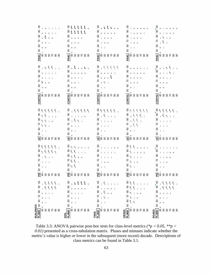
63
Table 3.3: ANOVA pairwise post-hoc tests for class-level metrics (*p < 0.05, **p <
0.01) presented as a cross-tabulation matrix. Pluses and minuses indicate whether the
metric’s value is higher or lower in the subsequent (more recent) decade. Descriptions of
class metrics can be found in Table 3.1.
BU
ILD
ING
S
PL
AN
D50
60
70
80
90
00
PD
50
60
70
80
90
00
IJI
50
60
70
80
90
00
CO
NT
IG50
60
70
80
90
00
FR
AC
50
60
70
80
90
00
40
++
++
––
40–
––
––*
–**
40–
––*
–*
–*
–**
40
++
+*
++
–40–
++
++
–
50
––
––**
–**
50
––
–*
–**
–**
50
––*
–*
–**
–**
50
++
––
–*
50
++
+**
++
60
––
–**
–**
60
––
–**
–**
60
––
––**
60
+–
––**
60
–+
+–
70
––**
–**
70
––**
–**
70
+–
–**
70
––
–**
70
+–
–
80
–**
–**
80
–*
–**
80
––**
80
––
80
––
90
–90
–90
–90
–90
–
SO
IL
PL
AN
D50
60
70
80
90
00
PD
50
60
70
80
90
00
IJI
50
60
70
80
90
00
CO
NT
IG50
60
70
80
90
00
FR
AC
50
60
70
80
90
00
40
++
++
++
40–
–*
–**
–*
–**
–*
40
++
+–
––
40
++
++
++
40
++
++
+**
+**
50
––
–+
+*
50
–**
–**
–**
–**
–*
50
––
–**
––**
50
++
++
+**
50
++
++
**+
**
60
––
++
**60
–+
–+
60
––*
––**
60
––
++
60
++
+**
+**
70
–+
+**
70
+–
+70
––
–**
70
–+
+70
++
**+
**
80
++
**80
––
80
+–**
80
++
*80
+**
+**
90
+90
+90
–**
90
+90
+
TR
EE
PL
AN
D50
60
70
80
90
00
PD
50
60
70
80
90
00
IJI
50
60
70
80
90
00
CO
NT
IG50
60
70
80
90
00
FR
AC
50
60
70
80
90
00
40–
––
––
–40–
––
––
–40–
––
––
–**
40
+–
–+
+–
40–
––
–+
+
50
––*
–**
––**
50
–+
––
–50
––
––**
–**
50
––*
++
–**
50
–+
++
+*
60
–+
+–
60
+–
––
60
––
––**
60
–+
+–**
60
++
++
**
70
++
–70
––
–70
––
–**
70
+**
+–**
70
++
+*
80
––
80
–+
80
––**
80
––**
80
++
90
–90
+90
–90
–**
90
+
GR
AS
S
PL
AN
D50
60
70
80
90
00
PD
50
60
70
80
90
00
IJI
50
60
70
80
90
00
CO
NT
IG50
60
70
80
90
00
FR
AC
50
60
70
80
90
00
40–
–**
–*
–*
–**
–**
40–
–*
–*
–*
–*
–**
40
++
––
––**
40
++
++
++
40–
––
––
–
50
–*
––
–**
–**
50
––
––
–**
50
––**
–**
–**
–**
50
–+
++
+50
–+
++
+
60
++
––
60
+–
––
60
–**
–**
–**
–**
60
++
++
60
++
++
70
+–
–70
––
–70
––**
–**
70
++
+70
–+
+
80
––
80
––
80
––**
80
+–
80
–+
90
–90
–90
–**
90
–90
+
RO
AD
S
PL
AN
D50
60
70
80
90
00
PD
50
60
70
80
90
00
IJI
50
60
70
80
90
00
CO
NT
IG50
60
70
80
90
00
FR
AC
50
60
70
80
90
00
40
++
++
––
40–
––
––
–40–
––
––
–**
40
++
++
++
40
++
––
++
50
+–
––**
–**
50
––
––
–50
––
––**
–**
50
++
+–
–50
––**
–*
––
60
––
–**
–**
60
++
––
60
––
–*
–**
60
+–
––*
60
––
++
70
––**
–**
70
++
–70
––
–**
70
––*
–**
70
++
+
80
–**
–**
80
+–
80
––**
80
––
80
++
90
–90
–90
–90
–90
+
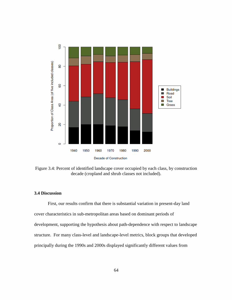
64
Figure 3.4: Percent of identified landscape cover occupied by each class, by construction
decade (cropland and shrub classes not included).
3.4 Discussion
First, our results confirm that there is substantial variation in present-day land
cover characteristics in sub-metropolitan areas based on dominant periods of
development, supporting the hypothesis about path-dependence with respect to landscape
structure. For many class-level and landscape-level metrics, block groups that developed
principally during the 1990s and 2000s displayed significantly different values from
65
earlier-developing regions. These areas tend to differ most significantly from areas that
developed during the 1950s.
By analyzing sprawl across four distinct dimensions (area and density of land
cover, fragmentation/scatter, shape complexity, and diversity), we are able to expand
upon previous studies such as Irwin and Bockstael (2007), Shrestha et al. (2012), and
Zhang et al. (2013). Those studies, using 30m data (which is more adept at detecting
variation between parcels of land), have generally corroborated the traditional
conceptualization of urban sprawl by providing evidence of increased fragmentation near
the urban fringe. Comparison with these studies is complicated by the fact that our results
involve more land cover classes and higher resolution; however, newer-developing areas
in our study do appear more fragmented. Furthermore, landscape patches interface less
frequently with different land cover classes, suggesting that newer-developing areas are
actually more homogenous when we consider several types of land cover (buildings,
roads, trees, grass, soil, shrub, and cropland). While it is not surprising that newer areas
are also less diverse and are covered with fewer roads and buildings, the within-lot land
cover classification that our high-resolution data affords also provides evidence of a shift
from grass and tree covers to soil cover. Shape complexity appears higher in newer areas
as well.
We speculate that certain institutional and economic changes in land use during
the 1990s and 2000s explain some of our results. During the 1960s, commercial uses fled
the downtown area in favor of decentralized office parks, shopping malls, and strip retail
along arterial streets (Luckingham 1989), resulting in a different style of business land
use that not only has a larger footprint but more within-lot variation: shade trees,
66
buildings, grass, and parking may depart more from Euclidean geometry than in a
rectilinear downtown streetscape. Zoning and city ordinances also transformed
residential areas during the latter half of the twentieth century. Increasing minimum lot
sizes for residentially-zoned land, a trend that took place over this period in the Phoenix
area and nationwide (Talen 2012, Fischel 2001) could result in increasing shape
complexity within individual lots, especially when compared to a cookie-cutter 1950s-era
ranch home. Atkinson-Palombo (2010) found that a wider variety of housing types were
present at the urban fringe during the 2000s, which also corroborates some of our results:
a wider variety of building styles could result in increased shape complexity in this
category, while a higher proportion of multifamily housing would result in smaller
building footprints and a lower percent landscape for buildings despite growth in the
number of housing units. Newer construction is also more likely to abut agricultural
lands, which may account for differences in proportional cover as well. In Phoenix, water
rights could play a particularly important role in shaping the extent and pattern of land
cover. Water rights are attached to a particular property and affect the types of irrigation
permitted and cost of water associated with a particular property.
In addition to institutional and economic changes, the development style and
preferences of residents living in Phoenix may also explain why the 1990s and 2000s
zones appear distinctly different. The CBD influenced much of the early development of
Phoenix and still has a great influence on the land use history (Keys et al. 2007). This
could account for similar configurations seen up until the 1990s zones. However, it does
not account for why the 1990s and 2000s zones change so distinctly, particularly in terms
of fragmentation and shape complexity. Further observations show that the development
67
style in Phoenix changes with time. Leapfrog development was a large part of residential
development in American cities between the 1950s and 2000s, particularly in Phoenix
(Helm 2001, Carruthers 2003). This created patches of undeveloped land parcels that
were filled in during later development periods, but it was not until after 1970 that
leapfrogging in Phoenix occurred at greater distances from the CBD (Helm 2001). Based
on our observations, all of these factors are likely to manifest themselves in the
configuration of the 1990s and 2000s zones, where a number of metrics become
significantly different.
Finally, previous research has shown that natives of the Phoenix area seem to
prefer mesic, or grassier, landscaping in backyards in contrast to more recent migrants
who moved to the desert area in droves throughout the second half of the twentieth
century. In addition, preferences for landscaping in Phoenix generally tend to exhibit a
“legacy effect” wherein historically mesic landscape patterns persist in older areas
(Larson et al. 2009). Grass covers are at their highest in the 1940s and 1950s zones.
Grass patch density is highest in the 1940s zone and grass patches less likely to be near
other cover types in newer areas. This may indicate that grasses that do exist in newer-
developing areas are in large open spaces such as parks or golf courses, where patches are
larger and less mixed-in with other land cover types. In contrast, newer areas feature
more soil cover, it is less dense, and its shape complexity is higher, suggesting that
desert-like land cover is more prevalent in backyards than larger public or undeveloped
areas.
3.5 Conclusions
68
Land cover in urban areas is much more complex than the typical sprawl narrative
of increasing fragmentation as one travels toward the urban fringe. The metropolis has
long since ceased to be a monocentric entity; analysis of areas because of some particular
characteristic may be better understood by delineating areas by when they were
developed instead of based on their proximity to the urban core. Results confirm that
sub-metropolitan areas developing principally in different time periods have different
present-day land cover characteristics. Legacy effects and historical development trends
are important to understanding present-day landscape function and ecosystem services.
While evidence suggests that newly-developed areas of Phoenix are less diverse, more
homogenous, and more fragmented, this higher-resolution approach goes beyond these
traditional narratives, finding significant increases in shape complexity and differing
preferences for landscaping in newer-developing areas. Generally speaking, though, these
results corroborate prior research (e.g., Atkinson-Palombo 2010) which has suggested
that the most recent wave of development (1990s and onward) in Phoenix and elsewhere
was distinct from past forms of urban development.
Resolution, both spatial and thematic, remains a very important consideration in
analyzing what constitutes urban sprawl, especially given the increase in data and spatial
analysis tools available. While an ecological understanding of landscape complexity and
arrangement at the 1-m level is not yet as developed owing to the newness of such data,
urbanization and the realization of the importance of urban areas to environmental
outcomes suggest that this is a key area of future research (Turner et al., 2013). The
definition of “fragmentation,” for example, changes whether the research involves only
individual lots, or whether it considers individual trees, sidewalks, and lawn patches. It
69
also changes whether analysis concerns a simple developed/undeveloped dichotomy, or is
attempting to observe more nuanced aspects of urban pattern. The scale of the
aggregation unit merits careful consideration as well. The choice of block groups as units
of analysis was guided principally by theory: it makes sense in Phoenix for analyzing
sub-metropolitan areas that are experienced by individuals, but a different aggregation
unit may make more sense for different levels of spatial or thematic resolution, or if
comparing between different cities. A future study exploring the sensitivity of results to
changes in aggregation units would increase the utility of newly-available high-resolution
data.
While much of our discussion linking landscape change to specific institutional,
economic, and behavioral drivers remains speculative, the approach of linking fine-
resolution land cover to development periods removes the assumption of monocentricity
that is implicit in urban gradient studies and helps to avoid overlooking infill and leapfrog
development patterns. A next step beyond using aggregated information from
FRAGSTATS spatial metrics could use high-resolution land cover classifications to
identify a typology of building and development styles (e.g., ¼-acre lot ranch homes
versus McMansions; strip retail versus mega-malls). Further, an explicit link to
ecological outcomes, such as hydrology or urban heat island, could also move the
discussion toward whether and why certain types of development may be better or worse.
This information and similar analysis can support urban planning in Phoenix and
elsewhere. By analyzing spatial and temporal pattern variation, it is possible to evaluate
the impacts of land use institutions and changing development trends on the overall urban
landscape. Nonetheless, greater understanding of the relationship between pattern and

70
landscape ecology is required to assess the environmental implications of development
types and institutional arrangements. By highlighting spatial pattern differences across
Phoenix, this research hopes to move the discussion of urban landscape pattern beyond
identifying homogeneity and fragmentation and toward an analysis of what it means and
whether it matters.
71
CHAPTER 4
RESIDENTIAL DEVELOPMENT DURING THE GREAT RECESSION
4.1 Introduction
The Real Estate collapse has had a lasting effect on global financial markets, but
these effects have varied across localities. Critical perspectives demonstrate how place-
bound, local financial decision-making – mortgage debt instruments – precipitated a
global financial crisis through the broad redistribution and repackaging of local mortgage
debt via complex financial derivatives (Aalbers 2009, Martin 2010, Crump et al. 2013).
In turn there may be reciprocal effects of the global financial crisis on local development
preferences and patterns. Foreclosure studies provide an early indicator of which
neighborhoods were hit the hardest (Immergluck 2010), but have changes in global
capital availability begun to transform housing choice, and consequently, urban
morphology? Urban theorists have long claimed that “the way people want to live is
more richly varied than post-war suburban planners had imagined,” emphasizing that
zoning and developer behavior have constricted the choice of available housing: fringe
development is not “the product solely of market forces” (Levine 1998). Popular
accounts following the sub-prime collapse proclaim the “death of exurbia” – that the
forces promoting inexpensive, homogenous, car-dependent fringe suburbs are gone and
true preferences for more mixed urbanism – revealed in surveys but not in behavior due
to the limited stock of different housing types – can now be fulfilled (Leinberger 2011).
Developers may respond by reimagining the style and location of housing they supply in
response to changing demographics and individual demands.
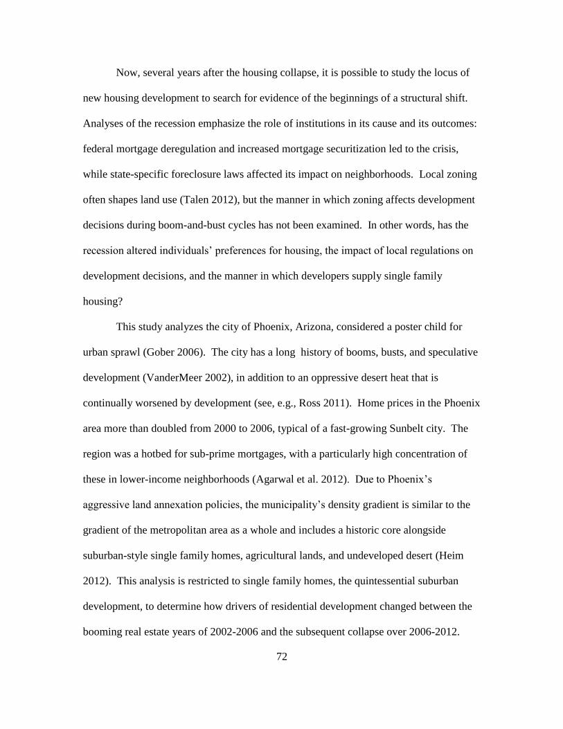
72
Now, several years after the housing collapse, it is possible to study the locus of
new housing development to search for evidence of the beginnings of a structural shift.
Analyses of the recession emphasize the role of institutions in its cause and its outcomes:
federal mortgage deregulation and increased mortgage securitization led to the crisis,
while state-specific foreclosure laws affected its impact on neighborhoods. Local zoning
often shapes land use (Talen 2012), but the manner in which zoning affects development
decisions during boom-and-bust cycles has not been examined. In other words, has the
recession altered individuals’ preferences for housing, the impact of local regulations on
development decisions, and the manner in which developers supply single family
housing?
This study analyzes the city of Phoenix, Arizona, considered a poster child for
urban sprawl (Gober 2006). The city has a long history of booms, busts, and speculative
development (VanderMeer 2002), in addition to an oppressive desert heat that is
continually worsened by development (see, e.g., Ross 2011). Home prices in the Phoenix
area more than doubled from 2000 to 2006, typical of a fast-growing Sunbelt city. The
region was a hotbed for sub-prime mortgages, with a particularly high concentration of
these in lower-income neighborhoods (Agarwal et al. 2012). Due to Phoenix’s
aggressive land annexation policies, the municipality’s density gradient is similar to the
gradient of the metropolitan area as a whole and includes a historic core alongside
suburban-style single family homes, agricultural lands, and undeveloped desert (Heim
2012). This analysis is restricted to single family homes, the quintessential suburban
development, to determine how drivers of residential development changed between the
booming real estate years of 2002-2006 and the subsequent collapse over 2006-2012.
73
This study uses theory from economic geography and a logistic regression at the
parcel-level to empirically analyze these perspectives about residential development and
land use trajectories during the recession. We begin with the tradeoff between access and
space (in the tradition of, e.g., Park, Burgess, McKenzie, & Wirth 1925, Alonso 1964). A
variety of perspectives have stressed the importance of the immediate neighborhood as a
determinant of social outcomes (Sampson 2013), a component of gentrifying cities
(Smith 1996), and as an indicator of walkability and smart growth (Talen 2011), thus we
include counts of parcels by use type within a potential development site’s immediate
vicinity. Zoning is included as it is thought to constrain development decisions by
increasing costs and delaying building. Results provide empirical support for claims
about the changing locus of development resulting from the recession, while the
analytical framework, drawing from traditions in urban economic geography, provides a
fine-grained method for analyzing urban development patterns.
4.2 Literature and Background
4.2.1 The Great Recession
Phoenix has long been known for its booms, busts, and rapidly changing urban
morphology (York et al. 2011a, Kane et al. 2014b). Atkinson-Palombo (2010) notes that
development styles and urban form in Phoenix vary across time periods, finding evidence
of increased density along the urban fringe in the early 2000s which contrasted with the
rapid outward push of single family homes experienced during the nineties. Federal
Reserve data indicate that Arizona housing starts in 2002 increased 15.04% over the
previous year, a trend that continued until 2005, while in 2006 housing starts decreased
by 29.64%. They continued to decrease every year until 2012 (Table 4.1).
74
Table 4.1: Housing starts, state of Arizona
Phoenix’s spectacular booms and busts do not happen in a vacuum – urban
geographers have highlighted the local-global connection of the most recent housing
collapse and recession. Aalbers (2009) describes how a crisis in local housing markets
became a crisis in the global mortgage market. This upscaling, he argues, was the result
of deregulation and the creation of a secondary mortgage market, which allowed agents
to profit from globalizing and financializing a local product. Martin (2010) proposes that
the hyper-fungibility of capital has micro- and macro-geographic impacts, showing that
impacts of the housing collapse were not nationally uniform; instead, they varied between
cities that had “cyclical markets,” “steady markets,” or those characterized as “recent
boomers,” the last of which experienced the highest foreclosure rates. Immergluck
75
(2010) explores the micro-geographical dimension of foreclosures, finding higher rates in
newer and faster-growing ZIP codes, though he was not able to establish a clear
connection between intrametropolitan location and foreclosures specifically, i.e. fringe
development is not clearly implicated in the crisis; if anything, inner cities had higher
rates of bank-owned property. Crump et al. (2013) showcase related equity concerns:
once-redlined neighborhoods became profitable places for subprime mortgages and
subsequently became foreclosure hotspots. For many urban scholars, this recession’s
housing crisis is a symptom of a much deeper and yet unresolved urban crisis, with the
“Growth Machine’s” (Molotch 1976) exclusion mechanisms exhibiting some
vulnerability (Schafran 2013, Harvey 2009). Though this study’s explicit focus is on
land use outcomes rather than the social dimensions of the crisis, critical perspectives
provide useful hypotheses about supply and choice to examine empirically.
The crisis has also been studied by land use economists: Lee (2011) models the
spillover effects of foreclosures on the prices of nearby homes and Cho, Kim and Roberts
(2011) construct a hedonic pricing model to show that the value of environmental
amenities in Nashville, Tennessee decreased slightly following the real estate collapse.
The latter study found an increased preference for housing near the downtown area
following the bust, which the authors hypothesize might be the result of decreased
mobility and disposable income associated with the recession. Finally, some have
pointed out that the recession appears to coincide with demographic trends favoring
walkable, downtown neighborhoods, preferred by the increasing population of empty-
nesters and childless adults (Plane 2013). This suggests a re-evaluation of the type of
76
housing supplied by developers, despite the historically lower risk and ease of
underwriting suburban tract homes (Leinberger and Alfonzo 2012).
4.2.2 Housing supply: Developers and zoning
Urban planners have long claimed that sprawl is the inefficient outcome of an
unregulated market economy (Bruegmann 2005, Whyte 1958). Undifferentiated, single
family housing at the urban fringe is less risky, cheaper to finance (Leinberger and
Alfonzo 2012), and is a standardized product that is easier to produce and absorb in the
market (Peiser 2001). A market failure explanation is often invoked to explain why a
demand for denser urban dwellings may exist but is not realized (Brueckner 2000). In
short, individual choice is often circumscribed by the decisions of developers.
Developers themselves may also be constrained by municipal zoning, which can
restrict available sites or require a costly and time-consuming rezoning process.
American zoning is typically based on a so-called “Euclidean” hierarchy of segregated
land uses, with single family residential areas having very restrictive rules about
permitted uses, followed by higher-density housing, commercial, and finally industrial
land uses that are often lax and allow most higher order uses (Hall 2007). Zoning is
generally treated as an institutional constraint on landowners (Nelson 1977, White 1978,
Fischel 2010). Levine (1998) views land use regulations as constraints on choice which
have for decades “shackled housing markets and ensured standardized outcomes.”
On the other hand, land use outcomes are not necessarily the same as predicted or
intended. Talen (2012) notes the indirectness of the effect of building regulations on
urban form, suggesting that “the effects are known in general terms, on such things as
density and land value, but the effect on physical form and character of place is often
77
obscured,” while Carruthers (2003) argues that the limited nature of zoning and
inconsistent policies across nearby municipalities drive exurbanization and land use
fragmentation. Empirical findings have found that zoning may have a variety of effects.
Glaeser and Gyourko (2002) demonstrate that zoning is partially to blame for the
decreased availability of affordable housing, particularly near increasingly suburban
employment centers, while others have emphasized that zoning’s role in landscape
fragmentation and the protection of natural areas (York and Munroe 2010, Munroe,
Croissant and York 2005).
Because of this, zoning and developer behavior are thought to constrain housing
supply such that it is not perfectly reflective of individual home buyers’ demand. Critical
perspectives suggest that individuals do not have as much variety in housing choice as
they would like while developers are free to manipulate zoning through variances and re-
zonings; thus zoning and development are both reflective of developer preferences (York,
Feiock and Steinacker 2013, Molotch 1979). On the other hand, developers may actually
be constrained by existing homeowners: Fischel (2001) argues that municipal zoning
primarily reflects local homeowners’ interest in protecting the value of their property.
While developers may have some entrepreneurial agency, zoning is likely to pose at least
a procedural inconvenience. Zoning is a major component of where a developer builds a
particular piece of property, though ultimately the decision to develop land is based on a
financial analysis, which would include the cost of any uncertainty or time delays
associated with an unfavorable zoning designation (Reed and Sims 2008).
Preferences revealed through housing choice reflect the interplay of both supply
and demand. At best, they indirectly reflect individual choice, as developers must be
78
sensitive to changing demand for housing, e.g. a reduced preference for fringe
development must eventually result in an increased supply of denser, more centrally-
located homes if nobody were interested in buying the former and they became
unprofitable to supply. In this way, developers must be sensitive to the preferences of
individuals as well as to institutional constraints in order to convert their effort (which
includes, if needed, securing a zoning variance) into return on investment. However, an
individual homebuyer is probably not directly concerned with the price the developer
paid for the land or its original zoning designation.
4.2.3 Housing Demand: Individuals and Place
The aim of this paper is to investigate the changing locus of single family housing
development in Phoenix during the recession. While land prices and zoning may
constrain the quantity and location of housing supplied by a developer, individuals’
preferences for place also have a role in determining where development will take place.
The traditional urban economic model of residential location is based on a tradeoff
between access and space which is little more than a comparison between commuting
time and the size of a home. The decreasing importance of physical distance to fulfill
certain needs (e.g., telecommuting and online shopping), the substitution of square
footage for other forms of consumption such as nearby amenities, and choice of location
based on status all hint at an evolution of preferences beyond this strict dichotomy (Phe
and Wakely 2000). New Urbanists address the social and environmental ills of 20th
century development patterns by emphasizing more compact, sustainable cities with
complementary nearby uses (Talen 2012), while sociologists stress that the
“neighborhood matters” for the reproduction of poverty and education levels across
79
generations (Sampson 2013). Empirically, Carrion-Flores and Irwin (2004) show that the
composition of the immediate neighborhood has a strong spillover effect on the
likelihood of residential development, which they find to be more likely in close
proximity to existing residential or commercial uses.
Urban theorists and critical geographers claiming that there is an oversupply of
suburbia and limited choice in housing type may see the recession as a harbinger of urban
inversion: we may soon witness the “death of the fringe” (Leinberger 2011) or the
advent of “slumburbia” (Schafran 2013). Methods for better understanding these
phenomena might include extensive surveying of stakeholders and decision makers, or
descriptive analyses of select properties or areas. Most empirical approaches toward
residential location involve aggregate geographies such as census tracts (Li, Campbell
and Fernandez 2013), ZIP codes (Immergluck 2010), or even municipalities (Bunel and
Tovar 2013), though results can be highly sensitive to the choice of spatial units. Spatial
representation must follow the data-generating process and urban land use decisions are
made at the parcel level. By directly linking the unit of observation with the decision-
maker, the behavioral component of land-use change can be isolated and used to
reconcile theoretical drivers (processes) with spatially-explicit outcomes (patterns) (Bell
and Irwin 2002, Irwin 2010).
4.3 Empirical Setting
The existing theoretical and empirical literature has demonstrated how aspects of
supply and demand for single family residences may have changed during the recession.
While the distinction between a developer’s criteria for supplying housing and an
individual’s criteria for demanding housing is somewhat artificial, this dichotomy
80
provides a useful starting point for our empirical work. Since developers are thought to
be more sensitive to land cost and institutional setting, our developer/supply model
includes the parcel’s land value in the base year, the land value of surrounding parcels as
a measure of neighborhood wealth, the parcel’s land use type in the base year, and its
zoning designation prior to conversion. Individuals are thought to be more sensitive to
the amenities and place-sensitive characteristics of a potential home, so the
individual/demand model includes population density, the parcel’s distance to the center
of the downtown (CBD), the distance to the nearest of the region’s six edge cities or
subcenters (Garreau 1991, Leslie and Ó hUallacháin 2006), whether it is in walking
distance to Phoenix’s lone light rail line (approved in 2000 and opened in 2008), and its
proximity to other parcels of complementary or incompatible use types. Since Phoenix
has a history of exclusionary housing practices and certain neighborhoods may still be
considered “stigmatized” based on race (Bolin et al. 2005), we also include an area’s
percent White, non-Hispanic. This may affect both a developer’s decision to invest in
housing as well as an individual’s decision to live in an area; we include it in the
individual/demand model so that it is considered alongside other census-derived
variables.
4.3.1 Model specification
This model will determine the probability that a given parcel P1 will convert from
initial land use i to final land use SFR (single family residential) in the final year
conditional on its base year characteristics:
𝑃𝑟(𝑃𝑖1 → 𝑃𝑆𝐹𝑅
1 | 𝑋𝑑1 𝑋𝑠
1)
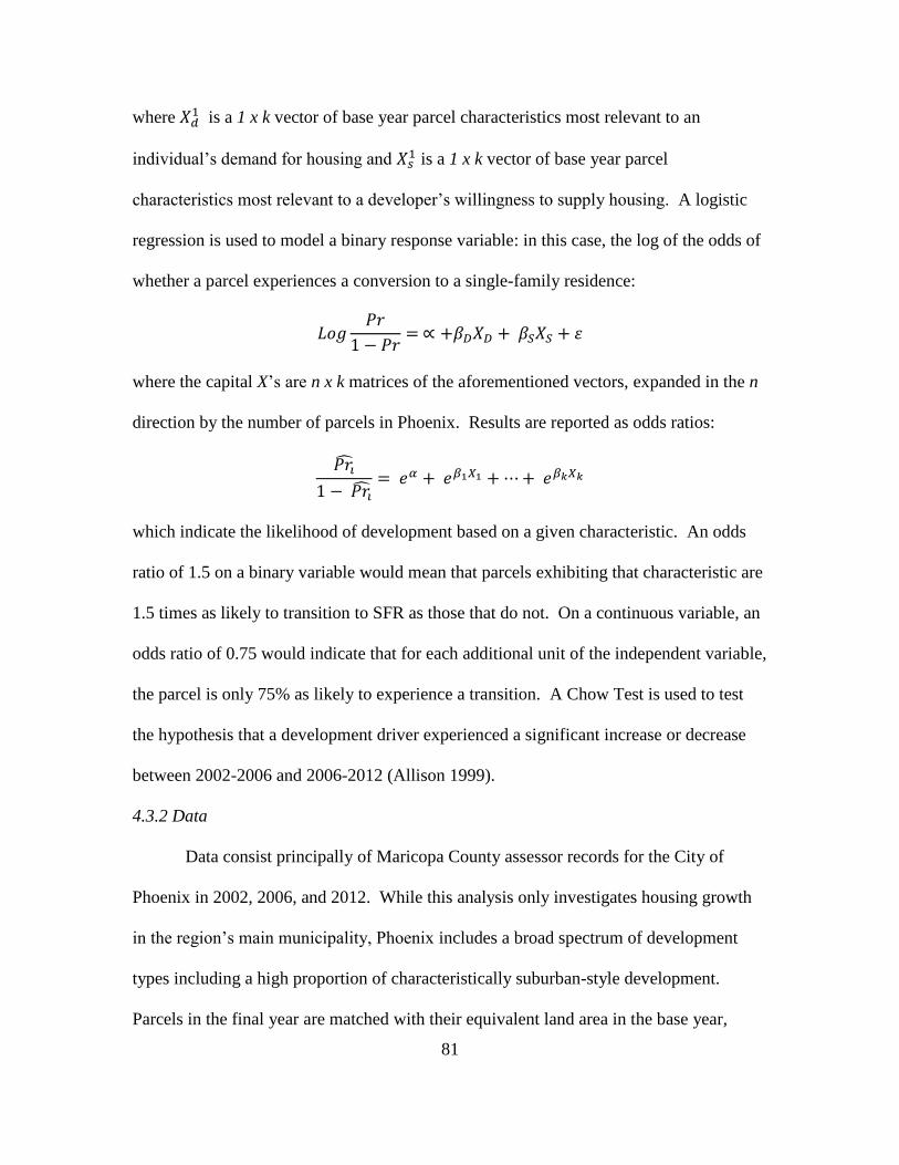
81
where 𝑋𝑑1 is a 1 x k vector of base year parcel characteristics most relevant to an
individual’s demand for housing and 𝑋𝑠1 is a 1 x k vector of base year parcel
characteristics most relevant to a developer’s willingness to supply housing. A logistic
regression is used to model a binary response variable: in this case, the log of the odds of
whether a parcel experiences a conversion to a single-family residence:
𝐿𝑜𝑔𝑃𝑟
1 − 𝑃𝑟= ∝ +𝛽𝐷𝑋𝐷 + 𝛽𝑆𝑋𝑆 + 𝜀
where the capital X’s are n x k matrices of the aforementioned vectors, expanded in the n
direction by the number of parcels in Phoenix. Results are reported as odds ratios:
𝑃𝑟�̂�
1 − 𝑃𝑟�̂�
= 𝑒𝛼 + 𝑒𝛽1𝑋1 + ⋯ + 𝑒𝛽𝑘𝑋𝑘
which indicate the likelihood of development based on a given characteristic. An odds
ratio of 1.5 on a binary variable would mean that parcels exhibiting that characteristic are
1.5 times as likely to transition to SFR as those that do not. On a continuous variable, an
odds ratio of 0.75 would indicate that for each additional unit of the independent variable,
the parcel is only 75% as likely to experience a transition. A Chow Test is used to test
the hypothesis that a development driver experienced a significant increase or decrease
between 2002-2006 and 2006-2012 (Allison 1999).
4.3.2 Data
Data consist principally of Maricopa County assessor records for the City of
Phoenix in 2002, 2006, and 2012. While this analysis only investigates housing growth
in the region’s main municipality, Phoenix includes a broad spectrum of development
types including a high proportion of characteristically suburban-style development.
Parcels in the final year are matched with their equivalent land area in the base year,
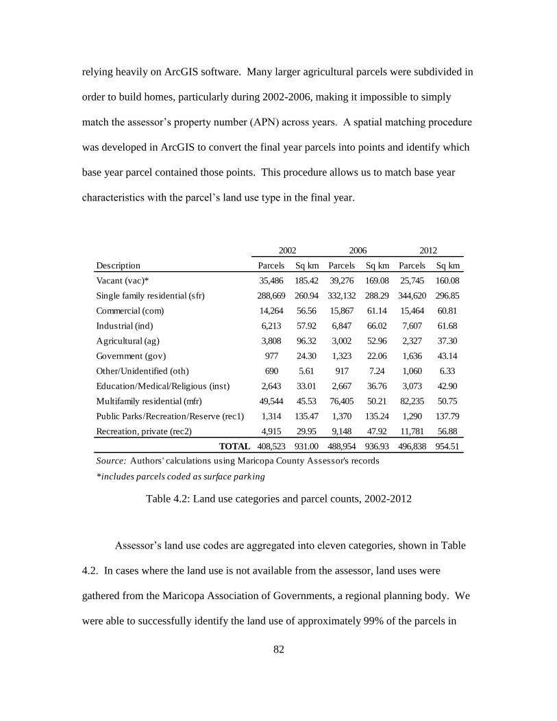
82
relying heavily on ArcGIS software. Many larger agricultural parcels were subdivided in
order to build homes, particularly during 2002-2006, making it impossible to simply
match the assessor’s property number (APN) across years. A spatial matching procedure
was developed in ArcGIS to convert the final year parcels into points and identify which
base year parcel contained those points. This procedure allows us to match base year
characteristics with the parcel’s land use type in the final year.
Table 4.2: Land use categories and parcel counts, 2002-2012
Assessor’s land use codes are aggregated into eleven categories, shown in Table
4.2. In cases where the land use is not available from the assessor, land uses were
gathered from the Maricopa Association of Governments, a regional planning body. We
were able to successfully identify the land use of approximately 99% of the parcels in
Description Parcels Sq km Parcels Sq km Parcels Sq km
Vacant (vac)* 35,486 185.42 39,276 169.08 25,745 160.08
Single family residential (sfr) 288,669 260.94 332,132 288.29 344,620 296.85
Commercial (com) 14,264 56.56 15,867 61.14 15,464 60.81
Industrial (ind) 6,213 57.92 6,847 66.02 7,607 61.68
Agricultural (ag) 3,808 96.32 3,002 52.96 2,327 37.30
Government (gov) 977 24.30 1,323 22.06 1,636 43.14
Other/Unidentified (oth) 690 5.61 917 7.24 1,060 6.33
Education/Medical/Religious (inst) 2,643 33.01 2,667 36.76 3,073 42.90
Multifamily residential (mfr) 49,544 45.53 76,405 50.21 82,235 50.75
Public Parks/Recreation/Reserve (rec1) 1,314 135.47 1,370 135.24 1,290 137.79
Recreation, private (rec2) 4,915 29.95 9,148 47.92 11,781 56.88
TOTAL 408,523 931.00 488,954 936.93 496,838 954.51
Source: Authors' calculations using Maricopa County Assessor's records
*includes parcels coded as surface parking
2002 20122006
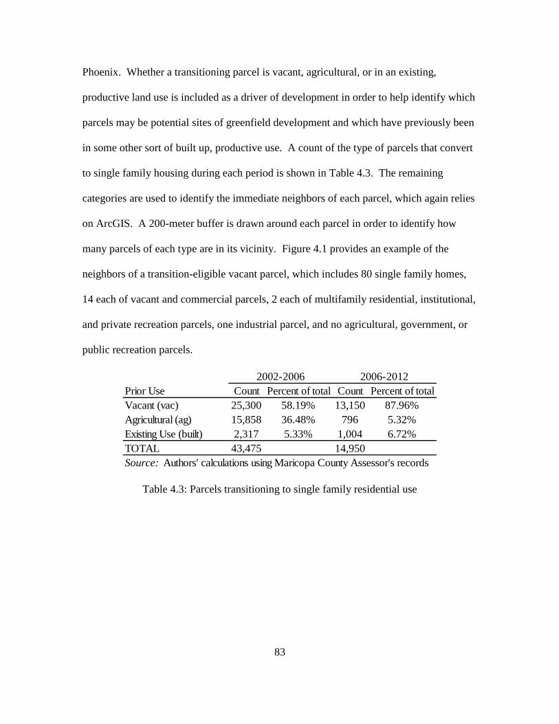
83
Phoenix. Whether a transitioning parcel is vacant, agricultural, or in an existing,
productive land use is included as a driver of development in order to help identify which
parcels may be potential sites of greenfield development and which have previously been
in some other sort of built up, productive use. A count of the type of parcels that convert
to single family housing during each period is shown in Table 4.3. The remaining
categories are used to identify the immediate neighbors of each parcel, which again relies
on ArcGIS. A 200-meter buffer is drawn around each parcel in order to identify how
many parcels of each type are in its vicinity. Figure 4.1 provides an example of the
neighbors of a transition-eligible vacant parcel, which includes 80 single family homes,
14 each of vacant and commercial parcels, 2 each of multifamily residential, institutional,
and private recreation parcels, one industrial parcel, and no agricultural, government, or
public recreation parcels.
Table 4.3: Parcels transitioning to single family residential use
Prior Use Count Percent of total Count Percent of total
Vacant (vac) 25,300 58.19% 13,150 87.96%
Agricultural (ag) 15,858 36.48% 796 5.32%
Existing Use (built) 2,317 5.33% 1,004 6.72%
TOTAL 43,475 14,950
Source: Authors' calculations using Maricopa County Assessor's records
2002-2006 2006-2012
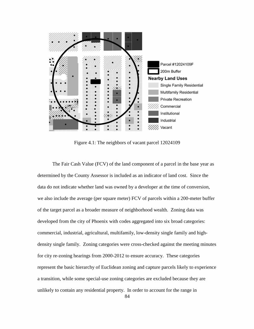
84
Figure 4.1: The neighbors of vacant parcel 12024109
The Fair Cash Value (FCV) of the land component of a parcel in the base year as
determined by the County Assessor is included as an indicator of land cost. Since the
data do not indicate whether land was owned by a developer at the time of conversion,
we also include the average (per square meter) FCV of parcels within a 200-meter buffer
of the target parcel as a broader measure of neighborhood wealth. Zoning data was
developed from the city of Phoenix with codes aggregated into six broad categories:
commercial, industrial, agricultural, multifamily, low-density single family and high-
density single family. Zoning categories were cross-checked against the meeting minutes
for city re-zoning hearings from 2000-2012 to ensure accuracy. These categories
represent the basic hierarchy of Euclidean zoning and capture parcels likely to experience
a transition, while some special-use zoning categories are excluded because they are
unlikely to contain any residential property. In order to account for the range in
85
allowable density within single family residential zoning, we split this category at a
threshold of ¼-acre per dwelling unit, below which per square foot land values increase
substantially.
Other variables were also created using ArcGIS. The population density and
percent White, non-Hispanic population are that of the census tract in which the parcel
lies, using 2000 U.S. Census figures for the 2002-2006 model and 2005-2009 American
Community Survey five-year estimates for the 2006-2012 model. In order to better
interpret logistic regression results, population density is treated as a binary variable,
taking a value of 1 if the parcel lies in a tract with above average population density and 0
otherwise (1824 people/sq. km in 2000 and 1799 people/sq. km in 2005-2009).
Phoenix’s light rail line was approved by voters in 2000 and opened in 2008, though
special transit-oriented districts were created near station sites as early as 2003 in
anticipation of nearby construction (Golub, Guhathakurta and Sollapuram 2012). The
transit access variable takes a value of 1 if the parcel is within walking distance (800
meters) of a light rail station and 0 otherwise.
4.4 Descriptive Results
Careful analysis of the conversion data provides numerous insights. Table 4.2
shows the relative hegemony of single family housing in Phoenix, which makes up close
to 70% of the parcels and 30% of the city’s land area in any given year. Perhaps most
striking is the decrease in conversions from 43,475 to 14,950 (Table 4.3), which
corroborates the statewide housing starts data presented in Table 4.1. The prior use of
transitioning parcels also changes dramatically. During the boom, conversions to single
family took place on a blend of agricultural land (36% of parcels), vacant land (58%),
86
and previously built land (5%) while during the recession the percent of conversions
taking place on agricultural land dropped precipitously (5%), vacant represented most of
the conversions (88%), and built increased slightly (7%). While the drop in agricultural
conversions is steep, parcels transitioning from agricultural to SFR often undergo an
intermediate vacant classification. During the bust, existing vacant land that had been
cleared was far more likely to be utilized for SFR construction versus further attempts to
clear agricultural land for development.
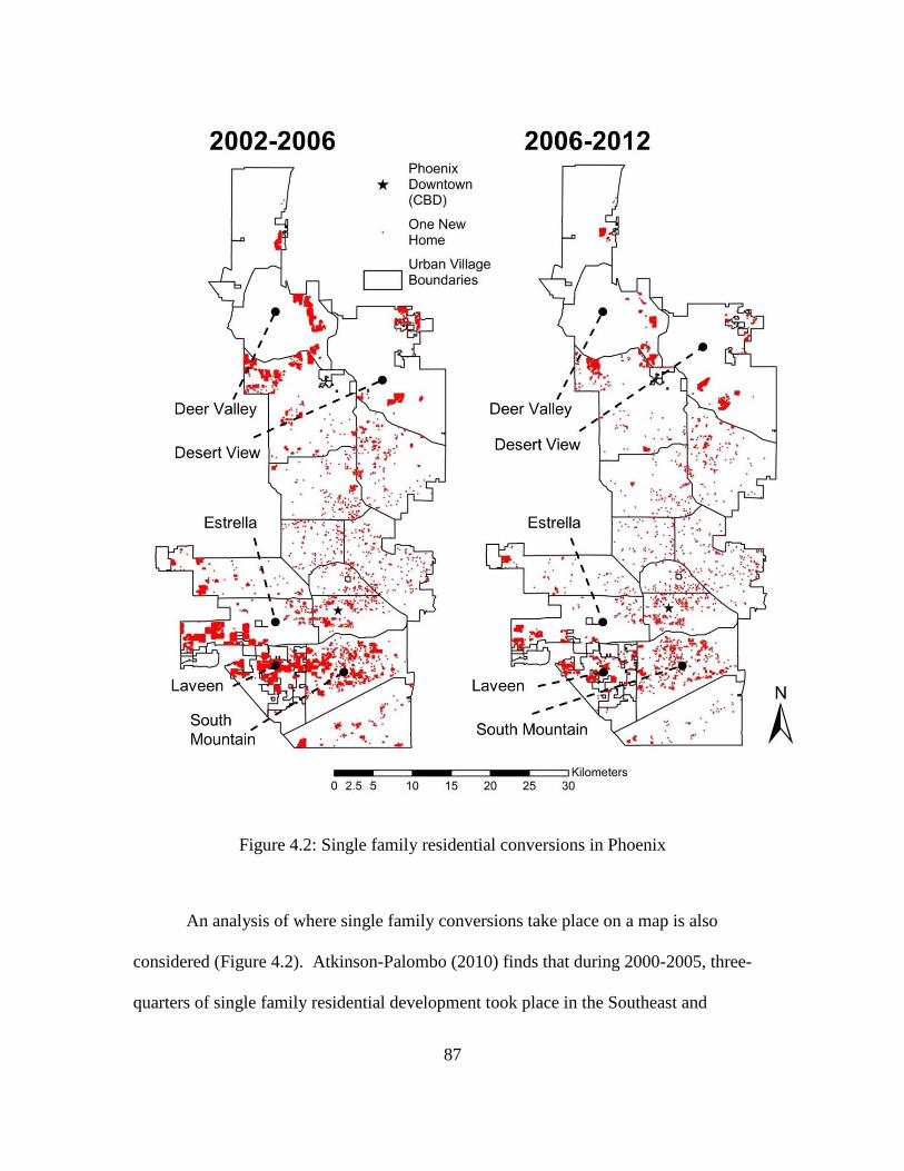
87
Figure 4.2: Single family residential conversions in Phoenix
An analysis of where single family conversions take place on a map is also
considered (Figure 4.2). Atkinson-Palombo (2010) finds that during 2000-2005, three-
quarters of single family residential development took place in the Southeast and
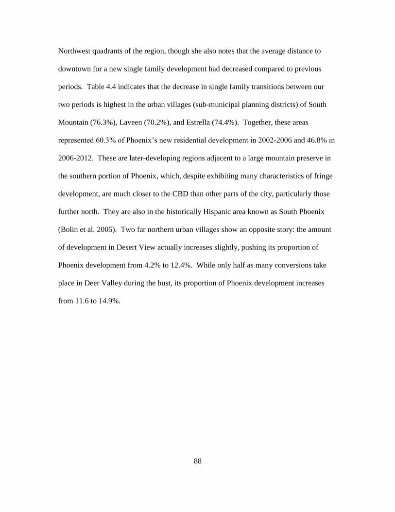
88
Northwest quadrants of the region, though she also notes that the average distance to
downtown for a new single family development had decreased compared to previous
periods. Table 4.4 indicates that the decrease in single family transitions between our
two periods is highest in the urban villages (sub-municipal planning districts) of South
Mountain (76.3%), Laveen (70.2%), and Estrella (74.4%). Together, these areas
represented 60.3% of Phoenix’s new residential development in 2002-2006 and 46.8% in
2006-2012. These are later-developing regions adjacent to a large mountain preserve in
the southern portion of Phoenix, which, despite exhibiting many characteristics of fringe
development, are much closer to the CBD than other parts of the city, particularly those
further north. They are also in the historically Hispanic area known as South Phoenix
(Bolin et al. 2005). Two far northern urban villages show an opposite story: the amount
of development in Desert View actually increases slightly, pushing its proportion of
Phoenix development from 4.2% to 12.4%. While only half as many conversions take
place in Deer Valley during the bust, its proportion of Phoenix development increases
from 11.6 to 14.9%.
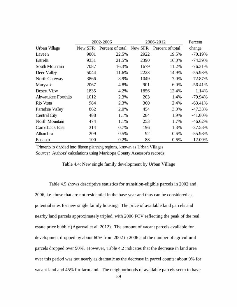
89
Table 4.4: New single family development by Urban Village
Table 4.5 shows descriptive statistics for transition-eligible parcels in 2002 and
2006, i.e. those that are not residential in the base year and thus can be considered as
potential sites for new single family housing. The price of available land parcels and
nearby land parcels approximately tripled, with 2006 FCV reflecting the peak of the real
estate price bubble (Agarwal et al. 2012). The amount of vacant parcels available for
development dropped by about 60% from 2002 to 2006 and the number of agricultural
parcels dropped over 90%. However, Table 4.2 indicates that the decrease in land area
over this period was not nearly as dramatic as the decrease in parcel counts: about 9% for
vacant land and 45% for farmland. The neighborhoods of available parcels seem to have
Percent
Urban Village New SFR Percent of total New SFR Percent of total change
Laveen 9801 22.5% 2922 19.5% -70.19%
Estrella 9331 21.5% 2390 16.0% -74.39%
South Mountain 7087 16.3% 1679 11.2% -76.31%
Deer Valley 5044 11.6% 2223 14.9% -55.93%
North Gateway 3866 8.9% 1049 7.0% -72.87%
Maryvale 2067 4.8% 901 6.0% -56.41%
Desert View 1835 4.2% 1856 12.4% 1.14%
Ahwatukee Foothills 1012 2.3% 203 1.4% -79.94%
Rio Vista 984 2.3% 360 2.4% -63.41%
Paradise Valley 862 2.0% 454 3.0% -47.33%
Central City 488 1.1% 284 1.9% -41.80%
North Mountain 474 1.1% 253 1.7% -46.62%
Camelback East 314 0.7% 196 1.3% -37.58%
Alhambra 209 0.5% 92 0.6% -55.98%
Encanto 100 0.2% 88 0.6% -12.00%aPhoenix is divided into fifteen planning regions, known as Urban Villages
Source: Authors' calculations using Maricopa County Assessor's records
2002-2006 2006-2012

90
changed too – parcels that remain transition-eligible by 2006 tend to be surrounded by
more vacant parcels, multifamily residential, and commercial parcels and less likely to be
near agriculture. On average, available parcels are slightly closer to the downtown and to
subcenters.
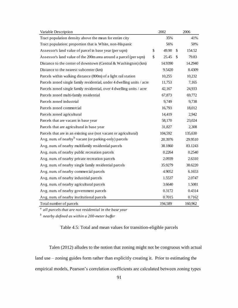
91
Table 4.5: Total and mean values for transition-eligible parcels
Talen (2012) alludes to the notion that zoning might not be congruous with actual
land use – zoning guides form rather than explicitly creating it. Prior to estimating the
empirical models, Pearson’s correlation coefficients are calculated between zoning types
Variable Description 2002 2006
Tract population density above the mean for entire city 35% 41%
Tract population: proportion that is White, non-Hispanic 56% 50%
Assessor's land value of parcel in base year (per sqm) 49.90$ 154.52$
Assessor's land value of the 200m area around a parcel (per sqm) 25.45$ 79.83$
Distance to the center of downtown (Central & Washington) (km) 14.9390 14.2940
Distance to the nearest subcenter (km) 9.5420 8.4309
Parcels within walking distance (800m) of a light rail station 10,255 10,232
Parcels zoned single family residential, under 4 dwelling units / acre 11,753 7,165
Parcels zoned single family residential, over 4 dwelling units / acre 42,167 24,933
Parcels zoned multi-family residential 67,873 69,772
Parcels zoned industrial 9,749 9,738
Parcels zoned commercial 16,793 18,012
Parcels zoned agricultural 14,419 2,942
Parcels that are vacant in base year 58,170 23,024
Parcels that are agricultural in base year 31,827 2,308
Parcels that are in an existing use (not vacant or agricultural) 104,592 135,630
Avg. num. of nearbyb vacant (or parking-only) parcels 20.3976 29.9510
Avg. num. of nearby multifamily residential parcels 38.1860 83.1243
Avg. num. of nearby public recreation parcels 0.2264 0.2540
Avg. num. of nearby private recreation parcels 2.0939 2.6310
Avg. num. of nearby single family residential parcels 35.9279 38.6220
Avg. num. of nearby commercial parcels 4.9052 6.1653
Avg. num. of nearby industrial parcels 1.5537 2.0747
Avg. num. of nearby agricultural parcels 3.6640 1.5081
Avg. num. of nearby government parcels 0.3172 0.4314
Avg. num. of nearby institutional parcels 0.7015 0.7162
Total number of parcels 194,589 160,962 a
all parcels that are not residential in the base year
b nearby defined as within a 200-meter buffer
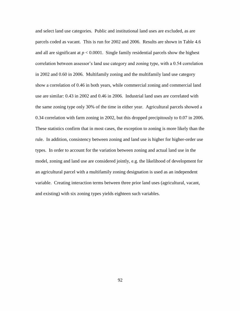
92
and select land use categories. Public and institutional land uses are excluded, as are
parcels coded as vacant. This is run for 2002 and 2006. Results are shown in Table 4.6
and all are significant at p < 0.0001. Single family residential parcels show the highest
correlation between assessor’s land use category and zoning type, with a 0.54 correlation
in 2002 and 0.60 in 2006. Multifamily zoning and the multifamily land use category
show a correlation of 0.46 in both years, while commercial zoning and commercial land
use are similar: 0.43 in 2002 and 0.46 in 2006. Industrial land uses are correlated with
the same zoning type only 30% of the time in either year. Agricultural parcels showed a
0.34 correlation with farm zoning in 2002, but this dropped precipitously to 0.07 in 2006.
These statistics confirm that in most cases, the exception to zoning is more likely than the
rule. In addition, consistency between zoning and land use is higher for higher-order use
types. In order to account for the variation between zoning and actual land use in the
model, zoning and land use are considered jointly, e.g. the likelihood of development for
an agricultural parcel with a multifamily zoning designation is used as an independent
variable. Creating interaction terms between three prior land uses (agricultural, vacant,
and existing) with six zoning types yields eighteen such variables.
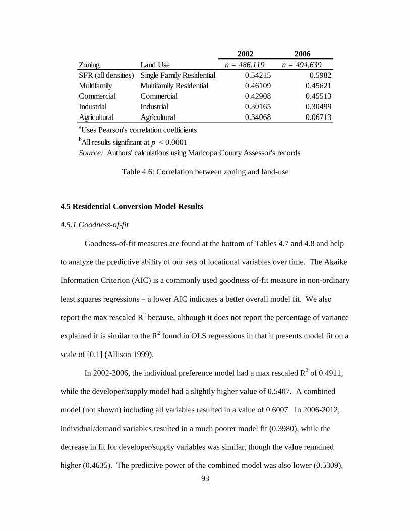
93
Table 4.6: Correlation between zoning and land-use
4.5 Residential Conversion Model Results
4.5.1 Goodness-of-fit
Goodness-of-fit measures are found at the bottom of Tables 4.7 and 4.8 and help
to analyze the predictive ability of our sets of locational variables over time. The Akaike
Information Criterion (AIC) is a commonly used goodness-of-fit measure in non-ordinary
least squares regressions – a lower AIC indicates a better overall model fit. We also
report the max rescaled R2 because, although it does not report the percentage of variance
explained it is similar to the R2 found in OLS regressions in that it presents model fit on a
scale of [0,1] (Allison 1999).
In 2002-2006, the individual preference model had a max rescaled R2 of 0.4911,
while the developer/supply model had a slightly higher value of 0.5407. A combined
model (not shown) including all variables resulted in a value of 0.6007. In 2006-2012,
individual/demand variables resulted in a much poorer model fit (0.3980), while the
decrease in fit for developer/supply variables was similar, though the value remained
higher (0.4635). The predictive power of the combined model was also lower (0.5309).
2002 2006
Zoning Land Use n = 486,119 n = 494,639
SFR (all densities) Single Family Residential 0.54215 0.5982
Multifamily Multifamily Residential 0.46109 0.45621
Commercial Commercial 0.42908 0.45513
Industrial Industrial 0.30165 0.30499
Agricultural Agricultural 0.34068 0.06713aUses Pearson's correlation coefficients
bAll results significant at p < 0.0001
Source: Authors' calculations using Maricopa County Assessor's records

94
Overall, the same set of variables do a poorer job explaining the likelihood of parcels
developing during the recession, indicating a larger role for external factors not included
in the model, such as credit availability which exists at a larger scale than the
metropolitan area but may have differentially affected parcels across the study site.
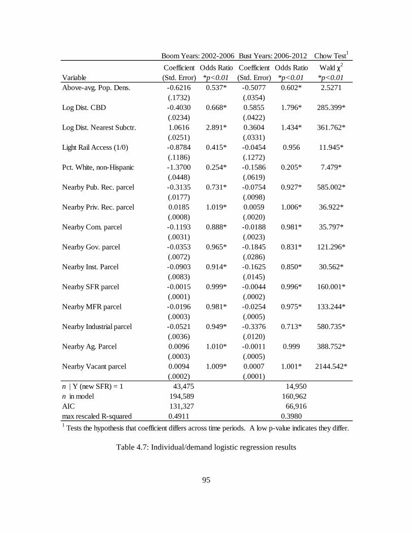
95
Table 4.7: Individual/demand logistic regression results
Chow Test1
Coefficient Odds Ratio Coefficient Odds Ratio Wald χ2
Variable (Std. Error) *p<0.01 (Std. Error) *p<0.01 *p<0.01
Above-avg. Pop. Dens. -0.6216 0.537* -0.5077 0.602* 2.5271
(.1732) (.0354)
Log Dist. CBD -0.4030 0.668* 0.5855 1.796* 285.399*
(.0234) (.0422)
Log Dist. Nearest Subctr. 1.0616 2.891* 0.3604 1.434* 361.762*
(.0251) (.0331)
Light Rail Access (1/0) -0.8784 0.415* -0.0454 0.956 11.945*
(.1186) (.1272)
Pct. White, non-Hispanic -1.3700 0.254* -0.1586 0.205* 7.479*
(.0448) (.0619)
Nearby Pub. Rec. parcel -0.3135 0.731* -0.0754 0.927* 585.002*
(.0177) (.0098)
Nearby Priv. Rec. parcel 0.0185 1.019* 0.0059 1.006* 36.922*
(.0008) (.0020)
Nearby Com. parcel -0.1193 0.888* -0.0188 0.981* 35.797*
(.0031) (.0023)
Nearby Gov. parcel -0.0353 0.965* -0.1845 0.831* 121.296*
(.0072) (.0286)
Nearby Inst. Parcel -0.0903 0.914* -0.1625 0.850* 30.562*
(.0083) (.0145)
Nearby SFR parcel -0.0015 0.999* -0.0044 0.996* 160.001*
(.0001) (.0002)
Nearby MFR parcel -0.0196 0.981* -0.0254 0.975* 133.244*
(.0003) (.0005)
Nearby Industrial parcel -0.0521 0.949* -0.3376 0.713* 580.735*
(.0036) (.0120)
Nearby Ag. Parcel 0.0096 1.010* -0.0011 0.999 388.752*
(.0003) (.0005)
Nearby Vacant parcel 0.0094 1.009* 0.0007 1.001* 2144.542*
(.0002) (.0001)
n | Y (new SFR) = 1 43,475 14,950
n in model 194,589 160,962
AIC 131,327 66,916
max rescaled R-squared 0.4911 0.39801
Tests the hypothesis that coefficient differs across time periods. A low p-value indicates they differ.
Boom Years: 2002-2006 Bust Years: 2006-2012
96
4.5.2 Individuals and demand
Results for the individual/demand model are found in Table 4.7. Owing to the
large number of observations – nearly half a million parcels in total – almost all estimates
are significant at the p < 0.01 level. The dependent variable is the log-likelihood of
whether or not a parcel experiences a transition to SFR. Odds ratios are a convenient
way of analyzing the marginal contribution of a dependent variable, while the Chow Test
reveals whether a variable was significantly different between the boom period (2002-
2006) and the bust period (2006-2012). We hypothesized, based on theories of “urban
inversion,” increased commuting costs, and an increased awareness of sustainable
development that individuals’ preferences for housing during the recession would shift
toward areas demonstrating complementary land uses, areas nearer their potential places
of recreation, shopping, and work (CBD and subcenters), those with a higher population
density, and near the recently completed light rail line.
Being in a census tract with an above-average population density is a negative
predictor of development during both the boom (0.537) and the bust (0.602) and change
over time is not significant. The variables indicating the distance to downtown and
subcenters are interpreted as “the impact of additional distance,” so the 0.668 odds ratio
in 2002-2006 indicates that being farther from downtown was a negative development
predictor. Contrary to the idea of “urban inversion,” additional distance from downtown
substantially increases the likelihood that a parcel will develop after the bust, so much
that this strong negative predictor becomes strongly positive (1.796). The region’s
subcenters, three of which are located outside Phoenix’s city limits, show the opposite
effect: being far from a subcenter began as a strong predictor of development (2.891
97
times as likely to develop for each additional log mile); during the bust its impact is
lessened (1.434 times as likely for each additional log mile) and subcenter proximity
became less unattractive.
Whether a parcel was within walking distance from a (then-proposed) light rail
station was a strong negative predictor of development during the boom years – all other
things equal, it was far less likely for a parcel near a train station to become single family
housing. This odds ratio climbs to nearly 1 during the bust and although its impact is not
clear, it is significantly different from the prior period. Essentially, proximity to the train
no longer “repels” single family development. The percent of the population that is
White, non-Hispanic is negatively related to development during both periods, and
parcels in areas with low minority populations were even less likely to develop during the
bust years. It appears that Phoenix may actually be exhibiting “inclusionary”
development. Alternatively, this could be an indicator of gentrifying pressures within
historically minority areas of the city, perhaps consistent with a “third wave” of
gentrification which tends to take place when developers capitalize on cheap property
values during a recession in order to turn a neighborhood (Hackworth and Smith 2001).
The remaining variables in the individual/demand model measure the marginal
contribution of a single, nearby parcel of a particular type to the likelihood of
development. They can represent spatial externalities such as the positive impact of
nearby schools, parks, or grocery stores, or the negative externalities associated with
nearby industry. Measuring the impact of other parcels under development can indicate
the spillover effects of nearby development: during a boom, being near a hot new area
might be seen as a positive, but in a recession a nearby foreclosed home or unfinished
98
property could be very undesirable. Some of the categories available in this study do not
have the granularity needed to hypothesize whether a nearby parcel would be desired or
undesired near a home, specifically for government, commercial, and certain institutional
parcels. A neighborhood grocery or coffee shop, an amenity for many individuals, is
indistinguishable from a big-box store or a large suburban office park in this data.
Nonetheless, some trends are clear. Nearby public recreation, which consists
primarily of city parks and mountain preserves, is a significant negative predictor of
development (0.731), but its repellent effect decreases dramatically during the bust (to
0.931) indicating that a nearby park is seen much more favorably as far as residential
location is concerned. Nearby private recreation, which consists primarily of golf courses
or common spaces in homeowners’ associations, is decreasingly valued, though even in
the bust its odds ratio is still slightly above one. Nearby commercial parcels show a
similar trend, at first exhibiting a significant, negative odds ratio (0.888), but becoming
decreasingly repellent during the bust (0.981). To the extent that these represent
walkable grocery stores or offices, this would be welcome news to New Urbanists – even
a decreasing negative effect for larger commercial establishments like big-box retail
would indicate an increased preference for land use heterogeneity. While multifamily
developments are often thought to be undesirable attractors of low-income individuals,
congestion, and crime (Park, Kwon, & Lee, 2013), results show that proximity to such
parcels is only slightly dis-favored, but the repellent effect increases somewhat during the
recession. The repellent effect of nearby industry increases dramatically (from 0.949 to
0.713), indicating people may be more willing or able to avoid this negative externality.
Finally, the impacts of nearby agricultural or vacant parcels decrease modestly, indicating

99
that parcels near unbuilt or developable land are less likely to convert to housing during
the recession than previously.
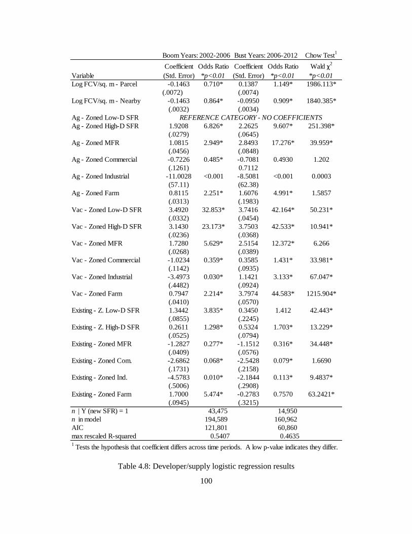
100
Table 4.8: Developer/supply logistic regression results
Chow Test1
Coefficient Odds Ratio Coefficient Odds Ratio Wald χ2
Variable (Std. Error) *p<0.01 (Std. Error) *p<0.01 *p<0.01
Log FCV/sq. m - Parcel -0.1463 0.710* 0.1387 1.149* 1986.113*
(.0072) (.0074)
Log FCV/sq. m - Nearby -0.1463 0.864* -0.0950 0.909* 1840.385*
(.0032) (.0034)
Ag - Zoned Low-D SFR
Ag - Zoned High-D SFR 1.9208 6.826* 2.2625 9.607* 251.398*
(.0279) (.0645)
Ag - Zoned MFR 1.0815 2.949* 2.8493 17.276* 39.959*
(.0456) (.0848)
Ag - Zoned Commercial -0.7226 0.485* -0.7081 0.4930 1.202
(.1261) 0.7112
Ag - Zoned Industrial -11.0028 <0.001 -8.5081 <0.001 0.0003
(57.11) (62.38)
Ag - Zoned Farm 0.8115 2.251* 1.6076 4.991* 1.5857
(.0313) (.1983)
Vac - Zoned Low-D SFR 3.4920 32.853* 3.7416 42.164* 50.231*
(.0332) (.0454)
Vac - Zoned High-D SFR 3.1430 23.173* 3.7503 42.533* 10.941*
(.0236) (.0368)
Vac - Zoned MFR 1.7280 5.629* 2.5154 12.372* 6.266
(.0268) (.0389)
Vac - Zoned Commercial -1.0234 0.359* 0.3585 1.431* 33.981*
(.1142) (.0935)
Vac - Zoned Industrial -3.4973 0.030* 1.1421 3.133* 67.047*
(.4482) (.0924)
Vac - Zoned Farm 0.7947 2.214* 3.7974 44.583* 1215.904*
(.0410) (.0570)
Existing - Z. Low-D SFR 1.3442 3.835* 0.3450 1.412 42.443*
(.0855) (.2245)
Existing - Z. High-D SFR 0.2611 1.298* 0.5324 1.703* 13.229*
(.0525) (.0794)
Existing - Zoned MFR -1.2827 0.277* -1.1512 0.316* 34.448*
(.0409) (.0576)
Existing - Zoned Com. -2.6862 0.068* -2.5428 0.079* 1.6690
(.1731) (.2158)
Existing - Zoned Ind. -4.5783 0.010* -2.1844 0.113* 9.4837*
(.5006) (.2908)
Existing - Zoned Farm 1.7000 5.474* -0.2783 0.7570 63.2421*
(.0945) (.3215)
n | Y (new SFR) = 1 43,475 14,950
n in model 194,589 160,962
AIC 121,801 60,860
max rescaled R-squared 0.5407 0.46351
Tests the hypothesis that coefficient differs across time periods. A low p-value indicates they differ.
Boom Years: 2002-2006 Bust Years: 2006-2012
REFERENCE CATEGORY - NO COEFFICIENTS
101
4.5.3 Developers and supply
The second model is shown in Table 4.8 and analyzes development based on
factors pertaining to developer behavior and the supply of housing. Theories about an
“oversupply of suburbia” would suggest that greenfield development on inexpensive land
that is already zoned for single family homes would be the most likely to develop,
particularly during the boom years. Descriptive results, which excluded vacant parcels,
showed that zoning is often incongruous with actual land use and that this incongruity
became more pronounced during the bust for agricultural land. The average assessor’s
fair cash value (FCV) of transition-eligible parcels was much higher in 2006 than in
2002, reflecting the housing bubble.
Development is more likely on cheaper parcels of land during the boom, with an
odds ratio of 0.71 on FCV per square meter. A negative, though less extreme effect, is
seen for land prices within a 200m buffer of the transitioning parcel (0.864). During the
bust, the repellent effect of pricier nearby land is slightly decreased (to 0.909) though a
high price of the parcel itself actually becomes a positive predictor of development
(1.149). These are the most significant changes of any coefficients. This appears to
reflect increased risk-aversion on the part of developers, with a shift away from seeking
speculative gains in low-value areas during the boom in favor of development in already
desirable neighborhoods.
The jointly-modeled effects of prior use and zoning are more difficult to
disentangle than other development drivers, but the predictive ability of these interaction
variables is reflected in the model’s relatively high goodness-of-fit. Odds ratios for these
variables must be interpreted relative to the reference category, which was chosen as
102
agricultural land zoned for low density, single family residences, i.e. the likelihood of
some other use type developing is presented relative to large-lot greenfield development
of former farmland. For agricultural land, higher-density zoning is preferred to lower-
density zoning and this effect strengthens significantly during the recession (6.826 to
9.607). Agricultural land with a multifamily zoning designation (which does allow for
higher-density single family housing in some circumstances) was very unlikely to
develop during the boom years, but the odds ratio increases dramatically thereafter (0.485
to 17.276). We hypothesize that commercial or industrial zoned parcels, regardless of
use type, only convert to single family homes in somewhat unusual cases, such as the
“rescuing” of a previous, failed development or an one-time (but major) change in local
land use plans. We do not believe that this model, which only considers mean effects,
reflects any particularly strong trends in such idiosyncratic cases. Farmland that retains
agricultural zoning is more likely to develop than low-density single family zoned
agricultural land, but less likely than most other categories. This does not change
significantly during the recession, leading to the belief that an agricultural zoning
designation slows some farmland conversion in comparison to farmland zoned for other
uses, though not all.
Parcels designated as vacant are more likely to develop than agricultural land in
most cases – a distinction that increases substantially in the bust, during which vacant
land dramatically overshadowed agricultural land as the use type most likely to develop.
During the boom, low-density zoned vacant parcels are more likely to develop than their
higher-density zoned counterparts (32.853 vs. 23.173), though in the recession the
difference between the two becomes negligible (42.164 vs. 42.533). The shift away from
103
development on lower-density zoned land is true for existing parcels as well. As was true
for farmland, development is also increasingly likely on multifamily zoned vacant land
(5.629 to 12.372). We can only speculate that the high odds ratio on already built, farm-
zoned land during the boom is reflective of a handful of peculiar cases; it decreases and
becomes insignificant during the bust.
4.6 Discussion
This study analyzes how drivers of single family residential development changed
during the recession. The analysis was structured around a distinction between drivers of
housing supply (developer behavior and the constraint presented by zoning) and housing
demand (individuals and their preference for place) whilst seeking to gain an empirical
understanding of the contention that the recession may be fundamentally changing urban
development patterns.
Considering Phoenix’s historical development trajectory, the drivers of new
housing from 2002-2006 are not unexpected: lower-cost, lower-density areas on
converted farmland in the interstices between the region’s subcenters are likely to
develop. However, the seemingly inverted results for distance to downtown (positive
predictor) and distance to subcenters (negative predictor) need to be interpreted with
caution due to the city’s layout. The urban villages of South Mountain, Laveen, and
Estrella have already been identified as representing a sizeable component of boom-era
greenfield development (Table 4.4). These areas have smaller parcel sizes compared to
those at the urban periphery as well as historic minority and low-income populations,
making them less attractive to large developers until the early 2000s when they first were
seen as viable alternatives to fringe development in northern Phoenix. Because of the
104
particular history of South Phoenix, developers during the boom converted a large
number of agricultural and vacant parcels that were quite close to downtown. Many of
these parcels were less expensive, inhabited by racial minorities who secured subprime
mortgages, and were more likely to suffer foreclosure (Agarwal et al. 2012). These
results support the critical narratives of Crump et al. (2013) and Schafran (2013) and
show a reciprocal effect of the global recession on local development – which appears to
have ground to a halt in these areas. They also support the findings of Immergluck
(2010): not only are foreclosure rates higher, but future development is disproportionately
stalled in newer communities financed during the boom years.
Some evidence is found to support the theory of a recession-induced “urban
inversion” as envisioned by Leinberger (2008), despite the obscured results for distance
to downtown and subcenters. The light rail is one of the few examples of compact
growth that was actively promoted by local authorities and it shows a much-decreased
repellent effect. While we can only speculate that this coefficient would increase further
if multifamily development were included in our model, Golub et al. (2012) demonstrated
that proximity to the Phoenix light rail increased the value of single family, multifamily,
commercial, and vacant properties even before it opened. The substantial increase in the
odds ratios for commercial and public recreation parcels is also encouraging for compact
growth advocates as it suggests an increased value of complementary land uses near
single family homes. While Immergluck (2010) did not find evidence that foreclosures
were more prevalent in fringe areas, we do find evidence that these areas became less
attractive for subsequent development: agricultural conversion grinds to a halt,
representing a dramatic shift away from a development pattern which had been extremely
105
important throughout the city’s history (York et al. 2011a, Luckingham 1989). Cost
variables also indicate that developers are more willing to develop more expensive land
parcels with more expensive neighbors – in neighborhoods that are already established
and less speculative in nature.
The low correlation between zoning and land use (which excluded vacant parcels)
originally seemed to indicate that zoning does not represent a substantive constraint on
development. With the exception of agriculture, these correlations stayed the same or
increased between 2002 and 2006, suggesting that any changes in zoning policy, if
anything, had the effect of increased consistency especially as it relates to single family
development. We can only speculate as to the cause of the decreased consistency relating
to agricultural zoning; it is most likely related to the property tax exemptions given to
agriculturally zoned land.
Despite these consistency issues, the goodness-of-fit scores indicate that zoning
and land use considered jointly (along with cost) are more able to predict new
development than all of the variables used to model individual demand. Once the actual
land use of a parcel is taken into account, zoning does appear to be a strong determinant
of which parcels will develop: vacant or agricultural parcels with a less restrictive single
family designation are overwhelmingly likely to convert. An interesting shift is the
relative decline in preference for low-density SFR zoning. During the boom years, built
and vacant parcels showed a far higher likelihood of converting if they carried a low-
density zoning designation, while afterward the odds ratio of higher-density zoned
parcels (SFR or MFR) increased. On the one hand, this could represent a decreased
preference for the large lots that typify fringe development, while developers may see
106
low-density zoning as a constraint on their ability to build more homes on the same
amount of land. While agricultural zoning might have a slight effect in “saving”
farmland from development, it is not substantial and again we speculate that developers
may be attempting to maintain an agricultural designation for as long as possible in order
to secure a tax exemption.
Other anomalies which arise from the analysis might indicate certain idiosyncratic
cases. The 17.276 odds ratio on multifamily-zoned farmland during 2006-2012 can be
traced to three large developments in South Mountain and Laveen which contain nearly
all of Phoenix’s multifamily-zoned agricultural land. In 2006, these properties had been
subdivided and zoned for multifamily use (which under certain circumstances can
accommodate higher-density detached homes), though they remained classified as
agricultural land. By 2012, all three developments were in various stages of completion:
one was nearly complete, another about 2/3 built, and the third containing only 37 built
homes out of over 200 planned. These three instances of so-called “arrested
development” show how zoning can easily reflect the expectation of development – many
projects change the landscape yet remain unbuilt. Considering how infrequently zoning
reflects the actual land use of a parcel, it is surprisingly resilient as a predictor of which
parcels are likely to develop, even during the recession. Thus, findings demonstrate that
the municipality has at least some agency in development, in contrast to the perspectives
that the “Growth Machine” has come crashing down along with home prices. These
results are also reassuring, indicating that properly constructed municipal land use
institutions might be an effective mechanism for more equitable land use even in
changing economic conditions.
107
However, it is also important to keep in mind the increased effect of unmodeled
factors during the recession: on the whole, the set of place- and parcel-specific drivers of
development we include explains significantly less of the variation in development than
during the boom. We take this to mean that external factors and risk played greater roles
for both individuals and developers. Decreases in individuals’ home equity impacted
their mobility and ability to express preferences, while developers were no longer willing
or able to finance speculative homebuilding. Whether a project was completed, cut short,
or abandoned may depend on the developer’s finances or simply the timing of its
construction, factors which have little to do with the specifics of the location itself.
4.7 Conclusion
The global recession which followed the housing collapse had a significant
“human toll,” evidence of which can even be found in our results related to South
Phoenix. Many have already explored the factors by which a local crisis escalated into a
global one; less clear is the lasting impact of the global recession on urban form and
development decisions. For some, the Phoenix case is a particularly extreme example:
not only is sprawling suburbia financially unsustainable, the environmental impacts in the
fragile desert ecosystem (not to mention global climate change) are environmentally
perilous: the recession must force change (e.g., Ross 2011). Furthermore, Bruegmann
(2005) emphasizes that “urban form is both an effect and a cause of economic
conditions.”
Though zoning appears to remain an important constraint on development despite
its low correlation with actual land use, some of its specific impacts, such as the ability of
an agricultural zoning designation to “stave off” development pressure merit further
108
study. Explicitly linking policy changes to different zoning decisions and development
patterns is a logical next step, while a full panel of assessor data would enable more
accurate tracking of development timing.
The sheer magnitude of the recession’s impact on new housing is reflected in the
finding that only 1/3 the amount of new, single family homes were built during 2006-
2012 compared with the prior period. More nuanced results are also found: a precipitous
drop in agricultural conversion, decreased likelihood of speculative development, and
more new homes closer to complementary uses – all of which are encouraging trends for
those emphasizing compact cities. Changes in multifamily housing remain unexplored
but likely corroborate these findings. It is clear that developers must respond to
individuals’ demands for particular types of housing in order to convert their resources
and effort into a marketable product, and in some ways our results suggest that
developers are providing new homes that are near other uses and are less speculative in
nature. In other words, housing supply may now be more responsive to locational
preference.
While our empirical analysis considers only Phoenix, we find evidence of a shift
in development decision-making in a city whose main industry is said to be “growth
itself” and whose mythical name reflects its penchant for boosterism and obsession with
newness (Gober 2006). If homeowners and developers in one of the most extreme
examples of sprawled suburbia appear to be evolving, the lasting impact of the recession
on urban form will be substantial – and perhaps not exclusively detrimental.
109
CHAPTER 5
A SURVIVAL ANALYSIS OF LAND-USE CHANGE
5.1 Introduction
Urbanization, suburbanization, and land fragmentation have critical impacts on
environmental and social systems in cities. Changes in the spatial structure of cities
affect ecological functions such as hydrology and biogeochemistry (Grimm et al. 2008)
as well as the social environment, built environment, and even global financial markets
(Aalbers 2009). However, decisions of whether to convert urban land take place at a
spatially disaggregated scale with individual landowners deciding to convert parcels of
land from one use to another (Irwin 2010). Designing effective policies to address
environmental and social concerns over urban land-use change requires an understanding
of the economic, institutional, and spatial drivers undergirding these decisions.
Greenfield development, which often refers to the conversion of agricultural land
to urban uses (principally residential uses) has long been a rallying cry for
environmentalists. Farmland preservationists, conservationists, and proponents of food
security have considered the loss of agricultural land – and in particular agricultural land
near urban areas – to be a major concern (Benfield, Raimi and Chen 2001, Godfray et al.
2010). Specific policies aimed at preserving farmland have been proposed and
implemented by government entities (Liu and Lynch 2011), while zoning, a more general
tool, has been used toward this and other goals but is often seen as ineffective or
ambiguous in terms of net effect (Butsic, Lewis and Ludwig 2011, Talen 2012, York and
Munroe 2010). In addition to land preservation, “excessive” development, particularly
on the urban fringe, has been implicated in a host of ills including environmental
110
degradation (Benfield et al. 2001), redundant spending on municipal services (Green
1998), and decreased social interaction (Putnam 2000). Large-lot zoning at the urban
fringe in addition to fragmented municipal boundaries have been identified as causes of
excessive conversion of land and in turn an expanded urban footprint (Carruthers 2003).
Meanwhile greenfield development is generally considered to be less expensive, more
desirable, and easier to finance by developers than infill or brownfield development
(Peiser 2001, Leinberger and Alfonzo 2012).
Spatially-explicit modeling has uncovered a wealth of potential drivers of land-
use change (Irwin and Bockstael 2002, Seto and Fragkias 2005, Newburn and Berck
2006). A spatially disaggregated approach can link the observed land use outcome
(namely, development) to the regulations, locational attributes, or externalities that led to
the change. Not only is this approach useful for explicitly analyzing alternative policy
options (Wrenn and Irwin 2012), but it can also be used to analyze the social equity
implications of land ownership change (Pfeiffer and Molina 2013) or evolving
preferences for neighboring land uses (Kane et al. 2014c). Economic performance,
particularly in the United States, is fundamentally tied to the housing market and in turn
to the unique geographies of where housing is built (Martin 2010). Foreclosures and
changing development patterns during the recent global financial crisis have highlighted
the sensitivity of urban spatial pattern to booms, busts, and economic shocks (Kane et al.
2014c, Crump et al. 2013, Immergluck 2010). More generally, the timing of urban
development has a lasting impact on the form and character of cities as well as future
prospects for urban sustainability (Boone et al. 2012). Lot sizes, building durability,
landscaping, and transportation infrastructure are largely a product of the historical period
111
during which development in an area first took place (Kane, Connors and Galletti 2014a,
Adams 1970).
Modeling of urban land-use change is complicated by appropriately treating both
spatial and temporal resolution (An and Brown 2008). On the one hand, identifying
behavioral drivers requires the scale of the analysis to match the boundaries at which land
is discretized: individual land parcels (Irwin 2010). Large cities have hundreds of
thousands of parcels whose boundaries change frequently. Survival analysis, also
referred to as hazard analysis or event history modeling, is a parsimonious means of
capturing the time-varying aspects of development trajectories to understand longer-term
trends in land change (An and Brown 2008, Wrenn and Irwin 2012). Given the boom-
and-bust nature of many housing markets and that the greatest changes in urban land use
occur during building booms, spatially-explicit, long-term survival analysis is well-suited
for understanding behavioral drivers behind the conversion of agricultural land.
This paper uses survival analysis to investigate the spatial, institutional, and
economic drivers of agricultural conversion in the Phoenix, Arizona metropolitan area.
Using remotely-sensed imagery to identify agricultural land, a Cox proportional hazards
model identifies if and when a unit of agricultural land experienced a conversion to
residential use at any time between 1992 and 2013. Since land ownership boundaries do
not remain consistent over this period, agricultural land is identified using satellite
imagery and a lattice is used to create cells of agricultural land at three scales: 60x60m,
90x90m, and 360x360m. Residential certificates of occupancy acquired at the municipal
level provide geocoded point data for each new home constructed during the study
period. The Phoenix metropolitan area is known for its fast growth, real estate booms
112
and busts, and heavy reliance on the home construction industry for its economic base
(VanderMeer 2002, Gammage 1999, Gober 2006). Its history is dominated by the
widespread conversion of both agricultural and open desert land into affordable housing,
though the trend of greenfield development has slowed dramatically since 2006 (Kane et
al. 2014c). Additionally, the environmental sensitivity of the region’s desert ecosystem –
particularly in terms of water use and the urban heat island effect – puts a premium on
understanding drivers of land conversions there (Connors et al. 2012, Myint et al. 2013).
5.2 Land Conversion Model
The conversion of agricultural land is a complex process involving numerous
actors, institutions, and decisions, even in a fast-growing region like Phoenix. Most
simply, a developer offers to purchase a farmer’s land if he determines that his expected
future returns from constructing housing are greater than the cost of acquisition. A
farmer sells his land to a developer if the price offered is greater than his expectation of
future agricultural rents. The land would be subdivided with homes built and sold in
relatively short order. During the housing construction boom of the late 1990s and early
2000s in Phoenix, this process could be described as a “well-oiled machine” with title
transfers, zoning changes, platting, and construction taking place quickly and efficiently –
and motivated by high returns. Even still, both market and institutional factors impact the
speed and complexity of the process. For example, in Maricopa County as in much of the
United States, land that is in qualified agricultural production is appraised based on
agricultural rents resulting in a very low tax burden for the owner. In contrast, vacant
land that is not in production is appraised based on its potential for income-producing
urbanized uses such as housing, resulting in a tax burden several times higher (2012). In
113
Maricopa County – and particularly during the recent global financial crisis – it was
common practice for developers or investment groups to purchase property and lease it
back to a farmer in order to maintain tax benefits, but with the flexibility to convert to
housing should market conditions improve. In this region, agricultural zoning is not used
to slow development pressure and is easy to change. Farmers make land sale decisions
based on expected return rather than any land conservation or historic preservation
policy, which are common elsewhere (Bausch et al. 2015).
While market conditions, zoning, and tax liabilities complicate the understanding
of land ownership, the purpose of this study is to observe land-use outcomes and the
resulting urban morphology. As such, we abstract the transaction between farmer and
developer and model only one actor: a landowner who can choose to convert a unit of
farmland into housing. The landowner’s profit maximizing decision, adapted from
Wrenn and Irwin (2012), involves choosing the optimal time t* for development of land
unit i in order to maximize future rents:
(1) max 𝜋𝑖𝑡 = ∫ 𝐴(𝑥𝑖𝑡, 𝑡∗)𝑒−𝑟𝑡 + (𝐻(𝑥𝑖𝑡, 𝑡∗) − 𝐶(𝑥𝑖𝑡, 𝑡∗))𝑒−𝑟𝑡 𝑡
0
where r is the discount rate, A is the discounted value of agricultural rents, H is the
present discounted rent that can be expected from housing, and C is the present
discounted cost to convert the parcel. Each of A, H, and C depend on both the spatially-
explicit characteristics of land unit i and also t* which represents the local housing
market, the agricultural commodities market, and other market conditions affecting the
profitability of land conversion. These can operate anywhere from a metropolitan to a
114
global scale. H(xit) includes factors specific to land unit i such as intraurban location,
proximity to transportation networks, and inclusion within the boundaries of a
municipality. A(xit) consists of the soil quality and the cost of water for irrigation. The
latter is omitted due to data availability constraints, though water costs in the area are
closely tied to energy costs as energy is used for pumping groundwater and moving
surface water through irrigation systems (Scott et al. 2011). C(xit) is left unexplored in
this paper but would include any other variation in the cost to convert farmland into
housing. It could vary if certain parts of towns charged developer impact fees, required
the construction of infrastructure, or land slope increased the cost of per-unit home
construction.
While a landowner’s decision to convert farmland into housing operates
continuously, the empirical specification is complicated because thousands or millions of
units of agricultural land are continuously at risk of conversion. The reality in land
change science is that continuous information is unlikely to be available or manageable
for every parcel of land for a long-term study period. Following An and Brown (2008), a
discrete-time model can be used to approximate a continuous-time process even when the
temporal resolution is fairly coarse. While a logit or complementary log-log specification
models discrete time explicitly, these discrete models converge to the (continuous) Cox
proportional hazards model as the time interval decreases (Thompson 1977). The
temporal resolution in this study is one year; i.e., a record is created for each land unit for
each year in which it “survives,” or until the end of the study period if it does not convert
at all. This paper’s 90m resolution model, for example, studies 44,539 transitions on
266,132 transition-eligible land units resulting in 5,581,796 regression observations. This
115
feature allows for the consideration of time-varying covariates which do not remain
consistent over the study period. For example, as new highways are built, each land
unit’s proximity to the transportation network changes.
This study uses a continuous, semi-parametric Cox proportional hazards model
with time-varying covariates. An event is defined as a residential completion on a unit of
land that was in agricultural use at the beginning of the study period. The probability of
land surviving in agricultural use beyond time t is given as the survival function, S(t):
(2) 𝑆(𝑡) = Pr(𝑇 > 𝑡) = 𝑒𝑥𝑝 {− ∫ ℎ(𝑥)𝑑𝑥𝑡
0}
The hazard function hi(t) models the failure rate of each individual i and can be
considered conditionally upon a set of covariates. The Cox model considers the
logarithm of the hazards against a linear combination of k covariates:
(3) 𝐿𝑜𝑔 ℎ𝑖(𝑡) = 𝛼(𝑡) + 𝛽1𝑋𝑖1 + 𝛽2𝑋𝑖2 + ⋯ + 𝛽𝑘𝑋𝑖𝑘
Results reflect the cumulative impact of each covariate on the landowner’s decision-
making processes over the entire study period or until conversion. Using discrete
measurements of time in a continuous model requires an approximation procedure to
distinguish between transitions that occur during the same year – the EFRON procedure
has been shown to be effective and computationally efficient (Allison 2010). Finally, the
Cox model estimates coefficients by comparing the hazards of any two parcels, meaning
that hi(t) is not directly observed. Rather than assuming a parametric baseline hazard
function 𝛼(𝑡) such as a Weibull or exponential distribution or relying on binary time
steps in a discrete-time model, we allow metropolitan-area wide indices of housing price
116
and agricultural commodity prices to characterize the hazard that each unit of land will
observe. As a test of the robustness of our methodology, two discrete-time specifications
are also estimated: a logit and complementary log-log model.
5.3 Study Area and Data
The study area is Maricopa County, Arizona (Figure 5.1). The county contains
nearly all of the population and developed land in the Phoenix metropolitan area – only a
small portion lies in neighboring Pinal County. Despite its desert environment, Phoenix
was originally established as an agricultural settlement in the late 1860s, utilizing an
abandoned canal system built by the ancient Hohokam people several hundred years prior
(Luckingham 1989). By 1934, the County’s urbanized area totaled 8,557 acres and by
2010 had swelled to nearly 400,000 acres (CAP-LTER 2012). The city’s booster
mentality which saw growth itself as the main industry contributed to rapid conversion of
both open desert land and farms. As a result, Phoenix has been particularly susceptible to
economic booms and busts. The global financial crisis of the late 2000s dramatically
impacted the conversion of single-family housing, the region’s dominant construction
type (Kane et al. 2014c) suggesting that market conditions are likely to have a lasting
impact on urban morphology. In fact, land cover patterns in Phoenix are found to have
significantly varying levels of fragmentation and shape based on when areas were built,
reflecting the heavily path-dependent nature of present-day land use pattern (Kane et al.
2014a).
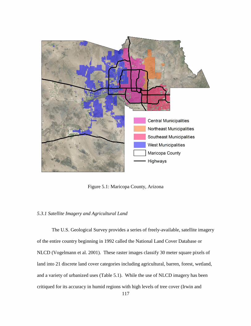
117
Figure 5.1: Maricopa County, Arizona
5.3.1 Satellite Imagery and Agricultural Land
The U.S. Geological Survey provides a series of freely-available, satellite imagery
of the entire country beginning in 1992 called the National Land Cover Database or
NLCD (Vogelmann et al. 2001). These raster images classify 30 meter square pixels of
land into 21 discrete land cover categories including agricultural, barren, forest, wetland,
and a variety of urbanized uses (Table 5.1). While the use of NLCD imagery has been
critiqued for its accuracy in humid regions with high levels of tree cover (Irwin and
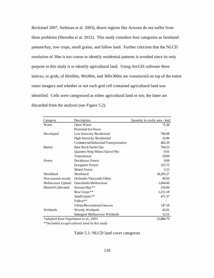
118
Bockstael 2007, Stehman et al. 2003), desert regions like Arizona do not suffer from
these problems (Shrestha et al. 2012). This study considers four categories as farmland:
pasture/hay, row crops, small grains, and fallow land. Further criticism that the NLCD
resolution of 30m is too coarse to identify residential patterns is avoided since its only
purpose in this study is to identify agricultural land. Using ArcGIS software three
lattices, or grids, of 60x60m, 90x90m, and 360x360m are constructed on top of the entire
raster imagery and whether or not each grid cell contained agricultural land was
identified. Cells were categorized as either agricultural land or not; the latter are
discarded from the analysis (see Figure 5.2).
Table 5.1: NLCD land cover categories
Category Description Quantity in study area - km2
Water Open Water 75.38
Perennial Ice/Snow -
Developed Low Intensity Residential 760.08
High Intensity Residential 14.96
Commercial/Industrial/Transportation 462.29
Barren Bare Rock/Sand/Clay 764.53
Quarries/Strip Mines/Gravel Pits 9.01
Transitional 19.09
Forest Deciduous Forest 9.09
Evergreen Forest 315.75
Mixed Forest 3.15
Shrubland Shrubland 18,293.27
Non-natural woody Orchards/Vineyards/Other 49.50
Herbaceous Upland Grasslands/Herbaceous 1,004.60
Planted/Cultivated Pasture/Hay** 216.84
Row Crops** 1,211.18
Small Grains** 471.37
Fallow** -
Urban/Recreational Grasses 147.19
Wetlands Woody Wetlands 45.01
Emergent Herbaceous Wetlands 12.51
*adapted from Vogelmann et al., 2001 23,884.79
**Included as agricultural land in this study
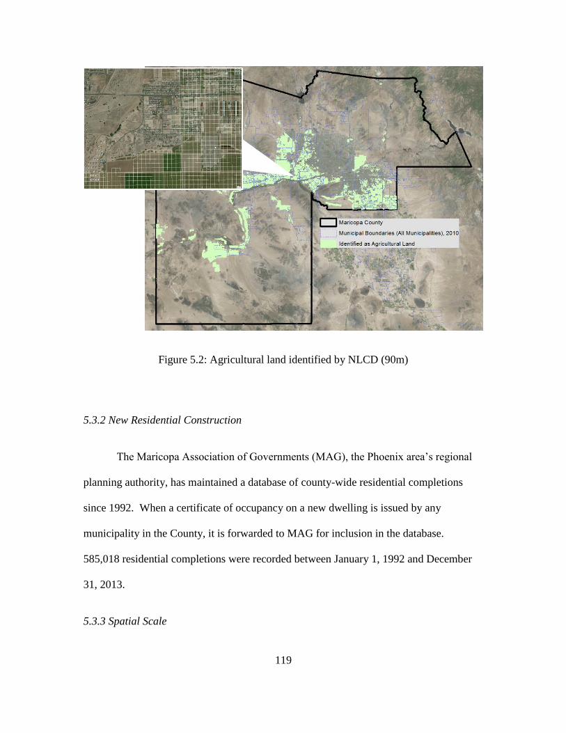
119
Figure 5.2: Agricultural land identified by NLCD (90m)
5.3.2 New Residential Construction
The Maricopa Association of Governments (MAG), the Phoenix area’s regional
planning authority, has maintained a database of county-wide residential completions
since 1992. When a certificate of occupancy on a new dwelling is issued by any
municipality in the County, it is forwarded to MAG for inclusion in the database.
585,018 residential completions were recorded between January 1, 1992 and December
31, 2013.
5.3.3 Spatial Scale
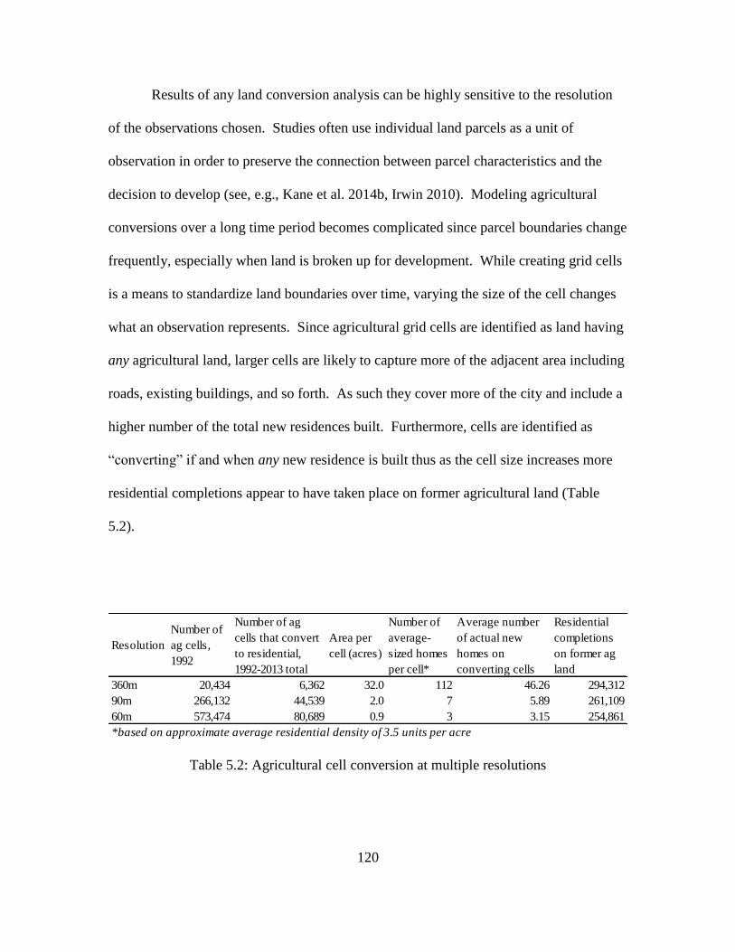
120
Results of any land conversion analysis can be highly sensitive to the resolution
of the observations chosen. Studies often use individual land parcels as a unit of
observation in order to preserve the connection between parcel characteristics and the
decision to develop (see, e.g., Kane et al. 2014b, Irwin 2010). Modeling agricultural
conversions over a long time period becomes complicated since parcel boundaries change
frequently, especially when land is broken up for development. While creating grid cells
is a means to standardize land boundaries over time, varying the size of the cell changes
what an observation represents. Since agricultural grid cells are identified as land having
any agricultural land, larger cells are likely to capture more of the adjacent area including
roads, existing buildings, and so forth. As such they cover more of the city and include a
higher number of the total new residences built. Furthermore, cells are identified as
“converting” if and when any new residence is built thus as the cell size increases more
residential completions appear to have taken place on former agricultural land (Table
5.2).
Table 5.2: Agricultural cell conversion at multiple resolutions
Resolution
Number of
ag cells,
1992
Number of ag
cells that convert
to residential,
1992-2013 total
Area per
cell (acres)
Number of
average-
sized homes
per cell*
Average number
of actual new
homes on
converting cells
Residential
completions
on former ag
land
360m 20,434 6,362 32.0 112 46.26 294,312
90m 266,132 44,539 2.0 7 5.89 261,109
60m 573,474 80,689 0.9 3 3.15 254,861
*based on approximate average residential density of 3.5 units per acre
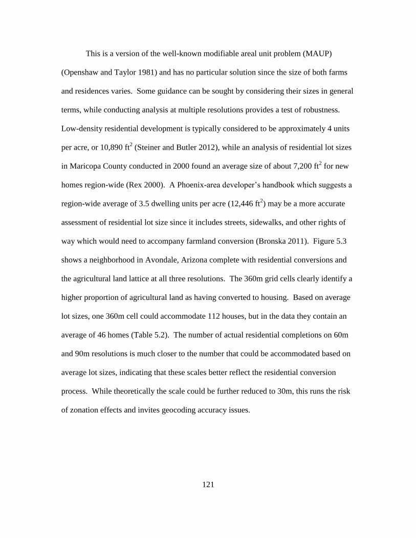
121
This is a version of the well-known modifiable areal unit problem (MAUP)
(Openshaw and Taylor 1981) and has no particular solution since the size of both farms
and residences varies. Some guidance can be sought by considering their sizes in general
terms, while conducting analysis at multiple resolutions provides a test of robustness.
Low-density residential development is typically considered to be approximately 4 units
per acre, or 10,890 ft2 (Steiner and Butler 2012), while an analysis of residential lot sizes
in Maricopa County conducted in 2000 found an average size of about 7,200 ft2 for new
homes region-wide (Rex 2000). A Phoenix-area developer’s handbook which suggests a
region-wide average of 3.5 dwelling units per acre (12,446 ft2) may be a more accurate
assessment of residential lot size since it includes streets, sidewalks, and other rights of
way which would need to accompany farmland conversion (Bronska 2011). Figure 5.3
shows a neighborhood in Avondale, Arizona complete with residential conversions and
the agricultural land lattice at all three resolutions. The 360m grid cells clearly identify a
higher proportion of agricultural land as having converted to housing. Based on average
lot sizes, one 360m cell could accommodate 112 houses, but in the data they contain an
average of 46 homes (Table 5.2). The number of actual residential completions on 60m
and 90m resolutions is much closer to the number that could be accommodated based on
average lot sizes, indicating that these scales better reflect the residential conversion
process. While theoretically the scale could be further reduced to 30m, this runs the risk
of zonation effects and invites geocoding accuracy issues.
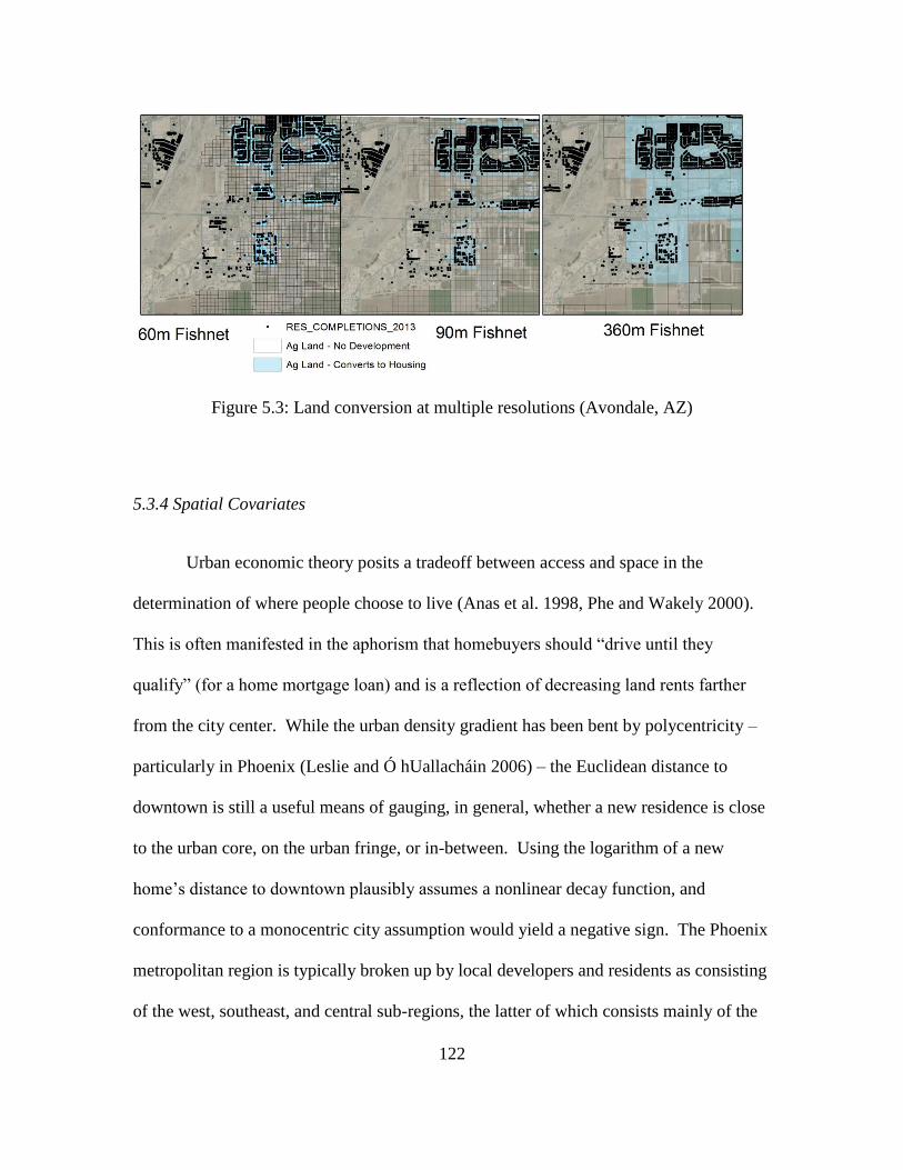
122
Figure 5.3: Land conversion at multiple resolutions (Avondale, AZ)
5.3.4 Spatial Covariates
Urban economic theory posits a tradeoff between access and space in the
determination of where people choose to live (Anas et al. 1998, Phe and Wakely 2000).
This is often manifested in the aphorism that homebuyers should “drive until they
qualify” (for a home mortgage loan) and is a reflection of decreasing land rents farther
from the city center. While the urban density gradient has been bent by polycentricity –
particularly in Phoenix (Leslie and Ó hUallacháin 2006) – the Euclidean distance to
downtown is still a useful means of gauging, in general, whether a new residence is close
to the urban core, on the urban fringe, or in-between. Using the logarithm of a new
home’s distance to downtown plausibly assumes a nonlinear decay function, and
conformance to a monocentric city assumption would yield a negative sign. The Phoenix
metropolitan region is typically broken up by local developers and residents as consisting
of the west, southeast, and central sub-regions, the latter of which consists mainly of the
123
city of Phoenix. A smaller northeast sub-region does not fit the typical descriptions and
mostly consists of the city of Scottsdale. Southeast, central, and northeast dummy
variables are considered relative to the reference category, west (see Figure 5.1).
Both agricultural rent and development costs are impacted by the soil quality.
Better soils require less maintenance and irrigation, lowering the cost per unit of farm
output. A contention of conservationists is often that prime agricultural lands are at the
highest risk of development, in particular since cities were originally formed in fertile
areas (Benfield et al. 2001). However this is largely an issue of perception since the price
of expensive farmland near urban areas is largely due to its exchange value, not
necessarily its agricultural productivity (Hart 2001). Since soil quality is a fairly static
characteristic of the land, this study relies on the U.S. Department of Agriculture’s most
recent soil survey as a covariate. Soil samples are digitized and were based on field
surveys conducted between 2010 and 2013 (NRCS, 2014b). The suitability of land for
agriculture is divided into four categories from best to worst: farmland of unique
importance, prime farmland if irrigated, prime farmland if irrigated and either protected
from flooding or not frequently flooded during the growing season, and not prime
farmland. A small area of Maricopa County is located in the Tonto National Forest for
which soil survey data is not available, though this land is left in the model for
completeness.
5.3.5 Institutional Covariates
During the study period highway construction was rapid: in 1992, Maricopa
County had 265 miles of limited-access freeways; a combination of interstate highways,
124
federal, and state roads. By 2013, this had increased to 461 miles (author’s calculation).
Freeway access is considered extremely important to real estate development generally,
and in Phoenix in particular (Tian and Wu 2015). Induced development has always been
a concern with respect to freeways, as plans for freeways lead to more building that is
increasingly dependent on freeway access (Kamel 2014). In order to account for the
changing freeway map over our study-period, a time-varying covariate Hwymiles is
added and is the Euclidean distance from the cell to the nearest highway that had been
built by that year. The anticipated negative coefficient would indicate that proximity to a
freeway increases the likelihood of development.
While zoning designation is typically considered in models of urban land-use
change, the ease of changing agricultural zoning to some other category in Maricopa
County means that its impact on housing construction is lessened (personal
communication with a former Phoenix city planner, October 2014). Kane et al. (2014c)
find mixed results regarding zoning before and during the recent recession, though the
relationship between land use and zoning became noticeably less concordant following
2006. Most municipalities in the region pursued an aggressive growth strategy that
involved annexing adjacent unincorporated lands, often sparring with one another in an
attempt to avoid being hemmed in and excluded from future growth opportunities (Heim
2012). This study considers both whether a grid cell was incorporated at the time of its
conversion, and if so, how long since it had become part of a municipality. Whether or
not land is incorporated is a rough indicator for the existence of city services and other
factors that could increase the likelihood or speed with which agricultural land is
converted to housing. However, it is likely that land annexation and development operate
125
hand-in-hand: the plans for a new residential development are likely to involve
discussions and action regarding its potential inclusion in a municipality. Since this may
result in an endogenous regressor, we also include the length of time between annexation
and land conversion as a covariate, i.e. are more recently annexed areas more likely to
convert? A negative coefficient would provide some evidence for endogeneity. It is also
possible to test the contention that construction on recently annexed land is more
prevalent during booms using an interaction term. In other words, is there a joint positive
effect of the recentness of annexation and high home prices?
5.3.6 Housing Market
An advantage of survival analysis in land-use change modeling is that spatially
and temporally-varying covariates can be compared. As shown in equation (1), a
landowner’s decision to convert land is a maximization of the present value of profit from
housing versus farming. This study uses the All-Transactions House Price Index for the
Phoenix-Mesa-Glendale, Arizona metropolitan statistical area (MSA) provided by the
Federal Reserve Bank of St. Louis to measure the variation in housing market conditions
over the study period (FRED 2014). While the potential profit from land conversion
necessarily involves myriad other factors that vary at a finer spatial scale, the land’s
location, accessibility, and municipal inclusion are already included separate which helps
to avoid endogeneity between these covariates and individual land prices. A positive sign
is expected, i.e. a higher housing price index will increase the hazard of land conversion.
A possible complication is that housing construction is not instantaneous: the decision to
develop is a reaction to current market conditions, while these data record land change

126
once homes are fully built. To account for the difference in time between the decision to
develop and the point in time at which land conversion is complete, we compare the
marginal effect of same-year price indices with prior-year indices and values for two
years prior. All price indices used in this study were inflation-adjusted using the
producer price index (PPI).
5.3.7 Agricultural Commodities Market and Oil Prices
Commodity crops have been a part of the Phoenix area’s economy since it was
first settled in the 1860s. Two of the most prevalent in the arid desert region are cotton
and alfalfa hay. In order to characterize the value of surviving (i.e. remaining as
farmland), this study considers the variation of the price index of these two crops over the
study period. The global index of cotton price is provided by the National Cotton
Council (2014a) and provides a measure of Phoenix-area crop in a global market.
Arizona alfalfa hay prices are acquired from the U.S. Department of Agriculture and
reflect a regional market feed crop (USDA 2014). Real crude oil prices are often used as
an indicator of the input price to farm production, as they are a component of both fuel
for machinery and a component of fertilizers. However, oil prices have a more complex
relationship with other economic measures. While low oil prices are often a bellwether
for economic conditions and are associated with higher U.S. stock market prices, oil
prices are endogenous to many components of the economy and the response of stock,
capital, or housing markets may depend on what caused the change in oil price (Kilian
and Park 2009). A negative coefficient would suggest they are more important for
127
homebuyers than for farmers, i.e. higher oil prices decrease consumers’ ability to
purchase new homes and therefore decrease the hazard of land conversion.
An additional hypothesis using an interaction term can investigate to what extent
oil prices correlate to where along the urban density gradient land will convert to
housing. Agricultural land is not unique to the urban fringe in the Phoenix area – since
the location of farms initially depended on water availability, many still exist in fairly
central parts of the region. We hypothesize that all else equal, residential conversions
will take place nearer the downtown when oil prices are high due to the increased cost of
intraurban transportation, while land conversion will favor the urban fringe when fuel
prices are lower. This hypothesis is supported by a number of studies suggesting that
higher fuel prices decrease various measures of urban sprawl. Dodson and Sipe (2007)
contend that more automobile-dependent urban areas in Australia are disproportionately
affected by rising fuel prices, while McGibany (2004) shows that U.S. metro areas with
higher gasoline prices tend to have smaller urban footprints. Measuring Canadian cities,
Tanguay and Gingras (2012) find that increased fuel prices increase the population in the
city center while decreasing the proportion of low-density housing. Ortuño-Padilla and
Fernández-Aracil (2013) echo this finding in Spain by comparing the construction rate of
single-family homes versus apartments.
5.4 Results and Discussion
Survival curves are analyzed first (Figure 5.4) followed by a discussion of
functional form. The main effects variables are then discussed, comparing results across
three different spatial scales (Table 5.3). Temporal lag is then addressed (Table 5.4),
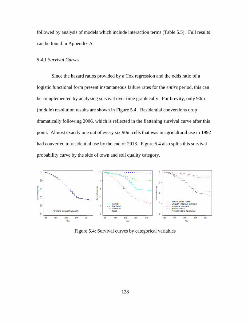
128
followed by analysis of models which include interaction terms (Table 5.5). Full results
can be found in Appendix A.
5.4.1 Survival Curves
Since the hazard ratios provided by a Cox regression and the odds ratio of a
logistic functional form present instantaneous failure rates for the entire period, this can
be complemented by analyzing survival over time graphically. For brevity, only 90m
(middle) resolution results are shown in Figure 5.4. Residential conversions drop
dramatically following 2006, which is reflected in the flattening survival curve after this
point. Almost exactly one out of every six 90m cells that was in agricultural use in 1992
had converted to residential use by the end of 2013. Figure 5.4 also splits this survival
probability curve by the side of town and soil quality category.
Figure 5.4: Survival curves by categorical variables
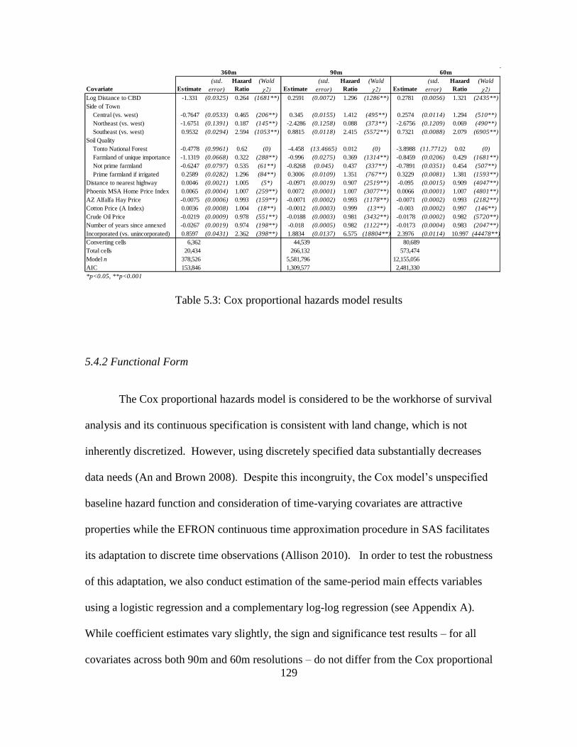
129
Table 5.3: Cox proportional hazards model results
5.4.2 Functional Form
The Cox proportional hazards model is considered to be the workhorse of survival
analysis and its continuous specification is consistent with land change, which is not
inherently discretized. However, using discretely specified data substantially decreases
data needs (An and Brown 2008). Despite this incongruity, the Cox model’s unspecified
baseline hazard function and consideration of time-varying covariates are attractive
properties while the EFRON continuous time approximation procedure in SAS facilitates
its adaptation to discrete time observations (Allison 2010). In order to test the robustness
of this adaptation, we also conduct estimation of the same-period main effects variables
using a logistic regression and a complementary log-log regression (see Appendix A).
While coefficient estimates vary slightly, the sign and significance test results – for all
covariates across both 90m and 60m resolutions – do not differ from the Cox proportional
Covariate Estimate
(std.
error)
Hazard
Ratio
(Wald
χ2) Estimate
(std.
error)
Hazard
Ratio
(Wald
χ2) Estimate
(std.
error)
Hazard
Ratio
(Wald
χ2)
Log Distance to CBD -1.331 (0.0325) 0.264 (1681**) 0.2591 (0.0072) 1.296 (1286**) 0.2781 (0.0056) 1.321 (2435**)
Side of Town
Central (vs. west) -0.7647 (0.0533) 0.465 (206**) 0.345 (0.0155) 1.412 (495**) 0.2574 (0.0114) 1.294 (510**)
Northeast (vs. west) -1.6751 (0.1391) 0.187 (145**) -2.4286 (0.1258) 0.088 (373**) -2.6756 (0.1209) 0.069 (490**)
Southeast (vs. west) 0.9532 (0.0294) 2.594 (1053**) 0.8815 (0.0118) 2.415 (5572**) 0.7321 (0.0088) 2.079 (6905**)
Soil Quality
Tonto National Forest -0.4778 (0.9961) 0.62 (0) -4.458 (13.4665) 0.012 (0) -3.8988 (11.7712) 0.02 (0)
Farmland of unique importance -1.1319 (0.0668) 0.322 (288**) -0.996 (0.0275) 0.369 (1314**) -0.8459 (0.0206) 0.429 (1681**)
Not prime farmland -0.6247 (0.0797) 0.535 (61**) -0.8268 (0.045) 0.437 (337**) -0.7891 (0.0351) 0.454 (507**)
Prime farmland if irrigated 0.2589 (0.0282) 1.296 (84**) 0.3006 (0.0109) 1.351 (767**) 0.3229 (0.0081) 1.381 (1593**)
Distance to nearest highway 0.0046 (0.0021) 1.005 (5*) -0.0971 (0.0019) 0.907 (2519**) -0.095 (0.0015) 0.909 (4047**)
Phoenix MSA Home Price Index 0.0065 (0.0004) 1.007 (259**) 0.0072 (0.0001) 1.007 (3077**) 0.0066 (0.0001) 1.007 (4801**)
AZ Alfalfa Hay Price -0.0075 (0.0006) 0.993 (159**) -0.0071 (0.0002) 0.993 (1178**) -0.0071 (0.0002) 0.993 (2182**)
Cotton Price (A Index) 0.0036 (0.0008) 1.004 (18**) -0.0012 (0.0003) 0.999 (13**) -0.003 (0.0002) 0.997 (146**)
Crude Oil Price -0.0219 (0.0009) 0.978 (551**) -0.0188 (0.0003) 0.981 (3432**) -0.0178 (0.0002) 0.982 (5720**)
Number of years since annexed -0.0267 (0.0019) 0.974 (198**) -0.018 (0.0005) 0.982 (1122**) -0.0173 (0.0004) 0.983 (2047**)
Incorporated (vs. unincorporated) 0.8597 (0.0431) 2.362 (398**) 1.8834 (0.0137) 6.575 (18804**) 2.3976 (0.0114) 10.997 (44478**)
Converting cells 6,362 44,539 80,689
Total cells 20,434 266,132 573,474
Model n 378,526 5,581,796 12,155,056
AIC 153,846 1,309,577 2,481,330
*p<0.05, **p<0.001
360m 90m 60m
130
hazards modeli. Therefore the remainder of discussion will focus exclusively on Cox
model results.
5.4.3 Cox Proportional Hazards Model Results
A first glance at parameter estimates and their associated hazard ratios in Table
5.3 indicates first that, no matter the scale, chi-squared values are high and nearly all
variables are significant – regardless of spatial scale. This is simply a result of the high
number of observations in the model. Due to the use of time-varying covariates, each
cell is observed each year until it converts. For the 60m resolution models, 573,474
agricultural cells results in 12,155,056 observations in the regression. The Akaike
Information Criterion (AIC) is used to compare across models (though, not across
resolutions); a lower value indicates a better overall fit. Results are reported and
discussed as hazard ratios, which indicate the covariate’s effect on an observation’s
relative failure rate over the entire study period, evaluated using a chi-squared test.
5.4.4 Main Effects – Spatial Covariates
The effect of distance to downtown on the hazard of conversion is strongly
negative at 360m resolution – an additional (log) mile from downtown decreases the
hazard of conversion by 73.6%. While this appears consistent with a monocentric city
assumption, it is largely an artifice of scale, as additional distance significantly increases
the hazard of conversion in the 90m and 60m models – by about 30% per log mile.
Outlying areas are more likely to convert. Scale-sensitivity is seen in the side-of-town
variables as well: while these have some of the highest chi-squared values across all
131
covariates, signs differ between coarse and finer resolutions. At 360m resolution, the
hazard of conversion is highest for agricultural land in the southeast valley, followed by
west, central, then northeast. While the southeast valley maintains the highest hazard of
conversion at the finer resolutions (see Figure 5.4), the central area – consisting
principally of the city of Phoenix – has a higher hazard of conversion than the west valley
in these models. This can be attributed to the characteristics the city of Phoenix’s
farmland, which generally consisted of smaller farms whose size was less attractive to
developers until the late boom period of the early 2000s. These developments were also
less attractive to develop until later (despite their close proximity due to downtown)
because they are in the Hispanic-majority neighborhood of South Phoenix (Kane et al.
2014c). Since these results demonstrate that 360m resolution is too coarse to pick up
certain types of agricultural land in the region, subsequent interpretation of results will
focus on the 90m and 60m models.
The contention that urbanization is most prevalent on the best farmland is not
supported (see Figure 5.4). Farmland of unique importance has a 57% to 63% lower
hazard of conversion than the third-best category which is farmland that is irrigated and
flood-protected. The second-best soil – prime farmland that is irrigated but does not
require flood protection – demonstrates the highest hazard of conversion to residential
use. In fact, nonprime farmland and farmland of unique importance have fairly similar
hazard ratios. This likely reflects the delineation of soil quality categories by the USDA,
which defines farmland of unique importance region-by-region and includes specific
high-value crops. The distinction that is more important may lie in the difference
between development on agricultural land versus open desert. Following the state’s
132
1980 Groundwater Management Act, a developer must demonstrate a 100-year supply of
water before proceeding. This is easy on agricultural land which necessarily has existing
water rights, though development on previously unoccupied desert requires a more
difficult and expensive process to meet this requirement (Staudenmaier 2007).
5.4.5 Main Effects – Institutional Covariates
The effect of distance to the nearest limited-access freeway is a time-varying
covariate since only 57% of the present-day freeway miles in the region had been built by
1992. The negative coefficient indicates that each additional mile from an existing
freeway decreases the hazard of conversion by about 9%. Proximity to the transportation
network is a positive attribute for new housing rather than a negative externality. This
covariate’s explanatory power is higher than that for the distance to the downtown area,
which might be expected in a polycentric region like Phoenix. There may be somewhat
of a concern over the endogeneity of freeway proximity to land conversion since this
study considers distance to the nearest freeway that had already been built at the time in
question. However, freeways are not necessarily built to serve existing population –
developers are likely to acquire property and begin the process of homebuilding based on
the expectation of future freeway construction. Since most area freeways were planned
by the Arizona Department of Transportation in their original 1985 regional plan (2010),
the point at which a developer realistically believes a highway will be built in time to
serve newly-built housing is not entirely clear. As such, the question of the inductive,
pre-construction effects of highway planning remains unexplored in this study.
133
The Phoenix area has a long history of competitive land annexation (Heim 2012).
Results show that whether an agricultural parcel is within municipal boundaries is by far
the strongest contributor to its hazard of conversion, ranging between a 657% to a 1099%
increase in hazard ratio based on this covariate. However, the number of years elapsed
since land was first included within municipal borders has a negative effect on the hazard
ratio: an additional year elapsed since annexation reduced the hazard of conversion by
1.7% to 1.8%. In other words, newly annexed farmland is more likely to develop,
suggesting that the processes of annexation and development go hand-in-hand as land
developers negotiate with municipalities for inclusion and housing is quickly built. While
the magnitude of this effect is smaller and likely varies from case to case, it clearly
indicates that newly annexed land is seen more favorably for development. This is
consistent with historical narratives of Phoenix which stress the importance of greenfield
development and overall newness (Gober 2006) while highlighting the difficulty of infill
growth in the region’s core areas. In other words, older land becomes less desirable to
convert.
5.4.6 – Main Effects – Market-Based Covariates
Interpretation of the hazard ratio of the price indices used in this study is
straightforward and reflects the impact on conversion hazard of a one percentage point
change in the indexed value. As expected, the metropolitan-level home price index has a
positive and significant impact on the hazard of conversion. While its explanatory power
(χ2) is lower than some other covariates, it is consistent across all three resolutions: a one
percentage point increase in home-price index increases the hazard of conversion by
134
0.7%. Conversely, and consistent with our hypothesis, an increase in cotton and alfalfa
hay prices each decrease the hazard of conversion. A one percentage point increase in
the regional price of alfalfa hay decreases conversion hazard by 0.7%. The relationship
between cotton prices, which is traded on a global market, and conversion hazard
operates in the same direction but is far weaker; a one percentage point increase
decreases conversion hazard by 0.1% to 0.3%.
The relationship between crude oil price and conversion hazard was hypothesized
to operate in two directions: positively as an agricultural input and negatively as a
component of consumer/homebuyer spending. Oil price has a strong, negative
coefficient – a one percentage point increase decreases the hazard of conversion by
between 1.8% and 2.2% - the most of any price variable. This supports the hypothesis
that oil price negatively impacts new housing development more than it increases a
farmer’s costs such that he is motivated to sell his land. Conversion hazard clearly
decreases when oil prices are high.
5.4.7 – Lagged Main Effects
This study’s dependent variable of land conversion is measured by the date on
which a certificate of occupancy was granted for a new residence. While the decision to
develop land must take place prior to this, how long before is unclear. A study of
Michigan homebuilders suggested an average of eighteen months from development
conception to completion (Vigmostad 2003). Given Arizona’s year-round construction
season and the rapid pace of Sunbelt housing growth during boom periods, this figure
could be far lower locally.
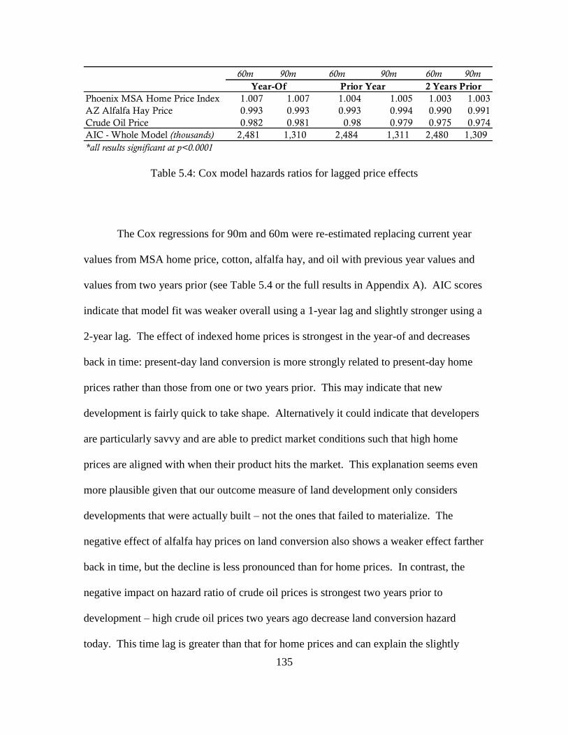
135
Table 5.4: Cox model hazards ratios for lagged price effects
The Cox regressions for 90m and 60m were re-estimated replacing current year
values from MSA home price, cotton, alfalfa hay, and oil with previous year values and
values from two years prior (see Table 5.4 or the full results in Appendix A). AIC scores
indicate that model fit was weaker overall using a 1-year lag and slightly stronger using a
2-year lag. The effect of indexed home prices is strongest in the year-of and decreases
back in time: present-day land conversion is more strongly related to present-day home
prices rather than those from one or two years prior. This may indicate that new
development is fairly quick to take shape. Alternatively it could indicate that developers
are particularly savvy and are able to predict market conditions such that high home
prices are aligned with when their product hits the market. This explanation seems even
more plausible given that our outcome measure of land development only considers
developments that were actually built – not the ones that failed to materialize. The
negative effect of alfalfa hay prices on land conversion also shows a weaker effect farther
back in time, but the decline is less pronounced than for home prices. In contrast, the
negative impact on hazard ratio of crude oil prices is strongest two years prior to
development – high crude oil prices two years ago decrease land conversion hazard
today. This time lag is greater than that for home prices and can explain the slightly
60m 90m 60m 90m 60m 90m
Phoenix MSA Home Price Index 1.007 1.007 1.004 1.005 1.003 1.003
AZ Alfalfa Hay Price 0.993 0.993 0.993 0.994 0.990 0.991
Crude Oil Price 0.982 0.981 0.98 0.979 0.975 0.974
AIC - Whole Model (thousands) 2,481 1,310 2,484 1,311 2,480 1,309
*all results significant at p<0.0001
Year-Of Prior Year 2 Years Prior
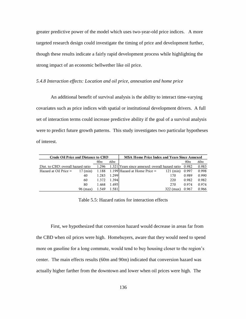
136
greater predictive power of the model which uses two-year-old price indices. A more
targeted research design could investigate the timing of price and development further,
though these results indicate a fairly rapid development process while highlighting the
strong impact of an economic bellwether like oil price.
5.4.8 Interaction effects: Location and oil price, annexation and home price
An additional benefit of survival analysis is the ability to interact time-varying
covariates such as price indices with spatial or institutional development drivers. A full
set of interaction terms could increase predictive ability if the goal of a survival analysis
were to predict future growth patterns. This study investigates two particular hypotheses
of interest.
Table 5.5: Hazard ratios for interaction effects
First, we hypothesized that conversion hazard would decrease in areas far from
the CBD when oil prices were high. Homebuyers, aware that they would need to spend
more on gasoline for a long commute, would tend to buy housing closer to the region’s
center. The main effects results (60m and 90m) indicated that conversion hazard was
actually higher farther from the downtown and lower when oil prices were high. The
90m 60m 90m 60m
Dist. to CBD: overall hazard ratio 1.296 1.321 Years since annexed: overall hazard ratio 0.982 0.983
Hazard at Oil Price = 17 (min) 1.188 1.199 Hazard at Home Price = 121 (min) 0.997 0.998
40 1.283 1.299 170 0.989 0.990
60 1.372 1.394 220 0.982 0.982
80 1.468 1.495 270 0.974 0.974
96 (max) 1.549 1.581 322 (max) 0.967 0.966
Crude Oil Price and Distance to CBD MSA Home Price Index and Years Since Annexed
137
coefficient of the interaction term, 𝛽1,2 (the joint coefficient estimate of two covariates,
i.e. 𝛽1,2𝑋1𝑋2) is positive in both 90m and 60m models indicating reinforcing effects;
however, the effects were not in the expected direction. Table 5.5 displays the overall
hazard ratio of the distance to downtown variable along with the hazard ratio at a variety
of different oil prices, calculated from 𝛽1,2. As oil prices increase so does the hazard
ratio for distance: high fuel prices actually increase the hazard of conversion of land
farther from the city center. This is contrary to our transportation cost hypothesis and
may represent a substitution effect: high gasoline prices decrease income, leaving
homebuyers to search for cheaper housing at the urban fringe. While this would seem to
increase transportation costs, it may not matter much for some: fringe homebuyers may
be retirees who don’t commute, they may also work in that part of the region, or they
may be lower-income individuals don’t have the credit needed to finance a bigger
mortgage but can fairly easily spend more at the gas pump. Furthermore, destinations
like shopping, employment, and recreation may be so concentrated in urban subcenters
that the relationship between a residence and the region’s core area is no longer
important. This result contrasts with previous findings relating fuel price to urban form,
which have varied in their outcome measure. While this study’s use of Euclidean
distance to downtown could be more nuanced with respect to polycentricity and an
outcome metric of agricultural conversion omits other types of development, it does
improve on previous work by examining within-city development decisions over a time
horizon which saw drastic changes in oil price. Though this finding is reflective of the
Phoenix area, its clarity and strength demonstrate that the perspective that higher oil
prices will result in compact cities is far from a universal truth.
138
We also hypothesized that in booming times when home prices were high
conversion hazard will increase on land that was recently annexed into a municipality.
This would provide further evidence of endogeneity between annexation and
development. The main effects result indicated that more elapsed time between
annexation and land conversion decreases the hazard of conversion. Taking home prices
into consideration, this effect is magnified: during housing price booms, the hazard of
conversion based on elapsed time decreases, i.e. newly annexed land is more at risk. This
provides further evidence that in booming times development is on even more recently
annexed land, consistent with historical narratives of Phoenix.
5.5 Conclusions
This study investigates the conversion of agricultural land in the Phoenix
metropolitan area from 1992 to 2013 using survival analysis. A variety of conclusions
emerge about land conversion in Phoenix, the practice of modeling urban land-use
change, and urban morphology more generally.
The Phoenix area is emblematic of fast-growing regions in the American Sunbelt,
and some of its eccentricities are uncovered in this study. There is clearly no “death of
Geography;” agricultural land that is farther out from the city center but with good
highway access is at the highest risk of conversion. The Southeast subregion dominates,
while the best soils are not necessarily at higher risk of conversion. Farmland within
municipal boundaries – and in particular farmland that has recently been annexed into
municipalities has an increased hazard of converting. This is consistent with the region’s
emphasis on newness and its history of competitive land consumption – by homebuyers
139
and also municipalities in their desire to annex land. Evidence does suggest that
development and annexation operate together – particularly during booms.
While much of this study’s research design was tailored to the case of agricultural
land in central Arizona, it demonstrates the usefulness of survival analysis in
understanding urban growth and the benefits of including varying market conditions (in
this case, both regional and global) into spatially-explicit modeling of land-use change.
Future applications can focus on urban growth simulation and more targeted scenario
planning. Predicting the impact of new highway construction, development impact fees,
urban growth restrictions, or zoning alternatives on the hazard of land conversion could
be easily handled using a Monte Carlo approach. While more complex land-use change
platforms like UrbanSim are well-established and consist of many interacting sub-
models, binary or multinomial outcome studies like this should be seen as a lightweight
complement. However, they must be designed carefully. While this study did not find
variation in results based on alternative functional forms, both spatial and temporal
resolution impacted the results and must be chosen meticulously.
This study began with the fairly apparent hypothesis that varying market
conditions have a large role in land conversion and urban morphological change.
Empirical results confirm: while a number of factors show high statistical power,
economic indicators – particularly the expected return on metro-level home construction
and oil prices, an economic bellwether, are equally if not more important than spatial and
institutional drivers of land development. Contrasting the strong effect of same-period
housing prices with the lagged impact of oil prices on development highlights the
difference between a global bellwether and the uniqueness of the process of land
140
development, which may be fairly quick to take shape or speculative in nature. More
generally it demonstrates the reach of global economic forces on land change decisions.
Future research on urban land-use change should strive to include market indicators –
including both those related to the housing industry such as home mortgage rates but also
other national and global financial indicators. The recent global financial crisis
demonstrated, rather starkly, the upward and downward connections between local
markets for space and global markets for financial capital (Martin 2010).
Additionally, trends in cities such as preference for compact growth or fringe
development should be researched thoroughly, positively, and across a wide variety of
regions. The seemingly logical understanding that an increase in transportation costs will
result in either compact growth or less fringe development is clearly incomplete. This
study demonstrates that in a region characterized by fast growth and fairly cheap housing,
higher oil prices could induce a substitution effect whereby new land is developed even
farther toward the urban fringe. This has implications for understanding the role of
proximity to a city center, which for retirees or suburban employees might mean very
little. It also has implications for social equity: the ability for an individual to substitute
transportation expense for housing expense is limited by access to credit. Finally, given
concerns over the sustainability of Greenfield development and the policy interest in
promoting compact growth and infill development, this study highlights the importance
of understanding that developers’ and homebuyers’ response to market conditions, when
measured in land-use changes, may not be as expected. This is a key finding for anyone
interested in urban morphological change.
141
CHAPTER 6
CONCLUSIONS
This dissertation uses four individual research studies to investigate the historic,
geographic microfoundations of Phoenix’s urban morphology and the drivers of land
development behind it. This conclusion first recapitulates the specific findings from
these research studies then provides a discussion of their implications for urban research
and urban theory. Finally, specific policy recommendations are considered.
6.1 Key Findings
Chapter 1 investigated how land-use heterogeneity and complementarity
developed in historic Phoenix. The exodus from downtown following World War II was
more closely related to residential parcels than retail decline, which is a commonly held
contention of critics of today’s high levels of vacancy in downtown Phoenix. This
supports Sternleib’s (prescient) 1963 contention that residential suburbanization isolated
downtown retail which itself languished. Continual homogenization by land-use type is
found to exist during this period as well; Phoenix did become more ordered from 1915-
1963. Rather than wholesale land-use incompatibility, negative externalities were likely
restricted to certain neighborhoods that remained near concentrating industrial land uses.
Chapter 2 studies the meaning of fragmentation in discussions of urban sprawl,
investigating land cover in Phoenix’s census block groups based on when present-day
structures were built. Observing within-lot rather than between-lot variation, newer-
developing areas (which are not necessarily farther from the CBD) are less diverse and
more homogenous in terms of land cover, reflecting the recent trend toward xeric
landscaping and larger, more complex development styles that actually involve fewer
142
cover types. In other words, areas developed since the 1990s are both more fragmented
and more homogenous, though their landscaping may be more congruous with the
surrounding desert ecosystem.
In comparing time periods directly before and after the global financial crisis of
the late 2000s, Chapter 4 finds that boom-period housing was characterized by lower-
cost, lower-density development on converted farmland in the interstices between
regional subcenters. Following the collapse, development was more likely to be transit-
adjacent, near commercial uses and public parks, on higher-valued land with higher-
valued neighbors. This reflects a combination of evolving preferences for housing and
changes in how housing is treated in the broader asset market. Some have termed this an
“urban inversion” (Ehrenhalt 2012, Leinberger 2011, Plane 2013). Chapter 5 confirms
the strong role of housing and agricultural market conditions in land conversion over a
broader temporal and spatial extent, finding endogeneity in the relationship between
municipal annexation and development and a strong role for oil prices in determining
land development along an urban density gradient.
6.2 Implications for Urban Research and Urban Theory
This dissertation’s chapters provide an implicit comparison of different spatial
conceptions of a city. While Chapter 2 only covers a small fraction of present-day
Phoenix, its rapid decline following World War II had long-lasting implications for the
downtown core. Chapter 3 found so few block groups developed prior to the 1940s that
empirical comparison with newer regions wasn’t practical, highlighting the difficulty in
drawing boundaries for space-time analysis. While Chapter 4 analyzes the municipality
of Phoenix as a case study, analysis is best done on the level of a metropolitan area when
143
possible – such as in Chapter 5 – as it represents a functional labor market area instead of
a potentially arbitrary metropolitan border.
Phoenix’s well-known polycentricity continually presents itself in this
dissertation. Chapter 3 argues that development timing is more relevant than Euclidean
distance for understanding land cover differentiation. However, Chapters 4 and 5 note
that development based on distance to downtown is heavily scale-sensitive given the
differences in parcel sizes across the region. While the fine-resolution results in Chapter
5 indicate that agricultural conversion (1992-2013) is more likely farther from the city
center, Chapter 4 found evidence in more recent periods (2002-2006, 2006-2012) that
either proximity or greater distance could be preferred. A more exhaustive study of
commuter and household activity patterns – perhaps based on travel surveys or commute
data – could relate a more nuanced concept of proximity to land-use change.
The practices of choosing an appropriate urban extent and conceptualizing
intraurban location stress the need for local geographic knowledge even in quantitative
analysis. Interpreting results and making decisions in processing fine-scaled geographic
data could induce bias without at least some familiarity with the peculiarities of a region.
This problem complicates interurban analysis of within-city patterns, as demonstrated by
the resolution and spatial metric-induced systematic bias found in Burchfield et al.’s
(2006) nationwide analysis of urban sprawl (Irwin and Bockstael 2007). Comparative
studies involving several local experts such as York et al.’s (2011a) study of land
fragmentation in five cities represent a partial solution. The increasing availability of
parcel-level data from municipal governments and planning agencies provides consistent,
fine-resolution information that can be compared across several regions at a time, though
144
local history, physical topography, cross-municipal differences, and many other factors
complicate even simple decisions like the delineation of space and time. Mirroring the
spatial and temporal data-generating processes as well as using parcel-level data (Irwin
2010) are high on a list of best practices.
While this complicates empirical analysis, a theoretical hurdle to overcome is the
over-reliance on the term “urban sprawl.” Popularized in part by groups like the National
Resources Defense Council (Benfield et al. 2001), the term is intended to summarize a
number of concerns over urban morphology but lacks specificity and objectivity. In
particular, Chapter 3 makes clear that the concepts of sprawl and fragmentation vary
based on data resolution. Instead, focus should be placed on sprawl’s constituent parts
(see, e.g., Brueckner 2000) such as transportation, energy consumption, municipal
infrastructure provision, landscape cover, and land use complementarity. A bricolage
approach, such as Sampson’s (2013) Project on Human Development in Chicago
Neighborhoods or this dissertation on metropolitan Phoenix combines many related
outcome measures in a particular region and combines empirical analysis with local
geographic knowledge. The recent accumulation of academic publications on urban
Phoenix has led to the informal creation of a desert school of urbanism which prioritizes
sustainability in a fast-growing yet ecologically-fragile metropolis, analyzing land cover
(e.g. Connors et al. 2012), environmental justice (e.g. Bolin et al. 2005), urban
morphology (e.g. Gober and Burns 2002) and other outcome measures through a variety
of social and physical science approaches.
A final, related component to local knowledge stressed throughout this
dissertation is the importance of path-dependence and historical legacies in the creation
145
of current and future urban spaces. This is seen in the variety of findings which relate
land change and distance to downtown, and also the significant differences in land cover
by development timing found in Chapter 3. Despite recent development in downtown
Phoenix, its oversupply of vacant land and surface parking today are legacies of the
postwar decline examined in Chapter 2. Municipal incorporation and the region’s
“annexation wars,” which in Chapter 5 have a greater impact on agricultural land
conversion than anything else, demonstrate that historical legacies can be institutionally
as well as market-shaped.
Future work on methodological advancement should focus on validation of
geographic statistical measures, policy counterfactuals, and a wider array of econometric
outcome measures. While Chapter 2 uses random permutations to assess the significance
of join-counts and land use transitions, assessing measures on simulated data could allay
concerns over the reliability of results, especially across different regions. Studies such
as Rey and Folch (2011) demonstrate this for particular indexed values. Chapters 4 and 5
use a binary dependent variable of developed versus undeveloped to investigate drivers of
land change. As such Chapter 4’s scope is limited to conclusions about single-family
housing and Chapter 5’s is limited to development on agricultural land. While this
particular transition type is very prevalent in the study region, a multinomial approach
like that of Levine (1998) is an extension that could simultaneously investigate multiple
land change outcomes (single-family versus multifamily versus commercial, for example)
while increasing predictive power. Inclusion of a mechanism for land prices (e.g., Wrenn
and Irwin 2012) or a hedonic approach such as Golub et al. (2012) which uses home sales
as a dependent variable can be a component of or a complement to the binary outcome
146
metrics used in Chapters 4 and 5. A particularly attractive extension is the construction
of policy counterfactuals, e.g., predicting the land development impact of a proposed new
highway, development impact fees, or a zoning change. While UrbanSim and other
coupled land use-transportation models are powerful and well-established (Waddell
2000), studies using a Cox regression plus a Monte Carlo simulation are highly adaptable
and can be made lightweight enough to predict ranges and confidence intervals.
6.3 Policy Recommendations
The methods used in this dissertation hold high promise for future work that is
more specifically tailored toward policy proposals, though a number of recommendations
can be made based on these results. Chapter 4’s findings on South Phoenix emphasize
potential equity concerns surrounding land-use change and also provide some evidence of
changing tastes such as nearby transit and public parks. The former should be scrutinized
and the latter should be encouraged by favorable and unencumbered zoning designations
that promote types of development that area residents increasingly desire. If market
forces are sufficient to promote compact or infill growth, policy intervention in the form
of subsidies may not be needed though it could help overcome encumbrances to
investment in certain locations. Incentives, though, should be tailored toward public
improvements rather than subsidizing development outright (Kane and Weber In
Revision).
Chapter 5’s findings are less optimistic though they do hint at a potential for
successful intervention. A continual preference for land conversion in newly-annexed
areas is inconsistent with compact growth objectives and indicates that Greenfield
development may be disproportionately unencumbered, profitable, or actively promoted
147
by municipal governments. Intervention such as transit-oriented zoning or credits for
adaptive re-use of previously developed land could direct development capital toward
areas with existing infrastructure and lower transportation costs while preserving
agricultural or natural lands. Recent evidence suggests some of these efforts, at least in
the Phoenix area, might be effective (Golub et al. 2012).
A counterintuitive finding from Chapter 5 is that land conversion hazard increases
with distance from the downtown in times of high oil prices. While this merits further
investigation using a more targeted research design, this finding should be a signal to
policymakers that substitution of transportation expense for more accessible housing is
not a given, particularly since this substitution would be more difficult for lower-income
households. Especially as the “Fordist-era” suburban-style housing stock ages and
decreases in price (Kamel 2014), its location relative to employment, shopping, and
recreation needs to be considered by researchers and homebuyers alike as it could very
well lead to increased transportation need despite higher fuel costs. This also supports
the rationale of location efficient mortgages (Blackman and Krupnick 2001), which seek
to facilitate the substitution of transportation cost with the (typically higher) cost of
housing that requires less transportation.
148
REFERENCES
2010. Maricopa County, Arizona: Regional transportation plan. The National Academies:
Transportation Research Board.
2012. Agricultural Property Manual. ed. P. T. Division. Phoenix, AZ: Arizona
Department of Revenue.
2013. The Zoning Ordinances of the City of Phoenix. In G-5777, ed. C. o. Phoenix.
Seattle, Washington: Code Publishing Company.
2014a. "A" Index. National Cotton Council of America.
2014b. National Resource Conservation Service Web Soil Survey. ed. U. S. D. o.
Agriculture. Washington, D.C.
Aalbers, M. B. (2009) The sociology and geography of mortgage markets: Reflections on
the financial crisis. International Journal of Urban and Regional Research, 33,
281-290.
Adams, J. S. (1970) Residential Structure of Midwestern Cities. Annals of the Association
of American Geographers, 60, 37-62.
Agarwal, S., B. W. Ambrose, S. Chomsisengphet & A. B. Sanders (2012) Thy Neighbor
’s Mortgage: Does Living in a Subprime Neighborhood Affect One’s
Probability of Default? Real Estate Economics, 40, 1-22.
Alberti, M. (2005) The effects of urban patterns on ecosystem function. International
Regional Science Review, 28, 168-192.
Alberti, M. & J. Marzluff (2004) Ecological resilience in urban ecosystems: linking urban
patterns to human and ecological functions. Urban Ecosystems, 7, 241-265.
Allison, P. 2010. Survival Analysis Using SAS. Cary, NC: SAS Institute.
Allison, P. D. 1999. Logistic Regression Using SAS: Theory and Application. Cary, North
Carolina: John Wiley & Sons.
Alonso, W. 1964. Location and Land Use: Toward a General Theory of Land Rent.
Cambridge: Harvard University Press.
An, L. & D. G. Brown (2008) Survival analysis in land change science: Integrating with
GIScience to address temporal complexities. Annals of the Association of
American Geographers, 98, 323-344.
149
Anas, A., R. Arnott & K. A. Small (1998) Urban spatial structure. Journal of Economic
Literature, 36, 1426-1464.
Arthur, W. B. 1988. Urban systems and historical path-dependence. In Cities and Their
Vital Systems, eds. J. Ausubel & R. Herman. Washington, D.C.: National
Academy Press.
Atkinson-Palombo, C. (2010) New housing construction in Phoenix: Evidence of "new
suburbanism"? Cities, 27, 77-86.
Baatz, M. & A. Schape (2000) Multiresolution segmentation: An optimization approach
for high quality multi-scale image segmentation. Angewandte geographische
informationsverarbeitung, 12, 12-23.
Banzhaf, E. & R. Hofer (2008) Monitoring Urban Structure Types as Spatial Indicators
With CIR Aerial Photographs for a More Effective Urban Environmental
Management. IEEE Journal of Selected Topics in Applied Earth Observations
and Remote Sensing, 1, 129-138.
Batty, M. 2005. Cities and Complexity: Understanding Cities with Cellular Automata,
Agent-Based Models, and Fractals. Cambridge, Mass.: MIT Press.
Bausch, J. C., H. Eakin, S. Smith-Heisters, A. M. York, D. D. White, C. Rubiños & R. M.
Aggarwal (2015) Development pathways at the agriculture–urban interface: the
case of Central Arizona. Agriculture and Human Values.
Bell, K. P. & E. G. Irwin (2002) Spatially explicit micro-level modelling of land use
change at the rural-urban interface. Agricultural Economics, 27, 217-232.
Bell, N., N. Schuurman & S. M. Hameed (2008) Are injuries spatially related? Join-count
spatial autocorrelation for small-area injury analysis. Injury Prevention, 14, 346-
353.
Benfield, F. K., M. D. Raimi & D. D. T. Chen. 2001. Once There Were Greenfields: How
Urban Sprawl is Undermining America's Environment, Economy, and Social
Fabric. New York: Natural Resources Defense Council.
Benz, U. C., P. Hofmann, G. Willhauck, I. Lingenfelder & M. Heynen (2004) Multi-
resolution, object-oriented fuzzy analysis of remote sensing data for GIS-ready
information. ISPRS Journal of Photogrammetry and Remote Sensing, 58, 239-
258.
Berke, P. R. (2002) Does Sustainable Development Offer a New Direction for Planning?
Challenges for the Twenty-First Century. Journal of Planning Literature, 17, 21-
36.
150
Blackman, A. & A. Krupnick. 2001. Location efficient mortgages: Is the rationale sound?
Washington, D.C.: Resources for the Future.
Blaschke, T. (2010) Object based image analysis for repote sensing. ISPRS Journal of
Photogrammetry and Remote Sensing, 65, 2-16.
Bolin, B., S. Grineski & T. Collins (2005) The geography of despair: Environmental
racism and the making of South Phoenix, Arizona, USA. Research in Human
Ecology, 12.
Bolund, P. & S. Hunhammar (1999) Ecosystem services in urban areas. Ecological
Economics, 29, 293-301.
Boone, C. G., E. Cook, S. J. Hall, M. L. Nation, N. B. Grimm, C. B. Raish, D. M. Finch
& A. M. York (2012) A comparative gradient approach as a tool for
understanding and managing urban ecosystems. Urban Ecosystems, 15, 795-807.
Bronska, M. 2011. Calculating development capacity - Understanding how to determine
site yeild. Great Companies, LLC.
Brueckner, J. K. (2000) Urban sprawl: Diagnosis and remedies. International Regional
Science Review, 23, 160-171.
Bruegmann, R. 2005. Sprawl: A Compact History. Chicago: University of Chicago Press.
Bunel, M. & E. Tovar (2013) Key Issues in Local Job Accessibility Measurement:
Different Models Mean Different Results. Urban Studies, 51, 1322-1338.
Burchfield, M., H. G. Overman, D. Puga & M. A. Turner (2006) Causes of sprawl: A
portrait from space. Quarterly Journal of Economics, 121, 587-633.
Butsic, V., D. J. Lewis & L. Ludwig (2011) An econometric analysis of land
development with endogenous zoning. Land Economics, 87, 412-432.
CAP-LTER. 2012. Central Arizona-Phoenix Long-Term Ecological Research Land Use
Classification. Tempe, AZ.
Carrion-Flores, C. & E. G. Irwin (2004) Determinants of residential land-use conversion
and sprawl at the rural-urban fringe. American Journal of Agricultural
Economics, 86, 889-904.
Carruthers, J. I. (2003) Growth at the fringe: The influence of political fragmentation in
United States metropolitan areas. Papers in Regional Science, 82, 475-499.
Cho, S.-H., S. G. Kim & R. K. Roberts (2011) Values of environmental landscape
amenities during the 2000–2006 real estate boom and subsequent 2008 recession.
Journal of Environmental Planning and Management, 54, 71-91.
151
Cliff, A. D. & J. K. Ord. 1973. Spatial autocorrelation. London: Pion.
---. 1981. Spatial processes : models and applications. London: Pion.
Connors, J. P., C. S. Galletti & W. T. L. Chow (2012) Landscape configuration and urban
heat island effects: assessing the relationship between landscape characteristics
and land surface temperature in Phoenix, Arizona. Landscape Ecology, 28, 271-
283.
Crump, J., K. Newman, E. S. Belsky, P. Ashton, D. H. Kaplan, D. J. Hammel & E. Wyly
(2013) Cities Destroyed (Again) For Cash: Forum on the U.S. Foreclosure Crisis.
Urban Geography, 29, 745-784.
Dacey, M. F. 1965. A review of measures of contiguity for two and k-color maps. In
Spatial Analyses: A Reader in Statistical Geography, eds. B. J. L. Berry & D. F.
Marble, 479-495. Englewood Cliffs: Prentice Hall.
Dietzel, C., M. Herold, J. J. Hemphill & K. C. Clarke (2005) Spatio‐temporal dynamics
in California's Central Valley: Empirical links to urban theory. International
Journal of Geographical Information Science, 19, 175-195.
Dodson, J. & N. Sipe (2007) Oil Vulnerability in the Australian City: Assessing
Socioeconomic Risks from Higher Urban Fuel Prices. Urban Studies, 44, 37-62.
Duany, A., J. Speck & M. Lydon. 2010. The Smart Growth Manual. New York: McGraw
Hill.
Ehrenhalt, A. 2012. The Great Inversion and the Future of the American City. New York:
Random House LLC.
Ewing, R., R. Pendall & D. Chen. 2002. Measuring Sprawl and Its Impact. Washington,
D.C.: Smart Growth America.
Fischel, W. A. 2001. The Homevoter Hypothesis. Cambridge: Harvard University Press.
---. 2010. The evolution of zoning since the 1980s: The persistence of localism. In
Lincoln Institute of Land Policy conference. Cambridge, Massachusetts: Social
Science Research Network.
Florida, R. (2009) How the crash will reshape America. The Atlantic Monthly, 303.2, 44-
56.
---. 2010. The Great Reset. New York: Harper Collins.
FRED. 2013. Privately Owned Housing Starts Authorized by Building Permits: 1-Unit
Structures for Arizona. ed. U.S. Department of Commerce: Census Bureau.
Federal Reserve Bank of St. Louis.
152
---. 2014. All-Transactions House Price Index for Phoenix-Mesa-Glendale, AZ (MSA)
[ATNHPIUS38060Q]. ed. U. S. F. H. F. Agency. Federal Reserve Bank of St.
Louis.
Frolking, S., T. Milliman, K. C. Seto & M. A. Friedl (2013) A global fingerprint of
macro-scale changes in urban structure from 1999 to 2009. Environmental
Research Letters, 8, 024004.
Gammage, G. 1999. Phoenix in Perspective: Reflections on Developing the Desert.
Tempe, AZ: Herberger Center for Design Excellence, College of Architecture and
Environmental Design, Arizona State University.
Garreau, J. 1991. Edge City. Doubleday: New York.
Glaeser, E. L. & J. Gyourko (2002) The impact of zoning on housing affordability.
National Bureau of Economic Research Working Paper, 8835.
Gober, P. 2006. Phoenix: Place Making and Community Building in the Desert.
Philadelphia: University of Pennsylvania Press.
Gober, P. & E. K. Burns (2002) The size and shape of Phoenix's urban fringe. Journal of
Planning Education and Research, 21, 379-390.
Godfray, H. C., J. R. Beddington, I. R. Crute, L. Haddad, D. Lawrence, J. F. Muir, J.
Pretty, S. Robinson, S. M. Thomas & C. Toulmin (2010) Food security: the
challenge of feeding 9 billion people. Science, 327, 812-8.
Golub, A., S. Guhathakurta & B. Sollapuram (2012) Spatial and temporal capitalization
effects of light rail in Phoenix: From conception, planning, and construction to
operation. Journal of Planning Education and Research, 32, 415-429.
Green, S. D. (1998) The search for a national land use policy: For the cities' sake.
Fordham Urban Law Journal, 26.
Grimm, N. B., S. H. Faeth, N. E. Golubiewski, C. L. Redman, J. G. Wu, X. M. Bai & J.
M. Briggs (2008) Global change and the ecology of cities. Science, 319, 756-760.
Grineski, S., B. Bolin & C. Boone (2007) Criteria air pollution and marginalized
populations: Environmental inequity in metropolitan Phoenix, Arizona. Social
Science Quarterly, 88, 535-554.
Guhathakurta, S. & R. J. Stimson (2007) What is Driving the Growth of New “Sunbelt
” Metropolises? Quality of Life and Urban Regimes in Greater Phoenix and
Brisbane-South East Queensland Region. International Planning Studies, 12, 129-
152.
153
Hackworth, J. & N. Smith (2001) The changing state of gentrification. Tijdschrift voor
Economische en Sociale Geografie, 92, 464-477.
Hall, E. (2007) Divide and sprawl, decline and fall: A comparative critique of Euclidean
zoning. University of Pittsburgh Law Review, 68, 915-952.
Hart, J. F. (2001) Half a century of cropland change. Geographical Review, 91, 525-543.
Harvey, D. 2009. Opening speech at the Urban Reform Tent. In World Social Forum.
Belem Para, Brazil.
Heim, C. E. (2012) Border wars: Tax revenues, annexation, and urban growth in Phoenix.
International Journal of Urban and Regional Research, 36, 831-859.
Helm, C. (2001) Leapfrogging, urban sprawl, and growth management. American
Journal of Economics and Sociology, 60, 245-283.
Herold, M., H. Couclelis & K. C. Clarke (2005) The role of spatial metrics in the analysis
and modeling of urban land use change. Computers, Environment and Urban
Systems, 29, 369-399.
Herold, M., X. Liu & K. C. Clark (2003) Spatial Metrics and Image Texture for Mapping
Urban Land Use. Photogrammetric Engineering and Remote Sensing, 69, 991-
1001.
Immergluck, D. (2010) Neighborhoods in the wake of the debacle: Intrametropolitan
patterns of foreclosed properties. Urban Affairs Review, 46, 3-36.
Irwin, E. G. (2010) New directions for urban economic models of land use change:
Incorporating spatial dynamics and heterogeneity. Journal of Regional Science,
50, 65-91.
Irwin, E. G., K. P. Bell & J. Geoghegan (2003) Modeling and Managing Urban Growth at
the Rural-Urban Fringe: A Parcel-Level Model of Residential Land Use Change.
Agricultural and Resource Economics Review, 32, 83-102.
Irwin, E. G. & N. E. Bockstael (2002) Interacting agents, spatial externalities and the
evolution of residential land use patterns. Journal of Economic Geography, 2, 31-
54.
--- (2007) The evolution of urban sprawl: evidence of spatial heterogeneity and
increasing land fragmentation. Proc Natl Acad Sci U S A, 104, 20672-7.
Irwin, E. G. & J. Geoghegan (2001) Theory, data, methods: developing spatially explicit
economic models of land use change. Agriculture Ecosystems & Environment, 85,
7-23.
154
Irwin, E. G., C. Jayaprakash & D. K. Munroe (2009) Towards a comprehensive
framework for modeling urban spatial dynamics. Landscape Ecology, 24, 1223-
1236.
Jacobs, J. 1961. The Death and Life of Great American Cities. New York: Random
House.
Judd, D. R. & T. Swanstrom. 2008. City Politics: The Political Economy of Urban
America. New York: Pearson.
Kallus, R. (2001) From Abstract to Concrete: Subjective Reading of Urban Space.
Journal of Urban Design, 6, 129-150.
Kamel, N. (2014) Clandestine urbanization: reconstituting urban space in the margins of
the Phoenix metropolitan area. Journal of Urbanism: International Research on
Placemaking and Urban Sustainability, 1-12.
Kane, K., J. P. Connors & C. S. Galletti (2014a) Beyond fragmentation at the fringe: A
path-dependent, high-resolution analysis of urban land cover in Phoenix, Arizona.
Applied Geography, 52, 123-134.
Kane, K., J. Tuccillo, A. M. York, L. E. Gentile & Y. Ouyang (2014b) A spatio-temporal
view of historical growth in Phoenix, Arizona, USA. Landscape and Urban
Planning, 121, 70-80.
Kane, K. & R. Weber (In Revision) Municipal investment and property value
appreciation in Chicago's Tax Increment Financing districts. Journal of Planning
Education and Research.
Kane, K., A. M. York, J. Tuccillo, Y. Ouyang & L. Gentile (2014c) Residential
development during the Great Recession: A shifting focus in Phoenix, Arizona.
Urban Geography, 35, 486-507.
Keys, E., E. A. Wentz & C. L. Redman (2007) The Spatial Structure of Land Use from
1970–2000 in the Phoenix, Arizona, Metropolitan Area. The Professional
Geographer, 59, 131-147.
Kilian, L. & C. Park (2009) The impact of oil price shocks on the U.S. stock market.
International Economic Review, 50, 1267-1287.
Kivell, P. 1993. Land and the City. New York: Routledge.
Klosterman, R. (1999) The What if? Collaborative planning support system. Environment
and Planning B, 26, 393-408.
Knowles-Yanez, K., C. Moritz, J. Fry, C. L. Redman, M. Bucchin & P. H. McCartney.
1999. Historic Land Use Team: Phase I Report on Generalized Land Use. In
155
Central Arizona-Phoenix Long-Term Ecological Research Contribution No. 1.
Tempe, AZ: Arizona State University Center for Environmental Studies.
Knox, P. L. (1991) The Restless Urban Landscape - Economic and Sociocultural Change
and the Transformation of Metropolitan Washington, DC. Annals of the
Association of American Geographers, 81, 181-209.
Kuffer, M. & J. Barros (2011) Urban Morphology of Unplanned Settlements: The Use of
Spatial Metrics in VHR Remotely Sensed Images. Procedia Environmental
Sciences, 7, 152-157.
Larson, K. L., D. Casagrande, S. L. Harlan & S. T. Yabiku (2009) Residents’ Yard
Choices and Rationales in a Desert City: Social Priorities, Ecological Impacts,
and Decision Tradeoffs. Environmental Management, 44, 921-937.
Lee, S. H. 2011. The Impact of Mortgage Foreclosures on Existing Home Prices in
Housing Boom and Bust Cycles: A Case Study of Phoenix, AZ. In Urban and
Regional Planning, 341. Texas A&M.
Leinberger, C. B. 2008. The Option of Urbanism: Investing in a New American Dream.
Washington, D.C.: Island Press.
--- (2011) The death of the fringe suburb. The New York Times.
Leinberger, C. B. & M. Alfonzo. 2012. Walk this way: The economic promise of
walkable places in metropolitan Washington, D.C., ed. Brookings, 22.
Washington, D.C.
Leslie, T. F. & B. Ó hUallacháin (2006) Polycentric Phoenix. Economic Geography, 82,
167-192.
Levine, J. (1998) Rethinking accessibility and jobs-housing balance. Journal of the
American Planning Association, 64, 133-149.
Li, H., H. Campbell & S. Fernandez (2013) Residential segregation, spatial mismatch and
economic growth across US metropolitan areas. Urban Studies, 50, 2642-2660.
Li, H. B. & J. F. Reynolds (1993) A New Contagion Index to Quantify Spatial Patterns of
Landscapes. Landscape Ecology, 8, 155-162.
Li, X., S. W. Myint, Y. Zhang, C. Galletti, X. Zhang & B. L. Turner (2014) Object-based
land-cover classification for metropolitan Phoenix, Arizona, using aerial
photography. International Journal of Applied Earth Observation and
Geoinformation, 33, 321-330.
156
Liu, X. & L. Lynch (2011) Do agricultural land preservation programs reduce farmland
loss? Evidence from a propensity score matching estimator. Land Economics, 87,
183-201.
Longley, P. A. & V. Mesev (2000) On the measurement and generalisation of urban
form. Environment and Planning A, 32, 473-488.
Luckingham, B. 1989. Phoenix : The History of a Southwestern Metropolis. Tucson:
University of Arizona Press.
Martin, R. (2010) The local geographies of the financial crisis: From the housing bubble
to economic recession and beyond. Journal of Economic Geography, 11, 587-618.
McDonnell, M. J. & A. K. Hahs (2008) The use of gradient analysis studies in advancing
our understanding of the ecology of urbanizing landscapes: current status and
future directions. Landscape Ecology, 23, 1143-1155.
FRAGSTATS: Spatial Pattern Analysis Program for Quantifying Landscape Structure.
2.0.
McGibany, J. M. (2004) Gasoline prices, state gasoline excise taxes, and the size of urban
areas. Journal of Applied Business Research, 20, 33-41.
Molotch, H. (1976) The city as a growth machine: Toward a political economy of place.
American Journal of Sociology, 82, 309-330.
--- (1979) Capital and neighborhood in the Unites States - Some conceptual links. Urban
Affairs Review, 14, 289-312.
Munroe, D. K., C. Croissant & A. M. York (2005) Land use policy and landscape
fragmentation in an urbanizing region: Assessing the impact of zoning. Applied
Geography, 25, 121-141.
Myint, S. W., E. A. Wentz, A. J. Brazel & D. A. Quattrochi (2013) The impact of distinct
anthropogenic and vegetation features on urban warming. Landscape Ecology, 28,
959-978.
Nelson, R. H. 1977. Zoning and Property Rights. Cambridge: MIT Press.
Newburn, D. A. & P. Berck (2006) Modeling suburban and rural-residential development
beyond the urban fringe. Land Economics, 82, 481-499.
Openshaw, S. & P. J. Taylor. 1981. The modifiable areal unit problem. In Quantitative
Geography: A British View, eds. N. Wrigley & R. Bennett, 60-69. London:
Routledge and Kegan Paul.
157
Ortuño-Padilla, A. & P. Fernández-Aracil (2013) Impact of fuel price on the development
of the urban sprawl in Spain. Journal of Transport Geography, 33, 180-187.
Park, R. E., E. W. Burgess, R. D. McKenzie & L. Wirth. 1925. The City. Chicago, Ill.,:
The University of Chicago Press.
Park, S. C., S.-W. Kwon & S.-J. Lee (2013) Participants in local zoning for multifamily
housing development and decision delay: Transaction cost and heirarchical
governance. International Review of Public Administration, 18, 167-197.
Peiser, R. (2001) Decomposing urban sprawl. The Town Planning Review, 72, 275-298.
Pfeiffer, D. & E. T. Molina (2013) The Trajectory of REOs in Southern California Latino
Neighborhoods: An Uneven Geography of Recovery. Housing Policy Debate, 23,
81-109.
Phe, H. H. & P. Wakely (2000) Status, quality and the other trade-off: Towards a new
theory of urban residential location. Urban Studies, 37, 7-35.
Pickett, S. T. A., W. R. Burch Jr., S. E. Dalton, T. W. Foresman, J. M. Grove & R.
Rowntree (1997) A conceptual framework for the study of human ecosystems in
urban areas. Urban Ecosystems, 1, 185-199.
Plane, D. 2013. Deconstructing the age dimension of the "Great Inversion". In North
American Regional Science Association. Atlanta, GA.
Pontius, R. G. (2000) Quantification error versus location error in comparison of
categorical maps. Photogrammetric Engineering and Remote Sensing, 66, 1011-
1016.
Pontius, R. G. & M. Millones (2011) Death to Kappa: Birth of quantity disagreement and
allocation diagreement for accuracy assessment. International Journal of Remote
Sensing, 32, 4407-4429.
Pontius, R. G., E. Shusas & M. McEachern (2004) Detecting important categorical land
changes while accounting for persistence. Agriculture Ecosystems &
Environment, 101, 251-268.
Putnam, R. D. 2000. Bowling Alone: The Collapse and Revival of American Community.
New York: Simon and Schuster.
Reed, R. & S. Sims. 2008. Property Development. London: Routledge.
Rex, T. R. 2000. Population density in metropolitan Phoenix. 16. Tempe, AZ: Morrison
Institute of Public Policy.
158
Rey, S. J. (2001) Spatial empirics for economic growth and convergence. Geographical
Analysis, 33, 195-214.
Rey, S. J. & D. C. Folch (2011) Impact of spatial effects on income segregation indices.
Computers, Environment and Urban Systems, 35, 431-441.
Rey, S. J., E. A. Mack & J. Koschinsky (2012) Exploratory Space-Time Analysis of
Burglary Patterns. Journal of Quantitative Criminology, 28, 509-531.
Ross, A. 2011. Bird on Fire: Lessons from the World's Least Sustainable City. New
York: Oxford University Press.
Sampson, R. J. 2013. Great American City: Chicago and the Enduring Neighborhood
Effect. Chicago: University of Chicago Press.
Schafran, A. (2013) Origins of an urban crisis: The restructuring of the San Francisco
Bay area and the geography of foreclosure. International Journal of Urban and
Regional Research, 37, 663-688.
Schneider, A. & C. E. Woodcock (2008) Compact, Dispersed, Fragmented, Extensive? A
Comparison of Urban Growth in Twenty-five Global Cities using Remotely
Sensed Data, Pattern Metrics and Census Information. Urban Studies, 45, 659-
692.
Scott, C. A., S. A. Pierce, M. J. Pasqualetti, A. L. Jones, B. E. Montz & J. H. Hoover
(2011) Policy and institutional dimensions of the water–energy nexus. Energy
Policy, 39, 6622-6630.
Seto, K. C. & M. Fragkias (2005) Quantifying spatiotemporal patterns of urban land-use
change in four cities of China with time series landscape metrics. Landscape
Ecology, 20, 871-888.
Shrestha, M. K., A. M. York, C. G. Boone & S. Zhang (2012) Land fragmentation due to
rapid urbanization in the Phoenix Metropolitan Area: Analyzing the
spatiotemporal patterns and drivers. Applied Geography, 32, 522-531.
Siedentop, S. & S. Fina (2010) Monitoring urban sprawl in Germany: towards a GIS-
based measurement and assessment approach. Journal of Land Use Science, 5,
73-104.
Smith, N. 1996. The New Urban Frontier: Gentrification and the Revanchist City.
London: Routledge.
Staudenmaier, L. W. (2007) Between a rock and a dry place: The rural water supply
challenge for Arizona. Arizona Law Review, 49.
159
Stehman, S. V., J. D. Wickham, J. H. Smith & L. Yang (2003) Thematic accuracy of the
1992 National Land-Cover Data for the eastern United States: Statistical
methodology and regional results. Remote Sensing of Environment, 86, 500-516.
Steiner, F. R. & K. Butler. 2012. Planning and Urban Design Standards. Wiley.
Sternlieb, G. (1963) The Future of Retailing in the Downtown Core. Journal of the
American Institute of Planners, 29, 102-112.
Talen, E. 2005. New Urbanism and American Planning: The Conflict of Cultures.
London: Routledge.
--- (2011) The geospatial dimension in urban design. Journal of Urban Design, 16, 127-
149.
---. 2012. City Rules : How Regulations Affect Urban Form. Washington, DC: Island
Press.
Tanguay, G. A. & I. Gingras (2012) Gas price variations and urban sprawl: an empirical
analysis of the twelve largest Canadian metropolitan areas. Environment and
Planning A, 44, 1728-1743.
Taubenböck, H. & N. J. Kraff (2013) The physical face of slums: a structural comparison
of slums in Mumbai, India, based on remotely sensed data. Journal of Housing
and the Built Environment, 29, 15-38.
Taubenböck, H., M. Wiesner, A. Felbier, M. Marconcini, T. Esch & S. Dech (2014) New
dimensions of urban landscapes: The spatio-temporal evolution from a polynuclei
area to a mega-region based on remote sensing data. Applied Geography, 47, 137-
153.
Theobald, D. M. (2001) Land-use dynamics beyond the American urban fringe.
Geographical Review, 91, 544-564.
Thompson, W. A. (1977) On the treatment of grouped observations in life studies.
Biometrics, 33, 463-470.
Tian, G. & J. Wu (2015) Comparing urbanization patterns in Guangzhou of China and
Phoenix of the USA: The influences of roads and rivers. Ecological Indicators,
52, 23-30.
Tratalos, J., R. A. Fuller, P. H. Warren, R. G. Davies & K. J. Gaston (2007) Urban form,
biodiversity potential and ecosystem services. Landscape and Urban Planning,
83, 308-317.
160
Turner, B. L., A. C. Janetos, P. H. Verburg & A. T. Murray (2013) Land system
architecture: Using land systems to adapt and mitigate global environmental
change. Global Environmental Change, 23, 395-397.
Turner, M. G. (1989) Landscape Ecology - the Effect of Pattern on Process. Annual
Review of Ecology and Systematics, 20, 171-197.
Turner, M. G., R. H. Gardner & R. V. O'Neill. 2001. Landscape Ecology in Theory and
Practice: Pattern and Process. New York: Springer.
Turner, M. G., R. V. O'Neill, R. H. Gardner & B. T. Milne (1989) Effects of changing
spatial scale on the analysis of landscape pattern. Landscape Ecology, 3, 153-162.
USDA. 2014. USDA National Agricultural Statistics Service: Price Received for Alfalfa
Hay. University of Wisconsin - Madison.
VanderMeer, P. R. 2002. Phoenix Rising : The Making of a Desert Metropolis. Carlsbad,
Calif.: Heritage Media Corp.
Vaughan, L., D. L. Chatford Clark, O. Sahbaz & M. M. Haklay (2005) Space and
exclusion: Does urban morphology play a part in social deprivation? Area, 37,
402-412.
Verburg, P. H., Paul P. Schot, Martin J. Dijst, and A. Veldkamp (2004) Land use change
modelling: current practice and research priorities. GeoJournal, 61, 309-324.
Vigmostad, K. E. 2003. Michigan real estate developer perspectives on development,
sustainability, and nature: An autoethnography. In Department of Resource
Development. Ann Arbor, MI: University of Michigan.
Vogelmann, J. E., S. M. Howard, L. Yang, C. R. Larson, B. K. Wylie & J. N. Van Driel
(2001) Completion of the 1990s National Land Cover Data Set for the coterminus
United States. Photogrammetric Engineering & Remote Sensing, 67, 650-662.
von Thunen, J. 1966. Isolated State; an English edition of Der isolierte Staat. New York:
Pergamon Press.
Waddell, P. (2000) A behavioral simulation model for metropolitan policy analysis and
planning: residential location and housing market components of UrbanSim.
Environment and Planning B: Planning and Design, 27, 247-263.
White, M. J. (1978) Self-interest in the suburbs: The trend toward no-growth zoning.
Policy Analysis, 4, 185.
Whyte, W. H. 1958. Urban Sprawl. In The Exploding Metropolis, ed. Fortune. Garden
City, NY: Doubleday.
161
Wood, E. C., J. E. Lewis, G. G. Tappan & R. W. Lietzow. 1997. The Development of a
Land Cover Change Model for Southern Senegal. In Land Use Modeling
Workshop, EROS Data Center. Sioux Falls, SD.
Wrenn, D. H. & E. G. Irwin (2012) How do land use policies influence fragmentation?
An econometric model of land development with spatial simulation.
Environmental Economics, 3, 82-96.
Wu, F. L. & C. J. Webster (2000) Simulating artificial cities in a GIS environment: urban
growth under alternative regulation regimes. International Journal of
Geographical Information Science, 14, 625-648.
Wu, J. G. & O. L. Loucks (1995) From balance of nature to hierarchical patch dynamics:
A paradigm shift in ecology. Quarterly Review of Biology, 70, 439-466.
York, A., J. Tuccillo, C. Boone, B. Bolin, L. Gentile, B. Schoon & K. Kane (2014)
Zoning and Land Use: A Tale of Incompatibility and Environmental Injustice in
Early Phoenix. Journal of Urban Affairs, 36, 833-853.
York, A. M., R. C. Feiock & A. Steinacker (2013) Dimensions of Economic
Development and Growth Management Policy Choices. State and Local
Government Review, 45, 86-97.
York, A. M. & D. K. Munroe (2010) Urban encroachment, forest regrowth and land-use
institutions: Does zoning matter? Land Use Policy, 27, 471-479.
York, A. M., M. Shrestha, C. G. Boone, S. Zhang, J. A. Harrington, T. J. Prebyl, A.
Swann, M. Agar, M. F. Antolin, B. Nolen, J. B. Wright & R. Skaggs (2011a)
Land fragmentation under rapid urbanization: A cross-site analysis of
Southwestern cities. Urban Ecosystems, 14, 429-455.
York, A. M., M. Shrestha, C. G. Boone, S. A. Zhang, J. A. Harrington, T. J. Prebyl, A.
Swann, M. Agar, M. F. Antolin, B. Nolen, J. B. Wright & R. Skaggs (2011b)
Land fragmentation under rapid urbanization: A cross-site analysis of
Southwestern cities. Urban Ecosystems, 14, 429-455.
Zhang, S., A. M. York, C. G. Boone & M. Shrestha (2013) Methodological Advances in
the Spatial Analysis of Land Fragmentation. The Professional Geographer, 65,
512-526.
Zhang, S. & K. Zhang. 2008. The study on trinary join-counts for spatial autocorrelation.
In Proceedings of the 8th International Symposium on Spatial Accuracy
Assessment in Natural Resources and Environmental Sciences. Shanghai, China.

162
APPENDIX A
SUPPLEMENTAL RESULTS FOR CHAPTER 5
163
Covariate Estimate (std. error)
Hazard
Ratio Estimate (std. error)
Hazard
Ratio (Wald χ2) Estimate (std. error)
Hazard
Ratio (Wald χ2)
Log Distance to CBD -1.331 (0.0325) 0.264 0.2591 (0.0072) 1.296 (1285.78**) 0.2781 (0.0056) 1.321 (2435.2**)
Side of Town
Central (vs. west) -0.7647 (0.0533) 0.465 0.345 (0.0155) 1.412 (495.03**) 0.2574 (0.0114) 1.294 (510.32**)
Northeast (vs. west) -1.6751 (0.1391) 0.187 -2.4286 (0.1258) 0.088 (372.94**) -2.6756 (0.1209) 0.069 (489.82**)
Southeast (vs. west) 0.9532 (0.0294) 2.594 0.8815 (0.0118) 2.415 (5571.5**) 0.7321 (0.0088) 2.079 (6904.7**)
Soil Quality
Tonto National Forest -0.4778 (0.9961) 0.62 -4.458 (13.4665) 0.012 (0.11) -3.8988 (11.7712) 0.02 (0.11)
Farmland of unique importance -1.1319 (0.0668) 0.322 -0.996 (0.0275) 0.369 (1314.07**) -0.8459 (0.0206) 0.429 (1681.03**)
Not prime farmland -0.6247 (0.0797) 0.535 -0.8268 (0.045) 0.437 (337.38**) -0.7891 (0.0351) 0.454 (506.92**)
Prime farmland if irrigated 0.2589 (0.0282) 1.296 0.3006 (0.0109) 1.351 (767.45**) 0.3229 (0.0081) 1.381 (1593.02**)
Distance to nearest highway 0.0046 (0.0021) 1.005 -0.0971 (0.0019) 0.907 (2519.12**) -0.095 (0.0015) 0.909 (4047.31**)
Phoenix MSA Home Price Index 0.0065 (0.0004) 1.007 0.0072 (0.0001) 1.007 (3077.34**) 0.0066 (0.0001) 1.007 (4801.43**)
AZ Alfalfa Hay Price -0.0075 (0.0006) 0.993 -0.0071 (0.0002) 0.993 (1177.79**) -0.0071 (0.0002) 0.993 (2182.09**)
Cotton Price (A Index) 0.0036 (0.0008) 1.004 -0.0012 (0.0003) 0.999 (12.69**) -0.003 (0.0002) 0.997 (146.15**)
Crude Oil Price -0.0219 (0.0009) 0.978 -0.0188 (0.0003) 0.981 (3431.69**) -0.0178 (0.0002) 0.982 (5720.2**)
Number of years since annexed -0.0267 (0.0019) 0.974 -0.018 (0.0005) 0.982 (1122.4**) -0.0173 (0.0004) 0.983 (2047.48**)
Incorporated (vs. unincorporated) 0.8597 (0.0431) 2.362 1.8834 (0.0137) 6.575 (18803.96**) 2.3976 (0.0114) 10.997 (44478.07**)
Converting cells 6,362 44,539 80,689
Total cells 20,434 266,132 573,474
Model n 378,526 5,581,796 12,155,056
AIC 153,846 1,309,577 2,481,330
*p<0.05, **p<0.001
Covariate Estimate (std. error)
Odds
Ratio Estimate (std. error)
Odds
Ratio (Wald χ2) Estimate (std. error)
Odds
Ratio (Wald χ2)
Log Distance to CBD -1.2585 (0.0337) 0.284 0.2595 (0.0074) 1.296 (1226.08**) 0.2747 (0.0058) 1.316 (2278.85**)
Side of Town
Central (vs. west) -0.3856 (0.0486) 0.471 0.6439 (0.033) 1.403 (380.74**) 0.6798 (0.0311) 1.293 (477.86**)
Northeast (vs. west) -1.2519 (0.1038) 0.198 -2.1122 (0.0943) 0.089 (502.2**) -2.2393 (0.0906) 0.07 (610.5**)
Southeast (vs. west) 1.2699 (0.0396) 2.465 1.1627 (0.0321) 2.357 (1310.49**) 1.1371 (0.0306) 2.043 (1379.11**)
Soil Quality
Tonto National Forest -0.3213 (1.0038) 0.725 -5.388 (21.6094) 0.005 (0.06) -4.7161 (17.6871) 0.009 (0.07)
Farmland of unique importance -1.1065 (0.0672) 0.331 -0.9995 (0.0276) 0.368 (1314.37**) -0.8514 (0.0207) 0.427 (1690.35**)
Not prime farmland -0.6042 (0.0806) 0.546 -0.824 (0.0452) 0.439 (332.7**) -0.7901 (0.0352) 0.454 (504.83**)
Prime farmland if irrigated 0.2218 (0.0289) 1.248 0.2751 (0.011) 1.317 (628.51**) 0.2989 (0.0082) 1.348 (1339.53**)
Distance to nearest highway -0.0068 (0.0024) 0.993 -0.0982 (0.002) 0.907 (2445.7**) -0.0953 (0.0015) 0.909 (3891.86**)
Phoenix MSA Home Price Index 0.0084 (0.0004) 1.008 0.0076 (0.0001) 1.008 (3359.05**) 0.0069 (0.0001) 1.007 (5183.15**)
AZ Alfalfa Hay Price -0.0051 (0.0007) 0.995 -0.0076 (0.0002) 0.992 (1176.39**) -0.0079 (0.0002) 0.992 (2315.65**)
Cotton Price (A Index) -0.0009 (0.0009) 0.999 -0.0011 (0.0003) 0.999 (9.93*) -0.0026 (0.0003) 0.997 (96.04**)
Crude Oil Price -0.0124 (0.0013) 0.988 -0.02 (0.0005) 0.98 (1980.26**) -0.0199 (0.0003) 0.98 (3568.04**)
Number of years since annexed -0.0236 (0.002) 0.977 1.8244 (0.0138) 6.199 (17367.06**) -0.0166 (0.0004) 0.984 (1822.2**)
Incorporated (vs. unincorporated) 0.7842 (0.0444) 2.191 0.0152 (0.0019) 1.015 (66.99**) 2.3385 (0.0114) 10.366 (41905.25**)
Year -0.0551 (0.0053) 0.946 -0.0168 (0.0005) 0.983 (950.5**) 0.0203 (0.0014) 1.021 (216.33**)
Converting cells 6,362 44,539 80,689
Total cells 20,434 266,132 573,474
Model n 378,526 5,581,796 12,155,056
AIC 56,237 450,651 828,544
*p<0.05, **p<0.001
Covariate Estimate (std. error) - Estimate (std. error) - (Wald χ2) Estimate (std. error) - (Wald χ2)
Log Distance to CBD -1.2253 (0.0329) 0.2547 (0.0073) (1210.65**) 0.2703 (0.0057) (2252.86**)
Side of Town
Central (vs. west) -0.3671 (0.0481) 0.6435 (0.0329) (381.47**) 0.6789 (0.0311) (477.46**)
Northeast (vs. west) -1.2337 (0.1034) -2.1015 (0.0942) (497.65**) -2.2294 (0.0906) (605.54**)
Southeast (vs. west) 1.2409 (0.0392) 1.151 (0.0321) (1286.94**) 1.1275 (0.0306) (1357.78**)
Soil Quality
Tonto National Forest -0.3432 (1.0019) -5.4116 (21.6375) (0.06) -4.761 (17.8829) (0.07)
Farmland of unique importance -1.0972 (0.0667) -0.994 (0.0274) (1311.3**) -0.8464 (0.0206) (1685.68**)
Not prime farmland -0.5997 (0.0798) -0.8206 (0.045) (332.17**) -0.7878 (0.0351) (505**)
Prime farmland if irrigated 0.2176 (0.0282) 0.2715 (0.0108) (629.13**) 0.2952 (0.0081) (1338.92**)
Distance to nearest highway -0.0066 (0.0023) -0.0965 (0.002) (2423.8**) -0.0937 (0.0015) (3852.33**)
Phoenix MSA Home Price Index 0.0082 (0.0004) 0.0075 (0.0001) (3327.81**) 0.0068 (0.0001) (5141.06**)
AZ Alfalfa Hay Price -0.0049 (0.0007) -0.0076 (0.0002) (1178.66**) -0.0078 (0.0002) (2325.33**)
Cotton Price (A Index) -0.0008 (0.0009) -0.0011 (0.0003) (10.66*) -0.0026 (0.0003) (98.68**)
Crude Oil Price -0.0122 (0.0012) -0.0198 (0.0004) (1974.84**) -0.0196 (0.0003) (3559.62**)
Number of years since annexed -0.0234 (0.0019) -0.0167 (0.0005) (957.38**) -0.0165 (0.0004) (1829.64**)
Incorporated (vs. unincorporated) 0.7732 (0.0433) 1.8092 (0.0137) (17392.04**) 2.3258 (0.0114) (41897.87**)
Year -0.0543 (0.0052) 0.015 (0.0018) (66.67**) 0.0201 (0.0014) (215.9**)
Converting cells 6,362 44,539 80,689
Total cells 20,434 266,132 573,474
Model n 378,526 5,581,796 12,155,056
AIC 56,271 450,752 828,667
*p<0.05, **p<0.001
PANEL A: COX PROPORTIONAL HAZARDS MODEL RESULTS
PANEL B: LOGISTIC REGRESSION RESULTS
90m 60m
PANEL C: COMPLEMENTARY LOG-LOG MODEL RESULTS
360m
360m 90m 60m
90m 60m360m
164
Covariate Estimate (std. error)
Hazard
Ratio Estimate (std. error)
Hazard
Ratio (Wald χ2) Estimate (std. error)
Hazard
Ratio (Wald χ2)
Log Distance to CBD -1.3811 (0.0326) 0.251 0.2769 (0.0073) 1.319 (1427.8**) 0.3014 (0.0057) 1.352 (2781.15**)
Side of Town
Central (vs. west) -0.7945 (0.0534) 0.452 0.3324 (0.0155) 1.394 (460.01**) 0.2415 (0.0114) 1.273 (449.73**)
Northeast (vs. west) -1.6777 (0.1391) 0.187 -2.45 (0.1258) 0.086 (379.52**) -2.7035 (0.1209) 0.067 (500.12**)
Southeast (vs. west) 0.9596 (0.0294) 2.611 0.8734 (0.0118) 2.395 (5484.9**) 0.7218 (0.0088) 2.058 (6733.6**)
Soil Quality
Tonto National Forest -0.5632 (0.9964) 0.569 -4.3853 (13.4202) 0.012 (0.11) -3.8045 (11.7141) 0.022 (0.11)
Farmland of unique importance -1.126 (0.0668) 0.324 -0.9908 (0.0275) 0.371 (1300.65**) -0.8388 (0.0206) 0.432 (1653.62**)
Not prime farmland -0.621 (0.0797) 0.537 -0.8172 (0.045) 0.442 (329.65**) -0.7717 (0.035) 0.462 (485.16**)
Prime farmland if irrigated 0.2634 (0.0282) 1.301 0.2994 (0.0109) 1.349 (760.44**) 0.3222 (0.0081) 1.38 (1584.71**)
Distance to nearest highway 0.0123 (0.0021) 1.012 -0.1022 (0.002) 0.903 (2710.08**) -0.1013 (0.0015) 0.904 (4463.5**)
Prior Yr. MSA Home Price Index 0.0035 (0.0004) 1.004 0.0047 (0.0001) 1.005 (1046.95**) 0.0043 (0.0001) 1.004 (1628.49**)
Prior Yr. Alfalfa Hay Price -0.0052 (0.0006) 0.995 -0.0065 (0.0002) 0.994 (966.27**) -0.0069 (0.0002) 0.993 (2001.86**)
Prior Yr. Cotton Price (A Index) 0.0017 (0.0008) 1.002 -0.0027 (0.0003) 0.997 (66.79**) -0.0031 (0.0002) 0.997 (159.42**)
Prior Yr. Crude Oil Price -0.0206 (0.001) 0.98 -0.0213 (0.0003) 0.979 (3763.31**) -0.0205 (0.0003) 0.98 (6558.48**)
Number of years since annexed -0.0273 (0.0019) 0.973 -0.0178 (0.0005) 0.982 (1091.54**) -0.0169 (0.0004) 0.983 (1944.74**)
Incorporated (vs. unincorporated) 0.8714 (0.043) 2.39 1.8912 (0.0137) 6.627 (18935.98**) 2.4064 (0.0114) 11.094 (44766.65**)
Converting cells 6,362 44,539 80,689
Total cells 20,434 266,132 573,474
Model n 378,526 5,581,796 12,155,056
AIC 154,143 1,311,046 2,483,870
*p<0.05, **p<0.001
Covariate Estimate (std. error)
Hazard
Ratio Estimate (std. error)
Hazard
Ratio (Wald χ2) Estimate (std. error)
Hazard
Ratio (Wald χ2)
Log Distance to CBD -1.3687 (0.0327) 0.254 0.3014 (0.0075) 1.352 (1636.82**) 0.3289 (0.0058) 1.389 (3223.88**)
Side of Town
Central (vs. west) -0.793 (0.0535) 0.453 0.3069 (0.0155) 1.359 (392.47**) 0.2147 (0.0114) 1.24 (356.01**)
Northeast (vs. west) -1.6734 (0.1391) 0.188 -2.4836 (0.1258) 0.083 (389.99**) -2.7446 (0.1209) 0.064 (515.45**)
Southeast (vs. west) 0.9554 (0.0294) 2.6 0.8587 (0.0118) 2.36 (5327.21**) 0.7059 (0.0088) 2.026 (6475.2**)
Soil Quality
Tonto National Forest -0.5462 (0.9965) 0.579 -4.2825 (13.3282) 0.014 (0.1) -3.6871 (11.6297) 0.025 (0.1)
Farmland of unique importance -1.1221 (0.0668) 0.326 -0.9864 (0.0275) 0.373 (1289.48**) -0.8354 (0.0206) 0.434 (1640.82**)
Not prime farmland -0.6183 (0.0797) 0.539 -0.8103 (0.045) 0.445 (324.23**) -0.7599 (0.035) 0.468 (470.62**)
Prime farmland if irrigated 0.2631 (0.0282) 1.301 0.298 (0.0109) 1.347 (752.47**) 0.3215 (0.0081) 1.379 (1576.04**)
Distance to nearest highway 0.0109 (0.0021) 1.011 -0.1091 (0.002) 0.897 (2975.45**) -0.1089 (0.0015) 0.897 (4985.11**)
2 Yrs. Prior MSA Home Price Index 0.0017 (0.0005) 1.002 0.0033 (0.0002) 1.003 (347.36**) 0.003 (0.0001) 1.003 (529.34**)
2 Yrs. Prior Alfalfa Hay Price -0.0056 (0.0006) 0.994 -0.009 (0.0002) 0.991 (1603.92**) -0.0096 (0.0002) 0.99 (3347.21**)
2 Yrs. Prior Cotton Price (A Index) 0.0036 (0.0009) 1.004 -0.0007 (0.0003) 0.999 (4.08*) -0.0011 (0.0003) 0.999 (19.68**)
2 Yrs. Prior Crude Oil Price -0.0222 (0.0011) 0.978 -0.0261 (0.0004) 0.974 (4031.86**) -0.0256 (0.0003) 0.975 (7230.31**)
Number of years since annexed -0.0269 (0.0019) 0.973 -0.0171 (0.0005) 0.983 (1002.04**) -0.0162 (0.0004) 0.984 (1772.36**)
Incorporated (vs. unincorporated) 0.8677 (0.0431) 2.381 1.8957 (0.0138) 6.657 (18973.09**) 2.4113 (0.0114) 11.148 (44870.37**)
Converting cells 6,362 44,539 80,689
Total cells 20,434 266,132 573,474
Model n 378,526 5,581,796 12,155,056
AIC 154,075 1,309,427 2,480,142
*p<0.05, **p<0.001
Covariate Estimate (std. error)
Hazard
Ratio Estimate (std. error)
Hazard
Ratio (Wald χ2) Estimate (std. error)
Hazard
Ratio (Wald χ2)
Log Distance to CBD -1.2932 (-1.2932) NA 0.115 (0.0119) NA (93.47**) 0.1214 (0.0092) NA (174.73**)
Crude Oil Price -0.0129 (-0.0129) NA -0.0485 (0.0021) NA (532.71**) -0.0488 (0.0016) NA (961.5**)
Dist_CBD*Crude Price -0.0009 (-0.0009) NA 0.0034 (0.0002) NA (198.7**) 0.0035 (0.0002) NA (386.08**)
Side of Town
Central (vs. west) -0.7654 (-0.7654) 0.465 0.3332 (0.0156) 1.395 (456.95**) 0.2475 (0.0115) 1.281 (467.17**)
Northeast (vs. west) -1.6751 (-1.6751) 0.187 -2.4354 (0.1258) 0.088 (375.07**) -2.6755 (0.1209) 0.069 (489.8**)
Southeast (vs. west) 0.9543 (0.9543) 2.597 0.8868 (0.0118) 2.427 (5623.09**) 0.7392 (0.0088) 2.094 (7015.73**)
Soil Quality
Tonto National Forest -0.4879 (-0.4879) 0.614 -4.5598 (13.7022) 0.01 (0.11) -4.0283 (12.0392) 0.018 (0.11)
Farmland of unique importance -1.1329 (-1.1329) 0.322 -0.9928 (0.0275) 0.371 (1304.98**) -0.8416 (0.0206) 0.431 (1663.14**)
Not prime farmland -0.6262 (-0.6262) 0.535 -0.8271 (0.045) 0.437 (337.78**) -0.7932 (0.035) 0.452 (512.56**)
Prime farmland if irrigated 0.259 (0.259) 1.296 0.3044 (0.0108) 1.356 (788.14**) 0.3264 (0.0081) 1.386 (1630.45**)
Distance to nearest highway 0.0047 (0.0047) 1.005 -0.0938 (0.0019) 0.911 (2452.57**) -0.0905 (0.0015) 0.913 (3830.32**)
Phoenix MSA Home Price Index 0.0068 (0.0068) NA 0.0091 (0.0002) NA (3530.8**) 0.0088 (0.0001) NA (5638.09**)
Number of years since annexed -0.0174 (-0.0174) NA 0.0148 (0.0016) NA (88.03**) 0.0176 (0.0012) NA (213.37**)
Home Prices*Years since annexed -0.00005 (-0.00005) NA -0.0002 (0) NA (447.08**) -0.0002 (0) NA (866.99**)
AZ Alfalfa Hay Price -0.0075 (-0.0075) 0.993 -0.0072 (0.0002) 0.993 (1212.96**) -0.0072 (0.0002) 0.993 (2255.88**)
Cotton Price (A Index) 0.0036 (0.0036) 1.004 -0.0011 (0.0003) 0.999 (11.2**) -0.0029 (0.0002) 0.997 (142.09**)
Incorporated (vs. unincorporated) 0.8509 (0.8509) 2.342 1.8479 (0.0138) 6.347 (17978.99**) 2.3588 (0.0114) 10.578 (42809.66**)
Converting cells 6,362 44,539 80,689
Total cells 20,434 266,132 573,474
Model n 378,526 5,581,796 12,155,056
AIC 153,845 1,308,805 2,479,838
*p<0.05, **p<0.001
PANEL D: COX MODEL RESULTS USING PRIOR YEAR PRICE INDICES
PANEL F: COX MODEL WITH SELECTED INTERACTION TERMS
90m 60m360m
360m
360m
90m 60m
PANEL E: COX MODEL RESULTS USING PRICE INDICES FROM TWO YEARS PRIOR
90m 60m

165
i The 360m resolution model has two covariates which are not consistent across the Cox, Logistic, and
Complementary Log-Log models in sign. This can be seen in Appendix A. The distance to the nearest
freeway and cotton price covariates have negative signs in the logistic and log-log models and positive
signs in the Cox model. Since locational variables are shown to be unreliable using 360m due to the
modifiable areal unit problem and cotton price has a relatively low test statistic value across all models, we
do not feel these results impact our decision to rely on the Cox specification for analysis.