A charge preserving scheme for the numerical resolution of

A charge preserving scheme for the numerical resolution of the

Vlasov-Ampere equations.

Nicolas Crouseilles∗ Thomas Respaud †

January 11, 2011

Abstract

In this report, a charge preserving numerical resolution of the 1D Vlasov-Ampere equationis achieved, with a forward Semi-Lagrangian method introduced in [10]. The Vlasov equationbelongs to the kinetic way of simulating plasmas evolution, and is coupled with the Poisson’sequation, or equivalently under charge conservation, the Ampere’s one, which self-consistentlyrules the electric field evolution. In order to ensure having proper physical solutions, it isnecessary that the scheme preserves charge numerically. B-Spline deposition will be used forthe interpolation step. The solving of the characteristics will be made with a Runge-Kutta 2method and with a Cauchy-Kovalevsky procedure.

Keywords: Semi-Lagrangian method, Charge conservation, Runge-Kutta, Cauchy-Kovalevsky,B-spline deposition.

Contents

1 Introduction 1

2 The continuous problem 32.1 The Vlasov-Ampere and Vlasov-Poisson models . . . . . . . . . . . . . . . . . . . . . 32.2 The quasi-relativistic Vlasov-Maxwell model . . . . . . . . . . . . . . . . . . . . . . . 4

3 The discrete problems 53.1 Deposition step . . . . . . . . . . . . . . . . . . . . . . . . . . . . . . . . . . . . . . . 53.2 General time algorithms . . . . . . . . . . . . . . . . . . . . . . . . . . . . . . . . . . 6

3.2.1 Vlasov-Ampere . . . . . . . . . . . . . . . . . . . . . . . . . . . . . . . . . . . 63.2.2 QR 1D Vlasov-Maxwell . . . . . . . . . . . . . . . . . . . . . . . . . . . . . . 8

4 The charge preserving algorithms 94.1 Solving the electric field, Ampere vs Poisson . . . . . . . . . . . . . . . . . . . . . . . 94.2 Charge conservation . . . . . . . . . . . . . . . . . . . . . . . . . . . . . . . . . . . . 10

5 Numerical results 135.1 Introduction . . . . . . . . . . . . . . . . . . . . . . . . . . . . . . . . . . . . . . . . . 135.2 Linear Landau damping . . . . . . . . . . . . . . . . . . . . . . . . . . . . . . . . . . 135.3 Two stream instability . . . . . . . . . . . . . . . . . . . . . . . . . . . . . . . . . . . 15

∗INRIA-Nancy-Grand Est, CALVI Project†IRMA Strasbourg et INRIA-Nancy-Grand Est, CALVI Project

1

5.4 Bump on Tail . . . . . . . . . . . . . . . . . . . . . . . . . . . . . . . . . . . . . . . . 185.5 QR Vlasov-Maxwell test case . . . . . . . . . . . . . . . . . . . . . . . . . . . . . . . 215.6 Numerical Synthesis . . . . . . . . . . . . . . . . . . . . . . . . . . . . . . . . . . . . 26

6 Conclusion 26

Contents

1 Introduction

In order to describe the dynamics of charged particles in a plasma or in a propagating beam, theVlasov equation can be used to calculate the response of the plasma to the electromagnetic fields.The unknown f(t, x, v) which depends on the time t, the space x and the velocity v represents thedistribution function of the studied particles. The coupling with the self-consistent electromagneticfields is taken into account through the Maxwell’s equations.

The numerical solution of such systems is most of the time performed using Particle In Cell (PIC)methods, in which the plasma is approximated by macro-particles (see [3]). They are advanced intime with the electromagnetic fields which are computed on a grid. However, despite their capabilityto treat complex problems, PIC methods are inherently noisy. This becomes problematic when lowdensity or highly turbulent regions are studied. Hence, numerical methods which discretize theVlasov equation on a grid of the phase space can offer a good alternative to PIC methods (see[7, 16, 17, 34, 6, 12, 28]).

An important issue for electromagnetic PIC or Vlasov solvers in which the fields are computedthrough the Maxwell’s equations, is the problem of discrete charge conservation. The electric andmagnetic fields via Ampere and Faraday’s equations have to be computed in such a way that itsatisfies a discrete Gauss law at each time step. Indeed, the charge and current densities computedfrom the particles (for PIC methods) or from f (for Vlasov methods) do not verify the continuityequation so that the Maxwell’s equations with these sources might be ill-posed.

Two main issues have been explored in the literature, mainly in the PIC context. The firstone consists in modifying the inconsistent electric field resulting from an ill-posed Maxwell solver(see [24, 25]). In the second approach, the current is computed in a specific way so as to enforce adiscrete continuity equation (see [36, 1, 15, 35]). The second class of methods has the advantage ofbeing local and does not modify the electromagnetic field away from the source, which can generateerrors in some applications.

More recently, Sircombe and Arber managed to create a 4D Vlasov-Maxwell charge preservingscheme using a split Eulerian approach (VALIS code described in [30]). They take full benefits ofconservative methods computing the current using the fluxes in space after each spatial advection.In addition to some specifical properties that can be controled through filters (positivity, mono-tonicity), conservative methods applied to multidimensional problems can be solved through thesuccession of unidimensional problems thanks to a directional splitting like for instance in [27].Thus, conservative methods have proven very efficient for the solving of transport equations (fordetails see [9, 16, 17, 38, 8]). In this work, we also deal with a phase space grid to simulate theVlasov equation, but using the Forward semi-Lagrangian method (FSL detailed in [10]) ; as ex-plained in [10], since FSL bears similarities with PIC methods, we shall extend the approach of[36, 1, 13] to our FSL context. In a few words, the time-dependent current is averaged over theone-step trajectory of the particles (which correspond to the grid points in FSL).

The FSL approach has been developed on a cubic B-splines reconstruction. Different timealgorithms are proposed to solve the characteristics of the Vlasov equations: Runge-Kutta or

2

Cauchy-Kovaleskaya algorithms. As explained in [10] the main advantages of the FSL method are :(i) it is conservative (thanks to the partition of the unity), (ii) it can be easily extended to arbitraryhigh order time algorithms in its unsplit form (using CK algorithms), and (iii) it is equivalent tothe BSL counterpart when 1D constant advections are considered.

The coupling of FSL with charge preserving algorithms is the main goal of this work. We focuson the 1D Vlasov-Ampere and quasi-relativistic Vlasov-Maxwell models to show the feasibility andthe advantages of the approach. The extension to the 2D Vlasov-Maxwell case will be the object ofa future work in which we hope to present an alternative approach to the VALIS one presented in[30]. Here, we will see that if a discrete charge conservation is ensured and if the Poisson’s equationis satisfied initially, then the electric field computed by the Ampere’s equation automatically obeysthe finite difference version of the Poisson’s equation to machine precision without solving it. Thekey point is the computation of the current. For a given time computation of the characteristics(RK, CK), a numerical integration of the time-dependent current over the affine approximation ofthe characteristics is done. Since cubic B-splines are used, the current is polynomial of degree 3so that a numerical integration using a Gaussian quadrature is exact. We are then able to provethat the so-computed current: (i) satisfies the continuity equation and (ii) generates (through theAmpere’s equation) an electric field compatible with Poisson (without solving it). We then observeon numerical results that for a given time algorithms in FSL, the solution of the charge preservingscheme for the Vlasov-Ampere equation is equivalent to the solution of the Vlasov-Poisson equation.This is a first step towards more realistic 4D Vlasov-Maxwell simulations.

This paper is organized as follows. In the first part, the continuous problems of Vlasov-Poisson,Vlasov-Ampere and quasi-relativistic (QR) Vlasov-Maxwell 1D are presented. In the second part,the associated discrete problems and the numerical schemes to solve them are explained. Then, thecharge preserving method will be detailed. Finally, numerical results will be displayed, especiallya test case about 1D quasi relativistic Vlasov-Maxwell.

2 The continuous problem

2.1 The Vlasov-Ampere and Vlasov-Poisson models

Let us consider f(t, x, v) ≥ 0 being the distribution function of electrons in phase-space, andE(t, x) the self consistent electric field. We shall also consider an initially neutralizing populationof immobile ions, in order to ensure the global neutrality of the plasma. Nevertheless, only thepopulation of electrons will be taken care of in this work. The dimensionless periodical Vlasov-Ampere (resp. Poisson) system for this population of electrons reads:

∂tf + v∂xf + E(t, x)∂vf = 0, (2.1)

∂tE(t, x) = −J(t, x) + J(t) = −∫Rvf(t, x, v) dv +

1

L

∫ L

0J(t, x) dx,

(resp.)

∂xE(t, x) = ρ(t, x) =

∫Rf(t, x, v) dv − 1, (2.2)

where x and v are the phase space independent variables. Continuously, these two models areequivalent under the charge conservation condition:

∂tρ(t, x) + ∂xJ(t, x) = 0. (2.3)

3

A periodic plasma is considered, of period L so that x ∈ [0, L], v ∈ R, t ≥ 0. The functions f andE are submitted to the following conditions:

f(t, 0, v) = f(t, L, v), ∀v ∈ R, t ≥ 0, f(t, 0, v) = f(t, L, v),

E(t, 0) = E(t, L)⇔ 1

L

∫ L

0

∫Rf(t, x, v) dv dx = 1, ∀t ≥ 0, (2.4)

which translate the global neutrality of the plasma. In order to get a well-posed problem, a zero-mean electrostatic condition has to be added, which corresponds to a periodic electric potential:∫ L

0E(t, x) dx = 0, ∀t ≥ 0, (2.5)

and an initial condition:f(0, x, v) = f0(x, v), ∀x ∈ [0, L], v ∈ R. (2.6)

Assuming that the electric field is smooth enough, equations (2.1), (2.2) and (2.4) can be solved inthe classical sense as follows. For the existence, the uniqueness and the regularity of the solutionsof the following differential system, the reader is refered to [4].

The motion of the particles is solved through the following first order differential system

dX

dt(t; (x, v), s) = V (t; (x, v), s),

dV

dt(t; (x, v), s) = E(t,X(t; (x, v), s)), (2.7)

where (X(t; (x, v), s), V (t; (x, v), s)) are the characteristic curves at time t which value at time swas (x, v). These characteristics are the solutions of (2.7) at time t with the initial conditions:

X(s; (x, v), s) = x, V (s; (x, v), s) = v. (2.8)

The solution of problem (2.1), (2.4) is given by

f(t, x, v) = f0(X(0; (x, v), t), V (0; (x, v), t)), ∀x ∈ [0, L], v ∈ R, t ≥ 0. (2.9)

Since ∂(X,V )/∂(x, v) = 1, it follows

1

L

∫ L

0

∫Rf(t, x, v) dv dx =

1

L

∫ L

0

∫Rf0(x, v) dv dx = 1.

According to previous considerations, an equivalent form of the periodic Vlasov-Poisson problemis to find (f,E), smooth enough, periodic with respect to x, with period L, and to solve the equations(2.2), (2.7), (2.8) and (2.9).

Introducing the electrostatic potential ϕ = ϕ(t, x) such that E(t, x) = −∂xϕ(t, x), and set-ting G = G(x, y) the fundamental solution of the Laplacian operator in one dimension, that is−∂2

xG(x, y) = δ0(x− y) with periodic boundary conditions, it comes

E(t, x) =

∫ L

0K(x, y)(

∫Rf(t, y, v) dv − 1) dy,

where

K(x, y) = −∂xG(x, y) =

{y/L− 1, if 0 ≤ x < y,y/L, if y < x ≤ L.

4

2.2 The quasi-relativistic Vlasov-Maxwell model

This model describes the motion of the electrons in the laser-plasma interaction context and hasbeen recently introduced in the literature by the physicists [21]. To derive such a model, the keypoints are the following: starting from the Vlasov-Maxwell equations in one dimension in space(called x), and three dimensions in momentum, we make the assumption that the motions ofinterest are faster along the direction of propagation of the laser than in the associated transversaldirections. Then, it is reasonable to consider that the electrons are monokinetic in the directionstransversal to x. We refer the reader to [19, 23, 18, 2] for more details. In particular, for thenormalizations and the mathematical study, see [5]. After some computations (see [5]) one gets theQR 1D Vlasov-Maxwell system:

∂f

∂t+ v(p)

∂f

∂x+ (Ex −

∂(|A|2/2)

∂x)∂f

∂p= 0,

where v(p) = pγ(p) , γ(p) = (1 + p2)

12 being the QR Lorentz factor, and A = (0, Ay, Az) being the

vector potential. The Vlasov equation has to be coupled with the following 1D Maxwell’s equations:

∂Ey(t, x)

∂t= −∂Bz(t, x)

∂x+Ay(t, x)ργ(t, x),

∂Ez(t, x)

∂t=∂By(t, x)

∂x+Az(t, x)ργ(t, x).

Note that ργ = ρ in the QR case.

∂By(t, x)

∂t=∂Ez(t, x)

∂x,

∂Bz(t, x)

∂t= −∂Ey(t, x)

∂x.

The components of the vector potential are then computed:

∂Ay(t, x)

∂t= −Ey(t, x),

∂Az(t, x)

∂t= −Ez(t, x).

The longitudinal component of the electric field is obtained through the Poisson’s equation:

∂Ex(t, x)

∂x=

∫Rf(t, x, p)dp− 1,

or equivalently under condition (2.3) through the Ampere’s equation:

∂Ex(t, x)

∂t= −

∫Rv(p)f(t, x, p)dp+

1

L

∫ L

0J(t, x) dx,= −J(t, x) + J(t).

Initial conditions have to be added for the previous equations:

f(0, x, p) = f0(x, p), (x, p) ∈ R2,

(E,A, ∂xA)(0, x) = (E0, A0, A1)(x), x ∈ R

5

The trajectories of the particles are solved through the following system:

dX

dt(t; (x, p), s) = v(P (t; (x, p), s)),

dP

dt(t; (x, p), s) = (E(t,X(t; (x, p), s))− ∂(|A|2/2)

∂x(t,X(t; (x, p), s))), (2.10)

where (X(t; (x, p), s), P (t; (x, p), s)) are the characteristic curves at time t which value at time swas (x, p), solutions of (2.10) at time t with the initial conditions:

X(s; (x, p), s) = x, P (s; (x, p), s) = p.

3 The discrete problems

In this section, the overall strategy of the FSL algorithm is presented. As detailed in [10], it iscomposed of two main steps: computation of the characteristics forwardly, and remapping of thedistribution function on a phase space grid (deposition step).

First, the deposition step will be recalled. Then, time algorithms will be detailed for both models(1D Vlasov-Ampere and 1D Vlasov-Maxwell), i.e. how to advance the characteristics together withthe update of the electromagnetic fields.

3.1 Deposition step

The two models have this step in common, the slight difference is that the characteristics arevelocity ones for Vlasov-Ampere and impulsion ones for Vlasov-Maxwell. Thus, the deposition stepshall be given for Vlasov-Ampere. Changing all v and V with p or P and solving (2.10) instead of(2.7) is merely needed to get this step for Vlasov-Maxwell.

A grid of the phase-space will be given, with Nx and Nv the number of points in the x direction[0, Lx] and the v direction [−vmax, vmax]. We then define

∆x = Lx/Nx, ∆v = 2vmax/Nv, xi = i∆x, vj = −vmax + j∆v.

The discrete distribution function is initialized this way:

f0i,j = f0(xi, vj).

Then, if the values of f at time tn are known on the grid, the discrete distribution function betweentime [tn, tn+1] is a projection onto a cubic B-splines basis:

f(t, x, v) =∑k,l

ωnk,lS(x−X(t;xk, vl, tn))S(v − V (t;xk, vl, t

n)). (3.11)

(X(t;xk, vl, tn), V (t;xk, vl, t

n)) are the characteristics at time t, solutions of the two dimensionalsystem (2.7), which origin at time tn was the grid point (xk, vl). The ωnk,l are the coefficients of theprojection of fn onto the spline basis. The cubic B-spline S is defined as follows

6S(x) =

(2− |x|)3 if 1 ≤ |x| ≤ 2,4− 6x2 + 3|x|3 if 0 ≤ |x| ≤ 1,0 otherwise.

Knowing the end of the characteristics, the distribution function is updated this way:

f(tn+1, xi, vj) =∑k,l

ωnk,lS(xi −X(tn+1;xk, vl, t

n))S(vj − V (tn+1;xk, yl, t

n)),

=∑k,l

ωn+1k,l S(xi − xk)S(yj − yl).

6

Adding boundary conditions (for example the value of the normal derivative of f at the boundaries),a set of linear systems in each direction is obtained, from which the weights ωnk,l can be computed asin [34, 20]. This phase will be called the deposition one. We detail in the next sequel two strategiesto compute the characteristics numerically. Let us remark that the FSL method is conservativethanks to the partition of the unity property of B-splines. Moreover, when one-dimensional constantadvections are considered, the forward approach is equivalent to the backward one, which is in turnequivalent in this case to its conservative counterpart (PSM: Parabolic Splines Method introducedin [38]). See [9] for more details about this last equivalence.

3.2 General time algorithms

3.2.1 Vlasov-Ampere

At time tn; xn, vn, En, fn are known. We first have to solve:

dX

dt(t; (x, v), s) = V (t; (x, v), s),

dV

dt(t; (x, v), s) = E(t,X(t; (x, v), s)), (3.12)

with (xk, vl) as initial values.

Runge-Kutta 2 To compute the end of the characteristics starting at (xk, vl), a Runge-Kutta 2algorithm can be applied. It reads

• Step 1: xn+1k,l = xk + ∆tvl,

• Step 2: vn+1k,l = vl + ∆tE(tn, xk),

• Step 3: xn+1k,l = xk + ∆t

2 (vl + vn+1k,l ),

• Step 4: vn+1k,l = vl + ∆t

2 (E(tn, xk) + E(tn+1, xn+1k,l )).

In order to perform the last step of the Runge-Kutta 2 algorithm, the electric field at time tn+1

is needed. In the classical way, xn+1k,l is used to compute ρn+1, and then the Poisson’s equation is

solved to compute the new electric field. We will see later how E is advanced for a charge preservingalgorithm and the resolution of the Ampere’s equation. After this step, the deposition is made.

Cauchy-Kovalevsky procedure The strategy was developed in [29] and more details can befound there. The idea is to get high order approximations of the characteristics using Taylorexpansions in time. And then, using the charge conservation equation, and higher velocity momentsof the Vlasov equation, it becomes possible to replace time derivatives with terms containing onlyspatial derivatives and moments at time tn. All these sources can be easily computed. Up to thirdorder these Taylor expansions in time lead to:

Xn+1 = Xn + ∆tV n +∆t2

2En(Xn) +

∆t3

6

d

dtE(X(t), t)|t=tn ,

V n+1 = V n + ∆tEn(Xn) +∆t2

2

d

dtE(X(t), t)|t=tn +

∆t3

6

d2

dt2E(X(t), t)|t=tn .

7

In order to be able to compute all the terms of these expansions the two first total time derivativesof E(X(t), t) are needed. The first one is

d

dtE(X(t), t) =

∂E

∂t(X(t), t) +

dX

dt(t)∂E

∂x(X(t), t),

= −J(X(t), t) + J(t) + V (t)ρ(X(t), t),

where ρ(x, t) =∫f(x, v, t) dv − 1, J(x, t) =

∫f(x, v, t)v dv and J(t) = 1/L

∫ L0 J(x, t) dx. Indeed,

the Poisson’s equation yields ∂xE = ρ and integrating the Vlasov equation with respect to velocity,yields the charge conservation equation ∂tρ+∂xJ = 0. Hence taking the derivative of the Poisson’sequation with respect to time and using this equation we get

∂x (∂tE + J) = 0.

From which is obtained, as∫ L

0 E(x, t) dx = 0:

∂tE = −J + J .

The second total time derivative of E(X(t), t) writes

d2

dt2E(X(t), t) = −∂tJ(X(t), t)− V (t)∂xJ(X(t), t) +

dJ

dt(t),

+ E(X(t), t)ρ(X(t), t) + V (t)(∂tρ(X(t), t) + V (t)∂xρ(X(t), t)).

To get rid of time derivatives, the strategy is to replace them with space derivatives. Concerningρ, the charge conservation equation (2.3) is used:

∂tρ(X(t), t) = −∂xJ(X(t), t).

In order to compute the time derivative of the current J in terms of spatial derivatives, theVlasov equation (2.1) is used, multiplied with v, and integrated with respect to v. This leads to

∂tJ + ∂xI2 + E

∫R∂vfvdv = 0,

where In(x, t) =∫R f(x, v, t)vndv. Hence, since f vanishes at infinity an integration by parts enables

to get∂tJ(X(t), t) = −∂xI2(X(t), t) + E(X(t), t)(1 + ρ(X(t), t)). (3.13)

Moreover, the conservation of impulsion is respected in this model, so that:

dJ

dt(t) = 0. (3.14)

In conclusion, a 3rd order Cauchy-Kovalevsky (CK3) time algorithm can be derived, following(2.3), (3.13), (3.14):

Xn+1 = Xn + ∆tV n +∆t2

2En(Xn) +

∆t3

6ϕn(Xn, V n).

and

V n+1 = V n + ∆tEn(Xn) +∆t2

2ϕn(Xn, V n) +

∆t3

6φn(Xn, V n).

where

ϕn(Xn, V n) = V nρn(Xn)− Jn(Xn) + J , (3.15)

φn(Xn, V n) = ∂xI2(Xn, tn)− En(Xn)− 2V n∂xJ(Xn, tn) + (V n)2∂xρ(Xn, tn).

8

Remark 3.1 Obviously, in order to get a second order algorithm (CK2), you just keep the termsuntil ∆t2 included.

With CK procedures, the characteristics can be solved immediately at the beginning of the timestep, since everything needed is at once available. Once you know xn+1, you can compute ρn+1

and compute En+1 like in RK with the Poisson’s equation.

3.2.2 QR 1D Vlasov-Maxwell

Suppose that at time tn: fn, Enx , Bny,z, A

ny,z, E

n− 12

y,z , xn, pn are known. A Yee algorithm (see [11]) willbe used for the solving of the electromagnetic fields. The general time algorithm writes:

• Advance electric field Ey,z on a time step:

En+ 1

2y,i = E

n− 12

y,i −∆t

∆x(Bn

z,i+ 12

−Bnz,i− 1

2

) + ∆tAny,iρnγ,i,

En+ 1

2z,i = E

n− 12

z,i +∆t

∆x(Bn

y,i+ 12

−Bny,i− 1

2

) + ∆tAnz,iρnγ,i.

• Advance the magnetic field Bny,z on a time step:

Bn+1y,i− 1

2

= Bny,i− 1

2

+∆t

∆x(E

n+ 12

z,i − En+ 1

2z,i−1),

Bn+1z,i− 1

2

= Bnz,i− 1

2

− ∆t

∆x(E

n+ 12

y,i − En+ 1

2y,i−1).

• Advance the vector potential Any,z on a time step:

An+1y,i = Any,i −∆tE

n+ 12

y,i ,

An+1z,i = Anz,i −∆tE

n+ 12

z,i .

• First step of RK2 algorithm for the characteristics:

xn+1k,l = xk + ∆tv(pl),

pn+1k,l = pl + ∆t(Enx,k + Fn(xk)),

xn+1k,l = xk +

∆t

2(v(pl) + v(pn+1

k,l )).

• Compute En+1x on a time step using the Poisson’s equation.

• End of RK2 algorithm

pn+1k,l = pl +

∆t

2(En(xk) + Fn(xk) + En+1(xn+1

k,l ) + Fn+1(xn+1k,l )).

• Deposition,

where F (t, x) = −Ay(t, x)Bz(t, x) +Az(t, x)By(t, x).

9

4 The charge preserving algorithms

In the previous section, it was seen that the electric field has to be updated thanks to the Poisson’sequation. In this section, we are going to explain how to update E solving the Ampere’s equationwithout solving the Poisson’s one, but ensuring it is satisfied thanks to charge preserving algorithms.

4.1 Solving the electric field, Ampere vs Poisson

Let us precise that for all methods, the field will be computed on the dual mesh (xi+ 12)i∈IN on

which (E(tn, xi+ 12)) is supposed to be known. In order to get (E(tn, xi)), linear or cubic spline

interpolation is used. The key is how En+1 is computed. Let us begin with the Ampere’s equation.Up to second order accuracy in time, its approximation reads:

E(tn+1, xi+ 12) = E(tn, xi+ 1

2)−∆t(J

n+ 12

i+ 12

+ J).

The way J is calculated will be explained later. The considered finite difference discrete approxi-mation of the Poisson’s equation reads:

E(tn+1, xi+ 12) = E(tn+1, xi− 1

2) + ∆xρn+1

i . (4.16)

Let us prove now that if the discrete charge conservation is enforced, the electric fields computedwith Poisson or Ampere are equal.

Proposition 1 The two methods will be actually the same if the charge and current densities verifythe discrete charge conservation equation of second order derived from a Yee algorithm:

ρn+1i − ρni

∆t+Jn+ 1

2

i+ 12

− Jn+ 12

i− 12

∆x= 0. (4.17)

Proof: Let us prove that if Poisson is true at time tn, and discrete charge conservation (4.17) isverified, E with Poisson and Ampere at time tn+1 will be equal. Using the Ampere’s equation and(4.17)

En+1(xi+ 12)− En(xi+ 1

2) = −∆t(J

n+ 12

i+ 12

+ J),

ρn+1i − ρni

∆t+Jn+ 1

2

i+ 12

− Jn+ 12

i− 12

∆x= 0,

so that

−∆t(Jn+ 1

2

i+ 12

− Jn+ 12

i− 12

) = En+1(xi+ 12)− En(xi+ 1

2)− En+1(xi− 1

2) + En(xi− 1

2),

= ∆x(ρn+1i − ρni ).

Hence, if Poisson is satisfied at time tn, i.e.

En(xi+ 12)− En(xi− 1

2) = ∆xρni ,

Poisson is automatically satisfied at time tn+1,

En+1(xi+ 12)− En+1(xi− 1

2) = ∆xρn+1

i ,

which is what was required.

10

4.2 Charge conservation

As it was proved in the last subsection, if E is initialized through Poisson, the problem can besolved on each time step with Ampere, without solving the Poisson’s equation if the charge andcurrent densities satisfy (4.17). Now a way to compute compatible ρ and J is proposed:

Compute ρ: Let us explain first how ρ is computed: Once (xn+1k,l ) is known, it is possible to

compute ρ on the mesh using a deposition:

ρ(tn+1, xi) =∑k,l

ωnk,lS(xi −X(tn+1; (xk, vl), tn))− 1.

Then, (4.16) is solved and E(tn+1, xi+ 12) can be computed for each i, adding the zero-mean condition

(2.5).

Compute J - Discrete charge conservation: The discrete charge conservation equation willbe used in order to find J ; following Villasenor Buneman and Barthelme [36, 1]:

ρn+1i − ρni

∆t=

1

∆t

∫ tn+1

tn∂tρ(xi, t),

=1

∆t

∑k,l

ωnk,l

∫ tn+1

tn

d

dtS3(xi −Xk,l(t))dt,

= − 1

∆t

∑k,l

ωnk,l

∫ tn+1

tn

dXk,l(t)

dtS3′(xi −Xi,j(t))dt,

= − 1

∆t∆x

∑k,l

ωnk,l

∫ tn+1

tn

dXk,l(t)

dt(S2(xi+ 1

2−Xk,l(t))− S2(xi− 1

2−Xk,l(t)))dt,

= −

Jn+ 12

i+ 12

− Jn+ 12

i− 12

∆x

,

where Xk,l(t) = X(t; (xk, vl), tn), and S2 the quadratic B-spline. S2 and S3 are linked using:

dS3(x)

dx= S2

(x+

1

2

)− S2

(x− 1

2

).

Let us remark that this update of ρ depends on the time derivative of the characteristic curves.This is linked with the algorithm used to solve them. In the following paragraphs, we present forvarious time algorithms (CRK for charge Runge-Kutta, CCK for charge Cauchy-Kovalevsky) theway to compute J.

Runge-Kutta for Vlasov-Ampere: CRK2: What has to be understood is that the only thingsthat matter in the particle trajectory are the beginning and the ending point of it. Then, youcan derive one method for each way of approaching the trajectory with the proper beginning andending points. For the sake of simplicity, the characteristics will be linearly approached. In thatpurpose, let us set:

Xk,l(t) = xk +t− tn

2

(vl + vn+1

k,l

),

so thatdXk,l(t)

dt=

1

2

(vl + vn+1

k,l

).

11

Thus,

Jn+ 1

2

i+ 12

=1

2∆t

∑k,l

ωnk,l

(vl + vn+1

k,l

)∫ tn+1

tnS2(xi+ 1

2−Xk,l(t))dt. (4.18)

The integral in (4.18) has to be computed exactly. Supposing a CFL condition vmax∆t ≤ ∆x, theparticle cannot get through more than one cell, so that the integrated function is a polynom ofdegree 2. Thus, since the Gauss’ formula with two points remains exact on polynoms till degree 3:∫ tn+1

tnS2(xi+ 1

2−Xk,l(t))dt =

∆t

2

∫ 1

−1S2(xi+ 1

2−Xk,l(

∆t

2u+ tn+ 1

2 ))du,

=∆t

2

(S2

(xi+ 1

2−Xk,l(t

n+ 12 +

∆t

2√

3)

)+ S2

(xi+ 1

2−Xk,l(t

n+ 12 − ∆t

2√

3)

)).

To conclude, setting:

Jn+ 1

2

i+ 12

=1

4

∑k,l

ωnk,l

(vl + vn+1

k,l

)(S2(xi+ 1

2−Xk,l(t

n+ 12 +

∆t

2√

3)) + S2(xi+ 1

2−Xk,l(t

n+ 12 − ∆t

2√

3))).

allows to preserve charge.Cauchy-Kovalevsky for Vlasov-Ampere: CCK:In order to be able to follow high order algorithms easily, a linear approximation of the charac-

teristic curve will also be applied, following (3.15):

Xk,l(t) = xk + (t− tn)vl + ∆t(t− tn)En(xk) +∆t2

2(t− tn)ϕn(xk, vl),

so thatdXk,l(t)

dt= vl + ∆tEn(xk) + ∆t2ϕn(xk, vl) := Dn

k,l.

Thus,

Jn+ 1

2

i+ 12

=1

∆t

∑k,l

ωnk,lDnk,l

∫ tn+1

tnS2(xi+ 1

2−Xk,l(t))dt.

Using the same exact computation of the integral thanks to the Gauss’ points leads to:

Jn+ 1

2

i+ 12

=1

2

∑k,l

ωnk,lDnk,l(S

2(xi+ 12−Xk,l(t

n+ 12 +

∆t

2√

3)) + S2(xi+ 1

2−Xk,l(t

n+ 12 − ∆t

2√

3))).

Runge-Kutta 2 for Vlasov-MaxwellThis algorithm is the same as Runge-Kutta 2 for Vlasov-Ampere, changing vl and vn+1

k,l in v(pl)

and v(pn+1k,l ). Therefore, the current which leads to a charge preserving algorithm writes:

Jn+ 1

2

i+ 12

=1

4

∑k,l

ωnk,l(v(pl) + v(pn+1k,l ))(S2(xi+ 1

2−Xk,l(t

n+ 12 +

∆t

2√

3)) +S2(xi+ 1

2−Xk,l(t

n+ 12 − ∆t

2√

3))).

Summary:Supposing xn+1 known, ρ is computed thanks to a deposition, then J is computed with the pre-

vious expressions. There, E can be advanced thanks to the Ampere’s equation, and automaticallyobeys the Poisson’s one.

12

Remark 4.1 Note that the previous algorithms can be extended to the 4D case, using the followingsplitting strategy:

• Solve ∂tf + vx∂xf + Ex∂vxf = 0 using one of the previous charge preserving algorithm.

• Solve ∂tf + vy∂yf + Ey∂vyf = 0 using one of the previous charge preserving algorithm.

• Solve ∂tf + vyBz∂vxf − vxBz∂vyf = 0, using a Boris scheme.

Let us also remark, that no prediction will be needed using a Yee algorithm for the solving of theMaxwell’s equations, so reasonable CPU time can be hoped compared to standard algorithms.

5 Numerical results

5.1 Introduction

We will test our algorithms with the classical test cases already used in [10]. Let us give a fewdetails about the following diagnostics. First, concerning the CFL condition, it will be said thatCFL< 1 when vmax∆t < ∆x and CFL> 1 when vmax∆t > ∆x. What we call charge conservationwill be the difference between ρ computed with the distribution function and ρ computed thanksto J and the charge conservation equation:

ccn+1(i) :=

∫Rfn+1(xi, v)dv − (ρn(xi) + 1− ∆t

∆x(J

n+ 12

i+ 12

− Jn+ 12

i− 12

)).

Finally what is called Ampere Poisson equivalence is the difference between the electric field com-puted with Ampere and Poisson after 1000 iterations:

apn+1(i) :=En+1(xi+ 1

2)− En+1(xi− 1

2)

∆x+ (ρn(xi) + 1− ∆t

∆x(J

n+ 12

i+ 12

− Jn+ 12

i− 12

)).

The classical Runge-Kutta 2 (resp Cauchy-Kovalevsky 2 and 3) algorithms, developed in section3.2, coupled with a resolution of the electric field with Poisson will be called RK2 (resp CK2 andCK3). The RK2 and the Cauchy-Kovalevsky algorithms with charge conservation, developed insection 4, will be denoted respectively CRK2, CCK2 and CCK3.

5.2 Linear Landau damping

The initial condition associated to the scaled Vlasov-Poisson equation has the following form

f0(x, v) =1√2π

exp(−v2/2)(1 + α cos(kx)), (x, v) ∈ [0, 2π/k]× IR,

where k = 0.5 is the wave number and α = 0.001 is the amplitude of the perturbation, so thatlinear regimes are considered here. A cartesian mesh is used to represent the phase space witha computational domain [0, 2π/k] × [−vmax, vmax], vmax = 6. The number of mesh points in thespatial and velocity directions is designated by Nx = 64 and Nv = 64 respectively. For thecharge conservation algorithms, ∆t = 0.03 so that the CFL condition is satisfied and ∆t = 0.1 areconsidered (the CFL is violated in this latter case).

On Fig. 1, the implemented solution of the L2 norm of the electric field: 1/2‖E(t)‖2L2 with theRunge-Kutta algorithm without charge conservation presented in section 3.2, and the Runge-Kuttaalgorithm with charge conservation presented in sections 3.2 and 4 with CFL < 1 are displayed inlog scale. It can be observed that the two curves are nearly the same. Moreover, the theoretical

13

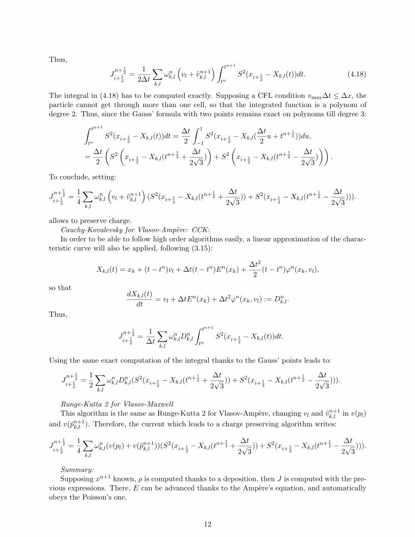
damping associated to k = 0.5, which is −0.1533 is added in order to ensure that the solutioncorresponds to the predicted damping. On the same figure is plotted the same result with a CFLcondition superior than 1 for RK2 and CRK2, which proves that the problem comes from theviolation of the CFL condition in the charge algorithm. In particular, we also plot on Fig. 2 andon Fig. 3 the charge conservation and the Ampere-Poisson equivalence with on the left CFL < 1,and on the right CFL > 1. These results are issued from the RK algorithm and are given after1000 iterations.

For the CK algorithm, we just plot on Fig. 4 on the left the electric energy and the theoreticaldamping for CK2 presented in section 3.2 and CCK2 presented in section 4, with CFL< 1, and thesame on the right for CK3 and CCK3 developed in the same sections. The curves are overlayed,as it was expected.

-22-20-18-16-14-12-10

-8-6-4

0 20 40 60 80 100

Ele

ctri

c en

erg

y

Time !p-1

Linear Landau damping

RK2CRK2

damping

-22-20-18-16-14-12-10

-8-6-4

0 20 40 60 80 100

Ele

ctri

c en

erg

y

Time !p-1


CRK2RK2

damping

Figure 1: Linear Landau damping for k = 0.5 Nx = Nv = 64, ∆t = 0.03 (left); ∆t = 0.1 (right).

-6e-15-5e-15-4e-15-3e-15-2e-15-1e-15

0 1e-15 2e-15 3e-15 4e-15 5e-15

0 2 4 6 8 10 12 14

Ch

arg

e co

nse

rvat

ion

x

Linear Landau Damping

CRK2

-6e-08-5e-08-4e-08-3e-08-2e-08-1e-08

0 1e-08 2e-08 3e-08

0 2 4 6 8 10 12 14

Ch

arg

e co

nse

rvat

ion

x


CRK2

Figure 2: Charge Conservation Nx = Nv = 64, ∆t = 0.03 (left); ∆t = 0.1 (right), 1000 iterations.

14

0

5e-13

1e-12

1.5e-12

2e-12

2.5e-12

0 2 4 6 8 10 12 14Eq

uiv

alen

ce A

mp

ere

Po

isso

n

x


CRK2

0 5e-07 1e-06

1.5e-06 2e-06

2.5e-06 3e-06

3.5e-06 4e-06

0 2 4 6 8 10 12 14Eq

uiv

alen

ce A

mp

ere

Po

isso

n

x


CRK2

Figure 3: Ampere-Poisson equivalence, Nx = Nv = 64, ∆t = 0.03 (left); ∆t = 0.1 (right), 1000iterations.

-22-20-18-16-14-12-10

-8-6-4

0 20 40 60 80 100

Ele

ctri

c en

erg

y

Time !p-1


CK2CCK2

damping

-22-20-18-16-14-12-10

-8-6-4

0 20 40 60 80 100

Ele

ctri

c en

erg

y

Time !p-1


CK3CCK3

damping

Figure 4: Electric energy for CK2 (left) and CK3 (right) Nx = Nv = 64, ∆t = 0.03.

5.3 Two stream instability

This test case simulates two beams with opposite velocities that encounter (see [17, 26]). Thecorresponding initial condition can be given by

f0(x, v) =M(v)v2[1− α cos(kx)], M(v) =1√2π

exp

(−v

2

2

),

with k = 0.5 and α = 0.05. The computational domain is [0, 2π/k] × [−9, 9] which is sampledby Nx = Nv = 128 points. For the charge conservation algorithms developed in section 4, CFLimposes ∆t < 0.0109, so the case CFL< 1 will be made with ∆t = 0.01, and CFL> 1 with∆t = 0.1. We are interested in the electric energy 1/2‖E(t)‖2L2 , which will be displayed in logscale. The same quantities as for the previous test cases are plotted on Fig. 5, 6, 7 and 8. The

15

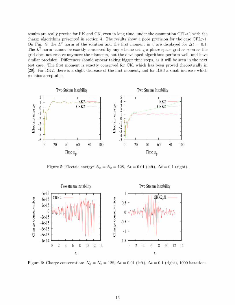
results are really precise for RK and CK, even in long time, under the assumption CFL<1 with thecharge algorithms presented in section 4. The results show a poor precision for the case CFL>1.On Fig. 9, the L2 norm of the solution and the first moment in v are displayed for ∆t = 0.1.The L2 norm cannot be exactly conserved by any scheme using a phase space grid as soon as thegrid does not resolve anymore the filaments, but the developed algorithms perform well, and havesimilar precision. Differences should appear taking bigger time steps, as it will be seen in the nexttest case. The first moment is exactly conserved for CK, which has been proved theoretically in[29]. For RK2, there is a slight decrease of the first moment, and for RK3 a small increase whichremains acceptable.

-6-5-4-3-2-1 0 1 2

0 20 40 60 80 100

Ele

ctri

c en

erg

y

Time !p-1

Two Stream Instability

RK2CRK2

-5-4-3-2-1 0 1 2 3 4 5

0 20 40 60 80 100

Ele

ctri

c en

erg

y

Time !p-1


RK2CRK2

Figure 5: Electric energy: Nx = Nv = 128, ∆t = 0.01 (left), ∆t = 0.1 (right).

-1e-14-8e-15-6e-15-4e-15-2e-15

0 2e-15 4e-15 6e-15

0 2 4 6 8 10 12 14

Ch

arg

e co

nse

rvat

ion

x

Two stream instability

CRK2

-1.5

-1

-0.5

0

0.5

1

0 2 4 6 8 10 12 14

Ch

arg

e co

nse

rvat

ion

x


CRK2cfl

Figure 6: Charge conservation: Nx = Nv = 128, ∆t = 0.01 (left), ∆t = 0.1 (right), 1000 iterations.

16

0 1e-12 2e-12 3e-12 4e-12 5e-12 6e-12 7e-12 8e-12

0 2 4 6 8 10 12 14Eq

uiv

alen

ce A

mp

ere

Po

isso

n

x


CRK2

0 20 40 60 80

100 120 140 160

0 2 4 6 8 10 12 14Eq

uiv

alen

ce A

mp

ere

Po

isso

n

x


CRK2

Figure 7: Ampere-Poisson equivalence, Nx = Nv = 128, ∆t = 0.01 (left), ∆t = 0.1 (right), 1000iterations.

-6-5-4-3-2-1 0 1 2

0 20 40 60 80 100

Ele

ctri

c en

erg

y

Time !p-1


CK2CCK2

-6-5-4-3-2-1 0 1 2

0 20 40 60 80 100

Ele

ctri

c en

erg

y

Time !p-1


CK3CCK3

Figure 8: Electric energy CK2 (left) CK3 (right) Nx = Nv = 128, ∆t = 0.01.

17

-0.03-0.025

-0.02-0.015

-0.01-0.005

0

0 20 40 60 80 100

L2 n

orm

Time !p-1


RK2RK3CK2CK3

-1e-07 0

1e-07 2e-07 3e-07 4e-07 5e-07 6e-07 7e-07 8e-07

0 20 40 60 80 100

1st

Mo

men

tum

Time !p-1


RK2RK3CK2CK3

Figure 9: L2 norm (left), First moment in v (right) ∆t = 0.1.

5.4 Bump on Tail

Next, we can apply the scheme to the bump-on-tail instability test case for which the initialcondition writes (see [32])

f0(x, v) = f(v)[1 + α cos(kx)],

with α = 0.04, k = 0.3 and

f(v) =np√2π

exp(−v2/2) +nb√2π

exp

(−|v − u|

2

2v2t

),

on the interval [0, 20π], with periodic conditions in space. The initial condition f0 is a Maxwelliandistribution function which has a bump on the Maxwell distribution tail; the physical parametersare the following

np = 0.9, nb = 0.2, u = 4.5, vt = 0.5,

whereas the numerical parameters are Nx = 128, Nv = 128, vmax = 9. For the charge conservationalgorithms, CFL imposes ∆t < 0.0545, so the cases CFL< 1 will be made with ∆t = 0.05, and CFL> 1 with ∆t = 0.2. We still give the same diagnostics on Fig. 10, 11, 12 and 13. For this electricenergy diagnostic, we expect oscillatory behavior of frequency equal to 1.05; moreover, since aninstability will be declared, the electric energy has to increase up to saturation at t ≈ 20.95 and toconverge for large times (see [26, 32]). The results are really precise for RK and CK, even in longtime, under the assumption CFL< 1 for the charge algorithms developed in section 4.

On Fig. 14, the L2 norm of the distribution function and the entropy −∫f ln(f) dxdv are

plotted for ∆t = 0.2. These two quantities are known to be theoretically preserved. As it wasalready explained, this cannot be reached with our kind of numerical methods. The conservationproperties are better for the third order CK3 and RK3 than for the second order CK2 and RK2.Let us precise that more ∆t increases, more these differences are important, and that the RKalgorithms perform a bit better, but are more expensive computationaly speaking.

18

0 1 2 3 4 5 6 7 8 9

0 50 100 150 200 250 300 350 400

Ele

ctri

c en

erg

y

Time !p-1

Bump on Tail

RK2CRK2

0 1 2 3 4 5 6 7 8 9

0 50 100 150 200 250 300 350 400

Ele

ctri

c en

erg

y

Time !p-1

Bump on Tail

RK2CRK2

Figure 10: Electric energy ∆t = 0.05 (left) ∆t = 0.2 (right).

-8e-15-6e-15-4e-15-2e-15

0 2e-15 4e-15 6e-15

0 10 20 30 40 50 60 70

Ch

arg

e co

nse

rvat

ion

x

Bump on Tail

CRK2

-0.008-0.006-0.004-0.002

0 0.002 0.004 0.006 0.008

0.01

0 10 20 30 40 50 60 70

Ch

arg

e co

nse

rvat

ion

x

Bump on Tail

CRK2

Figure 11: Charge Conservation ∆t = 0.05 (left) ∆t = 0.2 (right).

19

0 5e-13 1e-12

1.5e-12 2e-12

2.5e-12 3e-12

3.5e-12 4e-12

4.5e-12

0 10 20 30 40 50 60 70Eq

uiv

alen

ce A

mp

ere

Po

isso

n

x

Bump on Tail

CRK2

0 0.001 0.002 0.003 0.004 0.005 0.006 0.007 0.008 0.009

0.01

0 10 20 30 40 50 60 70Eq

uiv

alen

ce A

mp

ere

Po

isso

n

x

Bump on Tail

CRK2

Figure 12: Ampere-Poisson equivalence ∆t = 0.05 (left) ∆t = 0.2 (right).

0 1 2 3 4 5 6 7 8 9

0 50 100 150 200 250 300 350 400

Ele

ctri

c en

erg

y

Time !p-1

Bump on Tail

CK2CCK2

0 1 2 3 4 5 6 7 8 9

0 50 100 150 200 250 300 350 400

Ele

ctri

c en

erg

y

Time !p-1

Bump on Tail

CK3CCK3

Figure 13: Electric energy ∆t = 0.05, CK2 (left), CK3 (right).

20

-0.012-0.01

-0.008-0.006-0.004-0.002

0

0 50 100 150 200 250 300 350 400

L2 n

orm

Time !p-1

Bump on Tail

RK2RK3CK2CK3

13.35 13.4

13.45 13.5

13.55 13.6

13.65 13.7

0 50 100 150 200 250 300 350 400

En

tro

py

Time !p-1

Bump on Tail

RK2RK3CK2CK3

Figure 14: L2 norm (left), Entropy (right) ∆t = 0.2.

5.5 QR Vlasov-Maxwell test case

The numerical method used to solve this test case was presented in section 2.2. Let us precise thenumerical parameters used to perform this test case.

f0(x, p) =1√2πT

exp

(− p2

(2T 2)

)(1 + cos(kx)),

T = 3keV , and k = 1√2. A circularly polarized electromagnetic wave is initialized in a periodic

domain with a quiver momentum a0 =√

3:

E0y(x) = E0 cos(kx) E0

z (x) = E0 sin(kx)

B0y(x) =

−k∗E0

ω0sin(kx) B0

z (x) =k∗E0

ω0cos(kx)

A0y(x) = −E0

ω0sin(kx) A0

z(x) =E0

ω0cos(kx)

where k∗ = k sinc(k∆x2 ), and sinc(x) = sin(x)

x . We consider a pump wave of frequency ω0 and

wavenumber k0 such that ω20 = ω2

p/γ0 +k20c

2 is satisfied, with γ0 = 1+a20. Choosing k0c/m = 1/

√2,

we obtain ω0/ωp = 1 (i.e. a ratio n/nc = 1). ωp is the plasma frequency, c the light velocity andnc the critical density.

These physical parameters correspond to the most unstable mode, for more details about thetest case, see [21, 22]. The numerical parameters are chosen as follows: the impulsion domain is[−pmax, pmax], where pmax = 8.5. The choice of k0 determines the size of the periodic space domainwhich is taken equal to [0, 2π

√2], Nx = 256, Np = 256, ∆t = 0.01, which is under CFL condition.

We display on Fig. 15, 16, 17, 18, the distribution function at different times, for a Backwardsemi-Lagrangian algorithm, which shall be our reference, and our FSL charge conserving algorithmintroduced in section 4. The two methods are difficult to compare with only this diagnostic, andseem to behave similarly. On Fig. 19, the mass conservation for BSL and FSL is plotted. FSLbehaves far better, especially with long time scaling. Obviously, as the mass decreases, the chargecannot be conserved anymore, which is shown on Fig. 20, 21. Before the decrease of the mass, the

21

FSL algorithm preserves charge exactly, and after the decrease, remains truly better. To conclude,on Fig. 22, 23 the integration of f with respect to x is displayed, at different times. At thebeginning, the two curves are very close, but as time goes on, the two curves separate, and FSLremains more centered than BSL. For more details about comparisons between FSL and BSL, thereader is refered to [10].

Figure 15: Distribution function at time = 10 and 22, Nx = 256, Np = 256,∆t = 0.01.

Figure 16: Distribution function at time = 23, BSL vs FSL, Nx = 256, Np = 256,∆t = 0.01.

22



23

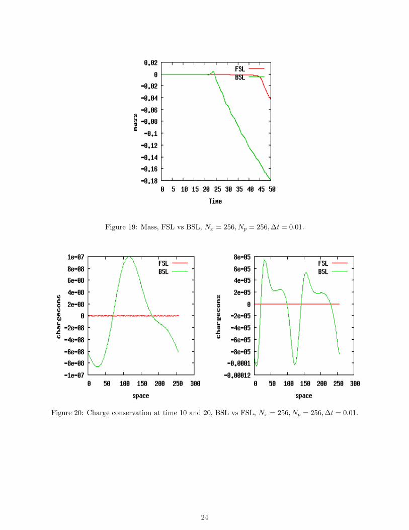
Figure 19: Mass, FSL vs BSL, Nx = 256, Np = 256,∆t = 0.01.

Figure 20: Charge conservation at time 10 and 20, BSL vs FSL, Nx = 256, Np = 256,∆t = 0.01.

24

Figure 21: Charge conservation at time 26 and 30, BSL vs FSL, Nx = 256, Np = 256,∆t = 0.01.

Figure 22: Integration of f along x, t = 1000 and 2000, BSL vs FSL,Nx = 256, Np = 256,∆t = 0.01.

25

Figure 23: Integration of f along x, t = 30 and 40, BSL vs FSL Nx = 256, Np = 256,∆t = 0.01.

5.6 Numerical Synthesis

One of our goals was to compare these different algorithms in order to choose the best one for aprospective work in view of tackling the 4D case. First, it has to be said that the CK procedure isfaster than the RK one, especially when you look for high order simulation, merely because thereare no intermediate deposition steps, which is one of the most expensive step. Obviously, in CCKmethods, a 2D deposition is made to compute J , therefore the CPU time is the same as the oneof RK (see Table 1). The results concerning electric energy are really difficult to compare, andseem very good whatever algorithm you choose. We observe that the conserved quantities, likethe L2 norm of the distribution function are a bit better with RK, so CRK seems to be a goodcompromise between cost and accuracy. These methods are validated by these 1D test cases, andare encouraging for prospective work.

RK2 RK3 Verlet CK2 CK3 CRK2 CCK2 CCK3

64× 64 27.1 s. 42.5 s. 26 s. 19 s. 20.8 s. 27.6 s. 27.1 s. 42.5 s.

Table 1: Comparison of the CPU time of the different methods. 10000 iterations.

Moreover, with the last test case, with real Maxwell’s equations, we see that a charge conservingFSL method is really better than a classical BSL one, which is entirely satisfying, and convincingfor future work.

6 Conclusion

In this paper, charge preserving Forward semi-Lagrangian algorithms of second and third order forthe characteristics have been developed, and the numerical results meet requirements for varioustest cases. In these cases, under a CFL condition, the two methods Vlasov-Poisson and Vlasov-Ampere have proven to be exactly the same, and the charge has proved to be preserved. A future

26

work will be to design a 4D charge preserving FSL Vlasov-Maxwell scheme, especially comparingcharge preserving algorithms developed in [30] with a procedure derived from this work, using asplitting scheme.

References

[1] R. Barthelme, Le probleme de conservation de la charge dans le couplage des equations deVlasov et de Maxwell, These de l’Universite Louis Pasteur, 2005.

[2] M. Bostan, N. Crouseilles, Convergence of a semi-Lagrangian scheme for the reducedVlasov-Maxwell sytem for laser-plasma interaction, Numer. Math. 112, no2, pp. 169-195 (2009).

[3] C.K. Birdsall, A.B. Langdon, Plasma Physics via Computer Simulation, Inst. of Phys.Publishing, Bristol/Philadelphia, (1991).

[4] F. Bouchut, F. Golse, M. Pulvirenti, Kinetic equations and asymptotic theory, Series inapplied Math. P.G Ciarlet and P.L Lions (Eds) Gauthier Villars (2008).

[5] J. A. Carrillo, S. Labrunie, Global solutions for the one-dimensional Vlasov-Maxwell sys-tem for laser-plasma interaction, Math. Models Methods Appl. Sci. 16, pp. 19-57, (2006).

[6] J.-A. Carrillo, F. Vecil, Non oscillatory interpolation methods applied to Vlasov-basedmodels, SIAM Journal of Sc. Comput. 29, pp. 1179-1206, (2007).

[7] C. Z. Cheng, G. Knorr, The integration of the Vlasov equation in configuration space, J.Comput. Phys, 22, pp. 330-3351, (1976).

[8] P. Colella, P.R. Woodward, The Piecewise Parabolic Method (PPM) for gas-dynamicalsimulations, J. Comput. Phys. 54 (1984) 174–201.

[9] N. Crouseilles, M. Mehrenberger, E. Sonnendrucker, Conservative semi-Lagrangianschemes for the Vlasov equation, J. Comput. Phys., 229, no6, pp. 1927-1953 (2010).

[10] N. Crouseilles, T. Respaud, E. Sonnendrucker, A forward semi-Lagrangian methodfor the numerical solution of the Vlasov equation, Comput. Phys. Comm. 180, pp.1730-1745,(2009).

[11] N. Crouseilles, A. Ghizzo, S. Salmon, Vlasov laser-plasma interaction simulations witha moving grid, INRIA Research Report number 6109 (2007).

[12] C.J. Cotter, J. Frank, S. Reich The remapped particle-mesh semi-Lagrangian advectionscheme, Q. J. Meteorol. Soc., 133, pp. 251-260, (2007).

[13] J.W. Eastwood, Virtual particle methods, Comp. Phys. Comm., 64, Issue 2, pp. 252-266,(1991).

[14] N.V. Elkina, J. Buchner, A new conservative unsplit method for the solution of the Vlasovequation, J. Comput. Phys. 213 pp. 862, (2006).

[15] T. Zh. Esirkepov, Exact charge conservation scheme for Particle-in-Cell simulation with anarbitrary form-factor, Comp. Phys. Comm. 135, pp. 144-153, (2001).

[16] F. Filbet, E. Sonnendrucker, P. Bertrand, Conservative numerical schemes for theVlasov equation, J. Comput. Phys., 172, pp. 166-187, (2001).

27

[17] F. Filbet, E. Sonnendrucker, Comparison of Eulerian Vlasov solvers, Comput. Phys.Comm., 151, pp. 247-266, (2003).

[18] A. Ghizzo, P. Bertrand, M.L. Begue, T.W. Johnston, M. Shoucri, A Hilbert-Vlasovcode for the study of high-frequency plasma beatwave accelerator, IEEE Transaction on PlasmaScience, 24, p. 370, (1996).

[19] A. Ghizzo, P. Bertrand, M. Shoucri, T.W. Johnston, E. Fijalkow, M.R. Feix, AVlasov code for the numerical simulation of stimulated Raman scattering, J. Comput. Phys. 90,pp. 431-457, (1990).

[20] V. Grandgirard, M. Brunetti, P. Bertrand, N. Besse, X. Garbet, P. Ghendrih,G. Manfredi, Y. Sarrazin, O. Sauter, E. Sonnendrucker, J. Vaclavik, L. Villard,A drift-kinetic semi-Lagrangian 4D code for ion turbulence simulation, J. Comput. Phys., 217,pp. 395-423, (2006).

[21] F. Huot, A. Ghizzo, P. Bertrand, E. Sonnendrucker, O. Coulaud Instability ofthe time splitting scheme for the one-dimensional and relativistic Vlasov-Maxwell system, J.Comput. Phys., 185, pp. 512-531, (2003).

[22] F. Huot, A. Ghizzo, P. Bertrand, E. Sonnendrucker, O. Coulaud Study of a propa-gation of ultraintense electromagnetic wave through plasma using semi-Lagrangian Vlasov codes,IEEE Trans. on Plasma SC., 28, (2000).

[23] T.W. Johnston, P. Bertrand, A. Ghizzo, M. Shoucri, E. Fijalkow, M.R. Feix,Simulated Raman scattering: Action evolution and particle trapping via Euler-Vlasov, fluidsimulation, Phys. Fluids B4, pp. 2523-2537, (1992).

[24] B. Marder, A method for incorporating Gauss’s law into electromagnetic PIC codes, J. Com-put. Phys. 68, pp. 48-55, (1987).

[25] C.-D. Munz, P. Omnes, R. Schneider, E. Sonnendrucker, U. Voss, Divergence Cor-rection Techniques for Maxwell Solvers Based on a Hyperbolic Model, J. Comput. Phys., 161,Issue 2, pp. 484-511, (2000).

[26] T. Nakamura, T. Yabe, Cubic interpolated propagation scheme for solving the hyper-dimensional Vlasov-Poisson equation in phase space, Comput. Phys. Comm., 120, pp. 122-154,(1999).

[27] E. Pohn, M. Shoucri, M. Kamelander, Comp. Phys. Comm. 137 , pp. 380-395 (2001).

[28] S. Reich, An explicit and conservative remapping strategy for semi-Lagrangian advection,Atmospheric Science Letters, 8, pp. 58-63, (2007).

[29] T. Respaud, E. Sonnendrucker Analysis of a new class of Forward semi-Lagrangianschemes for the 1D Vlasov Poisson Equations, HAL: hal-00442957, Submitted.

[30] N.J. Sircombe, T.D. Arber, VALIS: A split-conservative scheme for the relativistic 2D ; J.Comput. Phys., 228, pp. 4773-4788 (2009).

[31] M. Shoucri, A two-level implicit scheme for the numerical solution of the linearized vorticityequation, Int. J. Numer. Meth. Eng., 17, p. 1525 (1981).

[32] M. Shoucri, Nonlinear evolution of the bump-on-tail instability, Phys. Fluids, 22, p. 2038-2039 (1979).

28

[33] H. Schmitz, R. Grauer, Comparison of time splitting and backsubstitution methods forintegrating Vlasov’s equation with magnetic fields, Comput. Phys. Commun. 175, pp.86 (2006).

[34] E. Sonnendrucker, J. Roche, P. Bertrand, A. Ghizzo, The semi-Lagrangian methodfor the numerical resolution of the Vlasov equation, J. Comput. Phys., 149, pp. 201-220, (1999).

[35] T. Umeda, Y. Omura, T. Tominaga, H. Matsumoto, A new charge conservation methodin electromagnetic particle-in-cell simulations, Comp. Phys. Comm 156, Issue1, pp. 73-85,(2003).

[36] J. Villasenor, O. Buneman, Rigorous charge conservation for local electromagnetic fieldsolvers, Comp. Phys. Comm. 69, pp. 306-316, (1992).

[37] M. Zerroukat, N. Wood, A. Staniforth, A monotonic and positive-definite filter for aSemi-Lagrangian Inherently Conserving and Efficient (SLICE) scheme, Q.J.R. Meteorol. Soc.,131, pp 2923-2936, (2005).

[38] M. Zerroukat, N. Wood, A. Staniforth, The Parabolic Spline Method (PSM) for con-servative transport problems, Int. J. Numer. Meth. Fluids, 51, pp. 1297-1318, (2006).

29

Documents

A charge preserving scheme for the numerical resolution of