IOP PUBLISHING JOURNAL OF PHYSICS B: ATOMIC, MOLECULAR AND OPTICAL PHYSICS

J. Phys. B: At. Mol. Opt. Phys. 46 (2013) 235003 (10pp) doi:10.1088/0953-4075/46/23/235003

A classical analogue for adiabatic Starksplitting in non-hydrogenic atomsG W Gordon and F Robicheaux1

Department of Physics, Auburn University, AL 36849, USA

E-mail: robichf@purdue.edu

Received 15 July 2013, in final form 10 October 2013Published 11 November 2013Online at stacks.iop.org/JPhysB/46/235003

AbstractFor highly excited low-� states of atoms, a rising electric field causes a mixing betweenangular momenta that gives rise to Stark states. A relatively simple situation occurs if theelectric field is not strong enough to mix states with adjacent principle quantum numbers. Ifthe initial state has slightly lower (higher) energy than the degenerate manifold, then the stateadiabatically connects to a Stark state with the electron on the low (high) potential energy sideof the atom. We show that purely classical calculations for non-hydrogenic atoms have anadiabatic connection to extreme dipole moments similar to quantum systems. We use a simplemap to show that the classical dynamics arises from the direction of the precession of theRunge–Lenz vector when the electric field is off. As a demonstration of the importance of thiseffect, we perform classical calculations of charge exchange and show that the total crosssection for charge transfer and for ionization strongly depend on whether or not a pureCoulomb potential is used.

1. Introduction

The behaviour of a highly excited atom in an electric fieldhas been studied since the dawn of quantum mechanics.Besides the experimental studies, there have been classical,semiclassical, and quantum treatments of this system. Wegive a brief survey of recent results. For example, [1, 2]describe fully classical treatments of H in weak electric fields.Reference [3] measured the Rb spectrum in a strong electricfield and showed that there were resonance states above theclassical threshold as well as above the zero-field threshold; afully quantum treatment [4] gave quantitative agreement withthis type of measurement. The non-hydrogenic part of thepotential leads to strong changes from a purely hydrogeniccase. A series of experiments and semiclassical and quantumcalculations elucidated the importance of elastic scatteringfrom the non-Coulombic part of the potential for the Starkspectra of atoms (some examples are [5–9]). In addition totime independent studies, there were several investigationsbased on time dependent motion of the electron probability(some examples are [10–14]). There are fewer purely classicalstudies of the non-hydrogenic Stark case; [15] investigated

1 Present address: Department of Physics, Purdue University, West Lafayette,IA 47907, USA.

how a small polarizability of the core affected the motionand [16] performed a classical calculation of how a non-hydrogenic atom is ionized in a low frequency microwave field.In many of the theoretical studies, a fully quantum treatmentwas compared to a semiclassical treatment; [17] investigatedhow the linear and the quadratic Stark shift in H comparedbetween a quantum and a fully classical treatment.

In this study, we investigate how a classical non-hydrogenic atom responds to a slowly ramped electric field. Anextreme example of this is state selective field ionization [18]in which the electron is eventually pulled from the atom; stateselective field ionization is difficult to treat fully quantummechanically [19] because of the long time scales involved.For electric fields that are not strong enough to mix statesof different principle quantum number, an electric field giveseigenstates with an electric dipole moment that can have theelectron on the high (low) potential energy side of the atom.These are states whose energy shifts up (down) with increasingelectric field strength. If the electric field is in the +z-direction,the high potential energy side of the atom for the electron haspositive z.

The non-relativistic hydrogen atom is particularly simplein that the eigenstates only weakly depend on the electricfield strength until the n-mixing regime. The situation isslightly more complicated for non-hydrogenic atoms [18].

0953-4075/13/235003+10$33.00 1 © 2013 IOP Publishing Ltd Printed in the UK & the USA

J. Phys. B: At. Mol. Opt. Phys. 46 (2013) 235003 G W Gordon and F Robicheau

(a) (b)

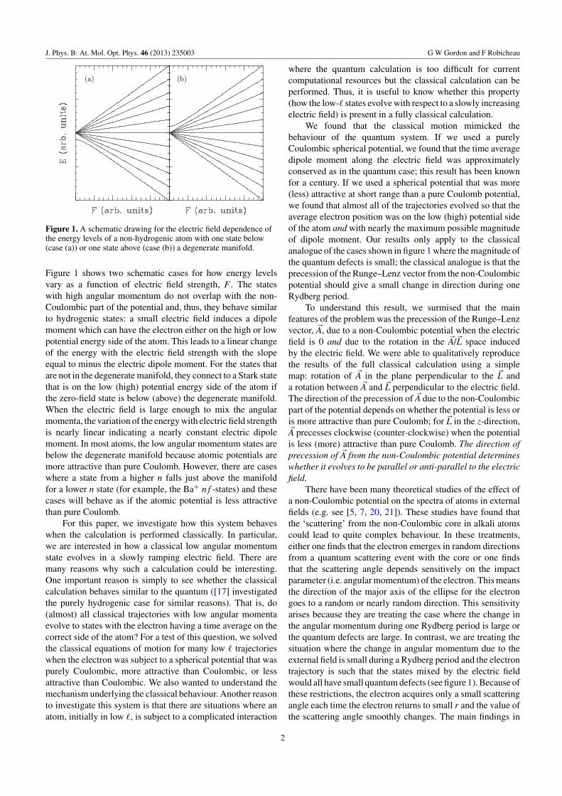
Figure 1. A schematic drawing for the electric field dependence ofthe energy levels of a non-hydrogenic atom with one state below(case (a)) or one state above (case (b)) a degenerate manifold.

Figure 1 shows two schematic cases for how energy levelsvary as a function of electric field strength, F . The stateswith high angular momentum do not overlap with the non-Coulombic part of the potential and, thus, they behave similarto hydrogenic states: a small electric field induces a dipolemoment which can have the electron either on the high or lowpotential energy side of the atom. This leads to a linear changeof the energy with the electric field strength with the slopeequal to minus the electric dipole moment. For the states thatare not in the degenerate manifold, they connect to a Stark statethat is on the low (high) potential energy side of the atom ifthe zero-field state is below (above) the degenerate manifold.When the electric field is large enough to mix the angularmomenta, the variation of the energy with electric field strengthis nearly linear indicating a nearly constant electric dipolemoment. In most atoms, the low angular momentum states arebelow the degenerate manifold because atomic potentials aremore attractive than pure Coulomb. However, there are caseswhere a state from a higher n falls just above the manifoldfor a lower n state (for example, the Ba+ n f -states) and thesecases will behave as if the atomic potential is less attractivethan pure Coulomb.

For this paper, we investigate how this system behaveswhen the calculation is performed classically. In particular,we are interested in how a classical low angular momentumstate evolves in a slowly ramping electric field. There aremany reasons why such a calculation could be interesting.One important reason is simply to see whether the classicalcalculation behaves similar to the quantum ([17] investigatedthe purely hydrogenic case for similar reasons). That is, do(almost) all classical trajectories with low angular momentaevolve to states with the electron having a time average on thecorrect side of the atom? For a test of this question, we solvedthe classical equations of motion for many low � trajectorieswhen the electron was subject to a spherical potential that waspurely Coulombic, more attractive than Coulombic, or lessattractive than Coulombic. We also wanted to understand themechanism underlying the classical behaviour. Another reasonto investigate this system is that there are situations where anatom, initially in low �, is subject to a complicated interaction

where the quantum calculation is too difficult for currentcomputational resources but the classical calculation can beperformed. Thus, it is useful to know whether this property(how the low-� states evolve with respect to a slowly increasingelectric field) is present in a fully classical calculation.

We found that the classical motion mimicked thebehaviour of the quantum system. If we used a purelyCoulombic spherical potential, we found that the time averagedipole moment along the electric field was approximatelyconserved as in the quantum case; this result has been knownfor a century. If we used a spherical potential that was more(less) attractive at short range than a pure Coulomb potential,we found that almost all of the trajectories evolved so that theaverage electron position was on the low (high) potential sideof the atom and with nearly the maximum possible magnitudeof dipole moment. Our results only apply to the classicalanalogue of the cases shown in figure 1 where the magnitude ofthe quantum defects is small; the classical analogue is that theprecession of the Runge–Lenz vector from the non-Coulombicpotential should give a small change in direction during oneRydberg period.

To understand this result, we surmised that the mainfeatures of the problem was the precession of the Runge–Lenzvector, �A, due to a non-Coulombic potential when the electricfield is 0 and due to the rotation in the �A/�L space inducedby the electric field. We were able to qualitatively reproducethe results of the full classical calculation using a simplemap: rotation of �A in the plane perpendicular to the �L anda rotation between �A and �L perpendicular to the electric field.The direction of the precession of �A due to the non-Coulombicpart of the potential depends on whether the potential is less oris more attractive than pure Coulomb; for �L in the z-direction,�A precesses clockwise (counter-clockwise) when the potentialis less (more) attractive than pure Coulomb. The direction ofprecession of �A from the non-Coulombic potential determineswhether it evolves to be parallel or anti-parallel to the electricfield.

There have been many theoretical studies of the effect ofa non-Coulombic potential on the spectra of atoms in externalfields (e.g. see [5, 7, 20, 21]). These studies have found thatthe ‘scattering’ from the non-Coulombic core in alkali atomscould lead to quite complex behaviour. In these treatments,either one finds that the electron emerges in random directionsfrom a quantum scattering event with the core or one findsthat the scattering angle depends sensitively on the impactparameter (i.e. angular momentum) of the electron. This meansthe direction of the major axis of the ellipse for the electrongoes to a random or nearly random direction. This sensitivityarises because they are treating the case where the change inthe angular momentum during one Rydberg period is large orthe quantum defects are large. In contrast, we are treating thesituation where the change in angular momentum due to theexternal field is small during a Rydberg period and the electrontrajectory is such that the states mixed by the electric fieldwould all have small quantum defects (see figure 1). Because ofthese restrictions, the electron acquires only a small scatteringangle each time the electron returns to small r and the value ofthe scattering angle smoothly changes. The main findings in

2

J. Phys. B: At. Mol. Opt. Phys. 46 (2013) 235003 G W Gordon and F Robicheau

this paper would need to be revisited if the electron starts withsmall angular momentum so that the scattering angle is largeand sensitively dependent on the precise value of the impactparameter or the field is so large that the change in angularmomentum during one Rydberg period is sufficient to take theelectron from large angular momentum (where the scatteringangle is small and not sensitive) to small angular momentum(where the scattering angle is large and sensitive).

To show that this result can be important in practice, weperformed classical calculations of ion–atom scattering. Aswith studies of the simple Stark effect, ion–atom scattering forhighly excited states has a long history. For example, [22–24]experimentally studied �-changing and n-changing collisionsas well as charge transfer. Several theoretical studies [25–29]have investigated most aspects of this system. In the lastsection, we investigate charge transfer and ionization in ion–atom scattering where the target atom is initially in a lowangular momentum state. The early stages of the scatteringinvolve weak and slowly varying electric fields which caninduce the electron to adiabatically connect to either red orblue Stark states depending on the initial quantum defect. Wefound that even the total cross sections depended on whetherthe target atom had a pure Coulomb potential or whether thepotential was more or was less attractive than pure Coulomb.This effect does not appear to have been noticed previously.

2. Classical model

The classical equations of motion can be solved with a varietyof techniques. We used an adaptive step-size Runge–Kuttamethod based on the one described in [30]. With this method,we solve the six coupled, first-order differential equations.As a consistency check in the calculations, we make surethat any conserved quantity changes by less than a part in105. As an additional check and for the cases where therewere no conserved quantities, we compared distributions ofphysical parameters at the end of runs using different levels ofconvergence.

We chose a simple form for the non-Coulombic potentialwhich allowed us to smoothly vary from more attractive, topure Coulomb, to less attractive. The form we chose for thepotential energy was

V (r) = − e2

4πε0

1 + C exp(−r/a0)

r(1)

where a0 is the Bohr radius and C is an adjustable constant.When C > 0 (C < 0), the potential is more (less) attractivethan pure Coulomb. Of course, the case of C = 0 is hydrogen.We only show results below for the cases C = 1, 0, and −1although we did check that other values gave similar results.

The motion of an electron in a non-Coulombic potentialand an electric field is complicated, but we found the Runge–Lenz vector facilitated an understanding of the motion. In ourdiscussions below, we use the scaled Runge–Lenz vector

�A =(

�p × �L − me2

4πε0r

)/√−2mE (2)

where �p is the electron’s momentum, m is the electron massand E is the energy of the electron. With this definition, the

�A points in the direction of the perihelion and has units ofangular momentum. For a pure Coulomb potential, the Runge–Lenz vector is a constant of the motion. Two non-Coulombicinteractions are important for understanding our results.

For a weak electric field in the z-direction, the angularmomentum and the Runge–Lenz vectors rotate into eachother:

d�L

dt= − ωz × �A

d�A

dt= − ωz × �L (3)

where ω = 3ea0nF/(2�) with n the principle quantum numberand F the electric field strength. From these equations, one canshow that Lz and Az are constants in a weak electric field. Theelectric field gives a rotation in Ax and Ly:

Ly(t) = Ly(0) cos(ωt) − Ax(0) sin(ωt)

Ax(t) = Ly(0) sin(ωt) + Ax(0) cos(ωt) (4)

with similar rotation for Ay and Lx.The other non-Coulombic interaction is from the spherical

potential for the electron for non-hydrogenic atoms. Thespherical potential does not change the angular momentumwith time. However, it does give a rotation of the Runge–Lenz vector in a plane perpendicular to the angular momentumduring each radial period. If the angular momentum is in they-direction, the equation of motion dβ/dt = Ly/(mr2) can beused to show that over a radial period the change in angle ofthe Runge–Lenz vector is

�β = 2∫ rmax

rmin

Ly

r2 p(r)dr − 2π (5)

where we used dt = dr/[p(r)/m], rmin is the innerturning point, rmax is the outer turning point, and p(r) =√

2m[E − Veff(r)] is the radial momentum with Veff =Vatom(r) + L2

y/(2mr2). Using this notation, after each radialperiod the Runge–Lenz vector rotates as

Az(TRyd) = Az(0) cos(�β) − Ax(0) sin(�β)

Ax(TRyd) = Az(0) sin(�β) + Ax(0) cos(�β) (6)

where TRyd is the Rydberg period. For the general case, |�L|replaces the Ly in equation (5) and the sense of rotation followsthe right hand rule in the plane perpendicular to �L.

Figure 2 shows how �β depends on angular momentumfor the potentials with C = 1 (solid line) and C = −1 (dottedline). For the potential more attractive than pure Coulomb(C = 1), there is a maximum in the precession angle at�y = Ly/� ∼ 1.5. The caseC = −1 is special in that it does nothave a singularity at r = 0 (although there is a discontinuity inthe derivative); this allows the electron to go straight throughthe origin for Ly = 0 which is why �β → −π as Ly → 0.

A last important feature is that the classical solution givesthe same answer for the same starting condition. Therefore, weneeded to make sure our results did not depend on the specificchoice of our initial condition. For a given starting position andvelocity, we averaged over the phase of the electron orbit by

3

J. Phys. B: At. Mol. Opt. Phys. 46 (2013) 235003 G W Gordon and F Robicheau

Figure 2. The change in angle per Rydberg period as a function of�y ≡ Ly/� for the case C = 1 (solid line) and the case C = −1(dotted line). Note there are three ways to connect the region ofnegative angular momentum to positive angular momentum: (a)�β(−�y) = −�β(�y), (b) �β(−�y) = 2π − �β(�y), or (c)�β(−�y) = −2π − �β(�y). Only one case gives continuitythrough the point � = 0. For the C = 1 potential, method (a) givescontinuity. For the C = −1 potential, method (c) gives continuity(also shown is method (a)).

running the field free case for a random fraction of a Rydbergperiod. We also made sure that the initial orientation of theorbit was not important. For a specified angular momentum �,we started the position at a random spot on the sphere definedby the aphelion with a flat distribution in cos(θ ) and in φ.To ensure a random orientation of the plane of motion withthe electric field set to 0, the velocity vector is chosen froma random distribution �v = (θ cos α + φ sin α)v where α ischosen from a random distribution.

3. Ramped electric field results: full classical

In this section, we present the results of our calculations wherewe slowly ramped on an electric field to a constant value. Aworry is that the electric field should smoothly turn on toavoid artefacts from discontinuities in the time derivative ofthe Hamiltonian. To avoid this we chose the time dependentelectric field to have a similar form from [31]:

F(t) = twid

tflatFmax ln

(1 + et/twid

1 + e(t−tflat )/twid

)(7)

where twid gives the effective time width over which thefield ramps on, tflat is approximately the time where the fieldbecomes constant and where Fmax is the maximum electricfield. This functional form has the property that it smoothlyincreases from 0 as t approaches 0 from below and thensmoothly becomes a linear function of time when t is largerthan twid. It then smoothly changes to a constant near the timet ∼ tflat.

In the calculations of this section, we chose twid =500TRydberg (i.e. 500 Rydberg periods) and tflat = twid. Ourresults were not sensitive to these values as long as theRunge–Lenz vector can precess many times during the ramp.This condition is the same as in the quantum atom. If theelectric field is turned on too rapidly, the states do not evolveadiabatically. In all of the cases, the maximum electric fieldstrength was 250 V m−1 (i.e. 2.5 V cm−1).

(a)

(b)

(c)

(d)

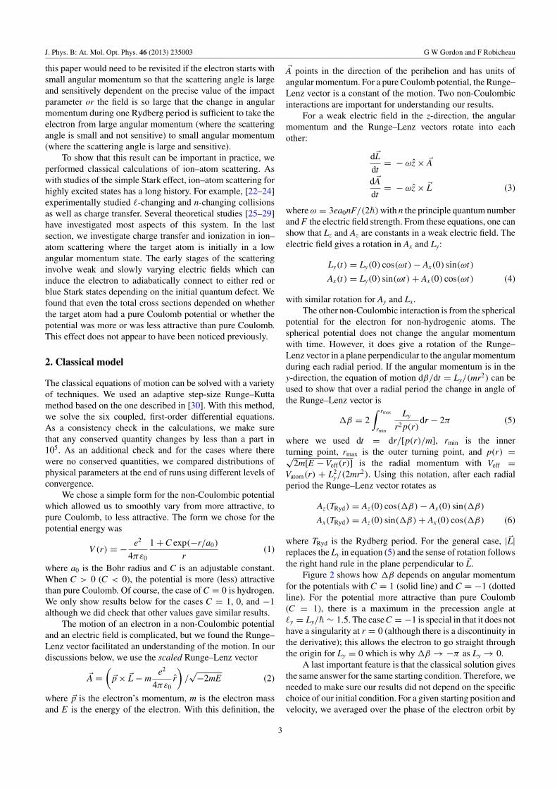
Figure 3. Trajectories in the zx-plane scaled by the atom sizern = 2n2a0. For all cases, Ly > 0 which means the angularmomentum is out of the page. (a) Trajectories for ∼10 Rydbergperiods when the electric field is 0: the case C = 0 (solid line) is asingle ellipse nearly vertical, the case C = 1 (dotted line) gives anellipse precessing counter-clockwise, and the case C = −1 (dashedline) gives an ellipse precessing clockwise. (b) Trajectories for∼200 Rydberg periods showing the precession due to an electricfield in the z-direction for C = 0. The z-component of theRunge–Lenze vector is conserved. The points of the trajectory are sodense it shows up as a black wedge instead of separate lines. (c)Same as (b) but for C = 1. The Runge–Lenz vector is no longerconstant. There are ∼8 Rydberg periods over which the direction ofthe major axis rotates counter-clockwise from ∼ − 25◦ to ∼25◦

relative to the −z-axis. (d) Same as (c) but for C = 1. Now thedirection of the major axis rotates clockwise from ∼ − 30◦ to ∼30◦

relative to the z-axis during ∼7 Rydberg periods.

To become oriented with how the classical electronbehaves, figure 3 shows six example trajectories: figure 3(a)shows trajectories with the electric field off for C = 0, −1, and1 while 3(b)–(d) show trajectories with an electric field in thez-direction. For all plots, the angular momentum is initially outof the page; only for figure 3(b) is the angular momentum intothe page for part of the trajectory. The case with no electricfield, figure 3(a), shows the precession due to a non-Coulombicforce compared to the trajectory for pure Coulomb which is anellipse slightly left of vertical; the C = 1 case gives counter-clockwise precession because the potential is deeper than pureCoulomb while the C = −1 case gives clockwise precession.Figure 3(b) shows the trajectory for pure Coulomb plus electric

4

J. Phys. B: At. Mol. Opt. Phys. 46 (2013) 235003 G W Gordon and F Robicheau

field in the z-direction. The trajectory has too many lines tosee the individual ellipses; qualitatively the major axis of theellipse oscillates within the black wedge with the minimumangular momentum at the edge of the wedge. Figure 3(c) showsthe C = 1 case with an electric field in the z-direction; thisis a late time part of the trajectory that arose from slowlyramping on the electric field. Note that the electron is on thelow potential energy side of the atom for most of the trajectory.There is a very rapid swing of the major axis around the atomin the counter-clockwise direction over a short period of time,∼8 Rydberg periods. Figure 3(d) shows the C = −1 casethat arose from slowly ramping on the electric field. Now theelectron is on the high potential energy side of the atom formost of the trajectory. Again, there is a rapid swing of the majoraxis around the atom, but now in the clockwise direction.

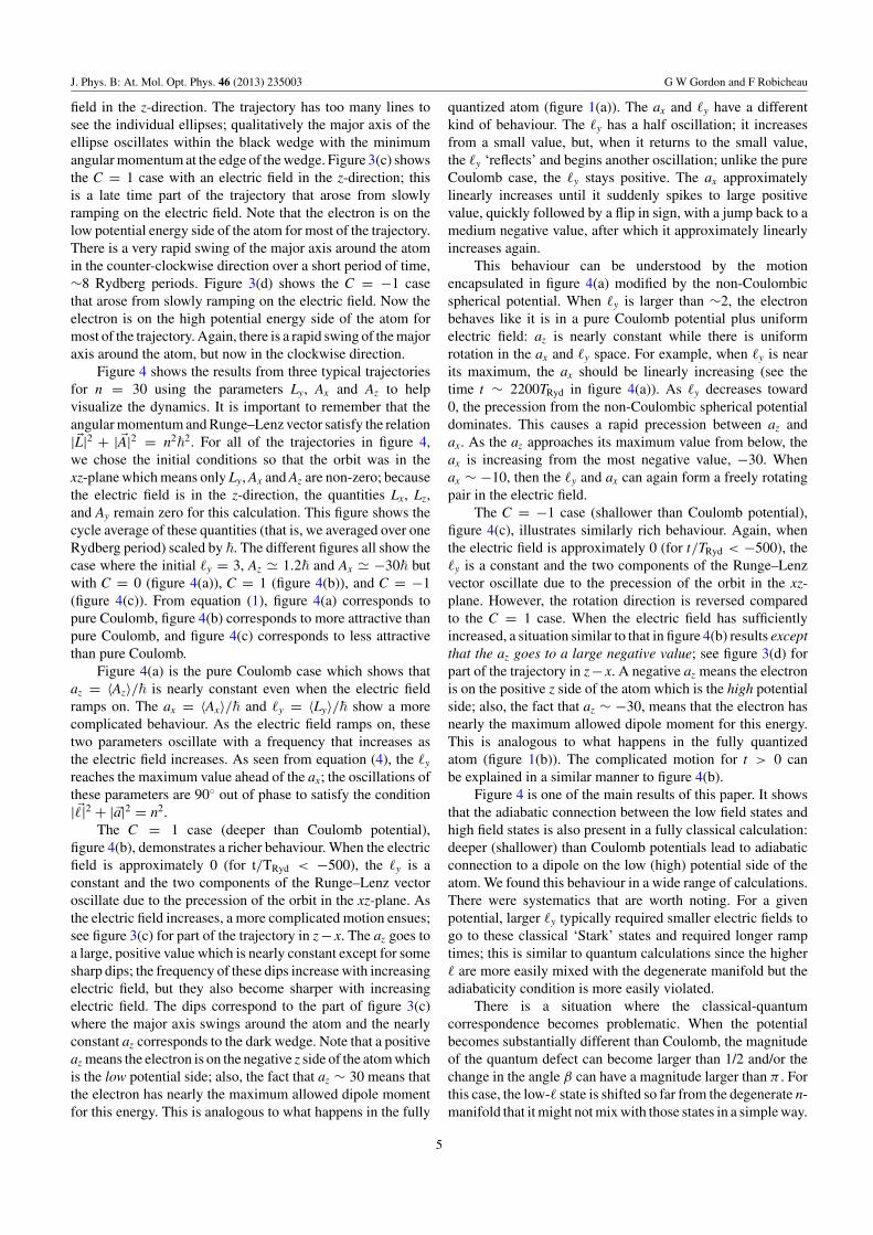
Figure 4 shows the results from three typical trajectoriesfor n = 30 using the parameters Ly, Ax and Az to helpvisualize the dynamics. It is important to remember that theangular momentum and Runge–Lenz vector satisfy the relation|�L|2 + |�A|2 = n2

�2. For all of the trajectories in figure 4,

we chose the initial conditions so that the orbit was in thexz-plane which means only Ly, Ax and Az are non-zero; becausethe electric field is in the z-direction, the quantities Lx, Lz,and Ay remain zero for this calculation. This figure shows thecycle average of these quantities (that is, we averaged over oneRydberg period) scaled by �. The different figures all show thecase where the initial �y = 3, Az � 1.2� and Ax � −30� butwith C = 0 (figure 4(a)), C = 1 (figure 4(b)), and C = −1(figure 4(c)). From equation (1), figure 4(a) corresponds topure Coulomb, figure 4(b) corresponds to more attractive thanpure Coulomb, and figure 4(c) corresponds to less attractivethan pure Coulomb.

Figure 4(a) is the pure Coulomb case which shows thataz = 〈Az〉/� is nearly constant even when the electric fieldramps on. The ax = 〈Ax〉/� and �y = 〈Ly〉/� show a morecomplicated behaviour. As the electric field ramps on, thesetwo parameters oscillate with a frequency that increases asthe electric field increases. As seen from equation (4), the �y

reaches the maximum value ahead of the ax; the oscillations ofthese parameters are 90◦ out of phase to satisfy the condition|��|2 + |�a|2 = n2.

The C = 1 case (deeper than Coulomb potential),figure 4(b), demonstrates a richer behaviour. When the electricfield is approximately 0 (for t/TRyd < −500), the �y is aconstant and the two components of the Runge–Lenz vectoroscillate due to the precession of the orbit in the xz-plane. Asthe electric field increases, a more complicated motion ensues;see figure 3(c) for part of the trajectory in z − x. The az goes toa large, positive value which is nearly constant except for somesharp dips; the frequency of these dips increase with increasingelectric field, but they also become sharper with increasingelectric field. The dips correspond to the part of figure 3(c)where the major axis swings around the atom and the nearlyconstant az corresponds to the dark wedge. Note that a positiveaz means the electron is on the negative z side of the atom whichis the low potential side; also, the fact that az ∼ 30 means thatthe electron has nearly the maximum allowed dipole momentfor this energy. This is analogous to what happens in the fully

quantized atom (figure 1(a)). The ax and �y have a differentkind of behaviour. The �y has a half oscillation; it increasesfrom a small value, but, when it returns to the small value,the �y ‘reflects’ and begins another oscillation; unlike the pureCoulomb case, the �y stays positive. The ax approximatelylinearly increases until it suddenly spikes to large positivevalue, quickly followed by a flip in sign, with a jump back to amedium negative value, after which it approximately linearlyincreases again.

This behaviour can be understood by the motionencapsulated in figure 4(a) modified by the non-Coulombicspherical potential. When �y is larger than ∼2, the electronbehaves like it is in a pure Coulomb potential plus uniformelectric field: az is nearly constant while there is uniformrotation in the ax and �y space. For example, when �y is nearits maximum, the ax should be linearly increasing (see thetime t ∼ 2200TRyd in figure 4(a)). As �y decreases toward0, the precession from the non-Coulombic spherical potentialdominates. This causes a rapid precession between az andax. As the az approaches its maximum value from below, theax is increasing from the most negative value, −30. Whenax ∼ −10, then the �y and ax can again form a freely rotatingpair in the electric field.

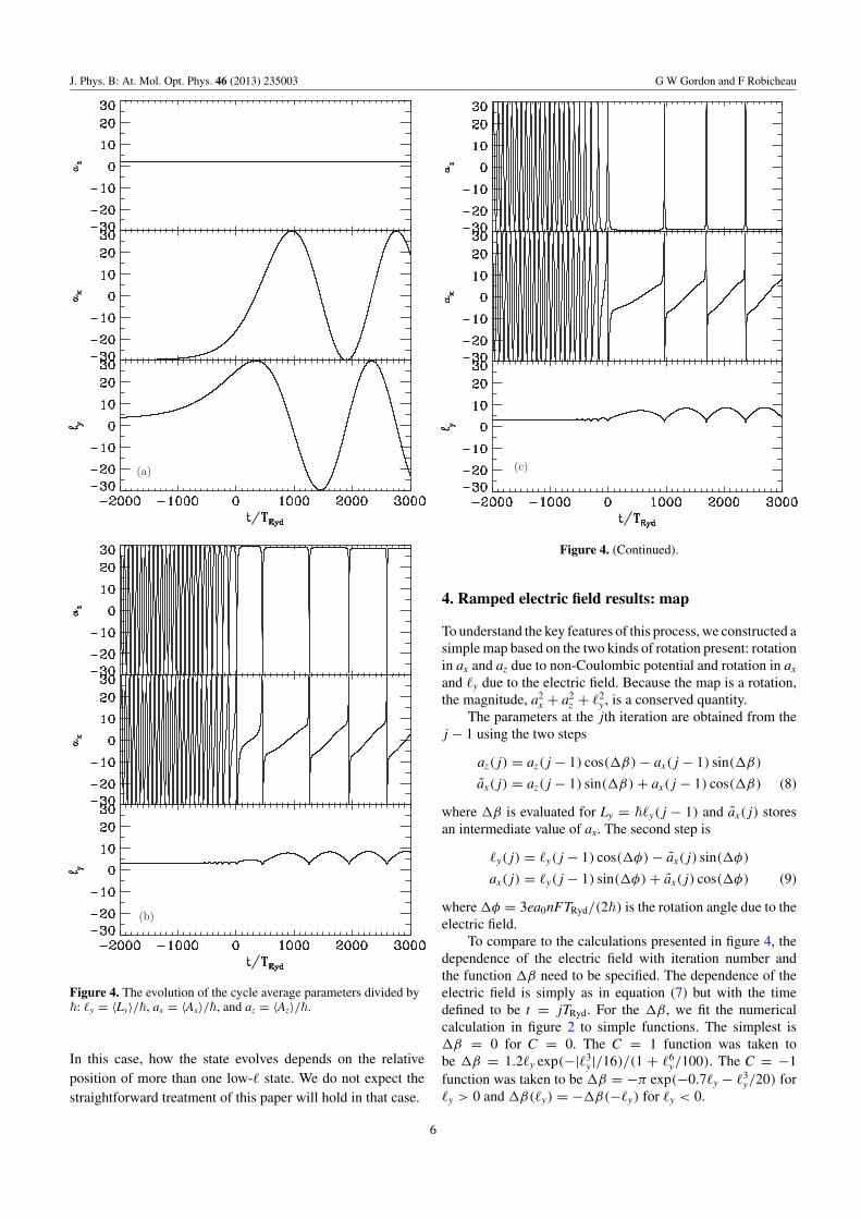
The C = −1 case (shallower than Coulomb potential),figure 4(c), illustrates similarly rich behaviour. Again, whenthe electric field is approximately 0 (for t/TRyd < −500), the�y is a constant and the two components of the Runge–Lenzvector oscillate due to the precession of the orbit in the xz-plane. However, the rotation direction is reversed comparedto the C = 1 case. When the electric field has sufficientlyincreased, a situation similar to that in figure 4(b) results exceptthat the az goes to a large negative value; see figure 3(d) forpart of the trajectory in z− x. A negative az means the electronis on the positive z side of the atom which is the high potentialside; also, the fact that az ∼ −30, means that the electron hasnearly the maximum allowed dipole moment for this energy.This is analogous to what happens in the fully quantizedatom (figure 1(b)). The complicated motion for t > 0 canbe explained in a similar manner to figure 4(b).

Figure 4 is one of the main results of this paper. It showsthat the adiabatic connection between the low field states andhigh field states is also present in a fully classical calculation:deeper (shallower) than Coulomb potentials lead to adiabaticconnection to a dipole on the low (high) potential side of theatom. We found this behaviour in a wide range of calculations.There were systematics that are worth noting. For a givenpotential, larger �y typically required smaller electric fields togo to these classical ‘Stark’ states and required longer ramptimes; this is similar to quantum calculations since the higher� are more easily mixed with the degenerate manifold but theadiabaticity condition is more easily violated.

There is a situation where the classical-quantumcorrespondence becomes problematic. When the potentialbecomes substantially different than Coulomb, the magnitudeof the quantum defect can become larger than 1/2 and/or thechange in the angle β can have a magnitude larger than π . Forthis case, the low-� state is shifted so far from the degenerate n-manifold that it might not mix with those states in a simple way.

5

J. Phys. B: At. Mol. Opt. Phys. 46 (2013) 235003 G W Gordon and F Robicheau

(a)

(b)

Figure 4. The evolution of the cycle average parameters divided by�: �y = 〈Ly〉/�, ax = 〈Ax〉/�, and az = 〈Az〉/�.

In this case, how the state evolves depends on the relativeposition of more than one low-� state. We do not expect thestraightforward treatment of this paper will hold in that case.

(c)

Figure 4. (Continued).

4. Ramped electric field results: map

To understand the key features of this process, we constructed asimple map based on the two kinds of rotation present: rotationin ax and az due to non-Coulombic potential and rotation in ax

and �y due to the electric field. Because the map is a rotation,the magnitude, a2

x + a2z + �2

y , is a conserved quantity.The parameters at the jth iteration are obtained from the

j − 1 using the two steps

az( j) = az( j − 1) cos(�β) − ax( j − 1) sin(�β)

ax( j) = az( j − 1) sin(�β) + ax( j − 1) cos(�β) (8)

where �β is evaluated for Ly = ��y( j − 1) and ax( j) storesan intermediate value of ax. The second step is

�y( j) = �y( j − 1) cos(�φ) − ax( j) sin(�φ)

ax( j) = �y( j − 1) sin(�φ) + ax( j) cos(�φ) (9)

where �φ = 3ea0nFTRyd/(2�) is the rotation angle due to theelectric field.

To compare to the calculations presented in figure 4, thedependence of the electric field with iteration number andthe function �β need to be specified. The dependence of theelectric field is simply as in equation (7) but with the timedefined to be t = jTRyd. For the �β, we fit the numericalcalculation in figure 2 to simple functions. The simplest is�β = 0 for C = 0. The C = 1 function was taken tobe �β = 1.2�y exp(−|�3

y |/16)/(1 + �6y/100). The C = −1

function was taken to be �β = −π exp(−0.7�y − �3y/20) for

�y > 0 and �β(�y) = −�β(−�y) for �y < 0.

6

J. Phys. B: At. Mol. Opt. Phys. 46 (2013) 235003 G W Gordon and F Robicheau

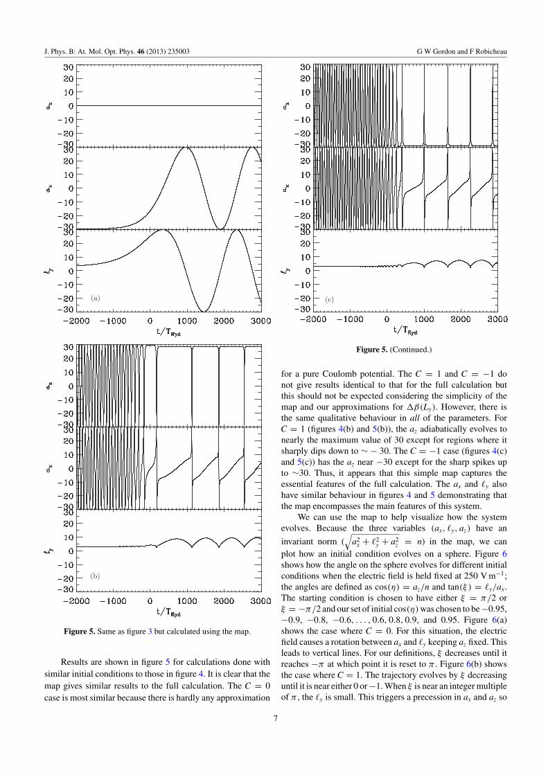
(a)

(b)

Figure 5. Same as figure 3 but calculated using the map.

Results are shown in figure 5 for calculations done withsimilar initial conditions to those in figure 4. It is clear that themap gives similar results to the full calculation. The C = 0case is most similar because there is hardly any approximation

(c)

Figure 5. (Continued.)

for a pure Coulomb potential. The C = 1 and C = −1 donot give results identical to that for the full calculation butthis should not be expected considering the simplicity of themap and our approximations for �β(Ly). However, there isthe same qualitative behaviour in all of the parameters. ForC = 1 (figures 4(b) and 5(b)), the az adiabatically evolves tonearly the maximum value of 30 except for regions where itsharply dips down to ∼ − 30. The C = −1 case (figures 4(c)and 5(c)) has the az near −30 except for the sharp spikes upto ∼30. Thus, it appears that this simple map captures theessential features of the full calculation. The ax and �y alsohave similar behaviour in figures 4 and 5 demonstrating thatthe map encompasses the main features of this system.

We can use the map to help visualize how the systemevolves. Because the three variables (ax, �y, az) have an

invariant norm (√

a2x + �2

y + a2z = n) in the map, we can

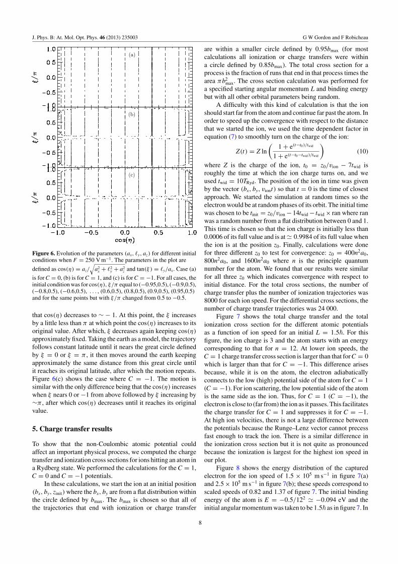
plot how an initial condition evolves on a sphere. Figure 6shows how the angle on the sphere evolves for different initialconditions when the electric field is held fixed at 250 V m−1;the angles are defined as cos(η) = az/n and tan(ξ ) = �y/ax.The starting condition is chosen to have either ξ = π/2 orξ = −π/2 and our set of initial cos(η) was chosen to be −0.95,−0.9, −0.8, −0.6, . . . , 0.6, 0.8, 0.9, and 0.95. Figure 6(a)shows the case where C = 0. For this situation, the electricfield causes a rotation between ax and �y keeping az fixed. Thisleads to vertical lines. For our definitions, ξ decreases until itreaches −π at which point it is reset to π . Figure 6(b) showsthe case where C = 1. The trajectory evolves by ξ decreasinguntil it is near either 0 or −1. When ξ is near an integer multipleof π , the �y is small. This triggers a precession in ax and az so

7

J. Phys. B: At. Mol. Opt. Phys. 46 (2013) 235003 G W Gordon and F Robicheau

(a)

(b)

(c)

Figure 6. Evolution of the parameters (ax, �y, az) for different initialconditions when F = 250 V m−1. The parameters in the plot are

defined as cos(η) = az/√

a2x + �2

y + a2z and tan(ξ ) = �y/ax. Case (a)

is for C = 0, (b) is for C = 1, and (c) is for C = −1. For all cases, theinitial condition was for cos(η), ξ/π equal to (−0.95,0.5), (−0.9,0.5),(−0.8,0.5), (−0.6,0.5), . . . , (0.6,0.5), (0.8,0.5), (0.9,0.5), (0.95,0.5)and for the same points but with ξ/π changed from 0.5 to −0.5.

that cos(η) decreases to ∼ − 1. At this point, the ξ increasesby a little less than π at which point the cos(η) increases to itsoriginal value. After which, ξ decreases again keeping cos(η)

approximately fixed. Taking the earth as a model, the trajectoryfollows constant latitude until it nears the great circle definedby ξ = 0 or ξ = π , it then moves around the earth keepingapproximately the same distance from this great circle untilit reaches its original latitude, after which the motion repeats.Figure 6(c) shows the case where C = −1. The motion issimilar with the only difference being that the cos(η) increaseswhen ξ nears 0 or −1 from above followed by ξ increasing by∼π , after which cos(η) decreases until it reaches its originalvalue.

5. Charge transfer results

To show that the non-Coulombic atomic potential couldaffect an important physical process, we computed the chargetransfer and ionization cross sections for ions hitting an atom ina Rydberg state. We performed the calculations for the C = 1,C = 0 and C = −1 potentials.

In these calculations, we start the ion at an initial position(bx, by, zinit) where the bx, by are from a flat distribution withinthe circle defined by bmax. The bmax is chosen so that all ofthe trajectories that end with ionization or charge transfer

are within a smaller circle defined by 0.95bmax (for mostcalculations all ionization or charge transfers were withina circle defined by 0.85bmax). The total cross section for aprocess is the fraction of runs that end in that process times thearea πb2

max. The cross section calculation was performed fora specified starting angular momentum L and binding energybut with all other orbital parameters being random.

A difficulty with this kind of calculation is that the ionshould start far from the atom and continue far past the atom. Inorder to speed up the convergence with respect to the distancethat we started the ion, we used the time dependent factor inequation (7) to smoothly turn on the charge of the ion:

Z(t) = Z ln

(1 + e(t−t0 )/twid

1 + e(t−t0−twid)/twid

)(10)

where Z is the charge of the ion, t0 = z0/vion − 7twid isroughly the time at which the ion charge turns on, and weused twid = 10TRyd. The position of the ion in time was givenby the vector (bx, by, viont) so that t = 0 is the time of closestapproach. We started the simulation at random times so theelectron would be at random phases of its orbit. The initial timewas chosen to be tinit = z0/vion − 14twid − twid × ran where ranwas a random number from a flat distribution between 0 and 1.This time is chosen so that the ion charge is initially less than0.0006 of its full value and is at � 0.9984 of its full value whenthe ion is at the position z0. Finally, calculations were donefor three different z0 to test for convergence: z0 = 400n2a0,800n2a0, and 1600n2a0 where n is the principle quantumnumber for the atom. We found that our results were similarfor all three z0 which indicates convergence with respect toinitial distance. For the total cross sections, the number ofcharge transfer plus the number of ionization trajectories was8000 for each ion speed. For the differential cross sections, thenumber of charge transfer trajectories was 24 000.

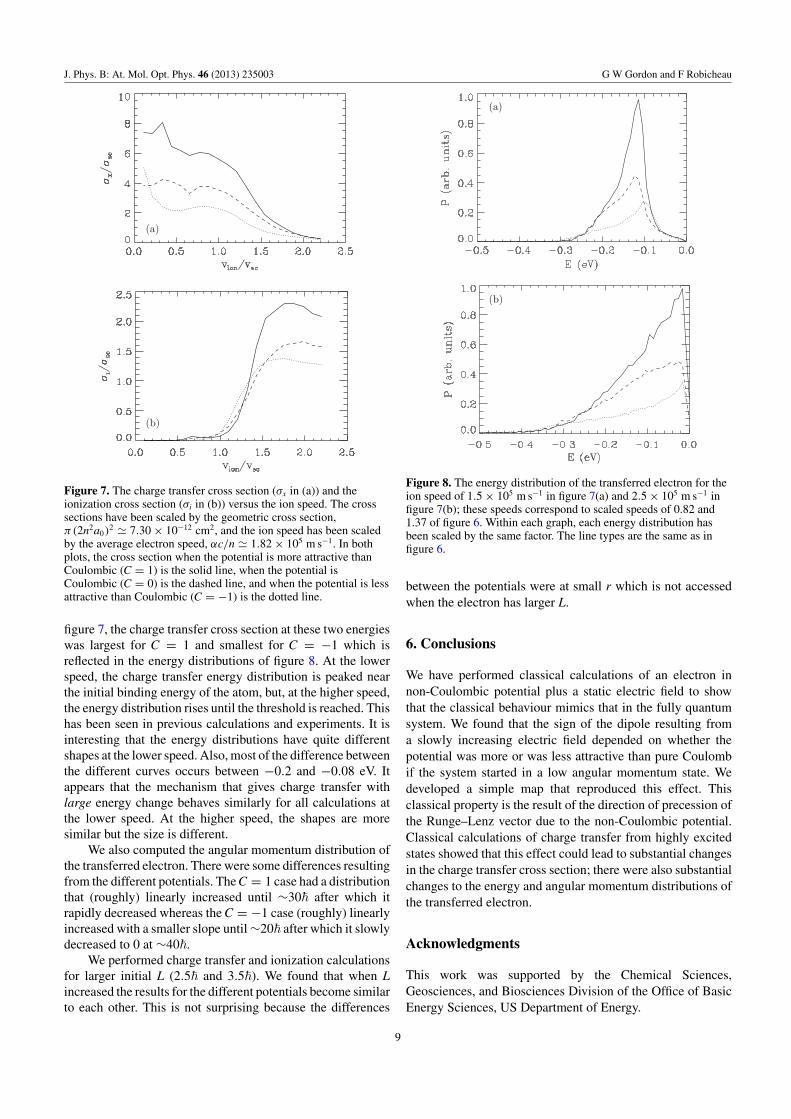
Figure 7 shows the total charge transfer and the totalionization cross section for the different atomic potentialsas a function of ion speed for an initial L = 1.5�. For thisfigure, the ion charge is 3 and the atom starts with an energycorresponding to that for n = 12. At lower ion speeds, theC = 1 charge transfer cross section is larger than that forC = 0which is larger than that for C = −1. This difference arisesbecause, while it is on the atom, the electron adiabaticallyconnects to the low (high) potential side of the atom for C = 1(C = −1). For ion scattering, the low potential side of the atomis the same side as the ion. Thus, for C = 1 (C = −1), theelectron is close to (far from) the ion as it passes. This facilitatesthe charge transfer for C = 1 and suppresses it for C = −1.At high ion velocities, there is not a large difference betweenthe potentials because the Runge–Lenz vector cannot precessfast enough to track the ion. There is a similar difference inthe ionization cross section but it is not quite as pronouncedbecause the ionization is largest for the highest ion speed inour plot.

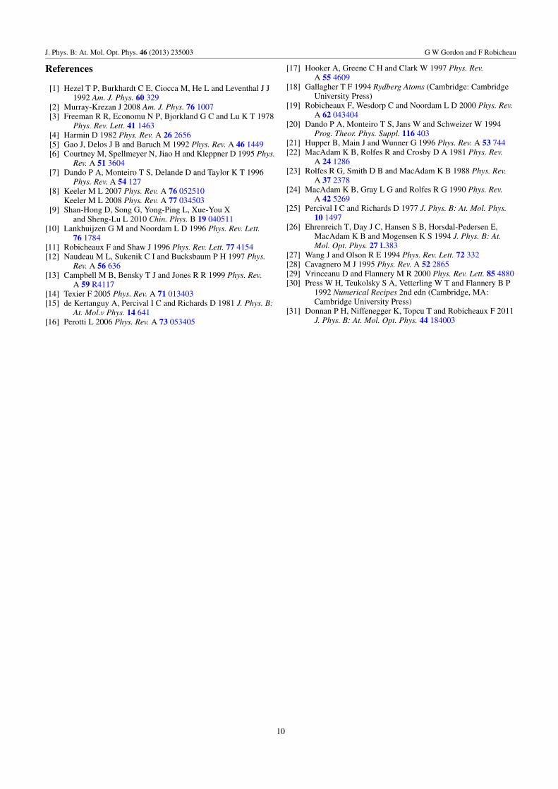
Figure 8 shows the energy distribution of the capturedelectron for the ion speed of 1.5 × 105 m s−1 in figure 7(a)and 2.5 × 105 m s−1 in figure 7(b); these speeds correspond toscaled speeds of 0.82 and 1.37 of figure 7. The initial bindingenergy of the atom is E = −0.5/122 � −0.094 eV and theinitial angular momentum was taken to be 1.5� as in figure 7. In

8

J. Phys. B: At. Mol. Opt. Phys. 46 (2013) 235003 G W Gordon and F Robicheau

(a)

(b)

Figure 7. The charge transfer cross section (σx in (a)) and theionization cross section (σi in (b)) versus the ion speed. The crosssections have been scaled by the geometric cross section,π(2n2a0)

2 � 7.30 × 10−12 cm2, and the ion speed has been scaledby the average electron speed, αc/n � 1.82 × 105 m s−1. In bothplots, the cross section when the potential is more attractive thanCoulombic (C = 1) is the solid line, when the potential isCoulombic (C = 0) is the dashed line, and when the potential is lessattractive than Coulombic (C = −1) is the dotted line.

figure 7, the charge transfer cross section at these two energieswas largest for C = 1 and smallest for C = −1 which isreflected in the energy distributions of figure 8. At the lowerspeed, the charge transfer energy distribution is peaked nearthe initial binding energy of the atom, but, at the higher speed,the energy distribution rises until the threshold is reached. Thishas been seen in previous calculations and experiments. It isinteresting that the energy distributions have quite differentshapes at the lower speed. Also, most of the difference betweenthe different curves occurs between −0.2 and −0.08 eV. Itappears that the mechanism that gives charge transfer withlarge energy change behaves similarly for all calculations atthe lower speed. At the higher speed, the shapes are moresimilar but the size is different.

We also computed the angular momentum distribution ofthe transferred electron. There were some differences resultingfrom the different potentials. The C = 1 case had a distributionthat (roughly) linearly increased until ∼30� after which itrapidly decreased whereas the C = −1 case (roughly) linearlyincreased with a smaller slope until ∼20� after which it slowlydecreased to 0 at ∼40�.

We performed charge transfer and ionization calculationsfor larger initial L (2.5� and 3.5�). We found that when Lincreased the results for the different potentials become similarto each other. This is not surprising because the differences

(a)

(b)

Figure 8. The energy distribution of the transferred electron for theion speed of 1.5 × 105 m s−1 in figure 7(a) and 2.5 × 105 m s−1 infigure 7(b); these speeds correspond to scaled speeds of 0.82 and1.37 of figure 6. Within each graph, each energy distribution hasbeen scaled by the same factor. The line types are the same as infigure 6.

between the potentials were at small r which is not accessedwhen the electron has larger L.

6. Conclusions

We have performed classical calculations of an electron innon-Coulombic potential plus a static electric field to showthat the classical behaviour mimics that in the fully quantumsystem. We found that the sign of the dipole resulting froma slowly increasing electric field depended on whether thepotential was more or was less attractive than pure Coulombif the system started in a low angular momentum state. Wedeveloped a simple map that reproduced this effect. Thisclassical property is the result of the direction of precession ofthe Runge–Lenz vector due to the non-Coulombic potential.Classical calculations of charge transfer from highly excitedstates showed that this effect could lead to substantial changesin the charge transfer cross section; there were also substantialchanges to the energy and angular momentum distributions ofthe transferred electron.

Acknowledgments

This work was supported by the Chemical Sciences,Geosciences, and Biosciences Division of the Office of BasicEnergy Sciences, US Department of Energy.

9

J. Phys. B: At. Mol. Opt. Phys. 46 (2013) 235003 G W Gordon and F Robicheau

References

[1] Hezel T P, Burkhardt C E, Ciocca M, He L and Leventhal J J1992 Am. J. Phys. 60 329

[2] Murray-Krezan J 2008 Am. J. Phys. 76 1007[3] Freeman R R, Economu N P, Bjorkland G C and Lu K T 1978

Phys. Rev. Lett. 41 1463[4] Harmin D 1982 Phys. Rev. A 26 2656[5] Gao J, Delos J B and Baruch M 1992 Phys. Rev. A 46 1449[6] Courtney M, Spellmeyer N, Jiao H and Kleppner D 1995 Phys.

Rev. A 51 3604[7] Dando P A, Monteiro T S, Delande D and Taylor K T 1996

Phys. Rev. A 54 127[8] Keeler M L 2007 Phys. Rev. A 76 052510

Keeler M L 2008 Phys. Rev. A 77 034503[9] Shan-Hong D, Song G, Yong-Ping L, Xue-You X

and Sheng-Lu L 2010 Chin. Phys. B 19 040511[10] Lankhuijzen G M and Noordam L D 1996 Phys. Rev. Lett.

76 1784[11] Robicheaux F and Shaw J 1996 Phys. Rev. Lett. 77 4154[12] Naudeau M L, Sukenik C I and Bucksbaum P H 1997 Phys.

Rev. A 56 636[13] Campbell M B, Bensky T J and Jones R R 1999 Phys. Rev.

A 59 R4117[14] Texier F 2005 Phys. Rev. A 71 013403[15] de Kertanguy A, Percival I C and Richards D 1981 J. Phys. B:

At. Mol.v Phys. 14 641[16] Perotti L 2006 Phys. Rev. A 73 053405

[17] Hooker A, Greene C H and Clark W 1997 Phys. Rev.A 55 4609

[18] Gallagher T F 1994 Rydberg Atoms (Cambridge: CambridgeUniversity Press)

[19] Robicheaux F, Wesdorp C and Noordam L D 2000 Phys. Rev.A 62 043404

[20] Dando P A, Monteiro T S, Jans W and Schweizer W 1994Prog. Theor. Phys. Suppl. 116 403

[21] Hupper B, Main J and Wunner G 1996 Phys. Rev. A 53 744[22] MacAdam K B, Rolfes R and Crosby D A 1981 Phys. Rev.

A 24 1286[23] Rolfes R G, Smith D B and MacAdam K B 1988 Phys. Rev.

A 37 2378[24] MacAdam K B, Gray L G and Rolfes R G 1990 Phys. Rev.

A 42 5269[25] Percival I C and Richards D 1977 J. Phys. B: At. Mol. Phys.

10 1497[26] Ehrenreich T, Day J C, Hansen S B, Horsdal-Pedersen E,

MacAdam K B and Mogensen K S 1994 J. Phys. B: At.Mol. Opt. Phys. 27 L383

[27] Wang J and Olson R E 1994 Phys. Rev. Lett. 72 332[28] Cavagnero M J 1995 Phys. Rev. A 52 2865[29] Vrinceanu D and Flannery M R 2000 Phys. Rev. Lett. 85 4880[30] Press W H, Teukolsky S A, Vetterling W T and Flannery B P

1992 Numerical Recipes 2nd edn (Cambridge, MA:Cambridge University Press)

[31] Donnan P H, Niffenegger K, Topcu T and Robicheaux F 2011J. Phys. B: At. Mol. Opt. Phys. 44 184003

10