A COARSENING ALGORITHM ON ADAPTIVE GRIDS BYNEWEST VERTEX BISECTION AND ITS APPLICATIONS

Long Chen

Department of Mathematics, University of California at Irvine, Irvine, CA 92697

Email: chenlong@math.uci.edu

Chen-Song Zhang

Department of Mathematics, The Pennsylvania State University, University Park, PA, 16802

Email: zhangcs@psu.edu

Abstract

In this paper, an efficient and easy-to-implement coarsening algorithm is proposed for

adaptive grids obtained using the newest vertex bisection method in R2. The coarsen-

ing algorithm does not require storing the binary refinement tree explicitly. Instead, the

structure is implicitly contained in a special ordering of triangular elements. Numerical

experiments demonstrate that the proposed coarsening algorithm is very efficient when

applied for multilevel preconditioners and mesh adaptivity for time-dependent problems.

Mathematics subject classification: 65M55, 65N55, 65N22, 65F10.

Key words: adaptive finite element method, coarsening, newest vertex bisection, multilevel

preconditioning

1. Introduction

Adaptive methods are now widely employed in the scientific computation to achieve betteraccuracy with minimum degree of freedom. A typical adaptive finite element method throughlocal refinement can be written as the following loop:

SOLVE→ ESTIMATE→MARK→ REFINE/COARSEN. (1.1)

In this paper, we shall consider the modules COARSEN and SOLVE. More precisely, wepropose a new efficient and easy-to-implement coarsening algorithm and apply to multilevelpreconditioners for adaptive grids obtained by the newest vertex bisection in two spatial di-mensions.

Classical recursive bisection and coarsening algorithms [21] are widely used in adaptivealgorithms (see, for example, ALBERTA [31] and deal.II [3]). These algorithms make use ofbinary-tree related data structures and subroutines to store and access the bisection history.

We propose a new node-wise coarsening algorithm which does not require storing the bisec-tion tree explicitly. We only store coordinates of vertices and connectivity of triangles whichis the minimal information to represent a mesh for standard finite element computation. Wecan built a kind of tree structure into a special ordering of the triangles. By doing this way, wesimplify the implementation of adaptive mesh refinement and coarsening and thus provide aneasy-access interface for the usage of mesh adaptation without too much sacrifice in time.

The coarsening algorithm can be applied to construct efficient multilevel solvers for ellipticproblems. Based on the special geometric relation between nested triangulations obtained by

http://www.global-sci.org/jcm Global Science Preprint

2

our coarsening algorithm, we develop a new multilevel preconditioner which numerically out-performs several classical multilevel preconditioners.

The proposed coarsening algorithm can also be employed for mesh adaptation, especially fortime-dependent problems. For steady-state problems, quasi-optimal meshes can be obtained inpractice using (1.1) without the COARSEN step [11]. However, it is not the case for time-dependent problems as the local features might change dramatically in time. We provide anumerical example for the application of our coarsening algorithm to time-dependent problems.

The rest of the paper is organized as follows. We review the classical coarsening algorithmand introduce our new algorithm in Section 2. We explain the data structures and implemen-tation of our coarsening algorithm in Section 3. In order to demonstrate the performance ofthe proposed coarsening algorithm, then we show two applications of our coarsening algorithm:one is multilevel preconditioners for stationary problems in Section 4 and the other is meshadaptation for time-dependent problems in Section 5.

2. Coarsening Algorithms

In this section, we a the new coarsening algorithm for triangular meshes obtained by thenewest vertex bisection method. Unlike the classical recursive coarsening algorithm, the pro-posed algorithm is non-recursive and requires neither storing nor maintaining the bisection treeinformation such as the parents, brothers, generation, etc.

2.1. Conformity and shape-regularity of triangulations

Let Ω ⊂ R2 be a polygonal domain. A triangulation T (also known as mesh or grid) of Ω isa set of triangles (also indicated by elements) which is a partition of Ω. The set of nodes (alsoindicated by vertices or points) of the triangulation T is denoted by N (T ) and the set of alledges by E(T ). As a convention, all triangles t ∈ T and edges e ∈ E(T ) are closed sets.

We define the first ring of a point p ∈ Ω or an edge e ∈ E(T ) as

Rp := t ∈ T | p ∈ t and Re := t ∈ T | e ⊂ t,

respectively; and define the local patch of p or e as

ωp :=⋃

t∈Rp

t and ωe :=⋃

t∈Re

t,

respectively. Note that ωp and ωe are subdomains of Ω ⊂ R2, while Rp and Re are sets oftriangles which can be viewed as triangulations of ωp and ωe, respectively. The cardinality of aset S is denoted by #S. For each vertex p ∈ N (T ), the valence of p is defined as the numberof triangles in Rp, i.e., #Rp.

For finite element discretizations, there are two standard conditions imposed on triangula-tions. The first condition is the conformity. A triangulation T is conforming if the intersectionof any two triangles t1 and t2 in T either consists of a common vertex, a common edge, or empty.The second condition is the shape-regularity. A set of triangulations F is called shape-regularif there exists a constant σ such that

maxt∈T

diam(t)|t| 12

≤ σ, for all T ∈ F , (2.1)

where diam(t) is the diameter of t and |t| is the area of t.

3

2.2. Newest vertex bisection

We review the newest vertex bisection method studied in detail by Mitchell [24, 25]. Morerecent study on newest vertex bisection can be found in Binev, DeVore and Dahmen [8]. Ashort implementation of such bisection method in MATLAB can be found in [12]; see also [13].

For each triangle t ∈ T , we label one vertex of t as the newest vertex and call it V (t). Theopposite edge of V (t) is called the refinement edge and denoted by E(t). This process is calleda labeling of T . Starting with a labeled initial grid T0, newest vertex bisection follows two rules:

1. a triangle (father) is bisected to obtain two new triangles (children) by connecting itsnewest vertex with the midpoint of its refinement edge;

2. the new vertex created at the midpoint of the refinement edge is labeled as the newestvertex of each child.

Once the labeling is done for an initial grid, the decent grids inherit labels according to thesecond rule and the bisection process can thus proceed.

For a given labeled initial grid T0, we define

F(T0) := T | T is obtained from T0 by newest vertex bisection(s). (2.2)

Sewell [32] showed that all the descendants of a triangle in T0 fall into four similarity classesand hence any triangulation T ∈ F(T0) is shape-regular. It is worth to note that T ∈ F(T0) isnot necessarily conforming. Therefore we define a subset of F(T0):

C(T0) := T ∈ F(T0) | T is conforming. (2.3)

We now give an example to illustrate the bisection procedure above and address the con-formity issue. To begin with, we introduce some notation. The generation of each triangle inthe initial grid is defined to be 0; once a triangle is bisected, the generations of both childrenare defined as one plus the generation of their father. The generation of a triangle t ∈ T willbe denoted by g(t). Children with the same father are called brothers to each other.

T0

T1

T2

T3

t0,1

t1,1 t1,2

t2,1 t2,2

t3,1 t3,2

t2,3 t2,4

t3,3 t3,4

1

Fig. 2.1. Bisection tree (left) and its corresponding grids (right).

In Figure 2.1, we start from an initial grid T0 with only one triangle t0,1. In the notationti,j , the first subscript i is the generation of the triangle and the second subscript j is the index

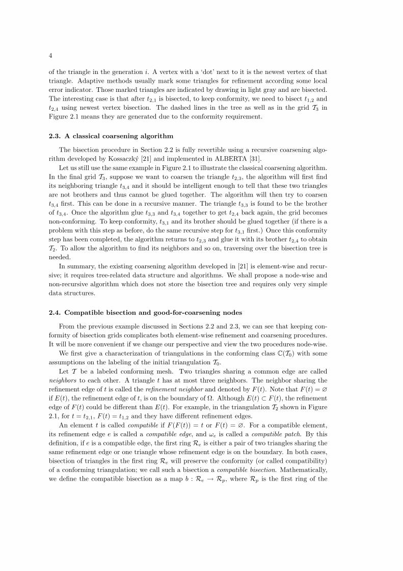
4

of the triangle in the generation i. A vertex with a ‘dot’ next to it is the newest vertex of thattriangle. Adaptive methods usually mark some triangles for refinement according some localerror indicator. Those marked triangles are indicated by drawing in light gray and are bisected.The interesting case is that after t2,1 is bisected, to keep conformity, we need to bisect t1,2 andt2,4 using newest vertex bisection. The dashed lines in the tree as well as in the grid T3 inFigure 2.1 means they are generated due to the conformity requirement.

2.3. A classical coarsening algorithm

The bisection procedure in Section 2.2 is fully revertible using a recursive coarsening algo-rithm developed by Kossaczky [21] and implemented in ALBERTA [31].

Let us still use the same example in Figure 2.1 to illustrate the classical coarsening algorithm.In the final grid T3, suppose we want to coarsen the triangle t2,3, the algorithm will first findits neighboring triangle t3,4 and it should be intelligent enough to tell that these two trianglesare not brothers and thus cannot be glued together. The algorithm will then try to coarsent3,4 first. This can be done in a recursive manner. The triangle t3,3 is found to be the brotherof t3,4. Once the algorithm glue t3,3 and t3,4 together to get t2,4 back again, the grid becomesnon-conforming. To keep conformity, t3,1 and its brother should be glued together (if there is aproblem with this step as before, do the same recursive step for t3,1 first.) Once this conformitystep has been completed, the algorithm returns to t2,3 and glue it with its brother t2,4 to obtainT2. To allow the algorithm to find its neighbors and so on, traversing over the bisection tree isneeded.

In summary, the existing coarsening algorithm developed in [21] is element-wise and recur-sive; it requires tree-related data structure and algorithms. We shall propose a node-wise andnon-recursive algorithm which does not store the bisection tree and requires only very simpledata structures.

2.4. Compatible bisection and good-for-coarsening nodes

From the previous example discussed in Sections 2.2 and 2.3, we can see that keeping con-formity of bisection grids complicates both element-wise refinement and coarsening procedures.It will be more convenient if we change our perspective and view the two procedures node-wise.

We first give a characterization of triangulations in the conforming class C(T0) with someassumptions on the labeling of the initial triangulation T0.

Let T be a labeled conforming mesh. Two triangles sharing a common edge are calledneighbors to each other. A triangle t has at most three neighbors. The neighbor sharing therefinement edge of t is called the refinement neighbor and denoted by F (t). Note that F (t) = ∅if E(t), the refinement edge of t, is on the boundary of Ω. Although E(t) ⊂ F (t), the refinementedge of F (t) could be different than E(t). For example, in the triangulation T2 shown in Figure2.1, for t = t2,1, F (t) = t1,2 and they have different refinement edges.

An element t is called compatible if F (F (t)) = t or F (t) = ∅. For a compatible element,its refinement edge e is called a compatible edge, and ωe is called a compatible patch. By thisdefinition, if e is a compatible edge, the first ring Re is either a pair of two triangles sharing thesame refinement edge or one triangle whose refinement edge is on the boundary. In both cases,bisection of triangles in the first ring Re will preserve the conformity (or called compatibility)of a conforming triangulation; we call such a bisection a compatible bisection. Mathematically,we define the compatible bisection as a map b : Re → Rp, where Rp is the first ring of the

5

new point p introduced in the bisection. We note that the inverse map b−1 : Rp → Re can bethought as a coarsening step. It is restricted to the local patch ωp and thus no conformity issuearises. See Figure 2.2 for an illustration. In this figure, the edges in boldface are the refinementedges and dash-lines represent bisections.

example, in the triangulation T2 shown in Figure ??, for t = t2,1, F (t) = t1,2 and they have

different refinement edges.

eb

b!1p e

b

b!1p

FIG. 2.2. Two compatible bisections. Left: interior edge; right: boundary edge. The vertex near the dot is the

newest vertex, the edge with boldface is the refinement edge, and the dash-line represents the bisection.

An element t is called compatible if F (t) = ! or F (F (t)) = t, i.e. E(t) = E(t"). Fora compatible element, its refinement edge e is called a compatible edge, and !e is called a

compatible patch. By the definition, the first ring Re is a pair of two triangles sharing the

same refinement edge e or a triangle whose refinement edge e is on the boundary. In either

case, bisecting every element in the first ringRe gives a new conforming triangulation. We

shall call it a compatible bisection. More precisely, we define the compatible bisection as a

map

b : Re ! Rx.

We note that the inverse map of b i.e.

b!1 : Rx ! Re,

can be thought as a coarsening process. It is restricted to the local patch !x and thus no

conformity issue arises. See Figure ?? for an illustration. The question is how to find the

node introduced by a compatible bisection without recording b explicitly. To this end, we

shall introduce the following concept.

DEFINITION 2.1 (Good-for-coarsening Nodes). For a triangulation T " T(T0), a nodex " N (T ) is called a good-for-coarsening node, or a good node in short, if there exist acompatible bisection b and compatible patchRe such thatRx = b(Re). The set of all goodnodes in the grid T will be denoted by G(T ).

The first question is whether there exist good nodes for a given grid T " T(T0). In gen-eral, G(T ) could be empty; see Figure ?? for such an example. This example indicates thatthe labeling for the initial triangulation cannot be selected freely. We need impose some con-

ditions on the labeling of the initial triangulation. We call a labeled grid T compatible labeled

if every element in T is compatible and call such a labeling of T a compatible labeling.The following theorem proves the existence of good nodes and gives the practical char-

acterization of good nodes if we begin with a labeled compatible triangulation T0. The proof

is rather technical and thus is postponed to the appendix.

THEOREM 2.2 (Existence and Characterization of Good Nodes). Let T0 be a compatible

labeled conforming triangulation. For any T " T(T0) and T #= T0, the set of good nodes

G(T ) is not empty. Furthermore x " G(T ) if and only if1. it is not a vertex of the initial grid T0;

2. it is the newest vertex of all elements inRx.

3. #Rx = 4 for an interior node x or #Rx = 2 for a boundary node x.

5

Fig. 2.2. Two examples of compatible bisections. Left: interior edge; right: boundary edge.

If we have access to all compatible bisections, we can easily perform a node-wise coarsening.The question is how to find the node introduced by a compatible bisection without recordingall compatible bisections. To this end, we introduce a new concept:

Define 1 (Good-for-coarsening Node) For a triangulation T ∈ C(T0), a node p ∈ N (T ) iscalled a good-for-coarsening node, or a good node in short, if there exist a compatible bisectionb and a compatible patch Re such that Rp = b(Re). The set of all good nodes in the grid T isdenoted by G(T ).

2.5. Existence of good nodes on compatibly labeled grids

In general, the set of good nodes G(T ) could be empty; see Figure 2.3 for such an example.This example indicates that the labeling for the initial triangulation cannot be selected freelyand it is necessary to impose some conditions on the initial labeling.

REMARK 2.3. The assumption: T0 is compatible labeled is not restrictive. Indeed

Mitchell [?] proved that for any conforming triangulation T , there exist a compatible la-beling. Recently Biedl, Bose, Demaine, and Lubiw [?] give an O(N) algorithm to find a

compatible labeling for a triangulation with N elements.

REMARK 2.4. The assumption: T0 is compatible labeled could be further relaxed by

using the longest edge of each triangle as its refinement edge for the initial triangulation T0;

see Kossaczky [?].

•

••

•

• •

(a) Non-compatible labeling (b) One bisection on each element (c) Bisections for conformity

FIG. 2.3. Bisections on a non-compatible triangulation

Our new coarsening algorithm is simply read as the following:

Algorithm T ! = COARSENING(T )Find G(T ), all good nodes of T ;Replace Rx by b"1(Rx) for x ! G(T ).

END Algorithm

We shall discuss the implementation of these two abstract steps in the next section. Here

we continue theoretical questions on the coarsening algorithm. An important one is whether

we can finally obtain the initial grid back by applying this coarsening algorithm iteratively.

The answer is positive and a rigorous discussion is given in the following theorem.

THEOREM 2.5 (Coarsening Theorem). Let T0 be a compatible labeled conforming tri-

angulation. For any T ! T(T0), there exists a positive integer L < " such that by applying

COARSENING L times iteratively, we obtain T0 back.

Proof. If T = T0, we can simply choose L = 0. When T #= T0, by the existence of

good nodes (Theorem ??), we obtain a new grid T ! = COARSENING(T ) with #N (T !) <

#N (T ).We now prove that T ! ! T(T0) i.e. T ! is also conforming. If x is a boundary node, by

the definition of good nodes, there are only two elements in Rx and they are from the same

father and are brothers to each other. So gluing these two elements into one element results

in a grid still in the class T(T0). On the other hand, if x is an interior point, there are two

pairs of brothers. Since we glue children from the same fathers together, the resulting two

elements share a compatible edge and the resulting grid is also in T(T0).If T ! #= T0, we can continue applying the COARSENING algorithm on T !. Therefore

with at most L = #N (T )$#N (T0) steps, we obtain T0.

REMARK 2.6. In the theorem above, the worst case scenario isL = #N (T )$#N (T0).For multilevel methods, generally there is no need to return to the initial grid T0. Our numer-

ical examples strongly indicates that after a very few number of coarsening steps (about 56

Fig. 2.3. Bisections on a non-compatible triangulation. Left: a non-compatible labeling; middle: one

bisection on each triangle; right: bisections for conformity.

If all elements in T ∈ F(T0) have the same generation k, T is called the k-th uniformrefinement of T0 and is denoted by T k. Note that T k might not be conforming; see Figure 2.3(middle) for example. Let P(T0) = ∪N (T ) : T ∈ F(T0) denote the set of all possible nodes.For any node p ∈ P(T0), we define the generation of p, denoted by g(p), to be the minimalinteger k such that p ∈ N (T k).

We call a grid T compatibly labeled if every element in T is compatible and call such alabeling of T a compatible labeling. The following theorem shows the existence of good nodesand gives a practical characterization of good nodes if the initial grid T0 is compatibly labeled.

6

Theorem 2.1 (Existence and Characterization of Good Nodes) Let T0 be a compatiblylabeled conforming triangulation. For any T ∈ C(T0) and T 6= T0, let

M1(T ) := p ∈ N (T ) : g(p) ≥ 1, g(p) = maxq∈N (Rp)

g(q),

M2(T ) := p ∈ N (T ) : p /∈ N (T0) and p = V (t) ∀t ∈ Rp.

Then G(T ) =M1(T ) =M2(T ) 6= ∅.

Remark 2.1 (Compatible Initial Labeling) The assumption “T0 is compatibly labeled” isnot restrictive. In fact, Mitchell [24] proved that for any conforming triangulation T , thereexists a compatible labeling. Biedl et al. [5] give an O(N) algorithm to find a compatiblelabeling for a triangulation with N elements. This assumption can be further relaxed by usingthe longest edge of each triangle as its refinement edge for the initial triangulation T0; seeKossaczky [21]. Note that such conditions are also needed in the proof of convergence andoptimality of adaptive finite element methods [11].

To prove Theorem 2.1, we first study a property on uniform refinements.

Lemma 2.1 (Uniform Refinements on A Compatible Mesh) If T0 is conforming andcompatibly labeled, then every uniform refinement T k of T0 is also conforming and compati-bly labeled.

Proof. We prove it by induction of k. For k = 0, T0 is conforming and compatibly labeled.Suppose T k−1 is conforming and compatibly labeled, we will show so is T k. Since T k−1 iscompatibly labeled, after bisecting every element of T k−1, we obtain T k which is conforming.We only need to prove T k is also compatibly labeled.

We pick up a triangle t ∈ T k. If F (t) = ∅, t is compatible by definition. We now considerthe case F (t) 6= ∅. Denoted by the father of a triangle t by father(t). Since t is refined

! = (!1, 1)2, f = 1 and g = 0. In this example, we keep a1 = 1 and change a2 from 1to 104 on the same grid (uniform refinement by newest bisection). From iteration numbers

listed in Table 5.5, we can see that the new preconditioner is not sensitive to the size of jumps.

DOF 961 1985 3969 8065 16129

a2 = 1 10 8 9 11 9

a2 = 10 10 9 10 11 10

a2 = 102 10 9 10 11 10

a2 = 103 10 9 10 11 10

a2 = 104 10 9 10 11 10

TABLE 5.5

Number of iterations by PCG (initial guessu0 = 0 and tol = 10!6) with OHB for example 3.

Appendix: Proof of the Existence and Characterization of Good Nodes. We shall

give a proof of the existence and characterization of good nodes (Theorem 2.2) in this section.

To this end, we first introduce the concept of uniform refinement grids.

If all elements in T " F(T0) have the same generation k, T is called the k-th uniform

refinement of T0 and is denoted by T k. In contrast to the regular refinement which connects

midpoints of all edges to divide every element into four triangles, for bisection methods, the

uniform refinement T k is not necessary conforming; see Figure 2.3(b) for such an example.

THEOREM 5.1 (Properties of Uniform Refinement). If T0 is conforming and compatible

labeled, then every uniform refinement T k of T0 is also conforming and compatible labeled.

Proof. We shall prove it by the induction of k. When k = 0, T0 is conforming and

compatible labeled by assumption. Suppose T k!1 is conforming and compatible labeled, we

shall show so is T k. First since T k!1 is compatible labeled, after bisecting every element of

T k!1, we obtain a conforming grid T k.

Now we prove the T k is compatible labeled. Recall that F (t) denotes the triangle (ifany) containing the refinement edge of t. If F (t) = !, by the definition, t is compatible.Otherwise, we need to prove F (F (t)) = t, namely E(t) = e(F (t)).

For any element t " T k, we denote its father by father(t). Since t is refined from its

father, we know E(t) #= E(father(t)). By the same reason, E(F (t)) #= E(father(F (t))).By the conformity of T k!1, we know E(t) is an edge of both father(t) and father(F (t)).After bisection, in T k, E(t) becomes the refinement edge of F (t) and t. See Figure 5.5.

t F (t)

father(t) father(F (t))

FIG. 5.5. Refinement edges of t and F (t).

DEFINITION 5.2 (Generation of nodes). Let N (T0) = $N (T ) : T " F(T0) denotethe set of all possible nodes. For any node x " N (T0), we define the generation of x to be

19

Fig. 2.4. Refinement edges of t and F (t).

from its father, E(t) 6= E(father(t)). By the same reason, E(F (t)) 6= E(father(F (t))). Bythe conformity of T k−1, E(t) is an edge of both father(t) and father(F (t)). In the trianglefather(F (t)), it is evident that after the bisection, the refinement edge of F (t) is also E(t); seeFigure 2.4 for an illustration of one possible configuration of t and F (t).

If we begin with a compatibly labeled initial triangulation T0, then for any p ∈ N (T k) withk = g(p), k ≥ 1, p is introduced by a compatible bisection from T k−1 and thus p must be agood node. More precisely, if we denote the ring of p in T k as Rk,p with k = g(p) and thefirst ring of e ∈ E(T k−1) by Rk−1,e, then be : Rk−1,e → Rk,p is the compatible bisection whichintroduces p.

Remark 2.2 (Generation of Elements) Let T0 be a compatibly labeled triangulation andT ∈ C(T0), but T 6= T0. For any t ∈ T \T0, V (t), the newest vertex of t, is introduced later than

7

other vertices of t and thus g(V (t)) > g(p), for any vertex p of t and p 6= V (t). Since t ∈ T g(t)and t /∈ T k for k < g(t), we conclude that g(t) = g(V (t)).

Now we are at the position to complete the proof of Theorem 2.1.Proof of Theorem 2.1. Let p∗ ∈ N (T ) such that g(p∗) = maxq∈N (T ) g(q). Then p∗ ∈ M1(T )and thus M1(T ) is non-empty.

We then show the equivalence ofM1(T ) andM2(T ). It is obvious that g(p) ≥ 1 is equivalentto p /∈ N (T0). Let us pick up a p ∈ M1(T ). Suppose there is a triangle t ∈ Rp and V (t) 6= p.Then we have g(V (t)) > g(p) which contradicts with the choice of p. So we conclude p is thenewest vertex of all triangles in Rp. On the other hand, if p is the newest vertex of all elementsin Rp, then g(p) = g(V (t)) ≥ g(q) for any t ∈ Rp, q ∈ N (τ), i.e., g(p) will be a local maximumin Rp. This finishes the proof of the equivalence of M1(T ) and M2(T ).

The proof of G(T ) ⊆ M2(T ) is straightforward. Since p is introduced by a compatiblebisection, p should be the newest vertex of all t ∈ Rp.

To complete the proof, we now prove M1(T ) ⊆ G(T ). Let p ∈ M1(T ). For any t ∈ Rp,g(t) = g(V (t)) = g(p) and consequently Rp ⊆ Rk,p. Since ωp is hormophism to a disk (interiornode) or half disk (boundary node) with the center p, we conclude Rp = Rk,p and thus p is agood node.

Remark 2.3 (Characterization in 2-D) In R2, there are only two possibilities for compat-ible bisections, for p ∈ G(T ), #Rp = 4 or #Rp = 2. This characterization will help us to findout all good nodes without recording the generation; see Section 3.2.

Remark 2.4 (Generalization to 3-D) Existence of good nodes (Theorem 2.1) can be easilygeneralized to three or higher dimensions, if we can choose an initial labeling of T0 such thatall uniform refinement T k, k ≥ 1 are conforming. However, we need to record the generation ofnodes and extra information; see [13] for details.

2.6. A node-wise coarsening algorithm

Formally, our new coarsening algorithm simply reads:

ALGORITHM COARSEN (T )Find all good nodes G(T ) of T .For each good node p ∈ G(T )Replace the first ring Rp by b−1

e (Rp).END

We postpone the discussion on implementation of this algorithm to the next section andcontinue theoretical discussions on the coarsening algorithm. An important question is whetherwe can finally obtain the initial grid back by repeatedly applying this coarsening algorithm.The answer is positive and a rigorous discussion is given in the following theorem.

Theorem 2.2 (Coarsening Theorem) Let T0 be a compatibly labeled conforming triangula-tion. For any T ∈ C(T0), there exists a positive integer L ≤ #N (T ) − #N (T0) such that byapplying the algorithm COARSEN at most L times, we can recover T0.

Proof. If T = T0, we can simply choose L = 0. When T 6= T0, by the existence of goodnodes (Theorem 2.1), we obtain a new grid T ′ =COARSEN(T ) with #N (T ′) < #N (T ) andT ′ ∈ C(T0) since only good nodes are removed.

8

If T ′ 6= T0, we can continue applying the COARSEN algorithm on T ′. Therefore with atmost L = #N (T )−#N (T0) steps, we obtain T0.

Remark 2.5 (Refinement Length) In the theorem above, the worst case scenario is L =#N (T ) −#N (T0). Our numerical examples strongly indicates that at each step the decreaseof the number of nodes is at the ratio about 0.5. Namely for most bisection triangulations, halfof the nodes are good nodes. See Section 4 (Table 4.1) for some numerical evidence.

Remark 2.6 (Coarsening and Refinement) It is possible that the algorithm COARSEN ap-plied on the current grid T gives a grid which is not in the adaptive history. Indeed our coars-ening algorithm may remove nodes added in several different stages of the adaptive procedure.

3. Data Structures and Implementation

In this section, we present a MATLAB implementation of the proposed algorithm, COARSEN.

3.1. Data structures

There is a dilemma when designing data structures in the implementation level. Sophisti-cated data structures can be used to facilitate traversing on the mesh more easily; for example,saving all elements surrounding a node p makes finding Rp simple. On the other hand, if wedo so, after each bisection and coarsening step, we have to update these data structures whichin turn makes the computational overhead heavier and complicates the implementation. Wedecide to use minimal data structures for the mesh and regenerate auxiliary data structureswhen necessary.

3.1.1. Basic data structure

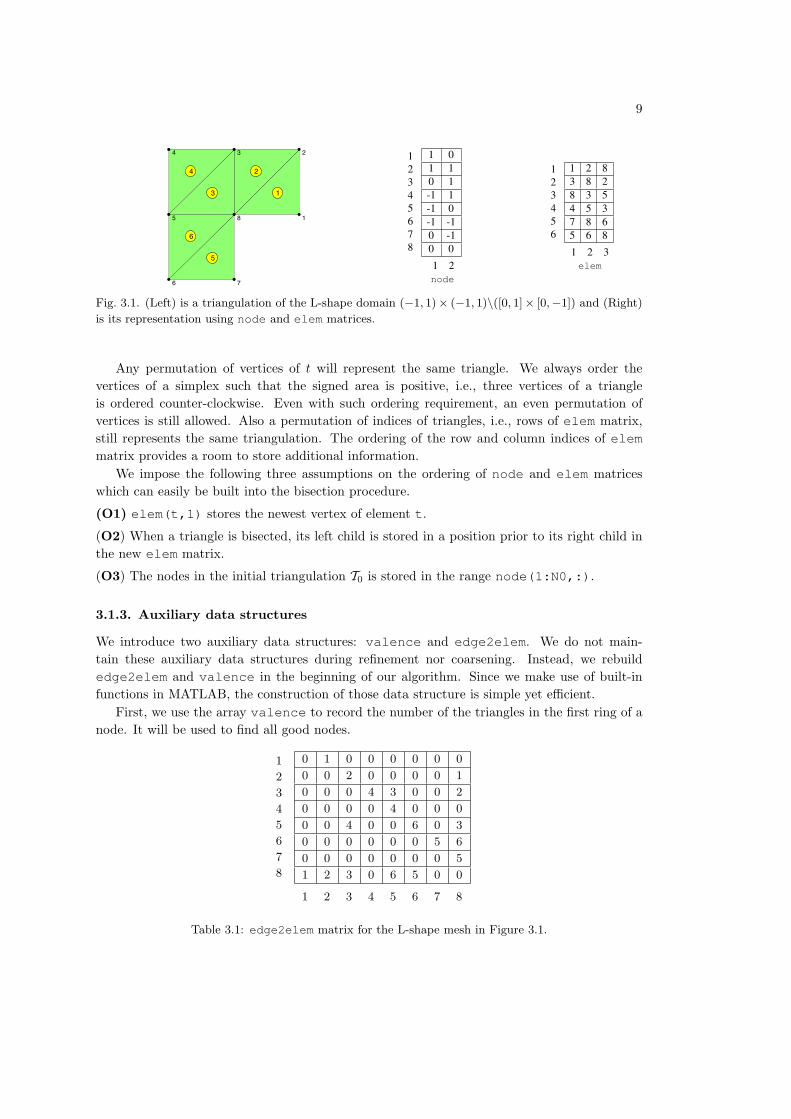
The matrices node(1:N,1:2) and elem(1:NT,1:3) are used to represent a two dimensionaltriangulation, where N is the number of vertices and NT is the number of elements. In thenode matrix node, the first and second rows contain x- and y-coordinates of the nodes inthe mesh. In the element matrix elem, the three rows contain indices to the vertices ofelements. These two matrices represent two different structures of a triangulation: elem forthe topological connectivity of triangles and node for the geometric embedding of vertices. Asan example, node and elem matrices to represent the triangulation of the L-shape domainΩ = (−1, 1)× (−1, 1)\([0, 1]× [0,−1]) are given in the Figure 3.1 (a) and (b).

3.1.2. Assumptions on ordering

An important feature of our implementation is that we only maintain node and elem matrices.At a first glance, one might think it is impossible to coarsen an adaptive mesh without storingthe refinement history. Our trick is: a tree structure of the adaptive procedure can be builtinto the elem matrix by the ordering. We shall make it more precisely in the follows.

Suppose p1, p2, and p3 are three vertices of a triangle t and p4 is the midpoint of therefinement edge E(t). After t is bisected, we name the new element with vertices p1, p2, andp4 the left child and the other the right child. (Left or right is with respect to the directionwalking from p4 to p1.) For example, in Figure 2.1, the left children always appear before theirbrothers (right children) in the elem array.

9

1

234

5

6 7

8

1

2

3

4

5

6

8 LONG CHEN

1

234

5

6 7

8

1

2

3

4

5

6

FIGURE 3. A triangulation of a L-shape domain.

12345678

1 01 10 1-1 1-1 0-1 -10 -10 0

1 2node

123456

1 2 83 8 28 3 54 5 37 8 65 6 8

1 2 3elem

123456789

10111213

1 21 82 32 83 43 53 84 55 65 86 76 87 8

1 2edge

TABLE 1. node,elem and edge matrices for the L-shape domain in Figure 3.

3.3.2. Auxiliary data structure for 2-D triangulation. We shall discuss how to extract the topologicalor combinatorial structure of a triangulation by using elem array only. The combinatorial structure willbenefit the finite element implementation.

edge. We first complete the 2-D simplicial complex by constructing the 1-dimensional simplex. In thematrix edge(1:NE,1:2), the first and second rows contain indices of the starting and ending points.The column is sorted in the way that for the k-th edge, edge(k,1)<edge(k,2). The following codewill generate an edge matrix.

1 totalEdge = sort([elem(:,[1,2]); elem(:,[1,3]); elem(:,[2,3])],2);

2 [i,j,s] = find(sparse(totalEdge(:,2),totalEdge(:,1),1));

3 edge = [j,i]; bdEdge = [j(s==1),i(s==1)];

The first line collect all edges from the set of triangles and sort the column such that totalEdge(k,1)<totalEdge(k,2). The interior edges are repeated twice in totalEdge. We use the summationproperty of sparse command to merge the duplicated indices. The nonzero vector s takes values 1 (forboundary edges) or 2 (for interior edges). We then use find to return the nonzero indices which forms

Fig. 3.1. (Left) is a triangulation of the L-shape domain (−1, 1)× (−1, 1)\([0, 1]× [0,−1]) and (Right)

is its representation using node and elem matrices.

Any permutation of vertices of t will represent the same triangle. We always order thevertices of a simplex such that the signed area is positive, i.e., three vertices of a triangleis ordered counter-clockwise. Even with such ordering requirement, an even permutation ofvertices is still allowed. Also a permutation of indices of triangles, i.e., rows of elem matrix,still represents the same triangulation. The ordering of the row and column indices of elemmatrix provides a room to store additional information.

We impose the following three assumptions on the ordering of node and elem matriceswhich can easily be built into the bisection procedure.

(O1) elem(t,1) stores the newest vertex of element t.

(O2) When a triangle is bisected, its left child is stored in a position prior to its right child inthe new elem matrix.

(O3) The nodes in the initial triangulation T0 is stored in the range node(1:N0,:).

3.1.3. Auxiliary data structures

We introduce two auxiliary data structures: valence and edge2elem. We do not main-tain these auxiliary data structures during refinement nor coarsening. Instead, we rebuildedge2elem and valence in the beginning of our algorithm. Since we make use of built-infunctions in MATLAB, the construction of those data structure is simple yet efficient.

First, we use the array valence to record the number of the triangles in the first ring of anode. It will be used to find all good nodes.

1

2

3

4

5

6

7

8

0 1 0 0 0 0 0 0

0 0 2 0 0 0 0 1

0 0 0 4 3 0 0 2

0 0 0 0 4 0 0 0

0 0 4 0 0 6 0 3

0 0 0 0 0 0 5 6

0 0 0 0 0 0 0 5

1 2 3 0 6 5 0 0

1 2 3 4 5 6 7 8

Table 3.1: edge2elem matrix for the L-shape mesh in Figure 3.1.

10

Second, we use an N × N sparse matrix edge2elem to store the mapping from edges toelement; see Table 3.1. If pipj is an edge of t, then edge2elem(i,j)=t. Due to the orderingof vertices, for an interior edge, edge2elem(j,i) will give another (if it exists) element t′

such that pjpi is an edge of t′. If one of them is zero, it implies that this edge is on the boundary.

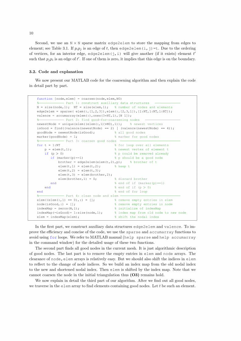
3.2. Code and explanation

We now present our MATLAB code for the coarsening algorithm and then explain the codein detail part by part.

function [node,elem] = coarsen(node,elem,N0)%−−−−−−−−−−−−− Part 1: construct auxiliary data structures −−−−−−−−−−−−−N = size(node,1); NT = size(elem,1); % number of nodes and elementsedge2elem = sparse( elem(:,[1,2,3]),elem(:,[2,3,1]),[1:NT,1:NT,1:NT]);valence = accumarray(elem(:),ones(3*NT,1),[N 1]);%−−−−−−−−−−−−− Part 2: find good−for−coarsening nodes −−−−−−−−−−−−−−−−−−newestNode = unique(elem((elem(:,1)>N0),1)); % newest verticesisGood = find((valence(newestNode) == 2) | (valence(newestNode) == 4));goodNode = newestNode(isGood); % all good nodesmarker(goodNode) = 1; % marker for good nodes%−−−−−−−−−−−−− Part 3: coarsen good nodes −−−−−−−−−−−−−−−−−−−−−−−−−−−−−−−for t = 1:NT % for loop over all elements

p = elem(t,1); % newest vertex of element tif (p > 0) % p could be removed already

if (marker(p)==1) % p should be a good nodebrother = edge2elem(elem(t,2),p); % brother of telem(t,1) = elem(t,2); % keep telem(t,2) = elem(t,3);elem(t,3) = elem(brother,2);elem(brother,1) = 0; % discard brother

end % end of if (marker(p)==1)end % end of if (p > 0)

end % end of for loop%−−−−−−−−−−−−− Part 4: clean node and elem −−−−−−−−−−−−−−−−−−−−−−−−−−−−−−−elem((elem(:,1) == 0),:) = []; % remove empty entries in elemnode(isGood,:) = []; % remove empty entries in nodeindexMap = zeros(N,1); % initialize of indexMapindexMap(¬isGood)= 1:size(node,1); % index map from old node to new nodeelem = indexMap(elem); % shift the nodal index

In the first part, we construct auxiliary data structures edge2elem and valence. To im-prove the efficiency and concise of the code, we use the sparse and accumarray functions toavoid using for loops. We refer to MATLAB manual (help sparse and help accumarray

in the command window) for the detailed usage of these two functions.The second part finds all good nodes in the current mesh. It is just algorithmic description

of good nodes. The last part is to remove the empty entries in elem and node arrays. Theclearance of node,elem arrays is relatively easy. But we should also shift the indices in elem

to reflect to the change of node indices. So we build an index map from the old nodal indexto the new and shortened nodal index. Then elem is shifted by the index map. Note that wecannot coarsen the node in the initial triangulation thus (O3) remains hold.

We now explain in detail the third part of our algorithm. After we find out all good nodes,we traverse in the elem array to find elements containing good nodes. Let t be such an element.

11

We need to find out the brother of t which can be glued with t. By (O2), if we go through allelements from 1 to NT, we always meet a left child before its (right) brother. It is easy to findthe brother of a left child t by brother = edge2elem(elem(t,2),elem(t,1)).

We use T3 in Figure 2.1 as an example to illustrate how our coarsening algorithm works.There is only one good node x in T3; see Figure 3.2. We mark this node and traverse the elementarray elem. In the element array of T3, elements are stored in a possible order indicated by the

an element. We need to find out the brother of t which can be glued with t. By (O2), if we go

through all elements from 1 to NT, we always meet left child first. Thus the following code

will find its brother using the dualEdge array. As we emphasis before, we do not need any

tree structure of the bisection grids.

brother = dualEdge(elem(t,2),elem(t,1));

We now use T3 in Figure 2.1 as an example to illustrate how our coarsening algorithm

works. There is only one good node x in T3; see Figure 3.1(a). We mark this node and

traverse the element array. In the element array of T3, elements are stored in this possible

p T3

t3,1

t3,2 t3,3

t3,4t2,2 t2,3

(a) A compatible bisection triangulation

t3,1 t2,3 t2,2 t3,3 t3,2 t3,4

t2,1 t2,3 t2,2 t3,3 t3,4

t2,1 t2,3 t2,2 t2,4

(b) Coarsening procedure

FIG. 3.1. Good nodes and coarsening procedure.

order indicated by the first row of Figure 3.1(b). We will encounter firstly t3,1 which use x

as its newest vertex. We use the dualEdge to find its brother t3,2 and then glue these two

elements together to get t2,1 back. The place of t3,1 is used to store its father t2,1 and place

of t3,2 is marked to discard by setting its newest vertex as 0; see Figure 3.1(b). After thisstep, x will be left as a hanging node as it is still the newest vertex of t3,3 and t3,4. However

the traverse of element array will continue and encounter t3,3 and glue it with t3,4 and thus

recovery the conformity. Their father t2,4 will be stored in the place of t3,3 which is behind

t2,3. In this way, the ordering of the coarse grid still satisfies the condition (O2). Finally, we

get a mesh T !2 which is different than T2 in Figure 2.1 but still in the class of T(T0). So we

can proceed as before.

This coarsening algorithm can be easily modified for adaptive finite element method

especially for time dependent problems. For example, we could first sort good nodes by some

node-wise local error indicator and then mark part of good nodes for coarsening according

certain marking strategy. For details, we refer to the manual of AFEM@matlab [6]. In this

paper, we shall focus on the application of the proposed coarsening algorithm to iterative

methods for solving algebraic equations.

REFERENCES

[1] I. Babuska and A. K. Aziz. On the angle condition in the finite element method. SIAM Journal on Numerical

Analysis, 13(2):214–226, 1976.

[2] T. C. Biedl, P. Bose, E. D. Demaine, and A. Lubiw. Efficient algorithms for Petersen’s matching theorem. In

Symposium on Discrete Algorithms, pages 130–139, 1999.

[3] P. Binev, W. Dahmen, and R. DeVore. Adaptive finite element methods with convergence rates. Numerische

Mathematik, 97(2):219–268, 2004.

[4] L. Chen. Short implementation of bisection in MATLAB. report, 2006.

[5] L. Chen, M. Holst, and J. Xu. Convergence and optimality of adaptive mixed finite element methods. Sub-

mitted to Mathematics of Computation, 2006.

9

Fig. 3.2. Good nodes and coarsening procedure.

first row in the right of Figure 3.2. We will encounter firstly t3,1 which use p as its newest vertex.We use the edge2elem to find its brother t3,2 and then glue these two elements together toget t2,1 back. The place of t3,1 is used to store its father t2,1 and place of t3,2 is marked to bediscarded by setting its newest vertex as 0; see the second row in Figure 3.2. After this step,p will be left as a hanging node as it is still the newest vertex of t3,3 and t3,4. However thetraverse of element array will continue and encounter t3,3 and glue it with t3,4 and thus recoverythe conformity. Their father t2,4 will be stored in the place of t3,3 which is behind t2,3. In thisway, the ordering of the coarse grid still satisfies the condition (O2). Finally, we get a meshT ′2 which is different than T2 in Figure 2.1 but still in the class of C(T0); so we can proceed asbefore.

4. Application in Multilevel Preconditioning

In this section, we apply the proposed coarsening algorithm to construct multilevel precondi-tioners. We note that most existing multilevel preconditioners on adaptive grids are developedfor the regular refinement [16, 9, 1]. We shall make use of the special structure of bisectiongrids to construct a simple but efficient preconditioner.

4.1. Preliminary

Let Ω be a polygonal bounded domain in R2 and consider the following Dirichlet problem:−div(A(x)∇u) = f in Ω,

u = 0 on ∂Ω,(4.1)

where f ∈ L2(Ω) and A(x) is a uniformly positive definite symmetric matrix function definedin Ω. The weak formulation of (4.1) reads: find u ∈ H1

0 (Ω) such that

(A(x)∇u,∇v) = (f, v) for all v ∈ H10 (Ω), (4.2)

where (·, ·) is the L2 inner product in Ω and H10 (Ω) is the usual Sobolev space of function with

square integrable weak derivatives and vanishing boundary trace in Ω. We approximate (4.2)

12

by the linear finite element discretization. Let T be a conforming and shape-regular grid of thepolygonal domain Ω. We define

V = V(T ) :=v ∈ H1

0 (Ω) : v|t is afine, for all t ∈ T,

and look for a discrete solution uh ∈ V such that

(A(x)∇uh,∇vh) = (f, vh) for all vh ∈ V. (4.3)

Let φiNi=1 be the set of piecewise linear nodal basis functions for interior nodes and uh =∑Ni=1 uiφi. With an abuse of notation, we still denote the vector (u1, u2, . . . , uN )T by u and

(f1, f2, . . . , fN )T by f . Let A = (ai,j)Ni,j=1 ∈ RN×N with aij = (A(x)∇φj ,∇φi) be the stiffnessmatrix. We then end up with the following algebraic system

Au = f. (4.4)

We shall apply the preconditioned conjugate gradient (PCG) method to solve (4.4), namelyuse the conjugate gradient method to solve the preconditioned system BAu = Bf, where B isa symmetric positive definite (SPD) matrix and known as a preconditioner. Note that we donot have to form B explicitly. Instead, given a vector r, we only need the action of B on r, i.e.,the vector Br. A good preconditioner is a balance of the following two considerations:

• the conditioner number κ(BA) is small compared with κ(A);

• the action of B is relatively cheap to compute.

We shall construct multilevel preconditioners using the framework of space decompositionand subspace correction methods [33]. Let V =

∑Lk=0 Vk be a decomposition of V, where

Vk ⊂ V (k = 0, . . . , L) be subspaces of V. Let Ik : Vk 7→ V be the natural inclusion operator(often known as prolongation) and ITk : V 7→ Vk be its adjoint in L2 inner product (oftenknown as restriction.) Let Ak : Vk 7→ Vk be the restriction of A on the subspace Vk. Bychoosing a local subspace solver, often known as a smoother, Rk ≈ A−1

k , we obtain an additivepreconditioner of the form

B =L∑

k=0

ITk RkIk. (4.5)

It is well-known, e.g. [33, 34] that, when Rk is SPD on Vk under L2 inner product, the operatorB defined by (4.5) is also SPD on V under L2 inner product and can be used as a preconditioner.

We now discuss the choice of Rk. Let Dk be the diagonal matrix of Ak. We choose

R0 = A−10 and Rk = D−1

k . (4.6)

Notice that we use a direct solver on the coarsest space V0 since the dimension of V0 is smalland the computational cost is negligible.

With such a choice of smoothers, the preconditioner is uniquely determined by the spacedecomposition. We now present several classical and new preconditioners in Section 4.2.

4.2. Space decomposition and preconditioning

Starting with TL = T ∈ T(T0), we apply our coarsening algorithm iteratively, i.e., Tk−1 =COARSEN(Tk) to obtain a sequence of nested grids. Let Vk = V(Tk) be the linear finite element

13

space on Tk and Nk as the set of interior nodes of Tk for k = 0, 1, . . . , L. When k = L, thesubscript will be skipped. For a given node xk,i ∈ Nk, we use φk,i to denote the canonical nodalbasis function at xk,i in Tk. We shall denote by Vk,i = spanφk,i the one dimensional spacespanned by the nodal basis on Tk.

4.2.1. Hierarchical basis preconditioner

Recall that Gk ⊂ Nk denote sets of good nodes. Let W0 = V0. The so-called hierarchical basis(HB) preconditionerBHB by Yserentant [36, 35] is obtained using the hierarchical decomposition

V =L⊕

k=0

Wk with Wk =⊕

xk,i∈Gk

Vk,i, k = 1, · · · , L. (4.7)

Since our coarsening algorithm will remove all good nodes in the current level, we have

Nk = Nk−1 ∪ Gk. (4.8)

Thus the first decomposition for V in (4.7) is a direct sum. Let pk,i, pk,j ∈ Gk be two differentgood nodes in Tk. Suppose that there exists an element t ∈ Rk,i ∩ Rk,j , then both pk,i andpk,j are the newest vertices of t which is a contradiction. So Rk,i ∩ Rk,j = ∅, and the seconddecomposition in (4.7) for each Wk is also a direct sum. Note that this is the special propertyof nested bisection grids obtained by our coarsening algorithm and may not be true for nestedbisection grids using the tree structure and adaptive grids obtained by the regular refinement.

The hierarchal decomposition (4.7) is of optimal computational complexity and easy toimplement. It is well known [35, 4] that the preconditioner BHB based on (4.7) is almostoptimal in the sense that

κ(BHBA) ≤ CL| log hmin|, (4.9)

where hmin = mint∈T diam(t).

4.2.2. BPX preconditioner

To stabilize the HB preconditioner, Bramble, Pasciak and Xu [10] propose to use the so-calledBPX preconditioner BBPX based on the space decomposition

V =L∑

k=0

Vk with Vk =∑

xk,i∈Nk

Vk,i, k = 1, . . . , L. (4.10)

It is well known [16, 33, 29] that there exists a constant C independent of the problem size suchthat

κ(BBPXA) ≤ C. (4.11)

The decomposition (4.10), however, has lots of overlapping. For adaptive grids, it is possiblethat Vk results from Vk−1 by just adding a handful of basis functions (maybe even only one.)Thus smoothing on both Vk and Vk−1 leads to a lot of redundancy. In the worst scenario, thecomplexity of smoothing could be as bad as O(N2) [26].

14

4.2.3. Three-point hierarchical basis preconditioner

We note that the difference between (4.7) and (4.5) is that the nodes set for finite elementspaces in the k-th level. One natural idea is to choose nodal sets Sk such that

Gk ⊂ Sk ⊂ Nk, k = 1, . . . , L. (4.12)

On the one hand, Sk is chosen more than Gk to stabilize the decomposition. On the other hand,Sk should have the same order of cardinality as Gk to preserve optimal complexity.

Let pi ∈ Gk be the midpoint of Ei. Let pi,1 = pi and pi,2, pi,3 be the two end nodes of Ei(or the so-called parents of pi). We define Sk := pi,1, pi,2, pi,3 | pi ∈ Gk, W0 = V0, and thedecomposition

V =L∑

k=0

Wk with Wk =∑

p∈Sk

Vp, k = 1, · · · , L, (4.13)

where Vp = spanφp is the space spanned by the nodal basis functions on Tk.We call the corresponding multilevel preconditioner Three-point Hierarchical Basis (THB)

preconditioner and denoted by BTHB. It is obvious that #Sk = 3#Gk and thus the computa-tional complexity of BTHB is at most three times of BHB. In [14], it is proved that

κ(BTHBA) ≤ C. (4.14)

We conclude that (4.13) is a stable decomposition with optimal complexity.

4.2.4. Locally orthogonal hierarchical basis preconditioner

We propose another improvement over the HB decomposition (4.7) by enhancing the coarsespace. For convenience of presentation, we now give a local index of the vertices in ωpi

; seeFigure 4.1 for a pictorial description.

DHBpreconditioner. We give a space decompositionswhich is a good balance of (4.10)

and (4.5). Motivated by the modified HB preconditioner given by Qin and Xu [37], we simply

add the high frequency in the finest space into the decomposition. Namely we can use the

following decomposition

V =L!

k=0

Wk +"

i!NVL,i. (4.14)

For#

VL,i, we use D"1 as the smoother. In this case, the preconditioner for this decom-

position is like a combination of HB and diagonal preconditioners. We thus call it DHB and

denoted by BDHB . Theoretically it will not remove the log N factor in (4.13). But numeri-

cally BDHB is comparable to BPX preconditionerBBPX .

THB preconditioner. We note that the difference of (4.10) and (4.5) is the the nodes set

for finite element spaces in k-th level. One natural idea is to choose sets Sk such that

Gk ! Sk ! Nk, k = 1, . . . , L. (4.15)

On one hand, Sk is chosen to stabilize the decomposition. On the other hand, Sk should have

the same order of cardinality as Gk to preserve optimal complexity.

Let xi " Gk be the midpoint ofEi. For convenience of presentation, we now give a local

index of the vertices of !xi; see Figure 4.1 for a pictorial description. Let xi,1 = xi and

xi,2, xi,3 be the two end nodes of Ei (or the so-called immediate neighbors of xi). Motivated

by the stable three-point wavelet constructed by Stevenson [32], we shall define

Sk := xi,1, xi,2, xi,3|xi " Gk,

and the decomposition

V =L"

k=0

$Wk with $W0 = V0, $Wk ="

x!Sk

Vx, k = 1, · · · , L, (4.16)

where Vx = span"x is the space spanned by the nodal basis functions on Tk.

12

4

3

5

2 3

4

1

FIG. 4.1. Local index. Left: node 1 is an interior node; right: node 1 is on the physical boundary of domain!.

We shall call the correspondingmultilevel preconditionerTHB (Three-point Hierarchical

Basis) preconditioner and denoted by BTHB . It is obvious that #Sk = 3#Gk and thus the

computational complexity of BTHB is at most three times of BHB . In [15], it is shown that

(4.16) is a stable decomposition in both two and three dimensions. We conclude that (4.16)

is a stable decomposition with optimal complexity.

13

Fig. 4.1. Local indices of nodes for a compatible bisection.

Consider the local patch ωpiand the piecewise linear function space

Vk,i := Vk(ωpi) = spanφi,j | j = 1, . . . , Ji,

where Ji = 5 if pi is an interior point and Ji = 3 if pi is on the boundary. We define

ψi,j := φi,j + αi,jφi,j ∈ Vk(ωpi) and αi,j = − (φi,j , φi,1)A(φi,1, φi,1)A

,

such that (ψi,j , φi,1)A = 0. We construct a local A-orthogonal decomposition

Vk,i = span(φxi)⊕Qk−1,i, (4.15)

15

where Qk−1,i := ψi,2, ψi,3, . . . , ψi,5 ⊂ Vk(ωpi). We name this preconditioner correspond-

ing to (4.15) as Locally Orthogonal Hierarchical Basis (LOHB) preconditioner. This simplemodification gives a much better hierarchical basis preconditioner.

In fact, we should point out the equivalence of LOHB preconditioner and hierarchical basismultigrid (HBMG) [4], where the special hierarchical structure of bisection grids using ourcoarsening algorithm plays an important role. Thus we can estimate the condition numberof κ(BLOHBA) using the results by Bank, Dupont and Yserentant [4]. More precisely, in oursetting, suppose A(x) is piecewise constant on the coarse mesh T0, then

κ(BLOHBA) ≤ CL| log hmin|, (4.16)

and the constant C is independent of the jump of diffusion coefficients and the size of the linearsystem. Although (4.16) still depends on the mesh size, the computational results show thatthe LOHB preconditioner outperforms the other preconditioners.

Remark 4.1 (Implementation of Prolongation and Restriction) The local prolongationoperator, J kk−1 : Qk−1,i → Vk,i is given by

(J kk−1u)(pi,1) =

Ji∑

j=2

αi,ju(pi,j) pi,1 ∈ Gk

u(pi,1) pi,1 ∈ Nk\Gk.The restriction operator will be the transpose of the prolongation operator. Algorithmically, itis a simple modification of HB preconditioner.

We present the following algorithm for the LOHB preconditioner BLOHB. We shall use eand r to indicate that we are solving the residual equation Ae = r in each subspace. Thealgorithm will compute Br for any given vector r.

Algorithm e = LOHB(r)rL = r

for k = L : 1rk−1 = (J kk−1)trk % restriction

end

e0 = A−10 r0 % exact solver

for k = 1 : Lek = Rkrk % local smootherek = ek + J kk−1ek−1 % prolongation

end

e = eLEND Algorithm

4.3. Numerical examples

We use the residual-type error estimator introduced by Babuska and Miller [2] for generalsecond-order elliptic equations. The bulk marking strategy by Dorfler [17] with θ = 0.3 is usedin our simulation for marking. For comparison, we always start the preconditioned conjugategradient (PCG) methods from the zero initial guess and the stopping criteria is the relativeresidual error is less than tol = 10−6. All numerical experiments are performed with MATLAB7.0 on a PC with Intel Pentium IV 1.0GHz and 1GB RAM.

16

Example 1: Poisson equation on L-shaped domain

In this example, we consider the second-order elliptic equation (4.1) with A ∈ R2×2 beingthe identity matrix and f = 0 on a L-shaped domain Ω := (−1, 1)2\[0, 1) × (−1, 0] with areentrant corner. We choose the Dirichlet boundary condition g such that the exact solution tobe u(r, θ) = r

23 sin( 2

3θ) in polar coordinates. It is well-known that the solution u ∈ Hs(Ω) fors < 5

3 has a corner singularity at the origin.We start the adaptive finite element method from a compatibly labeled initial grid T0 (Figure

4.2(a)). An example adaptive grid is given in Figure 4.2(b). Since there is a point-singularity,

(a) Initial grid: isosceles triangles. (b) Adaptive grid obtained by newest vertex bisections.

Fig. 4.2. Initial and refined meshes used in Example 1.

the adaptive refinement are done very locally (see Figure 4.2(b)). It is interesting to find out howmany good-for-coarsening nodes we actually have on each level for highly graded adaptive gridsgenerated by the AFEM loop (1.1). The results are reported in Table 4.1, from which we can seethat degree of freedom (DOF) on each level (generated by our coarsening algorithm) decreasesgeometrically as for the uniform refinement case. Since the decay rates α = DOFk−1/DOFkare almost constant for any two consecutive levels, we only show the rates for the last two levelsin the table.

Table 4.1 suggests that we only need to call the coarsening algorithm iteratively a few timesto obtain a coarse enough grid. For example, for this problem, after 5 steps of coarsening, thedegree of freedom left is only about 3% of the original number of unknowns.

DOF 9628 13339 18648 26097 36528

level: J 4586 6365 8934 12532 17793

level: J − 1 2402 3393 4699 6572 9164

level: J − 2 1276 1749 2425 3448 4733

level: J − 3 684 943 1293 1765 2425

level: J − 4 375 486 696 945 1293

Decay rate 0.548 0.515 0.538 0.535 0.533

Table 4.1: Number of good nodes on each level in five different adaptive grids for Example 1.

We present number of iterations for PCG with CPU time in the bracket using differentpreconditioners in Table 4.2. From this table, we have a couple of observations: (1) Theiteration number of HB preconditioner increases slightly as DOF increases because the decom-position (4.7) is not stable. (2) The BPX preconditioner is uniform, but it could take moreCPU time than the HB preconditioner. The advantage of the former is more significant forlarge problems. (3) The THB is a good balance of HB and BPX. (4) The LOHB is the bestamong the four in terms of CPU time and iteration steps.

17

DOF 9628 13339 18648 26097 36528

HB 31 (0.37) 31 (0.48) 31 (0.67) 36 (0.98) 36 (1.42)

BPX 23 (0.48) 23 (0.71) 22 (0.92) 25 (1.48) 25 (2.32)

THB 18 (0.35) 19 (0.50) 18 (0.71) 20 (0.87) 20 (1.40)

LOHB 10 (0.21) 10 (0.29) 10 (0.37) 11 (0.54) 11 (0.79)

Table 4.2: Number of iterations (CPU time in seconds) by PCG (initial guess u0 = 0 and tol = 10−6)

with different preconditioners for Example 1.

.

Example 2: Discontinuous coefficient problem

In this example, we employ a test example designed by Kellogg [20] with discontinuousdiffusion coefficient. Consider the partial differential equation (4.1) with Ω = (−1, 1)2 and thecoefficient matrix A is piecewise constant: in the first and third quadrants, A = a1I; in thesecond and fourth quadrants, A = a2I. For f = 0, the exact solution in polar coordinates hasbeen chosen to be u(r, θ) = rγµ(θ), where

µ(θ) =

8>>><>>>:cos`(π

2− σ)γ

´cos`(θ − π

2+ ρ)γ

´if 0 ≤ θ ≤ π

2,

cos (ργ) cos ((θ − π + σ)γ) if π2≤ θ ≤ π,

cos (σγ) cos ((θ − π − ρ)γ) if π ≤ θ ≤ 3π2,

cos`(π

2− ρ)γ

´cos`(θ − 3π

2− σ)γ

´if 3π

2≤ θ ≤ 2π,

and the constants

γ = 0.1, ρ = π/4, σ = −14.9225565104455152, a1 = 161.4476387975881, a2 = 1.

We see that the solution u produces a very strong singularity at the origin (barely in H1(Ω)).See Figure 4.3 for an example of adaptive grids and its associated finite element solution.

Fig. 4.3. Finite element solution uh (left) on the adaptive grid with DOF = 164 (right).

The point singularity in the example is much stronger than the one in the previous testexample. The adaptive grids are extensively concentrated at the origin. Due to this effect, thenumber of marked elements are quite small each iteration. The number of good nodes on first 5levels are shown in Table 4.3. The decay rate of the number of DOF is slight worse than beforebut still close to a constant. The number of iterations required for each method are listed inTable 4.4. We observe similar behaviors as in Example 1. Especially the LOHB is the bestamong the four in terms of CPU time and iteration steps.

From the experiments above, we have already seen that the LOHB preconditioner performsthe best. Now we want to check how sensitive it is to the magnitude of the jump in the coefficientmatrix A. We use the same domain with f = 1 and g = 0. We keep a1 = 1 and change a2 from

18

DOF 7095 9708 13726 19821 28956

level: J 2351 3280 4792 7068 10569

level: J − 1 1780 2364 3245 4624 6648

level: J − 2 1067 1443 2029 2884 4147

level: J − 3 662 873 1234 1765 2554

level: J − 4 393 552 788 1132 1666

Decay rate 0.593 0.632 0.638 0.641 0.652

Table 4.3: Number of good nodes on each level in five adaptive grids for Example 2.

DOF 7095 9708 13726 19821 28956

HB 26 (0.26) 25 (0.40) 27 (0.62) 27 (1.0) 33 (1.51)

BPX 24 (0.48) 24 (0.60) 24 (0.85) 24 (1.48) 27 (1.93)

THB 19 (0.29) 19 (0.42) 19 (0.56) 19 (0.89) 21 (1.26)

LOHB 10 (0.17) 10 (0.23) 10 (0.32) 10 (0.59) 10 (0.68)

Table 4.4: Number of iterations (CPU time in seconds) by PCG (initial guess u0 = 0 and tol = 10−6)

with different preconditioners for Example 2.

1 to 104 on the same grid (uniform refinement by newest vertex bisections.) From Table 4.5,we can see that the preconditioner BLOHB is robust with respect to the size of jumps.

DOF 961 1985 3969 8065 16129

a2 = 1 10 8 9 11 9

a2 = 10 10 9 10 11 10

a2 = 102 10 9 10 11 10

a2 = 103 10 9 10 11 10

a2 = 104 10 9 10 11 10

Table 4.5: Number of iterations by PCG (initial guess u0 = 0 and tol = 10−6) with the LOHB

preconditioner for Example 2.

5. Application in Time Adaptive Mesh Refinement

When solving time dependent problems with local features, it is usually difficult if evenpossible to design optimal meshes a priori. Hence, adaptive mesh refinement and adaptive timestepping are important to achieve optimal complexity. In order to obtain nearly optimal meshesfor time dependent problems, the COARSEN step in (1.1) is crucial as local features oftenmove in time. Standard coarsening algorithms (see [31] for details) requires data structuresto store a refinement tree in order to keep shape regularity after coarsening. As we have seenbefore, the proposed new coarsening algorithm, on the contrary, does not need refinement treeinformation.

We take an example from Chen and Jia [15] to test the performance of the proposed coars-ening algorithm when applied to adaptive mesh refinement. Consider the heat equation in twospatial dimensions for u(x, s):

du

ds−∆u = f x ∈ Ω, s ∈ (0, T ], (5.1)

19

where Ω := (−1, 1) × (−1, 1) and T = 1. We choose the right hand side function f(x, s) suchthat the exact solution

u(x, s) = β(s) exp(−25|x− α(s)|2)

withα(s) = s− 0.5, β(s) = 0.1

(1− exp(−104α(s)2)

).

A posteriori error estimations and adaptive algorithms for linear parabolic problems havebeen discussed by many researchers [6, 7, 18, 19, 30, 28, 23, 15, 22]. Traditionally we write aposterior error estimators in element-wise which is more convenient for marking elements withlarge local error for refinement. We could also easily rewrite error estimators side-wise or node-wise. There are also error estimators which are intrinsically node-wise; see [27] for example. Agenuine a posterior error estimators for parabolic problems can be written as follows

∫ T

0

|||u− Uh|||2Ω ds ≤ Cη2

init +N∑

n=1

kn

((ηnspace)2 + (ηntime)2 + (ηncoarse)2

),

where, as their names suggest, ηinit is an initial error estimator, ηnspace is a spatial error estimator,ηntime is a time error estimator, and ηncoarse measures error introduced by coarsening; see [31] fordetails.

We now briefly discuss the node-wise time-space adaptive mesh refinement scheme for timedependent problems. Note that we assume that the newest vertex bisection as our refinementalgorithm.

Algorithm 5.1 (Adaptive Algorithm for Evolution Problems) Start with initial timestep size k0, initial mesh T0, and initial solution U0

h . Set n = 1 and sn = k0.(i) Compute initial error indicator ηinit.

If ηinit is too large, refine the patch Rpif ηinit(p) is large; goto (i).

While sn ≤ T , do (a)–(e):(a) Solve for Unh and compute time error indicator ηntime.If ηntime is too large, reduce time step kn, update sn, and goto (a).(b) For every p ∈ N (Tn), compute spatial and coarsening error indicators:

if ηnspace(p) is too large, refine Rp;if ηnspace(p) + ηncoarse(p) is too small, coarsen Rp (if p is a good node).

(c) If the mesh was changed in (b):solve for Unh and compute error indicators again;if ηntime is too large, goto (a);if ηnspace is too large, goto (b);

otherwise, accept the current solution Unh .(d) If ηntime is small, enlarge kn+1.(e) Let sn+1 = sn + kn+1 and n = n+ 1.

Remark 5.1 (An example of error indicators for the heat equation) For completeness,we now give node-wise error indicators adapted from [27] for the heat equation (5.1):

ηinit(p) = ‖U0h − u(0)‖ωp

ηnspace(p) = ‖h 12 Jnh ‖γp + ‖h(fn − fnp )‖ωp

ηn−1coarse(p) = ‖∇(Un−1

h − InUn−1h )‖ωp

ηntime = ‖∇(Unh − InUn−1h )‖Ω,

20

where the superscript n refers to the time level. In : V(T n−1)→ V(T n) is the standard transferoperator from , h is the local mesh size, γp is the set all interior edges of ωp, Jnh is the jump ofgradient of Unh over interior edges, and fnp is the average of fn on the local patch ωp.

Now we show the performance of our coarsening algorithm. We report energy error atdifferent time in Figure 5.1 together with number of degrees of freedom (DOF) and time stepsize. From Figure 5.1, we find the adaptive refined mesh and time step are adapted to the exactvery well. In particular, when the solution becomes very smooth in space but changes very fastin time around time level 0.5, the time stepsize becomes small and spatial mesh size becomeslarge. We also show two sample meshes in Figures 5.2 and 5.3.

Fig. 5.1. History of energy error, spatial DOF and time stepsize. Left: energy error; middle: spatial

degree of freedom; right: time stepsize.

Fig. 5.2. Solution and automatically generated mesh at the initial time (t = 0.0).

Acknowledgments. The first author was supported in part by NSF Grant DMS-0811272,and in part by NIH Grant P50GM76516 and R01GM75309. The second author was supportedby NSF Grant DMS-0915153.

References

[1] B. Aksoylu, S. Bond, and M. Holst. An adyssey into local refinement and multilevel precondi-

tioning III: Implementation and numerical experiments. SIAM Journal of Scientific Computing,

21

Fig. 5.3. Solution and automatically generated mesh at the final time (t = 1.0).

25(2):478–498, 2003.

[2] I. Babuska and A. Miller. The post-processing approach in the finite element method. Part 3:

A posteriori error estimates and adaptive mesh selection. International Journal for Numerical

Methods in Engineering, 20:2311–2324, 1984.

[3] W. Bangerth, R. Hartmann, and G. Kanschat. deal.ii — a general purpose object oriented finite

element library. ACM Transactions on Mathematical Software, 33(4):24, Aug. 2007. Article 24,

27 pages.

[4] R. E. Bank, T. Dupont, and H. Yserentant. The hierarchical basis multigrid method. Numerische

Mathematik, 52:427–458, 1988.

[5] T. C. Biedl, P. Bose, E. D. Demaine, and A. Lubiw. Efficient algorithms for Petersen’s matching

theorem. J. Algorithms, 38(1):110–134, 2001.

[6] M. Bieterman and I. Babuska. The finite element method for parabolic equations. I. A posteriori

error estimation. Numer. Math., 40(3):339–371, 1982.

[7] M. Bieterman and I. Babuska. The finite element method for parabolic equations. II. A posteriori

error estimation and adaptive approach. Numer. Math., 40(3):373–406, 1982.

[8] P. Binev, W. Dahmen, and R. DeVore. Adaptive finite element methods with convergence rates.

Numerische Mathematik, 97(2):219–268, 2004.

[9] F. A. Bornemann and H. Yserentant. A basic norm equivalence for the theory of multilevel

methods. Numerische Mathematik, 64:455–476, 1993.

[10] J. H. Bramble, J. E. Pasciak, and J. Xu. Parallel multilevel preconditioners. Mathematics of

Computation, 55(191):1–22, 1990.

[11] J. M. Cascon, C. Kreuzer, R. H. Nochetto, and K. G. Siebert. Quasi-optimal convergence rate for

an adaptive finite element method. SIAM Journal on Numerical Analysis, 46(5):2524–2550, 2008.

[12] L. Chen. Short implementation of bisection in MATLAB. In P. Jorgensen, X. Shen, C.-W.

Shu, and N. Yan, editors, Recent Advances in Computational Sciences – Selected Papers from the

International Workship on Computational Sciences and Its Education, pages 318 – 332. World

Scientific Pub Co Inc, 2007.

[13] L. Chen. iFEM: an innovative finite element methods package in MATLAB. Submitted, 2009.

[14] L. Chen, R. H. Nochetto, and J. Xu. Local multilevel methods on graded bisection grids. In

Preparation, 2009.

[15] Z. Chen and F. Jia. An adaptive finite element algorithm with reliable and efficient error control

for linear parabolic problems. Math. Comp., 73:1167–1194, 2004.

[16] W. Dahmen and A. Kunoth. Multilevel preconditioning. Numerische Mathematik, 63:315–344,

1992.

22

[17] W. Dorfler. A convergent adaptive algorithm for Poisson’s equation. SIAM Journal on Numerical

Analysis, 33:1106–1124, 1996.

[18] K. Erickson and C. Johnson. Adaptive finite element methods for parabolic problems. i. a linear

model problem. SIAM Journal on Numerical Analysis, 28(1):43–77, 1991.

[19] K. Eriksson and C. Johnson. Adaptive finite element methods for parabolic problems II: Optimal

error estimates in l∞l2 and l∞l∞. SIAM Journal on Numerical Analysis, 32(3):706–740, 1995.

[20] R. B. Kellogg. On the Poisson equation with intersecting interface. Appl. Aanal., 4:101–129, 1975.

[21] I. Kossaczky. A recursive approach to local mesh refinement in two and three dimensions. Journal

of Computational and Applied Mathematics, 55:275–288, 1994.

[22] O. Lakkis and C. Makridakis. Elliptic reconstruction and a posteriori error estimates for fully

discrete linear parabolic problems. Math. Comp., 75(256):1627–1658 (electronic), 2006.

[23] C. Makridakis and R. H. Nochetto. Elliptic reconstruction and a posteriori error estimates for

parabolic problems. SIAM J. Numer. Anal., 41(4):1585–1594, 2003.

[24] W. F. Mitchell. Unified Multilevel Adaptive Finite Element Methods for Elliptic Problems. PhD

thesis, University of Illinois at Urbana-Champaign, 1988.

[25] W. F. Mitchell. A comparison of adaptive refinement techniques for elliptic problems. ACM

Transactions on Mathematical Software (TOMS) archive, 15(4):326 – 347, 1989.

[26] W. F. Mitchell. Optimal multilevel iterative methods for adaptive grids. SIAM Journal on

Scientific and Statistical Computing, 13:146–167, 1992.

[27] K.-S. Moon, R. H. Nochetto, T. von Petersdorff, and C.-S. Zhang. A posteriori error analysis

for parabolic variational inequalities. Mathematical Modelling and Numerical Analysis (M2AN),

41(3):485–511, 2007.

[28] R. H. Nochetto, A. Schmidt, and C. Verdi. A posteriori error estimation and adaptivity for

degenerate parabolic problems. Mathematics of Computation, 229(220):1–24, 1999.

[29] P. Oswald. Multilevel Finite Element Approximation, Theory and Applications. Teubner Skripten

zur Numerik. Teubner Verlag, Stuttgart, 1994.

[30] M. Picasso. Adaptive finite elements for a linear parabolic problem. Comput. Methods Appl. Mech.

Engrg., 167(3-4):223–237, 1998.

[31] A. Schmidt and K. G. Siebert. Design of adaptive finite element software, volume 42 of Lecture

Notes in Computational Science and Engineering. Springer-Verlag, Berlin, 2005. The finite element

toolbox ALBERTA, With 1 CD-ROM (Unix/Linux).

[32] E. G. Sewell. Automatic generation of triangulations for piecewise polynomial approximation. In

Ph. D. dissertation. Purdue Univ., West Lafayette, Ind., 1972.

[33] J. Xu. Iterative methods by space decomposition and subspace correction. SIAM Review, 34:581–

613, 1992.

[34] J. Xu and L. Zikatanov. The method of alternating projections and the method of subspace

corrections in Hilbert space. Journal of The American Mathematical Society, 15:573–597, 2002.

[35] H. Yserentant. On the multi–level splitting of finite element spaces. Numerische Mathematik,

49:379–412, 1986.

[36] H. Yserentant. Two preconditioners based on the multi-level splitting of finite element spaces.

Numerische Mathematik, 58:163–184, 1990.