1

A Cognitive Fault Diagnosis Systemfor Distributed Sensor NetworksCesare Alippi, IEEE Fellow, Stavros Ntalampiras, and Manuel Roveri

Abstract—The paper introduces a novel cognitive Fault Di-agnosis System (FDS) for distributed sensor networks whichtakes advantage of spatial and temporal relationships amongsensors. The proposed FDS relies on a suitable functional graphrepresentation of the network and a two-layer hierarchicalarchitecture designed to promptly detect and isolate faults. Thelower processing layer exploits a novel Change Detection Test(CDT) based on Hidden Markov Models (HMMs) configured todetect variations in the relationships between couples of sensors.HMMs work in the parameter space of linear time invariant(LTI) dynamic systems approximating, over time, the relationshipbetween two sensors; changes in the approximating model aredetected by inspecting the HMM likelihood. Information pro-vided by the CDT layer is then passed to the cognitive onewhich, by exploiting the graph representation of the network,aggregates information to discriminate among faults, changes inthe environment and false positives induced by the model biasof the HMMs.

Index Terms—Fault diagnosis; distributed sensor network;intelligent sensors; hidden Markov model.

I. INTRODUCTION

SENSOR networks monitoring a real environment are proneto faults or aging phenomena, whose impact affects the

overall system performance. In fact, permanent or transientfaults can influence the sensors, the analog electronics, thedigital part of the embedded system inducing, in the best case,functional errors in the processing chain. In turn, erroneousinformation generates a strong side effect on the subsequentcontrol chain leading to wrong decisions and inappropriatecontrol actions.A Fault Diagnosis System plays the important role of su-

pervising the process operations in order to detect, isolate andidentify a potential fault and, possibly, design accommodationactions [1]. The main components of the FDS are learned fromthe available data when physical descriptions for the processare unavailable. Not rarely, an appropriate model describingthe underlying process is built and its validity assessed overtime by the FDS through a change inspection mechanism,e.g., by observing changes in some features such as theapproximating model residuals or parameters.Unfortunately, when a change in the model is detected by

the FDS, three situations might arise:• “model bias”: The model is no more representing thecurrent data due to model approximating inefficiencies;

C. Alippi, S. Ntalampiras and M. Roveri are with the Dipartimento di Elet-tronica e Informazione, Politecnico di Milano, Milan, Italy, 20133 IT e-mail:{alippi,ntalampiras,roveri}@elet.polimi.it (see http://sagroup.ws.dei.polimi.it)

• “change in the environment”: the environment is time-variant and the trained model is no more able to explainthe current data;

• “fault”: a sensor or a component of a unit is affected bya fault which induces an error in the datastream.

Distinguishing among the above perturbation classes is amajor achievement which, whenever possible, allows the FDSfor isolating the fault/change and proposing the appropriateaccommodation action.Published FDSs for sensor networks generally do not allow

for distinguishing between faults and changes in the environ-ment [2]. Moreover, the model bias is generally considerednegligible, a hardly satisfied hypothesis in many applications.A review of the literature is given in Section II.The paper presents a novel cognitive FDS acting on sensor

datastreams that removes the strong hypotheses assumed in theliterature; as such, under reasonable assumptions, it deals withthe model bias case and proposes a method for discriminatingbetween faults and changes in the environment.Hidden a-priori information related to spatial and temporal

relationships among sensor datastreams (both explicit andimplicit) is exploited, leading to a functional dependency graphwhere nodes are the sensors and arcs are associated with thesensor-to-sensor relationship. In particular, for each sensorcouple, a HMM is designed, which receives the parametersof a LTI model approximating the relationship. As such,spatial redundancy is modelled with a HMM operating in theparameter space of LTI dynamic models embedding the timedependency. When the likelihood between the HMM-basedlearning machine and the new incoming datastream falls belowa threshold (which can be learnt as well) a change is detected(HMM-based Change-Detection Test) at the detection layer.The cognitive layer of the FDS, activated in response to achange alarm raised by the detection one, separates faults fromtime variant and bias cases by operating on the dependencygraph of the network. At the same time, it allows us forisolating the fault for a possible subsequent accommodationphase.The novelties of the proposed approach can be summarised

as follows:• introduction of a dependency graph representing thetemporal and spatial relationships among the sensor units;

• suggestion of the joint use of LTI models and HMMs fordesigning a Change-Detection Test;

• design of a cognitive graph-based approach able to dis-tinguish among changes induced by model bias, sensorfaults or changes in the environment.

2

The paper is organized as follows. Section II surveys thefault diagnosis literature for sensor networks. Section IIIpresents the modelling methodology for functional relation-ships in sensor networks, while Section IV introduces theproposed hierarchical cognitive FDS. Experimental results aregiven in Section V and conclusions drawn in the last Section.

II. RELATED LITERATURE

The fault diagnosis system literature for sensor networks(also called sensor validation) embraces two main approachesexploiting information either coming from a single sensoror a set of sensors (a detailed review of the fault-detectionliterature can be found in [1], [2]). The former approach aimsat detecting faults by inspecting data coming from a singlesensor. Here, we have the limit checking method [3], whichraises an alarm when the physical quantity under monitoringovercomes a threshold, and change-detection methods e.g., [4],[5], which aim at detecting variations in the statical behaviourof the physical phenomenon under observation. Techniquesfollowing the latter approach, and based on physical or ana-lytical redundancy methods, detect faults by exploiting redun-dant/correlated information coming from multiple sensors.Physical redundancy requires redundant sensors measuring

the same physical quantity, possibly at different resolutionlevels. For instance, [6] suggests a fuzzy-based technique tocorrect data subject to sensor drifts and intermittent faults inthe case of truly redundant sensors. Differently, analytical re-dundancy exploits functional relationships among the sensorswhich measure different, but correlated, physical quantities.Most design approaches for fault diagnosis rely on this conceptand assume that a mathematical model of the healthy systemis available. Fault diagnosis is achieved by comparing actualobservations with those coming from the prediction modeland, then, inspecting residual values or differences amongredundant sensors [6]. [7] suggests a fuzzy rule approach forvalidation of highly correlated sensors (or quasi-redundantsensors). Several techniques based on artificial neural net-works have been presented in the literature (e.g., [8]–[10]).For example, [8] suggested the use of autoassociative neuralnetworks and Kohonen maps for sensor failure detection inredundant/correlated sensors. [9] describes the use of neuralnetworks in sensor fault detection with specific attentionto flight control systems. [10] applies a feedforward neuralnetwork to data coming from a space shuttle main engine.Other analytical redundancy-based approaches consider, forexample, the use of Principal Component Analysis [11] andthe Nadaraya-Watson statistical estimator [12]. Although thesemethods may achieve satisfactory performance levels theyassume availability of an accurate model.Fault detection and diagnosis issues have also been widely

addressed within the Computational Intelligence community.For example, [13] suggests a model-based process supervisionfor fault detection and identification where a nonlinear ob-server based on a Radial basis function (RBF) neural networkis used to approximate the unknown nonlinear dynamics (thelinear part is assumed to be known). In the case of faults, adifferent RBF is used to identify the nonlinear characteristics

of the fault profile. Similarly, [14] presents a robust faultdiagnosis framework for detecting and approximating stateand output faults affecting nonlinear multi input-multi outputdynamical systems. Here, the nonlinear component of theprocess and sensor uncertainties are assumed to be unknownbut bounded. [15] suggests a FDS for distributed systemsbased on a set of finite state machines (e.g., the model de-scribing the message exchange within a transmission protocol).The nominal and the faulty behaviour of the system areassumed to be known; the detection phase relies on an observercomparing the ideal with the measured output datastreams.Several fault detection and diagnosis systems for application-specific scenarios can also be found in [16]–[20].A practical way to conduct group level analysis for fault

diagnosis is the K over N approach [21]: a change is detectedwhen K out of N functionally related sensors detect it. Eventhough the approach may provide reasonable performance, itsuffers from a severe disadvantage: it treats all sensors iden-tically. Moreover, detection performance is heavily influencedby K . Lower values of K lead to low detection latency at theexpenses of higher false positive rates. The opposite holds.Echo state network (ESN) solutions have been recently

considered for fault diagnosis, mainly at the sensor level. Forinstance, [22] exploits ESNs to detect faults in the temperatureand moisture sensors of a mote-class device. The ESNs aretrained by using data coming from the nominal state andno spatial redundancy among different units is taken intoaccount. [23] suggests an ESN for identifying anomalies inthe concentration of natural gas in underground coal mines.The ESN is trained on normal (safe condition) data comingfrom CH4, CO2, CO, O2 and pressure sensors; the detectionmechanism is based on the difference between the output ofthe ESN and that of the sensor (with a threshold definedaccording to the Neyman-Pearson test).A different approach was suggested in [24], [25] and

[26] where hidden semi-Markov models (HSMM) have beenproposed to improve fault detection and identification. Inparticular, [24] suggested the use of HSMMs trained ontemperature, speed and direction of the wind as well as thehistorical values of the PM2.5 concentration to predict futureinstances. [25] and [26] exploit HSMMs for health monitoringof hydraulic pumps. Wavelet-based features of the vibrationalsignals coming from the pumps have been used to train thefault detection/identification system and a fault dictionary isrequested to detect/isolate the erroneous conditions. All aboveapproaches work at the single sensor level by exploitingtemporal relationships and do not consider existing spatialdependencies among the sensor units (which is one of thenovelties of the proposed approach).It should be noted that methods present in the literature

neither consider a dynamic predictive model coupled witha HMM nor exploit the functional graph of the network tocarry out a cognitive analysis able to separate faults fromapproximating model bias and environmental changes as wedo here.

3

III. MODELING FUNCTIONAL RELATIONSHIPSIN SENSOR NETWORKS

Let us consider a sensor network composed of N fixedsensing units deployed within the environment P . Each unitcan host up to M sensors opening views on different physicalaspects of P (e.g., temperature, humidity, change in slope,vibrations, rain intensity). Each j-th sensor of the i-th unitacquires a scalar datastream Xi,j .We neither require a specific topology for the network nor

a particular communication routing protocol. The FDS can bein execution at the remote control room (where all data arereceived) or at the base stations (e.g., within a hierarchicaltopology setup) if the network can be partitioned into func-tionally disjoint sub-networks (each of which containing abase station). Data communication among units must hencebe intended between the units and the base station/controlroom where the FDS algorithm is executed. A synchronizationalgorithm (e.g., [27]) should be considered to guarantee timeconsistency among samples whenever poor clock generators(as those in sensor networks) are available (the clock skewcan easily rise to seconds in few days [28]).

A. Modeling the network: the dependency graph

The cognitive framework for fault diagnosis relies on theability to model functional relationships among the acquiredviews of P . In more detail, each relationship captures spatialand temporal dependency from data provided by a genericcouple of sensors. Fig. 1 shows an example of a sensor networkwith functional dependencies.A direct relationship exists between a couple of sensors

of the same type (e.g., temperature vs temperature): if datas-treams Xi,j and Xv,j , i != v are correlated, an arc linking thej-th sensor of unit i with its counterpart of unit v is introduced.For instance, two clinometers insisting on the same connectedstructure are related; those deployed far apart probably are not.An indirect relationship can be introduced between two

generic sensors by means of a third entity. For instance, aclinometer and a strain gauge sensor whose readouts are af-fected by a parasitic thermal effect will be indirectly correlatedthanks to the temperature dependency. Such a relationship canexist between sensors mounted in the same unit (i.e., X i,j andXi,u, j != u) or present in different units (i.e., X i,j and Xv,u,i != v, j != u). Of course, indirect relations are mitigatedby the presence of compensation mechanisms; in this caseinformation useful for the analysis must be extracted beforecompensation takes place.De facto, direct and indirect relationships introduce a

functional constraint between couples of sensors. Denote byf{(i,j),(u,v)} the functional relationship between the generic j-th sensor of unit i and the v-th sensor of unit u. The nodes ofG are the network sensors; the arcs represent the functionalrelationships between couples of sensors. Given a network, notall the (N "M)(N "M # 1) relationships in G are relevant.For example, two sensors might be weakly correlated due totopological or phenomenological reasons or not correlated atall in one direction due to causality.

sensor 1

sensor 2

sensor 3

Unit 1

Unit 2

Unit 3

Unit 4

sensor 1

sensor 2

sensor 3

sensor 1

sensor 2

sensor 3

sensor 1

sensor 2

sensor 3

direct

indirect

Fig. 1. Direct and indirect relationships in a distributed monitoring network.

X11

X12

X13

X21

X22

X23

X31

X32

X33

Sub-graph 1Sub-graph 2

Sub-graph 3

X41

X42

X43

Sub-graph 4

Fig. 2. The dependency graph of the sensor network og Fig. 1.

The reduced dependency graph is then derived from G anddefined as graph

GR = {V,E}

where V is the set of nodes of the graph representing theN " M sensors and E a set collecting all arcs associatedwith functional relationships whose correlation is above athreshold. The level of dependency associated with relation-ship f{(i,j),(u,v)} is here chosen to be the linear correlationindex between two datastreams Xi,j and Xv,u: when the peakof the crosscorrelation is above !min, !min being a suitablytuned threshold, the relationship is considered to be relevantand worth to be included in E; other dependency indexes canbe surely derived and considered. Let F be the set of functionalrelationships with correlation index larger than !min.We remove from GR isolated nodes.Fig. 2 shows the graph-based representation of the sensor

network of Fig. 1: we have 4 units; each unit is a subgraph

4

representing the mounted sensor.

B. Modeling the relationship between two sensors with aHidden Markov ModelIn the following we assume that the relationship between

a couple of sensors f{(i,j)(u,v)} can be modelled either as atime-invariant (TI) dynamic system or as a finite sequenceof TI dynamic systems satisfying the HMM hypotheses. Noassumption about the linearity of the relationship is made.Let’s imagine to model now a f{(i,j)(u,v)} with the Single-

Input Single-Output (SISO) Linear (LTI) model of form

A(z)Xi,j(t) =B(z)

F (z)Xv,u(t) +

C(z)

D(z)d(t) (1)

where z is the backward time-shift operator, d(t) an inde-pendent and identically distributed (i.i.d.) random variableaccounting for the noise, A(z), B(z), C(z), D(z), and F (z)represent the z-transform functions of model parameters "A,"B , "C , "D and "F , respectively. In the following we assumeA(z), B(z), C(z), D(z), and F (z) to be either time-invariantor time-varying but following a Markov chain model.A given SISO model M (e.g., ARX, ARMAX or OE) is

then an element locally approximating f !{(i,j),(u,v)}, y! =

M("), " $ DM parametrized in " = ["A, "B, "C , "D, "F ].The use of linear models allows us to apply theoretical

results delineated in [29], [30]. More specifically, considera training dataset composed of NT {input,output} couples{u(t), y(t)}NT

t=1, a loss function VNT = 1NT

!NT

(y # y!)2

whose minimization provides an estimate ", of the optimalparameter "! = argmin!"DM limNT#+$ E [VNT ].Under the assumption that each f{(i,j),(u,v)} function sat-

isfies the exponential stability for closed loop (i.e., accurateapproximations of Xi,j(t) can be generated given finite timewindows of Xi,j(.) and Xv,u(.)), from [30] we have that

"NTP

% 12 (" # "!) % N (0, I) when NT & '; (2)

P $ Rp&p is the covariance matrix of the p parameters of themodel.It comes out that, under the above assumption and a

sufficiently large N the distribution underlying the parametervectors " is a multivariate Gaussian, with mean "! and covari-ance matrix P . We emphasize that the same framework canbe applied to Extreme-Learning Machines [31] or ReservoirComputing Networks [32].By following the (2) a HMM with parameters " ruled

by a mixture of gaussians becomes a natural solution toapproximate f{(i,j),(u,v)}. The nodes of the HMM represent,de facto, a probabilistic ensemble of LTI models somehowminimizing the model bias ||y! # f{(i,j),(u,v)}|| if the trainingset is sufficiently informative. More in detail, the HMM isdefined as

H = {n,F , A,#}, (3)

where n is the number of states, F = {p1, . . . , pn} is the setof probability density functions (pdfs) associated with eachstate, A is the n" n state transition probability matrix and #the n"1 initial state distribution vector. Thanks to (2) the pdf

associated with each state can be safely modelled as a mixtureof Gaussians (GMMs). In fact, the GMM of the i-th state isdefined as

pi("|!i) =Ki#

k=1

wk,iN ("|µk,i,"k,i) (4)

where Ki is the number of Gaussian mixtures for the i-thstate, wk,i is the weight for state i and Gaussian mixturek, !i = [µ1,i, . . . , µki,i,"1,i, . . . ,"ki,i] with µk,i and "k,i

the mean vector and the covariance matrix for state i andGaussian mixture k, respectively. We considered a mixture ofGaussian functions with diagonal covariance matrices since,an L-th order full covariance GMM can be achieved using adiagonal covariance GMM of a larger order [33]. Thus, themixture of Gaussian solution is as effective as the former ata much lower computational cost. We remark that we shouldconsider a single Gaussian function with full covariance matrixto model a state of the process.By modelling parameters " with a HMM we mitigate the

effect of model bias and time variance provided that thetraining set is sufficiently informative and explores both timevariance and nonlinearity.

IV. THE COGNITIVE FAULT DIAGNOSIS SYSTEMThe proposed FDS is organized as the two-layer architecture

of Figure 3. The lower level is composed by a set of ChangeDetection Tests (CDTs) each of which monitoring the sta-tionarity of a relationship associated with a couple of sensorsin GR. Each HMM CDT works in the parameter space " todetect variations in the relationship between the two sensors(the CDT is described in the Section IV-A). Unfortunately,a CDT is not able to distinguish among changes induced bya fault in a sensor, an environmental change in P or a falsepositive generated by a model bias since such classes are indis-tinguishable. To address this issue the upper level of the FDShas been designed to be able to discriminate between faults,changes in P and false positives by exploiting informationassociated with the network graph GR. The upper level of theFDS relies on a cognitive algorithm aggregating decisions andlog-likelihood information provided by the HMM-CDT in thelower level. The cognitive aggregation level is described inSection IV-B.

X(i1,j1) X(v1,u1)

detection likelihood

X(i|E|,j|E|)X(v|E|,u|E|)

detection likelihood

Cognitive Aggregation Level

Detection Fault/Change in the environment

Fault diagnosis system

HMM-based CDT on |E|

HMM-based CDT on 1

Fig. 3. The proposed FDS.

5

1- Let {X(i,j)(t), 1 ( t ( T0} and {X(v,u)(t), 1 ( t ( T0}be the training set of sequences X(i,j) and X(v,u);

2- Create T0 #NT + 1 overlapping windows of NT data;3- Estimate parameters " for each data window andgenerate the sequence ST = {"1, . . . , "T0%NT+1};

4- Train H = {s,F , A,#} on ST ;5- Th = min1's'T0%NT+1 l{(i,j),(u,v)}(s) as in Eq. (5);6- t = T0, s = T0 #NT + 1;repeat

7- t = t + 1;8- Acquire X(i,j)(t) and X(v,u)(t);9- s = s + 1;10- Estimate the parameter "s on

{X(i,j)(t), t#NT + 1 ( t ( t} and{X(v,u)(t), t#NT + 1 ( t ( t};

11- Compute l{(i,j),(u,v)}(s) as in Eq. (5);12- if l{(i,j),(u,v)}(s) < Th then13- Raise an alarm: change detected;

enduntil (1);Algorithm 1: The HMM-CDT for a generic functionalrelationship f{(i,j),(u,v)} in GR.

A. The HMM-based Change Detection TestThe proposed HMM-CDT aims at evaluating, by means of

a HMM, the evolution over time of the parameters "s approx-imating the relationship f{(i,j),(u,v)}; X(i,j) is the output andX(v,u) the input of the LTI. " are estimated on overlappingwindows of NT data.The HMM-CDT requires the training of HMMH{(i,j)(v,u)},

devoted to model the relationship between sensors (i, j) and(u, v) H{(i,j),(u,v)}, is trained by means of the Baum-Welchalgorithm [34].During the operational life, the parameter "s is estimated

on the s-th window of data and the log-likelihood

l{(i,j),(u,v)}(s) = P ("1, . . . , "s|H{(i,j),(u,v)}) (5)

computed and indicating how likely the sequence of estimatedparameters "1, . . . , "s has been generated by the H{(i,j),(u,v)}.The log-likelihood is computed with the Viterbi algorithm[35].When the log-likelihood decreases below a threshold Th, a

change in the relationship is detected (the sequence of inputsis no more recognized by the learning machine). Threshold T h

can be defined by the operator, who exploits a-priori availableinformation. However, if not available, Th can be estimatedas the minimum value assumed by the log-likelihood in thetraining (or better validation) sequence. Th can be scaledby a coefficient factor c1 (with 0 ( c1 ( 1) to tradeoffthe robustness of the machine w.r.t. false positives and falsenegatives.The HMM-based CDT is detailed in Algorithm 1.

B. The cognitive aggregation levelThe cognitive level aggregates the information coming from

all sensor units to distinguish among faults, changes in P

1- HMM-CDT associated with H{(i,j),(u,v)} detected achange in the s-th data window;

2- Partition the graph into sets E+, E% and EP accordingto Eq. (7), (8), (9) ;

3- Compute S+, S%, SP according to Eq. (10), (11) and(12);

4- Compute T+, T%, TP according to Eq. (13), (14) and(15);

5- if SP < TP then6- Change in P detected;else

7- if S+ < T+ and S% < T% then8- Model Bias in H{(i,j),(u,v)} detected;

else9- if S+ < T+ then10- Fault at sensor X(i,j) detected;

else11- Fault at sensor X(v,u) detected;

endend

endAlgorithm 2: The algorithm which combines the HMM-based CDTs for change identification and isolation.

and false positives induced by model bias in the HMMCDT. Differently from the HMM-CDTs that are executedsequentially, the cognitive aggregation level is activated only inresponse to a detection alarm raised by at least a CDT-HMM.Detections and log-likelihoods of others CDTs are used toassess and, possibly, identify the change.The motivating idea is that a change in P for a given type of

sensors must be perceived also by a set of other CDTs, at leastas a decrement in the log-likelihood values (not necessarilybelow the threshold). Differently, in the case of faults, only theCDTs associated with relationships that have either as inputor output the faulty sensor are affected by the change. Finally,if a false positive occurs, other CDTs should not be affected.To evaluate the reliability of the information coming from

HMM-CDTs we introduce a reliability index w{(i,j),(u,v)} forthe HMM H{(i,j),(u,v)} defined as

w{(i,j),(u,v)} =#

1's'T0%NT+1

l{(i,j),(u,v)}(s). (6)

Weights are computed on the training set; the weighted re-duced graph is the reduced graph augmented with the weightinformation.Definition: Let E+ be the set of functional relationships

such that either the source or the target node of the arc isX(i,j), i.e.,

E+ = {f(i,j)(v,u) $ {F # f(i,j)(v,u)}|(i = i and j = j) or (v = i and u = j)}. (7)

Definition: Let E% be the set of functional relationshipssuch that either the source or the target node of the arc is

6

X11

X12

X13

X21

X22

X23

X31

X32

X33

X41

X42

X43

w(1,1)(2,1)

w(3,3)(1,3)

w(1,2)(2,3)

w(1,3)(1,2)

w(3,3)(3,1)

w(4,1)(2,3)

w(3,2)(4,2)

w(3,1)(2,2)

(a)

w(4,3)(4,2)

X11

X12

X13

X21

X22

X23

X31

X32X33

X41

X42

X43

(b)

w(1,1)(2,1)

w(1,2)(2,3)

w(3,3)(1,3)

w(3,2)(4,2)

w(3,1)(2,2)

w(4,1)(2,3)

w(1,3)(1,2)

w(4,3)(4,2)

w(3,3)(3,1)

Fig. 4. The cognitive aggregation level: a) the reduced weighted dependency graph; b) an example of arcs partitioning into E+, E! and EP given a changedetected in the functional relationship f{(3,3),(1,3)} .

X(v,u), i.e.,

E% = {f(i,j)(v,u) $ {F # f(i,j)(v,u)}|(i = v and j = u) or (v = v and u = u)}. (8)

Definition: Let EP be the set of functional relationshipswhose source or target node is neither X(iq,jq) nor X(vq,uq),i.e.,

EP = F # {E+ ) E% ) {f{(i,j)(v,u)}} (9)

After a change detected in f{(i,j)(v,u)} the remaining F # 1functional relationships of the weighted reduced dependencygraph are partitioned into sets E+, E% and EP . The reasonfor the partitioning is as follows:

• a fault in sensor X(i,j) affects the functional relationshipsin E+ but not those in E% and EP ;

• a fault in the sensor X(v,u) affects the functional rela-tionships in E% but not those in E+ and EP ;

• a change in P affects the functional relationships in E%,E+ and EP ;

• a model bias affecting H{(i,j),(u,v)} would mostly affectthe functional relationship between (i, j) and (u, v) but,in principle, not the functional relationships in E%, E+

and EP provided that approximating relationships arecharacterised by different bias contributions.

An example of partitioning is shown in Figure 4a; in Figure4b a change is detected in relationship f{(3,3)(1,3)}. We have

E+ = {f{(3,3)(3,1)}};E% = {f{(1,3)(1,2)}};EP = {f{(1,1)(2,1)}, f{(1,2)(2,3)}, f{(3,1)(2,2)}, f{(4,1)(2,3)},

f{(3,2)(4,2)}, f{(4,3)(4,2)}}.

Defined s to be the index of the data window where theHMM CDT detected a change, the proposed aggregation level

computes the normalized sum of the log-likelihoods, suitablyweighted according to (6), of the arcs in E+, E% and EP :

S+ =1!

E+ w{(i,j),(u,v)}

#

E+

w{(i,j),(u,v)}l{(i,j),(u,v)}(s); (10)

S% =1!

E! w{(i,j),(u,v)}

#

E!

w{(i,j),(u,v)}l{(i,j),(u,v)}(s); (11)

SP =1!

EP w{(i,j),(u,v)}

#

EP

w{(i,j),(u,v)}l{(i,j),(u,v)}(s). (12)

The core of the cognitive aggregation level is thus the abilityto compute S+, S% and SP by exploiting information comingfrom all the relationships of the weighted reduced dependencygraph. S+, S% and SP measure how the change detected inthe relationship f{(i,j)(v,u)} is perceived in other relationships.If a fault affects sensor (i, j), S+ should decrease, while S%

and SP should not. Similarly, if a fault affects sensor (u, v),S% should decrease, S+ and SP not. If a change in P occurs,SP should decrease as well as S+ and S%.To detect decreases in S+, S% and SP we rely on a simple

thresholding mechanism. The thresholds for S+, S% and SP

are computed as follows:

T+ =1!

E+ w{(i,j),(u,v)}

#

E+

w{(i,j),(u,v)}Th,{(i,j),(u,v)}; (13)

T% =1!

E! w{(i,j),(u,v)}

#

E!

w{(i,j),(u,v)}Th,{(i,j),(u,v)}; (14)

TP =1!

EP w{(i,j),(u,v)}

#

EP

w{(i,j),(u,v)}Th,{(i,j),(u,v)}. (15)

where Th,{(i,j),(u,v)} is the minimum value assumed by thelog-likelihood in the training sequence for the HMM-CDTof functional relationship f{(i,j),(u,v)} as described in theprevious section. Thresholds T P , T+ and T% can be scaled

7

by a coefficient factor c2 with 0 ( c2 ( 1 to increase therobustness w.r.t. false positives. We suggest to select c2 > c1since we want to detect decreases in the likelihood which didnot yet raised an alarm (and hence the likelihoods are abovetheir respective thresholds). In fact, if we consider c2 ( c1,we would require that the weighted average of the likelihoodscomputed in Eq. (10,11,12) decreases below the weightedaverage of the thresholds for change detection Ths computedin Eq. (13,14,15) but this is a nonsense since relationships inE+, E% and EP did not detect a change yet.To sum up, the cognitive aggregation level acts as follows:• If SP decreases below threshold T P , a change in P isidentified;

• If SP > TP and S+ < T+ (or S% < T%), a fault insensor X(i,j) (or in sensor X(v,u)) is detected;

• If SP > TP and S+ > T+ and S% > T%, a falsepositive induced by a model bias is detected.

If both S+ and S% are above their respective thresholds,we can raise the alarm fault in either X(i,j) or X(v,u) but wecannot isolate the affected sensor since not enough informationis available. Further analyses could thus be performed at thesub-graph level by considering the relationships associatedwith the sub-graph (or the sub-graphs) of the sensors affectedby the change. The cognitive aggregation level algorithm isgiven in Algorithm 2.

Comments on real sensor networksThe effectiveness of the proposed cognitive fault diagnosis

system relies on the ability to exchange data among the unitsof the distributed sensor network. This can be achieved witha single, multi-hop or hybrid communication depending onthe nature of the deployment and the chosen technology. Ingeneral, a centralized solution is taken, i.e., the FDS algorithmis executed at the remote control room where all data aresent and energy availability is not an issue. Differently, ifthe reduced dependency graph can be partitioned into notoverlapping sub-networks then the FDS can be distributedat the sub-network level and executed at the base station(where local data instances are conveyed before activatingthe remote communication). A further particular case is thatof isolated units. Here, only indirect functional relationshipscan be created (unless sensor redundancy is envisaged) andthe FDS can be executed directly at the unit level (if enoughenergy and computational power is available).Not rarely, sensor units working in a real scenario are

characterized by the missing data issue, whose severity de-pends on two distinct causes. Data missing can either beinduced by permanent/transient faults affecting the units orelectromagnetic disturbances preventing the data packet tobe delivered to the target (packet loss) within a best effortcommunication protocol framework. When the missing of datais associated with the communication aspect (e.g., noisy chan-nel), a reliable communication protocol could be consideredto compensate the problem at the expenses of an increasedenergy consumption and communication complexity overhead:this solution might not be acceptable in limited resource-basedembedded systems.

The effect of transient faults either affecting the commu-nication channel or the functionality of the units can bepartly – and often effectively – mitigated by resorting todata reconstruction algorithms. This aspect must be takeninto account whenever the datastream is expected to sufferfrom the missing data problem. In this case, reconstructiontechniques for distributed sensor networks, e.g., see [36], [37],and [38], reconstruct the missing data by exploiting temporaland spatial redundancies among sensors. Clearly, the operationintroduces an additional uncertainty on the missing data unlessthe reconstruction mechanism is optimal. That said, the faultdiagnosis system presented here works in the parameter spacewith parameters learned on a window of data. It is expectedthat the impact on the parameter is negligible if the number ofmissing data is much smaller than the size of the data window;the opposite holds. However, we know exactly when the dataare missing, situation that, as per se, constitutes a fault. This apriori information might suggest us to postpone the diagnosisphase until a good window of data is available (at the expensesof a delay in the detection of a potential change) or assign aconfidence to the outcome of the FDS also function of thenumber of missing data.

V. EXPERIMENTS AND RESULTS

The aim of the experimental section is to show both thedetection and the recognition ability of the proposed FDS.To achieve this goal we considered two different scenarios:detection and recognition. The first refers to the case wherea change affecting a datastream must be detected as soon aspossible while maintaining under control false positives andfalse negatives. The latter refers to the case where a sensorfault or a change in P affects a sensor network and theproposed FDS has to promptly detect and recognize it.To evaluate the effectiveness of the proposed FDS we

considered both synthetic data and real measurements comingfrom various sources. Section V-A presents the detectionexperiments, while the recognition experiments are shown inSection V-B.The HMMs of the proposed CDT have been configured in a

fully connected topology (ergodic HMMs). The torch machinelearning framework [39] was used both to construct andestimate the accuracy of the HMMs. The maximum number ofk-means iterations for cluster initialization was set to 50; theBaum-Welch algorithm used to estimate the transition matrixwas bounded to 25 iterations with a threshold of 0.001 betweensubsequent iterations. The number of explored states rangesfrom 3 to 7 while the number of Gaussian components usedto build the GMM belongs to the {1, 2, 4, 8, 16, 32, 64, 128,256, 512} set.The main parameters of the cognitive FDS are detailed in

Table I; their values have been experimentally determined.The SISO model (1) considered for the HMM-based CDTs

is an ARX model whose autoregressive and exogenous com-ponent orders range from 1 to 6. The right order for time lagsand parameters are learned during the training phase.In the detection scenario, the proposed FDS is compared

with the parity equation approach [1], [5], which inspects

8

Symbol Value Description!min 0.5 Threshold on cross-correlationc1 0.1 Correction factor for Thc2 0.5 Correction factor for T+, T! and TP

TABLE ITHE PARAMETERS OF THE PROPOSED FDS.

the discrepancy between the process behavior and the pro-cess model describing the nominal change-free behavior. Thethreshold is set as the highest discrepancy on unseen trainingdata. When the discrepancy overcomes this threshold, a changeis detected.Differently, in the recognition scenario, we compared the

proposed FDS with the K/N fusion method [21], commonlyused to combine decisions made by different sensors. Anenvironmental change is detected when at least K sensors(over the total number of N sensors) detect a change. Assuggested in [21], K is fixed at N/2.Five figures of merit have been defined to evaluate the

detection and the recognition accuracy:• False positive index (FP): it counts the times a test detectsa change in the sequence when there it is not (percentage).

• False negative index (FN): it counts the times a changeis not detected when there it is (percentage).

• Detection Delay (DD): it measures the time delay indetecting a change (number of samples).

• Change-in-the-environment recognition rate (CE): it mea-sures the times a change in the environment is correctlyidentified (percentage).

• Fault recognition rates (F): it measures the times a faultis correctly identified (percentage).

• Isolation rates: it measures the times a fault is correctlyisolated, i.e., the sensor affected by the fault is correctlyidentified (percentage).

A. DetectionThis scenario, which examines the ability of the proposed

FDS to detect statistical changes in datastreams, encompassesa synthetic dataset, a dataset coming from the Barcelona waternetwork simulator and a dataset coming from a monitoringsystem working under real-world conditions for rock collapseforecasting.1) Synthetic Dataset: This experiment refers to data gen-

erated by ARX(2,2) model

Xi(t) = a1Xi(t# 1) + a2Xi(t# 2)+

b1Xj(t# 1) + b2Xj(t# 2) + e(t)

where a1 = 0.5, a2 = 0.2, b1 = 0.1, b2 = 0.3, and e(t) %N(0,$2) is a zero-mean Gaussian noise parameterized in itsvariance $2. The exogenous input Xj has been modeled as

Xj(k) = 5 sin(0.05k) + 3 sin(0.09k) + %(k),

where %(k) % N(0, 0.012) is a zero-mean Gaussian noiseaffecting the exogenous input.Each experiment lasts 12000 samples with the first 4000

samples used for training. After 4000 samples an artificially

injected perturbation & affects the coefficients of the ARXmodel. We considered two types of perturbations, i.e., abruptchanges and drifts, reflecting the occurrence of a permanentor transient fault or a smooth aging effect in the sensors,respectively. In case of abrupt changes, the parameters of theARX model suddenly change from " = {a1, a2, b1, b2} to"" = {a1(1 + &), a2(1 + &), b1(1 + &), b2(1 + &)}. In caseof drift changes, the parameters of the ARX model slowlychange from " to "", which is now reached at the end ofthe experiments. The values of lambda considered in theexperiments are & = {0.03, 0.05, 0.07, 1}.To evaluate the performance of the proposed method

we considered different strengths for the noise $ ={0.01, 0.02, 0.04, 0.07, 0.1}. Simulation results are averagedover 250 runs.The results of synthetic data for the abrupt perturbation case

are shown in Table II. We see that the FP rate and the delayare increasing with the noise level. As expected, the FN ratereduces as & increases. Similarly, for a given noise level $,the mean delay reduces as & increases. We observe that evenin highly noisy conditions, the proposed solution guaranteeshigh detection accuracy and low detection delays. The parityequation approach provides lower performances both in termsof detection accuracy and delay. In particular, the proposedmethod always guarantees lower mean delays, much lowerFN rates (at the expenses of a slightly higher FP rates at low$s). The results of the drift type of change presented in TableIII are in line with those of the abrupt change ones.2) Barcelona water network simulator: This dataset con-

sists in simulated data of the water distribution network ofthe city of Barcelona [40]. While the real network is quitecomplex (200 district metering areas and 400 control points),the network simulator provides flow meter data with respect totwo related in time pumps for a time period of approximatelyone month. Eight types of faults are artificially induced inthe second pump. The ability of the FDS to detect faults istested by conducting an experiment for each type of fault. Eachexperiment lasts 1488 samples: the first 744 samples representthe normal situation, while in the remaining 744 samples thesecond pump is affected by a fault. Figure 5 shows the 8datasets for the second pump.The proposed FDS is trained with 500 data samples to

model the nominal state and 100 to determine the threshold.We report that all eight faults were correctly identified as

faults by the proposed FDS with no occurrences of falsepositives or false negatives. The types of faults along withthe respective detection delays are given in Table IV. Thewindow of the CDT has length NT = 40 samples. Theproposed FDS detects each category of faults with a relativelysmall latency. Differently, the parity equation method provideshigher detection delays and fails to detect two types of faults(negative offset abrupt additive and negative offset incipientadditive).3) Rock collapse forecasting system: This experiment refers

to a real-world dataset provided by a real-time monitoringsystem for rock fall forecasting [41] designed by our groupand deployed in the Alps.Here we consider measurements coming from a novel

9

Proposed approach Parity equation method

" of the noise # FP (%) FN (%) Delay FP (%) FN (%) Delay(# of samples) (# of samples)

0.010.03 2.50 4.77 8 0 33.84 61.120.05 2.50 0 8 0 31.12 60.670.07 2.50 0 8 0 31.12 600.1 2.50 0 8 0 28.09 59.04

0.020.03 2.78 8.59 8 0 53.46 630.05 2.78 0 8 0 51.93 61.630.07 2.78 0 8 0 51.27 61.280.1 2.78 0 8 0 50.85 61.45

0.040.03 8.52 7.48 9.8 2.56 53.53 59.130.05 8.52 0 9 2.56 51.91 57.630.07 8.52 0 8.7 2.56 51.28 61.480.1 8.52 0 8.6 2.56 50.86 61.52

0.07

0.03 9.82 8.46 12 13.43 54.32 48.830.05 9.82 0 10.9 13.43 51.92 52.950.07 9.82 0 9.7 13.43 51.29 52.680.1 9.82 0 9 13.43 50.83 51.75

0.10.03 12.28 6.86 16 26.46 54.97 36.030.05 12.28 0 15.7 26.46 52.07 43.930.07 12.28 0 15.1 26.46 51.27 35.130.1 12.28 0 15 26.46 50.84 31.45

TABLE IIApplication D1 - Abrupt case - DETECTION RESULTS OF THE PARITY EQUATION APPROACH AND THE PROPOSED CHANGE DETECTION METHODS.

Proposed approach Parity equation method

" of the noise Lambda FP (%) FN (%) Delay FP (%) FN (%) Delay(# of samples) (# of samples)

0.01 0.1 1.02 0 12 0.72 36.74 48.30.02 0.1 2.19 0.2 12 2.59 41.8 49.30.04 0.1 7.92 1.69 14 4.19 44.75 510.07 0.1 10.1 4.4 18.1 13.47 48.73 53.60.1 0.1 12.34 5.75 21.46 24.45 49.5 55.8

TABLE IIIApplication D1 - Drift case - DETECTION RESULTS OF THE PARITY EQUATION APPROACH AND THE PROPOSED CHANGE DETECTION METHODS.

Fault type Proposed FDS Parity equationDD (Samples) DD (Samples)

Freezing abrupt additive 12 42Freezing incipient 12 44

Negative offset abrupt additive 34 -Negative offset incipient additive 56 -Positive drift abrupt additive 10 21Positive drift incipient additive 12 20

Noise abrupt additive 11 275Noise incipient additive 12 280

TABLE IVTHE DETECTION DELAYS FOR EACH FAULT TYPE IN THE BARCELONA

WATER DISTRIBUTION NETWORK TESTBED.

generation of intelligent clinometer sensors (see Fig. 6) whichhave an internal thermal sensor to correct and compensateon-line the measurements. The goal is to exploit the indirectrelationship between the clinometer and temperature sensorsto detect faults or changes in P .In particular, we considered the temperature and clinometer

measurements recorded from August 1st 2011 until October31th 2011. The sampling rate of each sensor is one sampleper hour. The dataset is composed of 2100 samples, the first500 samples composing the training sequence, the next 100samples used to compute the threshold and the remaining sam-ples constitute the test set. We considered an ARX(1,2) model

Temperature sensor

Clinometer sensor

Fig. 6. An example of a intelligent clinometer sensor working in the rockcollapse forecasting system deployed in the Alps.

family as it provides the best reconstruction performance. Thewindow of the CDT has length NT = 100 samples.Figure 7 presents data and results of both the proposed

HMM-based CDT and the parity equation approach. In par-ticular, the upper two subfigures show the temperature andthe clinometer measurements while the bottom two show thedetections using the HMM-based CDT and residual thresh-olding method. We observe that the flat part of the signal atabout sample 1300 (due to a communication fault) is correctlydetected. Interestingly, the detection around sample 1500 can

10

200 400 600 800 1000 1200 1400

2468

10x 103 Freezing abrupt additive

200 400 600 800 1000 1200 1400

2468

10x 103 Freezing incipient

200 400 600 800 1000 1200 14000

0.005

0.01Negative offset abrupt additive

200 400 600 800 1000 1200 14000

0.005

0.01Negative offset incipient additive

200 400 600 800 1000 1200 1400

2468

10x 103 Positive drift abrupt additive

200 400 600 800 1000 1200 1400

2468

10x 103 Positive drift incipient additive

200 400 600 800 1000 1200 14000

0.005

0.01Noise abrupt additive

Samples200 400 600 800 1000 1200 1400

0

0.005

0.01Noise incipient additive

Samples

Fig. 5. The 8 datasets of the faulty pump of the Barcelona Water Network simulator. The red dotted lines represent the time instances that the fault affectsthe pump and the green dashed one represents the time instance a fault is detected by the proposed FDS.

be associated to a transient false detection induced by modelbias, while the detections at the end of the experiment can beassociated with a change in P . These considerations will beconfirmed by the results presented in the recognition scenarioin which both the communication fault and the change in theenvironment will be perceived by the cognitive level. On thecontrary the residual based method produces a false positivealarm at value 500 and it detects the environmental changes atthe end of the sequence but it fails to detect the communicationerror.

B. RecognitionWe consider a synthetic dataset, and datasets coming from

a rock collapse forecasting system and the Great Barrier ReefOcean Observing System.1) Synthetic datasets: The synthetic experiment refers to a

network composed of N = 20 units. Datastreams of the firstten units are modelled as

Xj(t) = u1 sin(u2t) + u3 sin(u4t) + %(t),

where 1 ( j ( 10, u1, u2, u3 and u4 are randomly selectedin the [4.5, 5.5], [0.04, 0.06], [2.5, 3.5], [0.08, 0.1] intervals,respectively, and %(t) % N(0, 0.012) is a zero-mean Gaussiannoise.The remaining 10 units provide data according to models

X10+j(t) = a1X10+j(t# 1) + a2X10+j(t# 2)+

b1Xj(t# 1) + b2Xj(t# 2) + e(t)

where a1, a2, b1, b2 are randomly selected in intervals[0.45, 0.55], [0.15, 0.25], [0.05, 0.15], [0.25, 0.35], respectivelyand e(t) % N(0,$2) is a zero-mean Gaussian noise ofvariance $2. Thus, to generate data we impose 10 relationshipswhere units Xj , 1 ( j ( 10 represent the inputs, while unitsXj , 11 ( j ( 20 represent the outputs. The data generationgraph is depicted in Fig. 8, while the reduced dependencygraph GR is fully connected and is omitted for brevity.Each experiment lasts 16000 samples with the first 4000

samples used for training the HMMs. The following 4000samples are used by each relationship to learn its ownthreshold (Th). At sample 12000 a perturbation & affectingthe coefficients of the ARX model is artificially injected.Experiments are averaged over 200 runs.When an environmental change is considered, the perturba-

tion & affects all relationships of the data generation graph.We consider both abrupt and drift perturbations to modelsudden or slowly drifting changes, respectively. In case ofabrupt changes, the parameters of the ARX model move from" = {a1, a2, b1, b2} to "" = {a1(1 + &), a2(1 + &), b1(1 +&), b2(1 + &)}. In case of a drift, the parameters of theARX model change slowly from " to "", which is reachedat the end of the experiment. The values of lambda are& = {0.01, 0.05, 1}.On the contrary, when a fault is considered, only one

sensor is affected by the change under the single fault caseassumption. The fault is inject in an a-priori selected sensor(i.e., sensor #20) and its values were artificially increased as

11

Proposed approach K/N equation method# of the noise " FP (%) FN (%) DD CE FP (%) FN (%) DD CE

(Samples) (%) (Samples) (%)

Abrupt

30.01 1.7 1.7 29 94 2.1 10.8 31.92 250.05 1.7 1.6 27.9 94 2.1 11 29.2 280.1 1.7 1.5 25.9 95 2.1 11.3 26.6 30

40.01 2.6 0.7 29.4 95 2.7 16.3 42.9 310.05 2.6 0.6 27.4 97 2.7 16.3 40.9 320.1 2.6 0.5 26.4 98 2.7 16.3 38 32

50.01 3.8 0.5 49.9 91 3.9 16 129 310.05 3.8 0.4 44.2 94 3.9 14.3 117.4 370.1 3.8 0.3 40 95 3.9 13.2 113.8 32

60.01 4.2 0.8 94 92 6.1 21 215 290.05 4.2 0.6 91 93 6.1 20 206 260.1 4.2 0.4 92 91 6.1 19 198 28

Drift 3 0.1 2.2 1.7 29 95 1.8 8.5 31.1 29

4 0.1 2.5 1.1 29.5 93 1.9 11.7 42.8 315 0.1 3.1 1.5 49.7 91 2.1 14 128.5 27.56 0.1 3.7 1.6 95.2 90 2.5 17.2 215.3 29

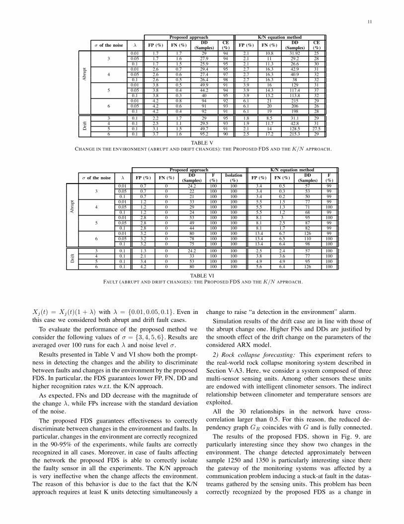
TABLE VCHANGE IN THE ENVIRONMENT (ABRUPT AND DRIFT CHANGES): THE PROPOSED FDS AND THEK/N APPROACH.

Proposed approach K/N equation method# of the noise " FP (%) FN (%) DD F Isolation FP (%) FN (%) DD F

(Samples) (%) (%) (Samples) (%)

Abrupt

30.01 0.7 0 24.2 100 100 3.4 0.5 57 990.05 0.7 0 22 100 100 3.4 0.3 53 990.1 0.7 0 21 100 100 3.4 0.2 50 99

40.01 1.2 0 33 100 100 5.5 1.5 77 990.05 1.2 0 29 100 100 5.5 1.3 71 1000.1 1.2 0 24 100 100 5.5 1.2 68 99

50.01 2.8 0 53 100 100 8.1 3 95 1000.05 2.8 0 49 100 100 8.1 2.5 87 990.1 2.8 0 44 100 100 8.1 1.7 82 99

60.01 3.2 0 80 100 100 13.4 6.7 126 990.05 3.2 0 78 100 100 13.4 6.5 110 1000.1 3.2 0 75 100 100 13.4 6.4 98 100

Drift 3 0.1 1.3 0 24.2 100 100 2.5 2.4 57 100

4 0.1 2.1 0 33 100 100 3.8 3.6 77 1005 0.1 3.4 0 53 100 100 4.9 4.9 95 1006 0.1 4.2 0 80 100 100 5.6 6.4 126 100

TABLE VIFAULT (ABRUPT AND DRIFT CHANGES): THE PROPOSED FDS AND THEK/N APPROACH.

Xj(t) = Xj(t)(1 + &) with & = {0.01, 0.05, 0.1}. Even inthis case we considered both abrupt and drift fault cases.To evaluate the performance of the proposed method we

consider the following values of $ = {3, 4, 5, 6}. Results areaveraged over 100 runs for each & and noise level $.Results presented in Table V and VI show both the prompt-

ness in detecting the changes and the ability to discriminatebetween faults and changes in the environment by the proposedFDS. In particular, the FDS guarantees lower FP, FN, DD andhigher recognition rates w.r.t. the K/N approach.As expected, FNs and DD decrease with the magnitude of

the change &, while FPs increase with the standard deviationof the noise.The proposed FDS guarantees effectiveness to correctly

discriminate between changes in the environment and faults. Inparticular, changes in the environment are correctly recognizedin the 90-95% of the experiments, while faults are correctlyrecognized in all cases. Moreover, in case of faults affectingthe network the proposed FDS is able to correctly isolatethe faulty sensor in all the experiments. The K/N approachis very ineffective when the change affects the environment.The reason of this behavior is due to the fact that the K/Napproach requires at least K units detecting simultaneously a

change to raise “a detection in the environment” alarm.Simulation results of the drift case are in line with those of

the abrupt change one. Higher FNs and DDs are justified bythe smooth effect of the drift change on the parameters of theconsidered ARX model.2) Rock collapse forecasting: This experiment refers to

the real-world rock collapse monitoring system described inSection V-A3. Here, we consider a system composed of threemulti-sensor sensing units. Among other sensors these unitsare endowed with intelligent clinometer sensors. The indirectrelationship between clinometer and temperature sensors areexploited.All the 30 relationships in the network have cross-

correlation larger than 0.5. For this reason, the reduced de-pendency graph GR coincides with G and is fully connected.The results of the proposed FDS, shown in Fig. 9, are

particularly interesting since they show two changes in theenvironment. The change detected approximately betweensample 1250 and 1350 is particularly interesting since therethe gateway of the monitoring systems was affected by acommunication problem inducing a stuck-at fault in the datas-treams gathered by the sensing units. This problem has beencorrectly recognized by the proposed FDS as a change in

12

200 400 600 800 1000 1200 1400 1600 1800 200010

15

20

Temperature

200 400 600 800 1000 1200 1400 1600 1800 2000

�6

�4

�2

x 10�3 Inclination

200 400 600 800 1000 1200 1400 1600 1800 20000

0.5

1

HMM CDT detections

200 400 600 800 1000 1200 1400 1600 1800 20000

0.5

1

Parity approach detections

Samples

Fig. 7. The application of the proposed method on real-world data comingfrom the rock collapse deployment. From top to bottom: (a) internal sensortemperature measurements, (b) clinometer measurements, (c) HMM-basedCDT detections and (d) Residual based detections.

the environment since all the units have been affected bythe change. Interestingly, a communication problem inducingchanges in all the network units can be associated with achange in the environment: no much more can be done here.The specific situation can be parallelized with the missing datachallenge, where the system provides constant-valued data aslong as the malfunction lasts. The second detection is labelledas a temporary environmental change and is in line with thedetection experiment described in Section V-A3.The K/N approach does not detect changes in the en-

vironment. This result emphasizes the limits of the K/Napproach which suffers from the fact that it requires at leastK relationships (i.e., in this case 15 relationships) to detect achange.3) Great Barrier Reef Ocean Observing System (GBROOS)

dataset: The GBROOS dataset refers to the temperaturemeasurements of six units belonging to the Great BarrierReef Ocean Observation System [42]. The considered unitsare deployed at the Heron Island, Queensland, Australia andthe acquisition campaign ranges from February 21 to March22, 2009. Interestingly, on March 9, 2009 a Category-4 cycloneaffected the deployment area. The dataset lasts approximately8400 samples and the cyclone occurs at about sample 4900.The sampling period is 5 mins.Here the training sequence is composed of 3000 samples

X1

Sensor 1

X11

Sensor 11

X2

Sensor 2

X12

Sensor 12

X3

Sensor 3

X13

Sensor 13

X4

Sensor 4

X14

Sensor 14

X5

Sensor 5

X15

Sensor 15

X6

Sensor 6

X16

Sensor 16

X7

Sensor 7

X17

Sensor 17

X8

Sensor 8

X18

Sensor 18

X9

Sensor 9

X19

Sensor 19

X10

Sensor 10

X20

Sensor 20

Fig. 8. The data generation graph of the recognition experiment on syntheticdata.

and the next 500 samples are used to compute the threshold.The reduced dependency graph is a fully-connected graph

since all 30 relationships produced cross-correlation higherthan !min. The results of the application of the proposed FDSon the GBROSS dataset are shown in Figure 10. We observethat1) the proposed FDS is correctly able to detect the occur-rence of a change in the environment approximately atsample 5000. Interestingly, the Australian Institute ofMarine Science (AIMS) asserts that the cyclone had notan immediate impact on the air temperature [42] andthis might be the reason of the delay in the detectionof the change in the environment. Obviously, the aimof the proposed system is not to detect the presenceof a cyclone (which is quite evident by itself) but todetect variations in the relationships within a set ofsensors. The GBROSS dataset well suits our needs sinceit provides both real measurements and a ground truthof an occurred change.

2) the change in the environment is only transient, as shownin Figure 10(a). This coincides with the evaluation ofAIMS which indicates that the effect of the cyclone onthe marine environment is only temporary and that theatmospheric conditions return to normal values within16 hours [42] after the transit of the cyclone.

Even in this case the K/N approach does not providesatisfactory results since it never happened that at least K (15)relationships raised an alarm at the same time.

VI. CONCLUSIONSThe paper introduces a cognitive FDS with novelties in

1) the design of a graph-based representation of the spa-tial/temporal relationships among measurements in a sensornetwork and, 2) a two-level hierarchical FDS exploiting suchtemporal and spatial relationships. The lower level of theFDS relies on a HMM-CDT to promptly detect changes in a

13

200 400 600 800 1000 1200 1400 1600 1800 200010

20

30

Temperature

200 400 600 800 1000 1200 1400 1600 1800 2000

�5

0

5

10

x 10�3 Inclination

200 400 600 800 1000 1200 1400 1600 1800 20000

0.5

1

Detection of environmental change (Ep) � Proposed FDS

200 400 600 800 1000 1200 1400 1600 1800 20000

0.5

1

Detection of environmental change (Ep) � K/N method

Samples

Unit 1Unit 2Unit 3

Unit 1Unit 2Unit 3

Fig. 9. Results on the data recorded by the rock collapse forecasting systemdeployed on the Alps. The two upper plots show the temperature and theclinometer measurements, while the lower plots presents the detection ofenvironmental changes (1: detection, 0: not detection) based on the proposedFDS and the K/N method.

relationship between two measurement datastreams, while theupper level exploits the graph-based functional representationof the network to discriminate among faults, changes in theenvironment and false positives induced by model bias. Theeffectiveness of the proposed solution has been evaluated onboth synthetic and real datasets.The FDS, which is here presented with the detection and

isolation phases, can be extended to consider also the identi-fication and accommodation ones.In fact, a set of HMMs can be trained to identify the

occurrence of a fault belonging to a-priori available faultdictionary. Once detected and verified by the upper level, theFDS could select the fault from the fault dictionary associatedwith the HMM showing the largest likelihood value.The accommodation phase aims at reducing the effects of a

change and adapting the system to the new working conditions.In case of faults, the affected sensor is removed from thereduced dependency graph and, possibly, substituted with itsvirtual representation (by exploiting the temporal and spatialredundancies with the other sensors). In case of changes inthe environment, the whole network representation (i.e., thereduced dependency graph and the HMMs) becomes obsoleteand must be retrained from up-to-date data, thus making theFDS adaptive over time. In case of fault detection induced bymodel bias, the corresponding HMM-CDT could be trained

1000 2000 3000 4000 5000 6000 7000 8000

26

28

30

32

34

36

Temperature

Samples

1000 2000 3000 4000 5000 6000 7000 80000

0.2

0.4

0.6

0.8

1

Detection of environmental change (Ep) # Proposed FDS

Samples

1000 2000 3000 4000 5000 6000 7000 80000

0.2

0.4

0.6

0.8

1

Detection of environmental change (Ep) # K/N method

Samples

Unit 1Unit 2Unit 3Unit 4Unit 5Unit 6

Fig. 10. Results on the GBROOS dataset. The upper plot presents thetemperature measurements of the six units. The following plots presentdetection of environmental changes (1: detection, 0: not detection) based onthe proposed FDS and the K/N method.

on a larger dataset.

ACKNOWLEDGMENTThis work was supported by the FP7 EU project i-Sense,

Making Sense of Nonsense, Contract No: INSFO-ICT-270428.

REFERENCES[1] R. Isermann, Fault-diagnosis systems: an introduction from fault detec-

tion to fault tolerance. Springer Verlag, 2006.[2] V. Venkatasubramanian, R. Rengaswamy, K. Yin, and S. N.

Kavuri, “A review of process fault detection and diagnosis: Part i:Quantitative model-based methods,” Computers Chemical Engineering,vol. 27, no. 3, pp. 293 – 311, 2003. [Online]. Available:http://www.sciencedirect.com/science/article/pii/S0098135402001606

[3] W. Shewhart, Economic control of quality of manufactured product.American Society for Quality, 1931, vol. 509.

[4] T. Lai, “Sequential analysis: some classical problems and new chal-lenges,” Statistica Sinica, vol. 11, no. 2, pp. 303–350, 2001.

[5] M. Basseville, I. Nikiforov et al., Detection of abrupt changes: theoryand application. Prentice Hall Englewood Cliffs, 1993, vol. 15.

[6] K. Goebel and W. Yan, “Correcting sensor drift and intermittency faultswith data fusion and automated learning,” Systems Journal, IEEE, vol. 2,no. 2, pp. 189–197, 2008.

[7] J. Frolik, M. Abdelrahman, and P. Kandasamy, “A confidence-basedapproach to the self-validation, fusion and reconstruction of quasi-redundant sensor data,” Instrumentation and Measurement, IEEE Trans-actions on, vol. 50, no. 6, pp. 1761–1769, Dec. 2001.

[8] T. Bohme, C. Cox, N. Valentin, and T. Denoeux, “Comparison ofautoassociative neural networks and kohonen maps for signal failuredetection and reconstruction,” Intelligent Engineering Systems throughArtificial Neural Networks, vol. 9, pp. 637–644, 1991.

14

[9] M. Napolitano, D. Windon, J. Casanova, M. Innocenti, and G. Silvestri,“Kalman filters and neural-network schemes for sensor validation inflight control systems,” Control Systems Technology, IEEE Transactionson, vol. 6, no. 5, pp. 596–611, Sept. 2002.

[10] T. Guo and J. Nurre, “Sensor failure detection and recovery by neuralnetworks,” in Neural Networks, 1991, IJCNN-91-Seattle InternationalJoint Conference on, vol. 1, 1991, pp. 221–226.

[11] R. Dunia, S. Qin, T. Edgar, and T. McAvoy, “Identification of faultysensors using principal component analysis,” AIChE Journal, vol. 42,no. 10, pp. 2797–2812, 1996.

[12] S. Wellington, J. Atkinson, and R. Sion, “Sensor validation and fusionusing the nadaraya-watson statistical estimator,” in Information Fusion,2002. Proceedings of the Fifth International Conference on, vol. 1, 2002,pp. 321–326.

[13] S. Huang and K. K. Tan, “Fault detection and diagnosis based onmodeling and estimation methods,” Neural Networks, IEEE Transactionson, vol. 20, no. 5, pp. 872 –881, May 2009.

[14] A. Trunov and M. Polycarpou, “Automated fault diagnosis in nonlinearmultivariable systems using a learning methodology,” Neural Networks,IEEE Transactions on, vol. 11, no. 1, pp. 91–101, Jan. 2000.

[15] E. Athanasopoulou and C. Hadjicostis, “Probabilistic approaches to faultdetection in networked discrete event systems,” Neural Networks, IEEETransactions on, vol. 16, no. 5, pp. 1042–1052, Sept. 2005.

[16] C. Rodriguez, S. Rementeria, J. Martin, A. Lafuente, J. Muguerza, andJ. Perez, “A modular neural network approach to fault diagnosis,” NeuralNetworks, IEEE Transactions on, vol. 7, no. 2, pp. 326 –340, Mar. 1996.

[17] Q. Liu, T. Chai, H. Wang, and S.-Z. J. Qin, “Data-based hybrid tensionestimation and fault diagnosis of cold rolling continuous annealingprocesses,” Neural Networks, IEEE Transactions on, vol. 22, no. 12,pp. 2284 –2295, Dec. 2011.

[18] R. Aggarwal, Q. Xuan, A. Johns, F. Li, and A. Bennett, “A novelapproach to fault diagnosis in multicircuit transmission lines usingfuzzy artmap neural networks,” Neural Networks, IEEE Transactionson, vol. 10, no. 5, pp. 1214 –1221, Sept. 1999.

[19] D. He, R. Li, J. Zhu, and M. Zade, “Data mining based full ceramicbearing fault diagnostic system using ae sensors,” Neural Networks,IEEE Transactions on, vol. 22, no. 12, pp. 2022–2031, Dec. 2011.

[20] M. Seera, C. P. Lim, D. Ishak, and H. Singh, “Fault detection anddiagnosis of induction motors using motor current signature analysisand a hybrid fmmcart model,” Neural Networks and Learning Systems,IEEE Transactions on, vol. 23, no. 1, pp. 97–108, Jan. 2012.

[21] D. Yang and H. Qi, “An effective decentralized nonparametric quickestdetection approach,” in Pattern Recognition (ICPR), 2010 20th Interna-tional Conference on, Aug. 2010, pp. 2278–2281.

[22] M. Chang, A. Terzis, and P. Bonnet, “Mote-based online anomalydetection using echo state networks,” in Proceedings of the 5th IEEEInternational Conference on Distributed Computing in Sensor Systems,ser. DCOSS ’09. Berlin, Heidelberg: Springer-Verlag, 2009, pp. 72–86.

[23] O. Obst, X. Wang, and M. Prokopenko, “Using echo state networks foranomaly detection in underground coal mines,” in Information Process-ing in Sensor Networks, 2008. IPSN ’08. International Conference on,april 2008, pp. 219 –229.

[24] M. Dong, D. Yang, Y. Kuang, D. He, S. Erdal, and D. Kenski, “Pm2.5concentration prediction using hidden semi-markov model-based timesseries data mining,” Expert Systems with Applications, vol. 36, no. 5,pp. 9046 – 9055, Jul. 2009.

[25] M. Dong and D. He, “Hidden semi-markov model-based methodologyfor multi-sensor equipment health diagnosis and prognosis,” EuropeanJournal of Operational Research, vol. 178, no. 3, pp. 858 – 878, May2007.

[26] ——, “A segmental hidden semi-markov model (hsmm)-based diagnos-tics and prognostics framework and methodology,” Mechanical Systemsand Signal Processing, vol. 21, no. 5, pp. 2248 – 2266, Jul. 2007.

[27] M. Maroti, B. Kusy, G. Simon, and A. Ledeczi, “Theflooding time synchronization protocol,” in Proceedings ofthe 2nd international conference on Embedded networkedsensor systems. ACM, 2004, pp. 39–49. [Online]. Available:http://portal.acm.org/citation.cfm?id=1031501

[28] C. Alippi, G. Boracchi, R. Camplani, A. Marullo, and M. Roveri, “Anhybrid monitoring system for the real-time processing of high frequencydata. part b: Software aspects,” Tech. Rep., 2011, internal Report.

[29] L. Ljung, “Convergence analysis of parametric identification methods,”Automatic Control, IEEE Transactions on, vol. 23, no. 5, pp. 770 – 783,Oct. 1978.

[30] L. Ljung and P. E. Caines, “Asymptotic normality of prediction errorestimators for approximate system models,” in Decision and Control

including the 17th Symposium on Adaptive Processes, 1978 IEEEConference on, vol. 17, Jan. 1978, pp. 927–932.

[31] G. Huang, Q. Zhu, and C. Siew, “Extreme learning machine: theory andapplications,” Neurocomputing, vol. 70, no. 1, pp. 489–501, Dec. 2006.

[32] B. Schrauwen, D. Verstraeten, and J. Van Campenhout, “An overviewof reservoir computing: theory, applications and implementations,”in Proceedings of the 15th European Symposium on ArtificialNeural Networks, 2007, pp. 471–482. [Online]. Available:http://citeseerx.ist.psu.edu/viewdoc/summary?doi=10.1.1.95.1215

[33] D. A. Reynolds, T. F. Quatieri, and R. B. Dunn, “Speakerverification using adapted gaussian mixture models,” Digital SignalProcessing, vol. 10, no. 1-3, pp. 19–41, 2000. [Online]. Available:http://www.sciencedirect.com/science/article/pii/S1051200499903615

[34] L. R. Rabiner and B. H. Juang, “An introduction to hidden markovmodels,” IEEE ASSP Magazine, pp. 4–15, Jan. 1986.

[35] R. Durbin, S. R. Eddy, A. Krogh, and G. Mitchison,Biological Sequence Analysis: Probabilistic Models of Proteinsand Nucleic Acids. Cambridge University Press, Jul. 1998. [Online].Available: http://www.amazon.ca/exec/obidos/redirect?tag=citeulike09-20&amp;path=ASIN/0521629713

[36] C. Alippi, G. Boracchi, and M. Roveri, “On-line reconstruction of miss-ing data in sensor/actuator networks by exploiting temporal and spatialredundancy,” in Neural Networks (IJCNN), The 2012 International JointConference on. IEEE, 2012, pp. 1–8.

[37] S. Mirsaidi, G. Fleury, and J. Oksman, “Lms-like ar modeling in thecase of missing observations,” Signal Processing, IEEE Transactionson, vol. 45, no. 6, pp. 1574–1583, 1997.

[38] F. Ding and J. Ding, “Least-squares parameter estimation for systemswith irregularly missing data,” International Journal of Adaptive Controland Signal Processing, vol. 24, no. 7, pp. 540–553, 2010.

[39] Torch machine learning library. [Online]. Available: http://www.torch.ch/[40] J. Quevedo, V. Puig, G. Cembrano, J. Blanch, J. Aguilar, D. Saporta,

G. Benito, M. Hedo, and A. Molina, “Validation and reconstruction offlow meter data in the Barcelona water distribution network,” ControlEngineering Practice, vol. 18, pp. 640–651, Jun. 2010.

[41] C. Alippi, G. Boracchi, A. Marullo, and M. Roveri, “A step towardsthe prediction of a rock collapse: analysis of micro-acoustic bursts,” inSensors, 2011 IEEE, Oct. 2011, pp. 1273–1276.

[42] J. Bezdek, S. Rajasegarar, M. Moshtaghi, C. Leckie, M. Palaniswami,and T. Havens, “Anomaly detection in environmental monitoring net-works [application notes],” Computational Intelligence Magazine, IEEE,vol. 6, no. 2, pp. 52–58, May 2011.