A Color Image Denoising By Hybrid Filter for Mixed Noiseinpressco.com/wp-content/uploads/2015/05/Paper141565-15721.pdfA Color Image Denoising By Hybrid Filter for Mixed Noise ... The

International Journal of Current Engineering and Technology E-ISSN 2277 – 4106, P-ISSN 2347 – 5161 ©2015 INPRESSCO®, All Rights Reserved Available at http://inpressco.com/category/ijcet

Research Article

1565| International Journal of Current Engineering and Technology, Vol.5, No.3 (June 2015)

A Color Image Denoising By Hybrid Filter for Mixed Noise Prateek Kumar†* and Sandeep Kumar Agarwal†

†Department of Electronics Communication Engineering, Rustamji Institute of Technology, BSF Academy, Tekanpur, Gwalior (M.P.), S-4 Sarika-Nagar, Thatipur, Gwalior, India Accepted 03 May 2015, Available online 05 May 2015, Vol.5, No.3 (June 2015)

Abstract Image denoising is the manipulation of the image data to produce a visually high quality image. At present there are a variety of methods to remove noise from digital images. There are different types of filters like mean filter, median filter, bilateral filter, wiener filter etc. to remove a single type of noise such as salt and pepper noise, speckle noise, Gaussian noise etc. But if the image is corrupted by mixed type of noise then these filters do not remove the noise exactly. Here a White Flower image has been taken for denoising purpose. Noisy image is first denoised by wavelet denoising technique, median filter, wiener filter and bilateral filter separately. Last it is denoised by hybrid filter. A Hybrid filter is composite of various filters to remove of mixed type of noise from a digital image. Hybridization of median filter, wiener filter and bilateral filter for denoising of variety of noisy images is presented in this paper. The comparison between denoised images is taken in terms of performance parameters such as MSE (mean square error), PSNR (peak signal to noise ratio), RMSE (root mean square error), SNR (signal to noise ratio) and SSIM (structural similarity index).The software used for simulation is MATLAB R2014a (8.3.0.532). Keywords: Salt-and-pepper noise, Gaussian noise, speckle noise, wavelet denoising, median filter, bilateral filter, wiener filter, PSNR, SNR, RMSE, MSE, SSIM. 1. Introduction

1 Image denoising restores the details of an image by removing unwanted noise. Digital images become noisy when these are acquired by a defective sensor or when these are transmitted through a faulty channel (Er. Amita Kumari, et al, 2014). Having a good knowledge about the noise present in the image is important in selecting a suitable denoising algorithm (vijayalakshmi, et al, 2014). The denoising methods include Gaussian filtering and Wiener filtering etc. However, these methods lose fine details of the image which leads to blur in the image. (Er. Amita Kumari, et al, 2014). Impulsive noises are commonly found in the sensor or transmission channel during the acquisition and transfer procedure. Salt-and-pepper noise is a typical kind of impulsive noise. It is well known that linear filtering techniques fail when the noise is non-additive and are not effective in removing impulse noise. The nonlinear filter algorithms are often adopted for the salt-and-pepper noise removal. The widely used nonlinear digital filter is median filter. Median filter is known for their capability to remove impulse noise. The main drawback of a standard median filter (SMF) is that it is effective only for low noise densities. At high noise densities, SMFs often exhibit blurring for

*Corresponding author: Prateek Kumar

large window sizes and insufficient noise suppression for small window sizes. Hybrid filter consists the properties two or more filters. Hybrid filter can remove the additive, multiplicative as well as mixed noise effectively and can produce denoised image of higher quality in comparison to single filtering technique. Noise is a random variation of image Intensity and visible as grains in the image. It may arise in the image as effects of basic physics-like photon nature of light or thermal energy of heat inside the image sensors(Mario Mastriani, 2009 ).

Here we are discussing about three types of noise and their effect on the image signal.

1) Gaussian noise 2) Speckle noise 3) Salt-and-pepper noise This noise model is additive in nature. Additive white Gaussian noise (AWGN) can be caused by poor quality image acquisition, noisy environment or internal noise in communication channels. Gaussian noise is statistical noise having a probability density function (PDF) equal to that of the normal distribution , which is also known as the Gaussian distribution(Priyanka Kamboj, et al, 2013). Gaussian noise is uniformly distributed over the signal. It means that each pixel in

Prateek Kumar et al A Color Image Denoising By Hybrid Filter for Mixed Noise


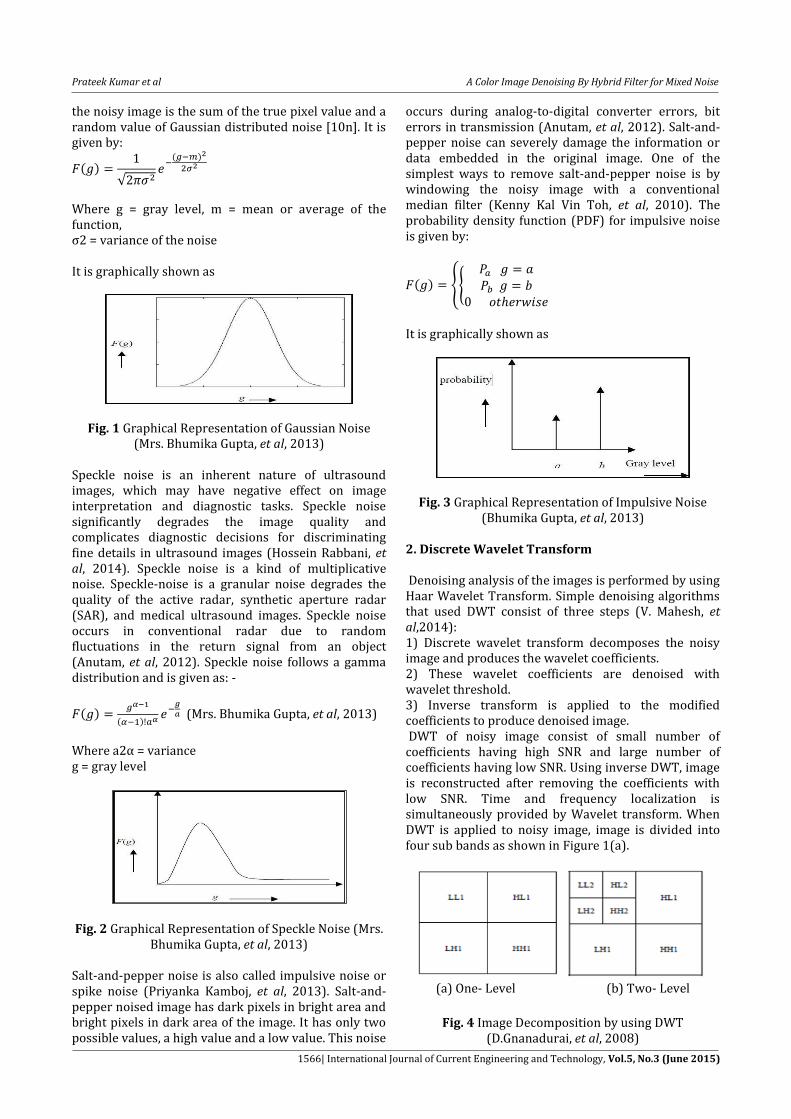
the noisy image is the sum of the true pixel value and a random value of Gaussian distributed noise [10n]. It is given by:

( )

√ ( )

Where g = gray level, m = mean or average of the function, σ2 = variance of the noise It is graphically shown as

Fig. 1 Graphical Representation of Gaussian Noise (Mrs. Bhumika Gupta, et al, 2013)

Speckle noise is an inherent nature of ultrasound images, which may have negative effect on image interpretation and diagnostic tasks. Speckle noise significantly degrades the image quality and complicates diagnostic decisions for discriminating fine details in ultrasound images (Hossein Rabbani, et al, 2014). Speckle noise is a kind of multiplicative noise. Speckle-noise is a granular noise degrades the quality of the active radar, synthetic aperture radar (SAR), and medical ultrasound images. Speckle noise occurs in conventional radar due to random fluctuations in the return signal from an object (Anutam, et al, 2012). Speckle noise follows a gamma distribution and is given as: -

( )

( )

(Mrs. Bhumika Gupta, et al, 2013)

Where a2α = variance g = gray level

Fig. 2 Graphical Representation of Speckle Noise (Mrs. Bhumika Gupta, et al, 2013)

Salt-and-pepper noise is also called impulsive noise or spike noise (Priyanka Kamboj, et al, 2013). Salt-and-pepper noised image has dark pixels in bright area and bright pixels in dark area of the image. It has only two possible values, a high value and a low value. This noise

occurs during analog-to-digital converter errors, bit errors in transmission (Anutam, et al, 2012). Salt-and-pepper noise can severely damage the information or data embedded in the original image. One of the simplest ways to remove salt-and-pepper noise is by windowing the noisy image with a conventional median filter (Kenny Kal Vin Toh, et al, 2010). The probability density function (PDF) for impulsive noise is given by:

( ) {{

It is graphically shown as

Fig. 3 Graphical Representation of Impulsive Noise (Bhumika Gupta, et al, 2013)

2. Discrete Wavelet Transform

Denoising analysis of the images is performed by using Haar Wavelet Transform. Simple denoising algorithms that used DWT consist of three steps (V. Mahesh, et al,2014): 1) Discrete wavelet transform decomposes the noisy image and produces the wavelet coefficients. 2) These wavelet coefficients are denoised with wavelet threshold. 3) Inverse transform is applied to the modified coefficients to produce denoised image. DWT of noisy image consist of small number of coefficients having high SNR and large number of coefficients having low SNR. Using inverse DWT, image is reconstructed after removing the coefficients with low SNR. Time and frequency localization is simultaneously provided by Wavelet transform. When DWT is applied to noisy image, image is divided into four sub bands as shown in Figure 1(a).

(a) One- Level (b) Two- Level

Fig. 4 Image Decomposition by using DWT

(D.Gnanadurai, et al, 2008)



These sub bands are formed by separable applications of horizontal and vertical filters. Coefficients that are represented as sub bands LH1, HL1 and HH1 are detail images while coefficients are represented as sub band LL1 is approximation image (D.Gnanadurai, et al, 2008). The LL1 sub band is further decomposed to obtain the next level of wavelet coefficients as shown in Fig. 1(b). LL1 is called the approximation sub band as it provides the image as like as original image. It comes from low pass filtering in both directions. The other bands are called detail sub bands. The filters L and H as shown in Figure 2. are one dimensional low pass filter (LPF) and high pass filter (HPF) for image decomposition. HL1 is called the horizontal fluctuation as it comes from low pass filtering in vertical direction and high pass filtering in horizontal direction. LH1 is called vertical fluctuation as it comes from high pass filtering in vertical direction and low pass filtering in horizontal direction. HH1 is called diagonal fluctuation as it comes from high pass filtering in both the directions. LL1 is decomposed into 4 sub bands LL2, LH2, HL2 and HH2. The process is carried until the fifth decomposition is reached. After L decompositions a total of D (L) =3*L+1 sub bands are obtained. Therefore after 5 decompositions D (5) = 3*5+1 = 16 sub bands are obtained. The decomposed image can be reconstructed by inverse discrete wavelet transform as shown in Figure 3. Here, the filters L and H represent low pass and high pass reconstruction filters respectively.

Fig.5 Wavelet Filter bank for one-level Image Decomposition (D.Gnanadurai, et al, 2008)

Fig. 6 Wavelet Filter bank for one-level Image Reconstruction (D.Gnanadurai, et al, 2008)

3. Median Filter

Median filtering has a good edge preserving ability, and

does not introduce new pixel values to the processed

image (Wei Fan, et al, 2015). The Median filter is a non-

linear smoothing technique that reduces the blurring of

edges; here the idea is to replace the current point in

the image by the median of the brightness in its

neighborhood. The median of the brightness in the

neighborhood is not affected by individual noise

spikes. The median filter eliminates impulse noise

efficiently. Since median filtering does not blur edges

much, it can be applied iteratively. One of the major

problems with the median filter is that it is relatively

expensive and is hard to compute. It is essential to sort

all the values in the neighborhood into numerical in

order to find out the median value which is relatively

slow (Vijayalakshmi, et al, 2014). Median filter is based

on the following steps: (Er. Amita Kumari, et al, 2014)

1) It checks for pixels that are noisy in the image.

2) For each such pixel P, a window of size 5×5 around

the pixel P is taken.

3) Find the absolute differences between the pixel P

and the surrounding pixels.

4) The arithmetic mean (AM) of the differences for a

given pixel p is computed.

5) The AM is then compared with the ―threshold to

detect whether the pixel p is informative or corruptive.

a) If AM is greater than or equal to the threshold the

pixel is considered noisy.

b) Otherwise the pixel is considered as information.

The filter fails to perform well at higher noise densities.

When noise density is high it is highly unlikely that

there might be more informative pixels than corruptive

pixels.

4. Weiner Filter

Wiener filters are characterized by the following: a) Assumption: signal and (additive) noise are stationary linear random processes with known spectral characteristics. b) Requirement: the filter must be physically realizable, i.e. causal (this requirement can be dropped, resulting in a non-causal solution) c) Performance criteria: minimum mean-square error (Ashok Kumar Nagawat, et al, 2010). Weiner filtration gives an estimate of the original uncorrupted image with minimal mean square error; the optimal estimate is in general a non-linear function of the corrupted image.



The function can be written by,

( ) [ ( )

( ) [ ( )

( )]] ( ) (Rekha Rani, et al,

2012) where ( ) is the degradation function ( ) is its conjugate complex and ( ) is the degraded image. Functions ( ) and ( )are power spectra of the original image and the noise. (Vijayalakshmi, et al, 2014). 5. Bilateral filtering

The bilateral filtering is an edge-preserving smoothing

technique which effectively blurs the image but

maintains the sharpness of edges (Jong-Woo Han, et al,

2010). The bilateral filtering was introduced by Tomasi

and Manduchi. It is achieved by the combinations of the

two Gaussian filters. One filter works in spatial domain

and the second filter works in intensity domain. It is a

non-linear filter where the output is a weighted

average of the input. The output of the bilateral filter

for a pixel s is defined as follows: (Moussa Olfa, et al,

2014)

( )

( )∑ ( )( )

Where k(s) is a normalization term:

( ) ∑ ( ) ( )

Where f uses a Gaussian in the spatial domain which is

represents the domain filter and g uses a Gaussian in

the intensity domain which represents the range filter.

Domain filtering can be expressed mathematically as:

( )

( )∑ ( )

Where ( ) ‖ ‖

f(p-s) measures the

spatial closeness between the neighborhood center s

and a nearby point p and:

( ) ∑ ( )

Range filtering is defined as follows:

( )

( )∑ ( )

Where ( ) ‖ ‖

( ) measures the photometric similarity

between the center pixel s and its nearby point p. The

normalized constant in this case is:

( ) ∑ ( )

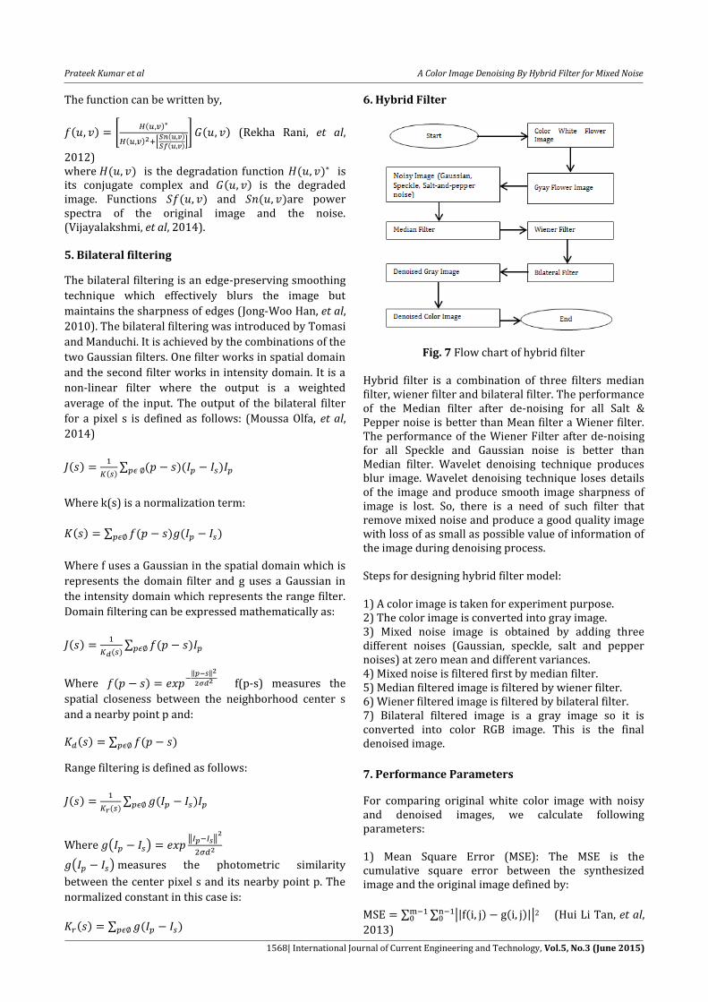
6. Hybrid Filter

Fig. 7 Flow chart of hybrid filter Hybrid filter is a combination of three filters median filter, wiener filter and bilateral filter. The performance of the Median filter after de-noising for all Salt & Pepper noise is better than Mean filter a Wiener filter. The performance of the Wiener Filter after de-noising for all Speckle and Gaussian noise is better than Median filter. Wavelet denoising technique produces blur image. Wavelet denoising technique loses details of the image and produce smooth image sharpness of image is lost. So, there is a need of such filter that remove mixed noise and produce a good quality image with loss of as small as possible value of information of the image during denoising process. Steps for designing hybrid filter model: 1) A color image is taken for experiment purpose. 2) The color image is converted into gray image. 3) Mixed noise image is obtained by adding three different noises (Gaussian, speckle, salt and pepper noises) at zero mean and different variances. 4) Mixed noise is filtered first by median filter. 5) Median filtered image is filtered by wiener filter. 6) Wiener filtered image is filtered by bilateral filter. 7) Bilateral filtered image is a gray image so it is converted into color RGB image. This is the final denoised image.

7. Performance Parameters

For comparing original white color image with noisy and denoised images, we calculate following parameters: 1) Mean Square Error (MSE): The MSE is the cumulative square error between the synthesized image and the original image defined by:

∑ ∑ || ( ) ( )||

2 (Hui Li Tan, et al,

2013)



Where, f is the original image and g is the synthesized image. MSE should be as low as possible. 2) Peak signal to Noise ratio (PSNR): PSNR is the ratio between maximum possible power of a signal and the power of distorting noise which affects the quality of the original signal (Anutam, et al, 2012). It is defined by:

( )

√ ( ).

Where MAXF is the maximum signal value that exists in our original image. PSNR should be as high as possible. 3) Root mean square error (RMSE): It measures of the differences between value predicted by a model or an estimator and the values actually observed. It is the square root of mean square error. RMSE should be as low as Possible.

√ 4) Structural Similarity Index (SSIM): It is a method for measuring the similarity between two images (Mehul P. Sampat, et al, 2009). The SSIM measure the image quality based on an initial distortion-free image as reference.

( )( )

(

)(

)

the average of x; the average of y; the variance of x; the variance of y; the covariance of x and y; = (k1L)2 and = (k2L)2 are two variables to stabilize the division with weak denominator. L the dynamic range of the pixel-values k1 = 0.01 and k2 = 0.03 by default. The resultant SSIM index is a decimal value between -1 and 1, and value 1 is only reachable in the case of two identical sets of data. 5) Signal to noise ratio (SNR): Signal-to-noise ratio is defined as the power ratio between a signal (meaningful information) and the noise (unwanted signal) It should be as low as possible:

(Yu-Hsin, et al, 2014)

8. Result

(a) (b)

(c) (d)

(e) (f)

(g) (h)

(i)

Fig. 8 (a) Original White color flower (b) Gray flower

Image (c) Image obtained after adding all three noises (d) Image obtained after denoising by wavelet

technique (e) Image obtained after filtering by wiener filter (f) Image obtained after filtering by median filter (g) Image obtained after filtering by bilateral filter (h) Image obtained after filtering by hybrid filter (i) Image

obtained after converting gray hybrid filtered into a color image.

Figure 6 represents the original white color image, mixed noise image and filtered images by different filters. Performance parameter calculates the performance of the filters. PSNR, SNR, and SSIM should be high for a denoised image as compare to noisy image while RMSE and MSE should be low for a denoised image as compare to noisy image. All three noises are added one by one at zero mean and different variances on the white flower image to produce a mixed noise image. SNR, PSNR, SSIM of the original image decreases and MSE and RMSE of the original image increases as the noises are added on the



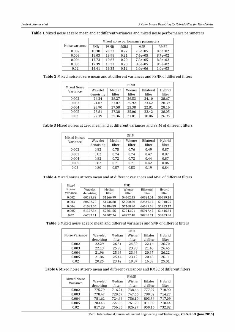
Table 1 Mixed noise at zero mean and at different variances and mixed noise performance parameters

Noise variance

Mixed noise performance parameters

SNR PSNR SSIM MSE RMSE 0.002 18.38 20.33 0.22 7.5e+05 8.6e+02 0.003 18.03 19.98 0.21 7.6e+05 8.7e+02 0.004 17.73 19.67 0.20 7.8e+05 8.8e+02 0.005 17.39 19.33 0.20 8.0e+05 8.9e+02 0.02 14.41 16.35 0.12 1.0e+06 1.0e+03

Table 2 Mixed noise at zero mean and at different variances and PSNR of different filters

Mixed Noise Variance

PSNR

Wavelet denoising

Median filter

Wiener filter

Bilateral filter

Hybrid filter

0.002 24.24 28.27 26.53 24.10 28.67 0.003 24.07 27.87 25.92 23.42 28.39 0.004 23.90 27.58 25.38 22.81 28.16 0.005 23.81 27.38 25.06 22.42 28.05 0.02 22.19 25.36 21.81 18.06 26.95

Table 3 Mixed noises at zero mean and at different variances and SSIM of different filters

Mixed Noises Variance

SSIM

Wavelet denoising

Median filter

Wiener filter

Bilateral filter

Hybrid filter

0.002 0.82 0.75 0.76 0.49 0.87

0.003 0.82 0.74 0.74 0.47 0.87 0.004 0.82 0.72 0.72 0.44 0.87

0.005 0.82 0.71 0.71 0.42 0.86

0.02 0.80 0.57 0.53 0.19 0.84

Table 4 Mixed noises at zero mean and at different variances and MSE of different filters

Mixed Noises

variance

MSE

Wavelet denoising

Median filter

Wiener filter

Bilateral filter

Hybrid filter

0.002 60135.82 51266.99 54562.45 60524.01 50539.14

0.003 60602.70 51936.88 55900.50 62540.17 51018.95

0.004 61093.06 52484.89 57168.90 64539.58 51423.17

0.005 61377.36 52861.55 57943.91 65917.42 51616.54

0.02 66797.11 57207.74 68272.48 90280.71 53703.80

Table 5 Mixed noise at zero mean and different variances and SNR of different filters

Noise Variance SNR

Wavelet denoising

Median filter

Wiener filter

Bilateral filter

Hybrid filter

0.002 22.29 26.31 24.59 22.16 26.70 0.003 22.13 25.93 23.98 21.48 26.45 0.004 21.96 25.63 23.43 20.87 26.22 0.005 21.86 25.44 23.12 20.48 26.11 0.02 20.25 23.42 19.87 16.09 25.01

Table 6 Mixed noise at zero mean and different variances and RMSE of different filters

Mixed Noise Variance

RMSE

Wavelet denoising

Median filter

Wiener filter

Bilateral filter

Hybrid filter

0.002 775.79 716.24 738.66 777.97 710.90 0.003 778.47 720.67 747.66 790.82 714.27 0.004 781.62 724.64 756.10 803.36 717.09 0.005 783.43 727.05 761.20 811.89 718.44 0.02 817.29 756.35 826.27 950.16 732.82



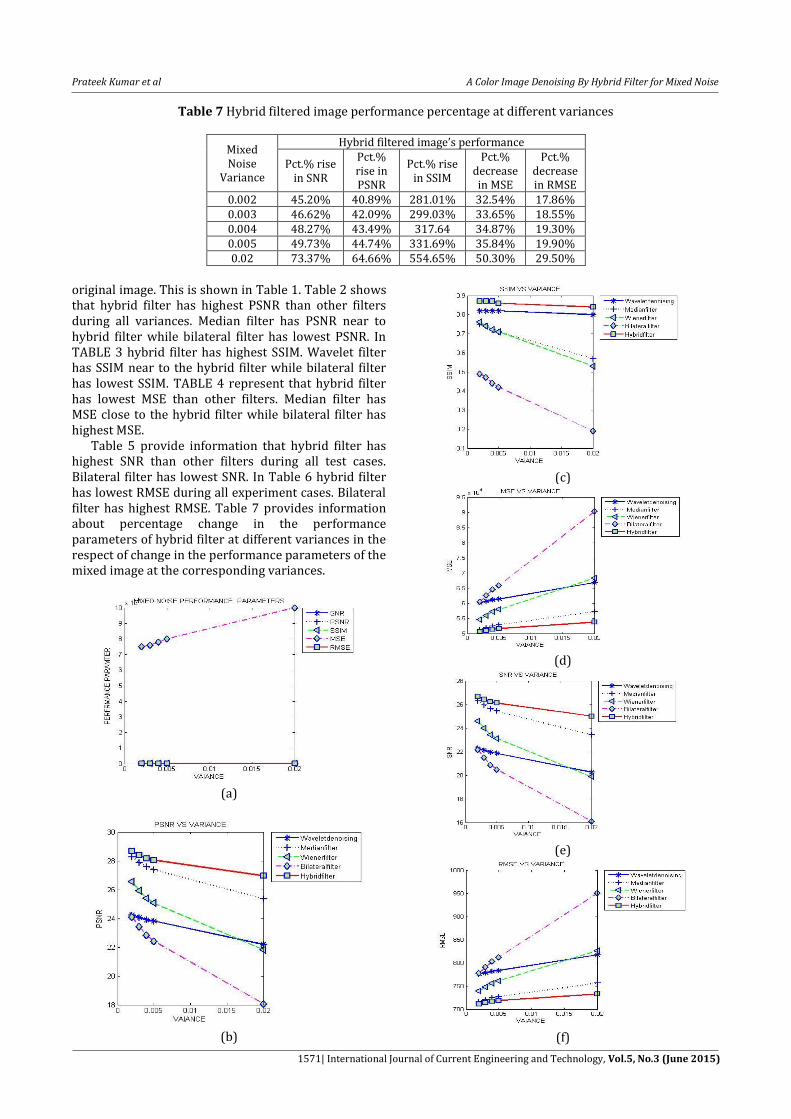
Table 7 Hybrid filtered image performance percentage at different variances

Mixed Noise

Variance

Hybrid filtered image’s performance

Pct.% rise in SNR

Pct.% rise in PSNR

Pct.% rise in SSIM

Pct.% decrease in MSE

Pct.% decrease in RMSE

0.002 45.20% 40.89% 281.01% 32.54% 17.86% 0.003 46.62% 42.09% 299.03% 33.65% 18.55% 0.004 48.27% 43.49% 317.64 34.87% 19.30% 0.005 49.73% 44.74% 331.69% 35.84% 19.90% 0.02 73.37% 64.66% 554.65% 50.30% 29.50%

original image. This is shown in Table 1. Table 2 shows that hybrid filter has highest PSNR than other filters during all variances. Median filter has PSNR near to hybrid filter while bilateral filter has lowest PSNR. In TABLE 3 hybrid filter has highest SSIM. Wavelet filter has SSIM near to the hybrid filter while bilateral filter has lowest SSIM. TABLE 4 represent that hybrid filter has lowest MSE than other filters. Median filter has MSE close to the hybrid filter while bilateral filter has highest MSE. Table 5 provide information that hybrid filter has highest SNR than other filters during all test cases. Bilateral filter has lowest SNR. In Table 6 hybrid filter has lowest RMSE during all experiment cases. Bilateral filter has highest RMSE. Table 7 provides information about percentage change in the performance parameters of hybrid filter at different variances in the respect of change in the performance parameters of the mixed image at the corresponding variances.

(a)

(b)

(c)

(d)

(e)

(f)



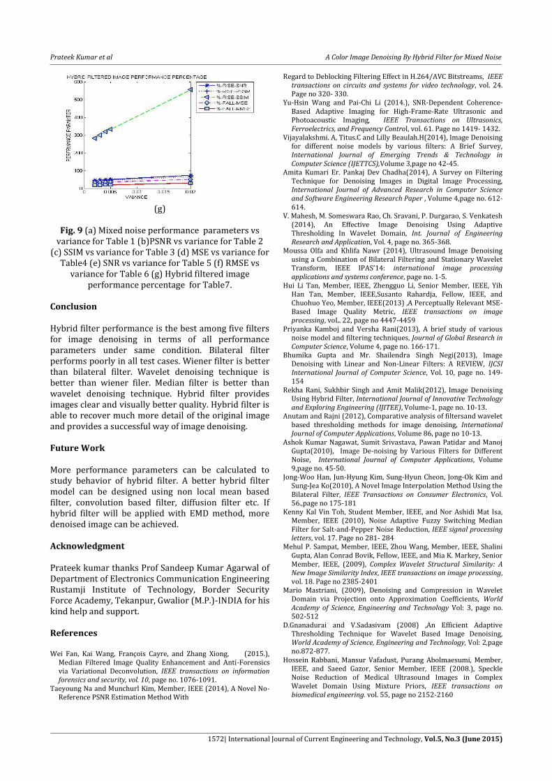
(g)

Fig. 9 (a) Mixed noise performance parameters vs

variance for Table 1 (b)PSNR vs variance for Table 2 (c) SSIM vs variance for Table 3 (d) MSE vs variance for

Table4 (e) SNR vs variance for Table 5 (f) RMSE vs variance for Table 6 (g) Hybrid filtered image

performance percentage for Table7.

Conclusion Hybrid filter performance is the best among five filters for image denoising in terms of all performance parameters under same condition. Bilateral filter performs poorly in all test cases. Wiener filter is better than bilateral filter. Wavelet denoising technique is better than wiener filer. Median filter is better than wavelet denoising technique. Hybrid filter provides images clear and visually better quality. Hybrid filter is able to recover much more detail of the original image and provides a successful way of image denoising. Future Work More performance parameters can be calculated to study behavior of hybrid filter. A better hybrid filter model can be designed using non local mean based filter, convolution based filter, diffusion filter etc. If hybrid filter will be applied with EMD method, more denoised image can be achieved. Acknowledgment Prateek kumar thanks Prof Sandeep Kumar Agarwal of Department of Electronics Communication Engineering Rustamji Institute of Technology, Border Security Force Academy, Tekanpur, Gwalior (M.P.)-INDIA for his kind help and support. References Wei Fan, Kai Wang, François Cayre, and Zhang Xiong, (2015.),

Median Filtered Image Quality Enhancement and Anti-Forensics via Variational Deconvolution, IEEE transactions on information forensics and security, vol. 10, page no. 1076-1091.

Taeyoung Na and Munchurl Kim, Member, IEEE (2014), A Novel No-Reference PSNR Estimation Method With

Regard to Deblocking Filtering Effect in H.264/AVC Bitstreams, IEEE transactions on circuits and systems for video technology, vol. 24. Page no 320- 330.

Yu-Hsin Wang and Pai-Chi Li (2014.), SNR-Dependent Coherence-Based Adaptive Imaging for High-Frame-Rate Ultrasonic and Photoacoustic Imaging, IEEE Transactions on Ultrasonics, Ferroelectrics, and Frequency Control, vol. 61. Page no 1419- 1432.

Vijayalakshmi. A, Titus.C and Lilly Beaulah.H(2014), Image Denoising for different noise models by various filters: A Brief Survey, International Journal of Emerging Trends & Technology in Computer Science (IJETTCS),Volume 3,page no 42-45.

Amita Kumari Er. Pankaj Dev Chadha(2014), A Survey on Filtering Technique for Denoising Images in Digital Image Processing, International Journal of Advanced Research in Computer Science and Software Engineering Research Paper , Volume 4,page no. 612-614.

V. Mahesh, M. Someswara Rao, Ch. Sravani, P. Durgarao, S. Venkatesh (2014), An Effective Image Denoising Using Adaptive Thresholding In Wavelet Domain, Int. Journal of Engineering Research and Application, Vol. 4, page no. 365-368.

Moussa Olfa and Khlifa Nawr (2014), Ultrasound Image Denoising using a Combination of Bilateral Filtering and Stationary Wavelet Transform, IEEE IPAS’14: international image processing applications and systems conference, page no. 1-5.

Hui Li Tan, Member, IEEE, Zhengguo Li, Senior Member, IEEE, Yih Han Tan, Member, IEEE,Susanto Rahardja, Fellow, IEEE, and Chuohuo Yeo, Member, IEEE(2013) ,A Perceptually Relevant MSE-Based Image Quality Metric, IEEE transactions on image processing, voL. 22, page no 4447-4459

Priyanka Kamboj and Versha Rani(2013), A brief study of various noise model and filtering techniques, Journal of Global Research in Computer Science, Volume 4, page no. 166-171.

Bhumika Gupta and Mr. Shailendra Singh Negi(2013), Image Denoising with Linear and Non-Linear Filters: A REVIEW, IJCSI International Journal of Computer Science, Vol. 10, page no. 149-154

Rekha Rani, Sukhbir Singh and Amit Malik(2012), Image Denoising Using Hybrid Filter, International Journal of Innovative Technology and Exploring Engineering (IJITEE), Volume-1, page no. 10-13.

Anutam and Rajni (2012), Comparative analysis of filtersand wavelet based thresholding methods for image denoising, International Journal of Computer Applications, Volume 86, page no 10-13.

Ashok Kumar Nagawat, Sumit Srivastava, Pawan Patidar and Manoj Gupta(2010), Image De-noising by Various Filters for Different Noise, International Journal of Computer Applications, Volume 9,page no. 45-50.

Jong-Woo Han, Jun-Hyung Kim, Sung-Hyun Cheon, Jong-Ok Kim and Sung-Jea Ko(2010), A Novel Image Interpolation Method Using the Bilateral Filter, IEEE Transactions on Consumer Electronics, Vol. 56.,page no 175-181

Kenny Kal Vin Toh, Student Member, IEEE, and Nor Ashidi Mat Isa, Member, IEEE (2010), Noise Adaptive Fuzzy Switching Median Filter for Salt-and-Pepper Noise Reduction, IEEE signal processing letters, vol. 17. Page no 281- 284

Mehul P. Sampat, Member, IEEE, Zhou Wang, Member, IEEE, Shalini Gupta, Alan Conrad Bovik, Fellow, IEEE, and Mia K. Markey, Senior Member, IEEE, (2009), Complex Wavelet Structural Similarity: A New Image Similarity Index, IEEE transactions on image processing, vol. 18. Page no 2385-2401

Mario Mastriani, (2009), Denoising and Compression in Wavelet Domain via Projection onto Approximation Coefficients, World Academy of Science, Engineering and Technology Vol: 3, page no. 502-512

D.Gnanadurai and V.Sadasivam (2008) ,An Efficient Adaptive Thresholding Technique for Wavelet Based Image Denoising, World Academy of Science, Engineering and Technology, Vol: 2,page no.872-877.

Hossein Rabbani, Mansur Vafadust, Purang Abolmaesumi, Member, IEEE, and Saeed Gazor, Senior Member, IEEE (2008.), Speckle Noise Reduction of Medical Ultrasound Images in Complex Wavelet Domain Using Mixture Priors, IEEE transactions on biomedical engineering. vol. 55, page no 2152-2160

Documents

A Color Image Denoising By Hybrid Filter for Mixed Noiseinpressco.com/wp-content/uploads/2015/05/Paper141565-15721.pdfA Color Image Denoising By Hybrid Filter for Mixed Noise ... The