Embed Size (px)
Citation preview
Computers & Geosciences Vol. 19, No. 7, pp. 873 886, 1993 0098-3004/93 $6.00 + 0.00 Printed in Great Britain. All rights reserved Copyright ,,~" 1993 Pergamon Press Ltd
A COMBINATORIAL ALGORITHM FOR THE OPTIMIZATION OF REFRACTION SEISMICS D A T A
INVERSION
STEFANO MICCIANCIO lstituto di Fisica, Facoltfi di Scienze, Universit~i di Palermo, via Archirafi 36, 1-90123 Palermo, Italy
(Received 5 May 1992; accepted 16 November 1992; revised 2 February 1993)
Al~tract--The problem of data inversion in refraction seismics can be split in two parts: data first must be preprocessed in order to determine the travel-time curve; this essentially is a geometrical problem, complicated, however, by its pattern recognition aspects. Once the geometrical problem is solved, the second part, the inversion proper, is straightforward, as the soil layering model can be calculated according to well-known algorithms. The more difficult part of the problem is the former, which implies a type of pattern recognition; because of this type of difficulty, the geometrical part of the problem usually is committed to the skill of a human operator. This paper describes an algorithm exploiting combinatorial optimization techniques to automatize the pattern recognition part of the problem of data inversion in refraction seismics. The listing of a Pascal source program, implementing the algorithm proposed, is included.
Key Words: Refraction seismics, Computer-aided data analysis, Combinatorial optimization.
INTRODUCTION
Almost always, raw experimental data yield useful information only after some processing. Numerical processing now is deputed to computers, but raw data, before being processed numerically, may need some preprocessing that, although apparently simple, in many instances cannot be automated easily, and must be performed by a skilled human operator.
One such situation is encountered in shallow, limited area refraction seismics, where two sets of time-distance pairs (forward and reverse survey) first must be divided in subsets containing the arrivals from the same refractor. In the assumption of plane- tilted layer interfaces, the problem is to approximate the experimental travel-time versus distance data with a set of straight segments; then the parameters defining the segments are used to compute the strati- graphic parameters according to well-known algor- ithms. Part of the job is a typical pattern recognition task that could be performed easily "by eye", were it not for constraints that interrelate the two curves and that are not handled easily "by eye", as we shall see.
This paper describes an application of combinato- rial optimization techniques to the preprocessing of data in the inversion problem encountered in refrac- tion seismics. The algorithm described here defines an objective quantitative parameter measuring the good- ness of a straight segment approximation of a pair of travel-time versus distance curves. This parameter is used to obtain "the best" stratigraphic parameters consistent with the data of a refraction seismic sur- vey. The entire procedure can be made fully auto-
matic. A Pascal source code implementing it is reported in the Appendix.
Let D = {(X~, ti), i = 1...N} be a set of experimen- tal data from a refraction seismic survey, where the x:s are the distances of the geophones from the shooting point, and the t~'s are the time of first arrival of the signal to the ith geophone. It is well known that in the approximation of homogeneous and sharply bounded layers, separated by plane inter- faces, with the speed of sound monotonically increas- ing downward from one layer to other, the points of the set D will be arranged in M subsets, each of which defines a straightline and corresponds to a distinct layer. M is the number of layers which are expected to model the surveyed location down to some depth. The inversion problem of refraction seismics is con- centrated essentially in the geometrical problem of determining the set of parameters P = {(a~,bl), i = I . . .M} describing the set of straightlines {t = ai+ x,b~, i = 1. . .M} of Figure 1. Well-known algorithms (see, e.g. Kearey and Brooks, 1991) yield the geophysical parameters describing a model of soil layering from the set P.
If the model of soil layering allows for tilted interfaces, a single data set D is not enough: usually two such sets are necessary, with data taken along the same segment of the survey lines, but using two different shooting points located at a distance L, at the two extremes of the survey segment. The two data sets will be indicated with D F = {(XF, i, tv, i), i = 1 . . .Nv} and DR{(XR,~,tR.i), i = 1...NR} (For- ward and Reverse, respectively). In this situation two P-sets have to be determined, PF and PR, with the
873
874 S. MICCIANCIO
1oo 90 80
G" 70 60
,.-., 50 40
~ 3o 20 10
~ + ~
r
I ,
o 10
. . . . . . Surface
. . . . First refractor - - Second refractor
I [ I I l L 20 30 40 50 60 70
+
80 9O 100 110 Geophones position on the survey line (m)
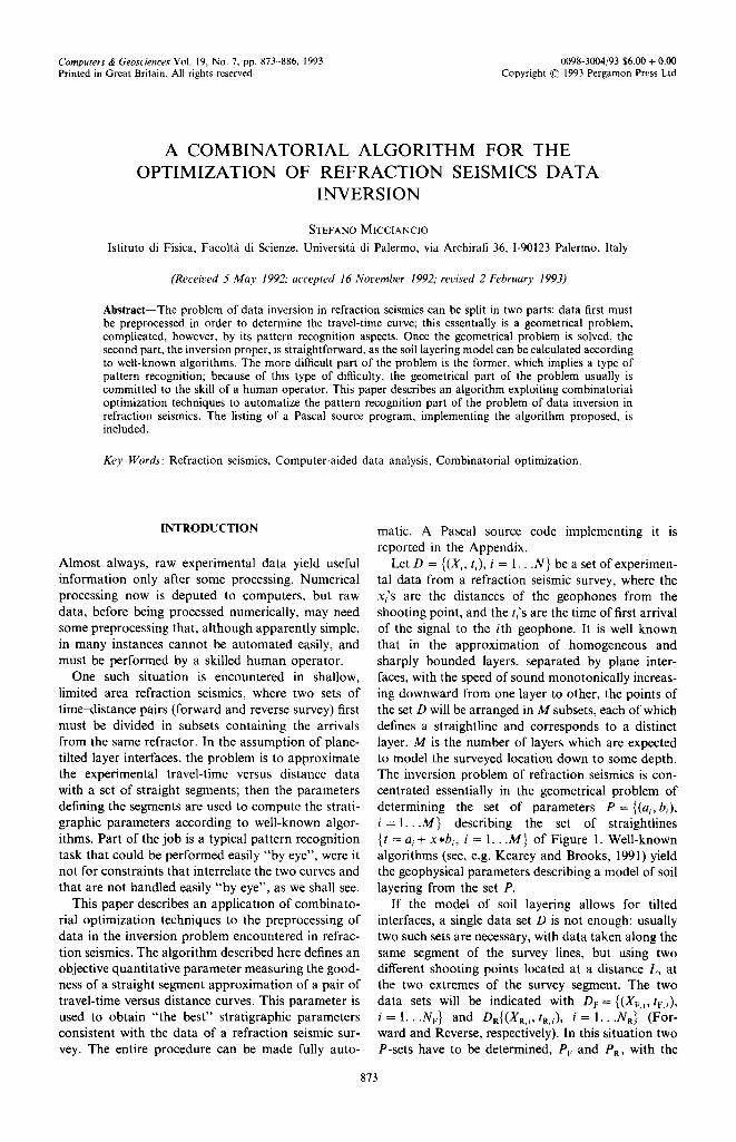
Figure 1. Plot of data in Table 1. Data of each survey (Forward = solid squares, Reverse = crosses) are grouped in subsets in order to perform fit with three-layer model. Grouping pattern shown is Ge~r, pte= {[2, 4, 5], [1, 6,4]} (see
text).
obvious change in notation. In actual surveys N F usually is equal to NR; however, for the purposes of clarity, they will be kept distinct in the following. The two sets PF and PR have the same number M of pairs, of course, but the values of their elements are not independent: in fact the relation given next must hold:
aF, iWL*bF, i=aR, i+L*bR,i, i= i . . .M. (1)
The set of Equation (1) holds if
XF,NF = XR,NR = L (2)
as is the usual situation; otherwise Equation (1) takes on a more complex form. We wish to stress that the effect of Equation (1) is to preclude the possibility of fitting separately the F-data set and the R-data set to its P-set.
The geometrical problem usually is complicated by the fact that experimental error affects the t/s and makes more difficult a clear cut allocation of the points of the D-sets to one and only one subset (or straightline). This is likely to occur, for example when an experimental point (which is affected by exper- imental error, by definition) lies near the intersection of two straightlines. In this situation only a global fit, which takes into due account the constraints imposed by Equat ion (1), is able to perform the optimal allocation of such a point.
The geometrical problem of determining the par- ameter set P from the data set D looks similar to a pattern recognition problem in the presence of noise, and in fact most current graphical (fully manual or computer assisted) procedures ultimately rely on the pattern recognition skill of the operator. In most situations the constraints imposed by Equation (i) are overlooked or neglected. In fact, they are not handled easily "by eye", even by a skilled operator.
An algorithm is described here which casts the geometrical problem as a nonlinear fit problem, taking in due account the constraints (1) and allowing a fully automatic determination of the best-fitting P-sets, thus yielding the best layering model consist-
ent with the experimental data. The algorithm can be implemented easily in a program running on a laptop computer, allowing reliable data analysis in the field.
DESCRIPTION OF THE ALGORITHM
Let the number M of layers of the model be fixed, The Nv (No) data of the D F (DR) set are grouped into M subsets (numbered from 1 to M) containing ~ , f 2 . . . . . fM (rl, r2 . . . . rM) data, respectively. More exactly: subset No. 1 of D r contains data numbered from 1 to f t , subset No. 2 contains data numbered from fl + I to fi +f2 , and so on. The fk's (rk'S) are subjected to the following constraints:
Z k f k = NF and ]~krk = N R. (3)
The set G ={{f~}, {rk}, k = 1 . . .M} is named the "grouping pattern" of the set of data {DF, Da}. Table 1 shows the sets D r and DR of a typical refraction survey with the two shooting points L = 110 m apart. The data of Table 1 are plotted in Figure I (DF: solid squares; DR: crosses), where they are grouped in subsets in order to fit a three-layer model (M = 3). The points belonging to the same subset (of the same data set) are linked by a dashed line, with a different line style for the different subsets. The grouping pattern implemented in Figure 1 is G . . . . p~e = {[2, 4, 51, [1, 6, 41}.
The kth subset of D v, as well as that of Da, define a straightline each; the two lines may be determined by any fitting algorithm: for simplicity we use the minimization of the sum of the squared residuals. However the two lines cannot be fit independently from each other, as the fit is subjected to the con- straint of Equation (1). The constrained fit may be performed, for example with the use of Lagrange's undetermined multipliers. This method is well suited to machine implementation and requires, in the pre- sent situation, the solution of a linear system with five unknowns (two parameters for each line and the Lagrange multiplier). At the end of the k th con- strained fit we get, together with the k th element of
Table 1. Typical data of refraction seismic survey. First arrival times versus position along survey line. Distance between shooting points: L = l l0m. Data provided by
Geoscience, Palermo
DF DR
i x v (m) tv (msec) XR (m) t~ (msec)
l 10 29.2 10 24.8 2 20 52,4 20 41.2 3 30 62.0 30 49.4 4 40 70.0 40 56.4 5 50 74.3 50 63.2 6 60 79.6 60 70.0 7 70 87.0 70 76.8 8 80 90.8 80 83.2 9 90 94.0 90 89.0
10 100 96.8 100 93.2 11 110 99.5 110 99.6
Optimization of refraction seismics data inversion 875
Table 2. Layering parameters of three-layers model obtained from data of Table 1 with best ten grouping patterns
Speed (m/sec) Average thickness (m) Tilt (deg) Grouping pattern Cost No. 1 No. 2 No. 3 No. 1 No. 2 No. l/No. 2 No. 2/No. 3
{[1,5,51,[1,3,71} 46.09 370 1397 2601 6.4 19.5 1.7 8.9 {[1,5,51,[1,5,51} 46.17 370 1363 2503 6.4 18.5 1.7 9.7 {[1,5,51.[1,2,81} 47.99 370 1448 2722 6.6 20.8 1.8 8.1 {[1,6,41,[1,2,8]} 48.47 370 1351 2425 6.4 17.7 1.6 10.4 {[1,5,5],[1,6,4]} 50.55 370 1205 2148 5.9 13.1 1.5 5.5 {[1,6,4],[1,3,7]} 51.15 370 1500 2845 6.7 22.0 1.8 7.2 {[1,5,5],[1,7,3]} 52.37 370 1214 2203 5.9 13.8 1.6 4.8 {[1,6,41,[1,4,61} 55.61 370 1552 2915 6.8 22.9 1.8 6.9 {[1,5,5],[1,8,21} 61.44 370 1243 2270 5.9 14.8 1.8 3.9 {[1,6,4],[1,5,5]} 61.63 370 1606 2612 7.0 21.5 1.8 11.5
the sets Pv and PR, the k th sum of squared residuals, &.
The sets Pv and PR are a property of the grouping pattern G and the sum
C = EkSk, (4)
which is named the 'cost ' of G also is a property of G. The cost allows a quantitative comparison of the goodness of the fits provided by two different group- ing patterns.
Looking at a set of real experimental data (see, e.g. Fig. 1), we may devise several reasonable grouping patterns, each of which will be characterized by its cost, that is we may define the cost C as a function of G: what we need is the value of G corresponding to the absolute minimum of C. Unfortunately G is a discrete variable and such a minimum cannot be determined by the usual analytical methods. We must resort to combinatorial optimization. The simplest and more direct way to determine the absolute mini- mum of the cost function is exhaustive search, that is to generate, by M nested loops, all the grouping patterns, which are exactly
K(N v, N R, M) = Comb(Nv - M - 1,
M - 1 ) C o m b ( N R - M - 1, M - 1) (5)
,-, 3000
"-- 2500 -
"~ 2 0 0 0 -
1500
1 0 0 0 -
~a 500 g.
o 45
O First layer + Second layer * Third layer
++ + + +
+ + +
On [] O [] O rn
L I I 5 0 5 5 6 0
Cost of the pattern
65
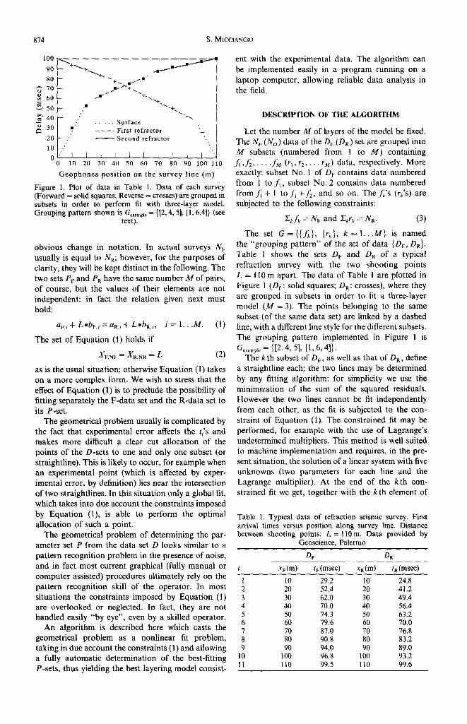
Figure 2. From data of Table 1: speed of sound (for each of three layers) versus cost of grouping pattern. Only best ten patterns are shown; arrows indicate results obtained with best one. Note that error caused by nonoptimal selection of grouping pattern is greater for lower layers.
and evaluate the corresponding costs. In Equation (5) Comb(x, y) = x !/y !(x - y)!.
The flow of a program implementing the given algorithm is:
(1) Fix M, the number of layers. (2) Generate the grouping patterns for the exper-
imental data of the sets Dv and D R. (3) For each grouping pattern:
(3.1) Calculate, for the M layers, the parameters of the two straightlines best fitting the experimental data under the constraint of Equation (1).
(3.2) Calculate the total cost of the pattern. (4) The parameters of the lines fitting the pattern
with the least cost then are worked to yield the stratigraphic parameters.
A WORKED EXAMPLE
The data of Table 1 are shown in Figure 1, where they are grouped according to the pattern Gex~mple = {[2, 4, 5], [1, 6, 4]}, which results from a fitting "by eye" with the lines shown in the figure.
The data of Table 1 have been worked with the algorithm described in the last section and
24
22 - .~ 20~+ ~a +
1 8 - 1 6 - -
1 4 - -
1 2 - -
1 o -
. ~ 6 _ n n
4 45
o First layer + Second layer
+ + +
DO [ ] [ ] o
o [ ] [ ]
I I I 5 0 55 6 0
Cost of the pattern
65
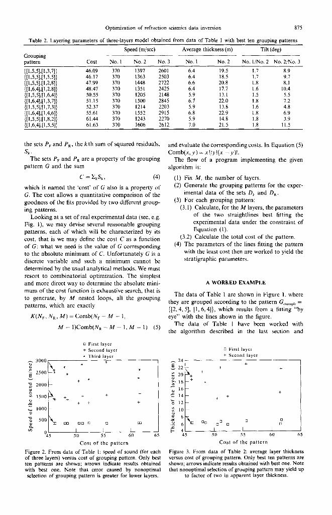
Figure 3. From data of Table 2: average layer thickness versus cost of grouping pattern. Only best ten patterns are shown; arrows indicate results obtained with best one. Note that nonoptimal selection of grouping pattern may yield up
to factor of two in apparent layer thickness.
876 S. M~CCIANCIO
~ 1 2
+ 1^/2 ̂ layer * 2^/3 ̂ layer
¢~ 10 *
; s t * .~ 7
6--
N 4 -
¢~ 23~ ÷ ++
1 - 0
~2 45
+ + + + -8-
I I I 50 55 60
Cost of the pattern 65
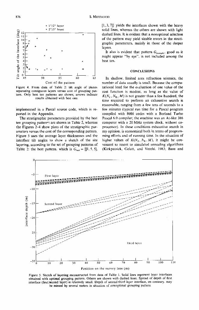
Figure 4. From data of Table 2: tilt angle of planes separating contiguous layers versus cost of grouping pat- tern. Only best ten patterns are shown; arrows indicate
results obtained with best one.
implemented in a Pascal source code, which is re- ported in the Appendix.
The stratigraphic parameters provided by the best ten grouping pat ter r ~, are shown in Table 2, whereas the Figures 2-4 show plots of the stratigraphic par- ameters versus the cost of the corresponding pattern. Figure 5 uses the average layer thicknesses and the interface tilt angles to show a sketch of the site layering, according to the set of grouping patterns of Table 2: the best pattern, which is Gb~, = {[1, 5, 5],
[1, 3, 7]} yields the interfaces shown with the heavy solid lines, whereas the others are shown with light dashed lines. It is evident that a nonoptimal selection of the pattern may yield sizable errors in the strati- graphic parameters, mainly in those of the deeper layers.
It also is evident that pattern GexamNe , good as it might appear "by eye", is not included among the best ten.
CONCLUSIONS
In shallow, limited area refraction seismics, the number of data usually is small. Because the compu- tational load for the evaluation of one value of the cost function is modest, as long as the value of K(N~., N R, M) is not greater than a few hundred, the time required to perform an exhaustive search is reasonable, ranging from a few tens of seconds to a few minutes (typical run time for a Pascal program compiled with 8086 codes with a Borland Turbo Pascal 6.0 compiler; the machine was an At-like 386 computer with a 20 MHz system clock, without co- processor). In these conditions exhaustive search in my opinion, is economical both in terms of program- ming efforts and of running time. In the situation of higher values of K(N~, N R, M), it might be con- venient to resort to simulated annealing algorithms (Kirkpatrick, Gelatt, and Vecchi, 1983: Basu and
-10
First layer
-15 ¢D
-20 i .
Second layer
-25 -- ~ ~ ~ " H'.-@;;?s / /
-30 - ~ ~ / /
i / / / /
-35 I I I 0 to 20 30
J 2 ; -
J
- 2 f f S - 2 2 2 - - J
Third layer
I I I [ I I I 40 50 60 70 80 90 100 1 1 0
Position on the survey line (m)
Figure 5. Sketch of layering reconstructed from data of Table 1. Solid lines represent layer interfaces obtained with optimal grouping pattern. Others are shown with dashed lines. Spread of depth of first interface (first/second layer) is relatively small. Depth of second/third layer interface, on contrary, may
be missed by several meters in situation of nonoptimal grouping pattern.

Optimization of refraction seismics data inversion 877
Frazer, 1990). Note, however, that simulated anneal- ing does not guarantee, in principle, the best solution in absolute, whereas the procedure described in this paper does.
The algorithm described in this paper has been implemented for plane-tilted-interface layering models, which are usual where shallow data are looked for in small area applications. In these situ- ations in fact, domes, steps, and other 'anomalies', may be present in wide area surveys, usually are not expected. The combinatorial optimization approach used, however, is of general applicability.
Acknowledgment--This work has been supported by Min- istero per la Ricerca Scientifica e Tecnologica, Fondi 60%.
REFERENCES
Basu, A., and Frazer, L. N., 1990, Rapid determination of the critical temperature in simulated annealing inversion: Science, v. 249, no. 4975, p. 1409-1412.
Kearey, P., and Brooks, M., 1991, An introduction to geophysical exploration: Blackwell, Oxford, 254 p.
Kirkpatrick, S., Gelatt, C. D. Jr., and Vecchi, M. P., 1983, Optimization by simulated annealing: Science, v. 220, no. 4598, p. 671-680.
APPENDIX
Program Listing
program dromokron;
{ Program designed and written by Stefano Micciancio Istituto di Fisica - Facolta di Scienze via Archirafi 36 - I 90123 Palermo - Italy
Pascal source code for Borland Turbo Pascal 6.0 compiler.
This program finds the best layering model (with a prescribed number of layer) consistent with data from a pair of refraction seismic surveys (Forward and Reverse, respectively).
The program asks for the number of layers of the model.
Data must be in a text (ASCII) file with the following format:
- ist line : distance between shooting points; - Data of the FORWARD survey, one point per line:
distance from shooting point, time of first arrival.
- One comment line, beginning with semicolon (;) - Data of the REVERSE survey, one point per line:
distance from shooting point, time of first arrival.
- One comment line, beginning with semicolon (;)
Output is to a text file and includes a template. )
. . . . . . . . . . . . . . . . . . . . . . . . . . . . . . . . . . . . . . . )
{ .... global constants .... ) ( .... )
const kmax = 200; nmax = 6; bestn = i0;
{
{ max. number of data per survey } { max. number of layers in the model } { max. number of best solutions stored )
) .... global data types ....
type vet5 = array[l..5] of real; mat5 = array[l..5] of vet5;
type point = record x,t : real; end;
878 S. MICCIANCIO
type pdati = ^dati; dati = record
num: integer; dat : array[l..kmax] of point; end;
type sums = record s,sx,sy,sxx,sxy,syy : real; end;
type parz = record ki,kf: integer; somme : sums; a,b : real; end;
type layer = record vel,spess,pend : real; end;
type rette = array[l..nmax] of parz; type intar = array[O..nmax] of integer; type rilev= object
pdat : pdati; nstrati : integer; ds : rette; procedure init(pd: pdati; n: integer); procedure setup(pd: pdati; cfa: intar); procedure getconf(var f: intar); procedure fit(n: integer); end;
type rt = record aa,bb,sq : real; end;
type pgfit = ~gfit; gfit = object
fwd,rev : record conf : intar; cpar : array[l..nmax] of rt; end;
bdist : real; model : array[l..nmax] of layer; kost : real; constructor init(var drt,inv: riley); function testfit: boolean; procedure modello; function testmodel: boolean; procedure print(var f: text); end;
......................................................... }
{ .... global variables .... )
var ddir,dinv : dati; drt,inv :rilev; pcfit : pgfit; lista : array[l..bestn] of pgfit; distbas : real; nnn,i : integer; f : intar; bastal,basta2 : boolean;
{ } { .... data input .... } { ) procedure pigliadati; var fdat : text;
fnam : string; ( procedure inputdati(var f: text; var dd: dati); varn : integer;
basta : boolean; rx,rt : real;
Optimization of refraction seismics data inversion 879
begin n:=0; basta:=false; while not eof(f) and not basta do
begin {$I-} read(f,rx,rt); {$I+) if ioresult=0 then begin inc(n);
with dd.dat[n] do begin x:=rx; t:=rt; end;
end else basta:=true; end;
dd.num:=n; end; {
begin
end; (
write('Data filename : '); readln(fnam); assign(fdat,fnam); reset(fdat); readln(fdat,distbas); inputdati(fdat,ddir); inputdati(fdat,dinv); close(fdat); writeln('distance between shooting points :
distbas:10:3); writeln('F : ', ddir.num, ' data; ',
'R : ', dinv.num, ' data.');
| I
. . . . . . . . . . . . . . . . . . . . . . . . .
.... results output .... ) )
procedure printall; var i,j : integer;
fn : string; f : text;
begin write('Output File Name: '); readln(fn); assign(f,fn); rewrite(f); for i:=l to bestn do
if not(lista[i]=nil) then begin writeln(f); lista[i]^.print(f); writeln(f); for j:=l to 77 do write(f,' '); writeln(f); end;
close(f); end;
. . . . . . . . . . . . . . . . . . . . . . . . . . . . . . . . . . . . . . . . . . . . . . . . . . . . . . . . . )
{ .... methods of RILEV .... ) . . . . . . . . . . . . . . . . . . . . . . . . . . . . . . )
procedure rilev.init(pd: pdati; n: integer); var cfa : intar;
i : integer; begin pdat:=pd;
nstrati:=n; cfa[0]:=pred(n); cfa[l]:=l; for i:=2 to pred(n) do cfa[i]:=cfa[pred(i)] +2; cfa[n]:=pdA.num; for i:=succ(n) to nmax do cfa[i]:=O; with ds[l] do begin ki:=l; kf:=cfa[l]; end; for i:=2 to n do with ds[i] do
begin ki:=succ(cfa[pred(i)]); kf:=cfa[i]; end; for i:=l to n do fit(i);
end; { ) procedure rilev.setup(pd: pdati; cfa: intar); var i : integer;
880 S. MICCIANCIO
begin pdat:=pd; nstrati:=succ(cfa[0]); with ds[l] do begin ki:=l; kf:=cfa[l]; end; for i:=2 to nstrati do with ds[i] do
begin ki:=succ(cfa[pred(i)]); kf:=cfa[i]; end; for i:=l to nstrati do fit(i);
end; ( procedure rilev.getconf(var f: intar); var i : integer; begin f[0]:=pred(nstrati);
for i:=l to nstrati do f[i]:=ds[i].kf; end; { procedure rilev.fit(n: integer); var i,m : integer;
zx,zy,zxx,zxy, zyy,delta : real; begin zx:=0; zy:=0; zxx:=0; zxy:=0;
end; (
zyy:=0; m:=0; if n=l then
begin for i:=ds[l].ki to ds[l].kf do begin inc(m); with pdatA.dat[i] do
begin zx:=zx+t/x; zxx:=zxx+sqr(t/x); end; end;
with ds[l] do begin a:=0; b:=zx/m; end; end
else begin for i:=ds[n].ki to ds[n].kf do with pdatA.dat[i] do
begin inc(m); zx:=zx +x; zy:=zy +t; zxx:=zxx +sqr(x); zxy:=zxy +x,t; zyy:=zyy +sqr(t); end;
with ds[n] do begin delta:=m*zxx -sqr(zx); b:=(m*zxy -zx*zy)/delta; a:=(zxx*zy -zx*zxy)/delta; end;
end; with ds[n].somme do
begin s:=m; sx:=zx; sy:=zy; sxx:=zxx; sxy:=zxy; syy:=zyy; end;
.... methods of GFIT ....
constructor gfit.init(var drt,inv: rilev); var vx,vb : vet5;
ma : mat5; sd,si : sums; i,j,k,nn : integer; ccf : intar; { procedure linear_solve(A: mat5; var y: vet5; b: vet5); { solves the linear system Ay=b ) ( procedure adapted from 'Numerical Recipes'
by Press, Flannery, Teukolsky and Vetterling, (Cambridge University Press, 1986. )
CONST tiny = 1.0e-20; matdim = 5;
Optimization of refraction seismics data inversion 881
VAR imax,i,j,k, ip,ii : integer; big,dum,x : real; sum : double; w : vet5; permut : array[l..matdim] of integer;
begin for i:=l to matdim do begin big:=0; for j:=l to matdim do
begin x:=abs(a[i,j]); if x>big then big:=x; end;
if (big=0) then begin writeln('singular matrix '); halt; end;
vv[i]:=i/big; end;
for j:=l to matdim do begin if (j>l) then
for i:=l to pred(j) do begin sum :=a[i,j]; if (i>l) then
begin for k:=l to pred(i) do sum:=sum -a[i,k]*a[k,j];
a[i,j]:=sum; end;
end; big:=0; for i:=j to matdim do
begin sum:=a[i,j]; if (j>l) then
begin for k:=l to pred(j) do sum:=sum -a[i,k]*a[k,j];
a[i,j]:=sum; end;
dum:=vv[i]*abs(sum); if (dum>big) then
begin big:=dum; imax:=i end; end;
if not(j=imax) then begin for k:=l to matdim do
begin dum:=a[j,k]; a[j,k]:=a[imax,k]; a[imax,k]:=dum; end;
vv[imax]:=vv[j]; end;
permut[j]:=imax; if not(j=matdim) then
begin if (a[j,j]=0) then a[j,j]:=tiny; dum:=i/a[j,j]; for i:=succ(j) to matdim do
a[i,j]:=a[i,j]*dum; end;
end; if (a[matdim,matdim]=0) then
a[matdim,matdim]:=tiny;
ii:=0; for i:=l to matdim do
begin ip:=permut[i]; sum:=b[ip]; b[ip]:=b[i]; if not(ii=0) then
for j:=ii to pred(i) do sum:=sum-a[i,j]*b[j]
else if not(sum=0) then ii:=i; b[i]:=sum; end;
882 S. MICCIANCIO
for i:=matdim downto 1 do begin sum:=b[i]; if (i<matdim) then
for j:=succ(i) to matdim do sum:=sum-a[i,j]*b[j];
b[i]:=sum/a[i,i]; end;
end; (
y:=b;
begin nn:=drt.nstrati; bdist:=distbas; drt.getconf(ccf); fwd.conf:=ccf; inv.getconf(ccf); rev.conf:=ccf; i:=l; sd:=drt.ds[i].somme; si:=inv.ds[i].somme; with fwd.cpar[i] do
begin aa:=0; bb:=(sd.sx +si.sx)/(sd.s +si.s); sq:=0; for k:=drt.ds[i].ki to drt.ds[i].kf do
sq:=sq +sqr(aa +bb*drt.pdat^.dat[k].x -drt.pdatA.dat[k].t );
end; with rev.cpar[i] do
begin aa:=0; bb:=(sd.sx +si.sx)/(sd.s +si.s); sq:=0; for k:=inv.ds[i].ki to inv.ds[i].kf do
sq:=sq +sqr(aa +bb*inv.pdat^.dat[k].x -inv.pdatA.dat[k].t );
end; for i:=2 to nn do
begin sd:=drt.ds[i].somme; si:=inv.ds[i].somme; for j:=l to 5 do for k:=l to 5 do ma[j,k]:=0; ma[l,l]:=sd.s; ma[l,2]:=sd.sx; ma[l,5]:=i/2; vb[l]:=sd.sy; ma[2,1]:=sd.sx; ma[2,2]:=sd.sxx; ma[2,5]:=distbas/2; vb[2]:=sd.sxy; ma[3,3]:=si.s; ma[3,4]:=si.sx; ma[3,5]:=-i/2; vb[3]:=si.sy; ma[4,3]:=si.sx; ma[4,4]:=si.sxx; ma[4,5]:=-distbas/2; vb[4]:=si.sxy; ma[5,1]:=l; ma[5,2]:=distbas; ma[5,3]:=-l; ma[5,4]:=-distbas; vb[5]:=0; linear solve(ma,vx,vb); with fwd.cpar[i] do
begin aa:=vx[l]; bb:=vx[2]; sq:=0; for k:=drt.ds[i].ki to drt.ds[i].kf do
sq:= sq +sqr(aa +bb*drt.pdat^.dat[k].x -drt.pdat^.dat[k].t);
end;
Optimization of refraction seismics data inversion 883
end; (
with
end; kost:=O; for i:=l
kost:
rev.cpar[i] do begin aa:=vx[3]; bb:=vx[4]; sq:=O; for k:=inv.ds[i].ki to inv.ds[i].kf do
sq:= sq +sqr(aa +bb*inv.pdat^.dat[k].x -inv.pdat^.dat[k].t);
end;
to nn do =kost +fwd.cpar[i].sq +rev.cpar[i].sq;
function gfit.testfit: boolean; { Used to reject the grouping pattern if the sound speed of any layer is negative. (It might occur in case of large random experimental errors.) )
var ok : boolean; i : integer;
begin ok:=true; with fwd do
for i:=l to succ(conf[O]) do ok:=ok and (cpar[i].bb>O);
with rev do for i:=l to succ(conf[O]) do
ok:=ok and (cpar[i].bb>O); testfit:=ok;
end; . . . . . . .
function gfit.testmodel: boolean; { Used to reject the grouping pattern if any layer thickness is negative. (It might occur in case of large random experimental errors.) )
var ok : boolean; i : integer;
begin ok:=true; for i:=2 to succ(fwd.conf[O]) do
ok:=ok and (model[i].spess >0); testmodel:=ok;
end; ( procedure gfit.modello; var hf,kf,dkf,tf,dtf,pf,rf,bbf,lf,qf : real;
hr,kr,dkr,tr,dtr,pr,rr,bbr, lr,qr : real; gc,vc,gs,vs,th,dtg,cgct,hh,ddm : real; n,i : integer;
begin hf:=O; kf:=O; dkf:=O; tf:=O; dtf:=O; hr:=O; kr:=O; dkr:=O; tr:=O; dtr:=O; gc:=O; vc:=O; gs:=O; th:=O; vc:=i/fwd.cpar[l].bb; with model[l] do
begin vel:=vc; pend:=O; spess:=O; end; n:=succ(fwd.conf[O]); ddm:=bdist/2; i:=2; while i<=n do
begin bbf:=vc*(fwd.cpar[i].bb -dtf)/(l -dkf); bbr:--vc*(rev.cpar[i].bb -dtr)/(l -dkr); if:=bbf*cos(gc); ir:=bbr*cos(gc);
if (abs(if)>l) or (abs(ir)>l) then begin model[i].vel:=-l; model[i].spess:=-l; i:=succ(n); end
else begin if:=arctan(if/sqrt(l+sqr(if))); ir:=arctan(ir/sqrt(l+sqr(ir)));
884 S. MICCIANCIO
end; (
end;
th:=(if +ir)/2; gs:=(ir -if)/2 -gc; hh:=((hf +kr)*bbr +(hr +kf)*bbf
+vc*(fwd.cpar[i].aa -tf +rev.cpar[i].aa -tr))
/(4*cos(th)*cos(gs)) ; vs:=vc/sin(th); with model[i] do
begin vel:=vs; pend:=gs; spess:=hh; end;
dtg:=sin(gs)/cos(gs) -sin(gc)/cos(gc); cgct:=cos(gs)/cos(th); qf:=(l-dkf)*dtg*cgct/vc; qr:=(l-dkr)*dtg*cgct/vc; dtf:=dtf -qf; dtr:=dtr +qr; dkf:=dkf -qf*sin(th-gs); dkr:=dkr +qr*sin(th+gs); pf:=(hh+dtg*(ddm-hf))*cgct; pr:=(hh-dtg*(ddm-hr))*cgct; rf:=(hh+dtg*(ddm+kf))*cgct; rr:=(hh-dtg*(ddm+kr))*cgct; hf:=hf +pf*sin(th +gs); hr:=hr +pr*sin(th -gs); kf:=kf +rf*sin(th -gs); kr:=kr +rr*sin(th +gs); tf:=tf +(pf +rf)/vc; tr:=tr +(pr +rr)/vc; gc:=gs; vc:=vs; inc(i); end;
procedure gfit.print(var f: text); var j,ns : integer;
gp : string;
function getpat(cc: intar): string; var ps,ss : string;
j,kk : integer; begin ps:='[';
for j:=l to ns do begin if (j=l) then kk:=succ(cc[j]) else kk:=cc[j] -cc[pred(j)]; str(kk:2,ss); ps:=ps + ss; if j<ns then ps:=ps + ','; end;
ps:=ps +']'; getpat:=ps;
end;
begin ns:=succ(fwd.conf[O]); gp:='{'+getpat(fwd.conf)+','+getpat(rev.conf)+')'; writeln(f,' grouping pattern = ',gp); writeln(f,'cost of the pattern = ',kost:12:6); writeln(f); writeln(f,
' I ... forward data ..... I', ' ... reverse data ..... I', ' speed tilt thick');
writeln(f, ' n I intercept slope I', ' intercept slope I', ' [m/s] [°] [m] ');
for j:=l to ns do begin
Optimization of refraction seismics data inversion 885
write(f,j:2,' I', fwd.cpar[j].aa:ll:6,fwd.cpar[j].bb:ll:6,' ', rev.cpar[j].aa:ll:6,rev.cpar[j].bb:ll:6,' ', 1000*model[j].vel:7:0, 180*model[j].pend/pi:7:l);
if j<ns then writeln(f,model[succ(j)].spess:8:l) else writeln(f); end;
end; (--- )
{ .... flow management .... ) ( }
procedure insert(pp: pgfit); { Sorts the grouping patterns in order of decreasing cost.} var i,k : integer;
basta : boolean; begin if (lista[l]=nil) then lista[l]:=pp
else begin i:=l; basta:=false; repeat if pp^.kost<=lista[i]^.kost then
begin for k:=bestn downto succ(i) do lista[k]:=lista[pred(k)];
lista[i]:=pp; basta:=true; end;
inc(i); (i>bestn) or basta; until
end; end; ( .... }
function nextconf(var x: intar): boolean; ( Generates all possible grouping patterns. var i,j,ns,nd : integer; begin ns:=succ(x[0]);
nd:=x[ns]; i:=pred(ns); while (x[i] =(nd -2*(ns -i))) and (i>0) if (i=0) then nextconf:=false else if x[l]<pred(nd div ns) then
begin inc(x[i]); for j:=succ(i) to pred(ns) do
x[j]:=x[pred(j)] +2; nextconf:=true; end
else nextconf:=false;
do dec (i) ;
end; { .... }
{ ............ main ............ ) . . . . . . . . . . . . . . . . . . . . . . . . . . . . . . . . . . . . . . . . . . . . . . -- . . . . . . . . . . }
begin for i:=l to bestn do lista[i] :=nil; pigliadati; write('number of layers in the model: '); readln(nnn); drt.init(@ddir,nnn); basta2:=false; repeat inv.init(@dinv,nnn);
bastal:=false; repeat new(pcfit); pcfit^.init(drt,inv);
if pcfit^.testfit then begin pcfitA.modello; if pcfit*.testmodel then insert(pcfit) else dispose(pcfit); end
else dispose(pcfit); inv.getconf(f); if nextconf(f) then inv.setup(@dinv,f) else bastal:=true;
until bastal;

886 S. MICCIANCIO
end.
drt.getconf(f); if nextconf(f) then drt.setup(@ddir,f) else basta2:=true;
until basta2; printall; for i:=l to bestn do
if not(lista[i]=nil) then dispose(lista[i]);