Embed Size (px)
Citation preview

Research ArticleA Combined Localization Algorithm forWireless Sensor Networks
Xiaogang Qi12 Xiaoke Liu 12 and Lifang Liu3
1School of Mathematics and Statistics Xidian University Xirsquoan 710071 China2State Key Laboratory of Satellite Navigation System and Equipment Technology Shijiazhuang 050000 China3School of Computer Science and Technology Xidian University Xirsquoan 710071 China
Correspondence should be addressed to Xiaoke Liu xiaokeliu1163com
Received 18 December 2017 Revised 10 May 2018 Accepted 12 June 2018 Published 3 July 2018
Academic Editor Salvatore Alfonzetti
Copyright copy 2018 Xiaogang Qi et al This is an open access article distributed under the Creative Commons Attribution Licensewhich permits unrestricted use distribution and reproduction in any medium provided the original work is properly cited
Wireless sensor networks (WSNs) are widely used in various fields to monitor and track various targets by gathering informationsuch as vehicle tracking and environment and health monitoring The information gathered by the sensor nodes becomesmeaningful only if it is known where it was collected from Considering that multilateral algorithm andMDS algorithm can locatethe position of each node we proposed a localization algorithm combining themerits of these two approaches which is calledMA-MDS to reduce the accumulation of errors in the process of multilateral positioning algorithm and improve the nodesrsquo positioningaccuracy in WSNs It works in more robust fashion for noise sparse networks even with less number of anchor nodes In the MDSpositioning phase of this algorithm the Prussian Analysis algorithm is used to obtain more accurate coordinate transformationThrough extensive simulations and the repeatable experiments under diverse representative networks it can be confirmed that theproposed algorithm is more accurate and more efficient than the state-of-the-art algorithms
1 Introduction
Wireless sensor networks are composed of a large number ofsensor nodes with sensing computing and wireless commu-nication capabilities They are widely used in military recon-naissance environmentalmonitoring smart home and otherfields Interestingly the location service ofWSN is a guaranteeof important services such as information collection targettracking and information management Only by obtainingthe location of the sensor node corresponding to the collectedinformationwill the datamake senseTherefore determiningthe location information of sensor nodes becomes particu-larly important in WSNs Global Navigation Satellite systems(INS) and Global Positioning System (GPS) have been widelyemployed for localization but it is unpractical and costly tointegrate a GPS receiver in each sensor of an entire large-scalesensor network A large number of localization algorithmsthus are proposed
Existing localization algorithms mainly fall into twostrategies range-free and range-based approaches accordingto whether the distance between nodes is to be measured
before positioning Range-based algorithms include trilateralalgorithm [1] multilateral algorithm [2] DEP algorithm [3]etc Specifically the multilateral algorithm [2] possessing ofhigh positioning accuracy is a commonly used algorithmamong them An equation can be constructed by usingthe distance between the anchor nodes and the unknownnodes and then the solution can be worked out via theleast square method in the algorithm The disadvantageof this method is that the selection of the anchor nodeserial number will have some influence on the positioningaccuracy in the process of constructing the equation Range-free algorithms comprise centroid localization algorithm [4]APIT (Approximate Point-in-Triangulation Test) algorithm[5] DV-Hop (Distance Vector-Hop) algorithm [6] etc Thecentroid location algorithm [4] is very simple and conve-nient but entirely based on network topology which canbe influenced by communication range of nodes The rangemay be disturbed by various factors in practice bringingabout a relatively large error By determining the locationrelationship between the unknown node and the neighboranchor nodes the APIT algorithm [5] keeps shrinking
HindawiMathematical Problems in EngineeringVolume 2018 Article ID 4648109 10 pageshttpsdoiorg10115520184648109
2 Mathematical Problems in Engineering
and covering the unknown area ultimately approachingthe unknown node The APIT algorithm relies on highlyconnectivity of nodes so this algorithm is not suitable forsparse networks The DV-Hop algorithm [6] is one of thepopular hop-count localization methods which obtains theinformation of each anchor nodemainly through the distancevector routing protocol However with the increase of thehop count between the anchor node and the unknown nodethe gradually accumulating measured distance leads to thepoor positioning accuracy of unknown nodes Moreover[7] compares the performance of APIT algorithm with DV-Hop algorithm in detail and the results show that theperformance of DV-Hop algorithm is much better than ofthe APIT algorithm no matter how the number of anchornodes changesThe localization algorithm based onMDS [8ndash10] can be considered as the range-based algorithm as well asthe range-free algorithm and this paper mainly considers itas range-based algorithm More narrowly the WSNs can beregarded as a weighted undirected graph with the weight isthe distance between two adjacent nodes Distance matrix asthe only input of MDS algorithm derives from the shortestpath calculated by Floyd algorithm between any two nodesIt is well known that the accuracy of the MDS algorithmis closely related to the hops between nodes The largerthe hops the larger the error of replacing the real distancewith the shortest path distance which eventually lead topoor positioning accuracy of theMDS algorithm Comparingrange-based algorithmwith range-free algorithm the formerhas higher hardware cost but has high localization accuracyIn the application scenarioswith high accuracy requirementsrange-based algorithms are generally adopted
Based on the range-based localization algorithm andthe range-free localization algorithm some researchers haveproposed the idea of combining the heuristic optimizationalgorithm with the WSN node localization technology Theprinciple of this idea is to construct the optimal position-ing model by obtaining the distance information betweennodes or the connected topological relations and use theheuristic optimization algorithm to calculate the optimalsolution by iterating the optimal positioning model Sofar many optimization algorithms have been used in therealm of heuristic optimization algorithms such as Simu-lated Annealing (SA) [11] Artificial Fish Swarm Algorithm(AFSA) [12] Flower Pollination Algorithm (cFPA) [13] andParticle SwarmOptimization (PSO) [14] Carrying out a greatnumber of simulation experiments on the above heuristicalgorithmwe intuitively discover that the heuristic algorithmis too computationally expensive and time-consuming for thecentralized localization optimization to apply in the real scenelocalization In addition a universal weakness of heuristicalgorithms is that they are overly dependent on the initialparameters Improper selection of the initial parameters maycause the localization algorithm to be paralyzed
Ultrawide Band (UWB) technology first appeared in1960 radar applications has now developed into an emergingtechnologies which sets wireless data communications andreal-time sensing as a whole Differing from the traditionalcommunication technologies UWB technology is a pulsedradio technology which transmits data through extremely
short nanosecond pulses replacing carrier signals betweentransceivers According to the definition and characteristicsof the signal UWB technology has the advantages of largebandwidth fast transmission low transmission power highmultipath resolution and strong antifading UWB rangingtechniques commonly used today can be categorized intoTime of Arrival (TOA) Time Difference of Arrival (TDOA)Angle of Arrival (AOA) and Received Signal Strength Indi-cation (RSSI) TOA technique requires precise clock synchro-nization technique so the hardware requirements are higherTheprinciple of TDOA is to use the difference of transmissionspeed by wireless signal or ultrasonic signal to measurethe distance between nodes It has higher ranging accuracybut needs to be equipped with ultrasonic launcher fornodes which increases the hardware cost AOA algorithmsneed antenna arrays to extract angle information RSSI is atechnique for measuring the distance between nodes basedon the power loss of a wireless signal during transmissionSince the inherent wireless communication chip in the nodehas the ability to calculate and transmit signals RSSI doesnot require additional hardware In addition the accuracy ofthe localization algorithm based on RSSI has obvious meritscompared with that of range-free algorithm so this paperselects RSSI ranging technology for measuring the distancebetween nodes
In large-scale sensor networks with anchor nodes dis-tributed on the edge due to the limitation of communicationrange the location of all unknown nodes could not beobtained by one-time multilateral algorithm and they mustbe hierarchically positioned firstly finding all unknownnodes adjacent to at least three anchor nodes called 1-levelnodesThen the multilateral algorithms are used to calculatethe estimated position of the 1-level nodes Further the 1-level nodes as new anchor nodes join into the anchor nodeset At this point the 1-level nodes location ends Similarto the steps of positioning the 1-level nodes nodes from 2-level to n-level can be located by the multilateral algorithmuntil all the unknown nodes have obtained the geographicalposition As can be seen from the above steps themultilateralalgorithmwill produce the cumulative error the more nodesrsquolevel the greater the cumulative error the poorer positioningaccuracy In order to prevent overaccumulation of cumulativeerror this paper presents a combined algorithm (MA-MDS)which uses theMDS algorithm to calculate the location of theremaining unknown nodes after positioning a specific levelof nodes (such as six-level nodes) location by the multilateralalgorithm
We will examine the performance of MA-MDS onnetworks of 100 to 200 nodes with node locations eitherchosen randomly or deployed according to a rough grid andcompared the positioning error of the MA-MDS algorithmwith other representative algorithms It is worth stating thatthe anchor nodes in this article are only distributed on theedge of the node deployment area to cater to some specialapplication scenarios
The rest of paper is organized as follows In Section 2 wediscuss related work Section 3 describes show the MA-MDSalgorithm Computer simulation results and experimentanalysis are shown in Sections 4 and 5
Mathematical Problems in Engineering 3
2 Problem Description
21 Problem Formulation Consider a WSN with 119873 wire-less nodes labeled 1 2 119873 in 2-dimensional space Thenumber of anchors whose locations are all known already is119872(119872 lt 119873) so there are119873minus119872 unknown nodes that shouldbe localized in this problem By usingRSSI signal propagationmodel we can estimates the distance from one node to itsneighbors Denote the distance measured between nodes 119894and 119895 as 119889119894119895 Let 119883 = 119909119894119873119894=1 119909119894 = [119909119894 119910119894] isin R represents thereal coordinates of all nodes and119860 = 119909119894119872119894=1 represents the setof anchor nodesrsquo coordinates Note that anchor nodes mustbe distributed on the edge of the node deployment area
22 Error in Localization Problem Consider a WSN withwireless sensor nodes which include 119872 anchors and 119873 minus119872unknown nodes and define the average location error inWSN as follows
Definition 1 Average Localization Error is
119864119903119903119900119903119860 = sum119873minus119872119894=1 radic(119909119894 minus 119909119894)2 + (119910119894 minus 119910119894)2(119877 lowast (119873 minus119872)) (1)
where119877 is the communication radius of the node in network
23 RSSI Signal Propagation Model An important featureof wireless signal transmission is that the strength of signalattenuates with the increase of distanceThemost widely usedsimulation model to generate RSSI samples as a function ofdistance in Radio Frequency (RF) channels is the log-normalshadowing model [15]119875119877 (119889) = 119875119879 minus 119875119871 (1198890) minus 10120578 lg( 1198891198890 + 119883120590) (2)
where 119875119877 is the received signal power 119875119879 is the transmitpower and 119875119871(1198890) is the path loss for a reference distanceof 1198890 120578 is the path loss exponent and 119883120590 is a zero-meanGaussian noise with a standard deviation 120590 which means119883120590 sim 119873(0 1205902) All powers are in 119889119861 and all distances are inmeters Moreover in this model we assume there is notobstruction like walls between nodes
3 Localization Algorithm
This section mainly introduces MA-MDS localization frame-work described MDS algorithm and multilateral algorithmin detail As mentioned in Section 1 MA-MDS is an algo-rithm combining the advantages of the multilateral algo-rithm and the MDS algorithm Multilateral algorithms areprone to produce large errors of high-level nodes as the effectof cumulative error and the reverse is true for the low-levelnodes Therefore MDS algorithm is used to positioning thehigh-level nodes with larger errors to obtain more accurateresults The detailed process of the MA-MDS algorithm is asfollows Primarily themultilateral algorithm is used to obtainthe estimated coordinates of the nodes from 1-level to k-level
nodes as set B and each node in B can be regarded as anew anchor node namely 119860 = 119860 cup 119861 Next we have to getthe distance matrix that the MDS algorithm needs to inputThe solution is to get the weighted shortest path distance byusing Floyd algorithm Finally running the MDS algorithmto get the relative map and then the Procrustes analysis (PA)algorithm [16 17] is referenced to convert the relative mapinto an absolute map (estimated node location) It should benoted that at this moment the anchor nodes are union of allestimated nodes calculated by the multilateral algorithm andthe original anchor nodesThe detailed flow of the MA-MDSalgorithm is shown in Algorithm 1
There is a problem pressing to be solved is how to deter-mine the threshold k so that when 119894 gt 119896 the i-level nodesare called the high-level nodes and are instead called thelow-level nodes when 119894 le 119896 is satisfied Obviously since thedistribution of nodes varies under different application sce-narios the selection of kmay change In the simulation exper-iment of this paper the selection of k will be described indetail in Section 4
The detailed introduction and analysis of multilateralalgorithm and MDS algorithm are as follows
31 The MDS Algorithm MDS is a set of mathematicaltechniques which have their origins in psychometrics andpsychophysics MDS has been applied in many fields suchas computational chemistry machine analysis and targetlocalization When used for localization MDS takes fulladvantage of connectivity or distance information betweenknown and unknown nodes
Use119883 = [119909119894 119910119894]119873times2 to denote the true locations of the setof119873wireless nodes in 2-dimensional space 119889119894119895(119883) representsthe Euclidean distance between the nodes 119894 and 119895119889119894119895 (119883) = radic((119909119894 minus 119909119895)2 + (119910119894 minus 119910119895)2) (3)
Let119867 = 119883 sdot 119883119879 and we can get[119889119894119895 (119883)]2 = 1199092119894 + 1199102119894 + 1199092119895 + 1199102119895 minus 2 (119909119894119909119895 + 119910119894119910119895)= 119867119894119894 + 119867119895119895 minus 2119867119894119895 (4)
We can get (6) after applying double center to119883
119873sum119894=1
119867119894119895 = 0 (5)
Then 1119873 119873sum119894=1
1198892119894119895 = 1119873 119873sum119894=1
119867119894119894 + 119867119895119895 (6)1119873 119873sum119895=1
1198892119894119895 = 1119873 119873sum119895=1
119867119895119895 + 119867119894119894 (7)
11198732 119873sum119894=1
119873sum119895=1
1198892119894119895 = 2119873 119873sum119894=1
119867119894119894 (8)
4 Mathematical Problems in Engineering
Inputs(i) A the set of anchor nodes locations(ii) k threshold(iii) 119861119894 the estimated coordinates of i-level nodes
Outputs(i) 119883119873times2 the estimated coordinates of all nodes in the entire WSNs
Step 1 Low-level nodes positioningFor i=1 to k do(i) Find the set of i-level nodes(ii) Running the multilateral algorithm to obtain the estimated coordinates of the i-level nodes 119861119894(iii) Refresh the set of anchor nodes coordinates 119860 fl 119860 cup 119861119894End for
Step 2 High-level nodes positioning(i) Get the weighted shortest path distance matrix by using Floyd algorithm119863119873times119873(ii) Running MDS algorithm get relative coordinates for all nodes in WSNs 119877119873times2
the relative coordinates of anchor nodes are 119860(iii) Transform relative coordinates to absolute coordinates by PA algorithm
get finally estimated coordinates of all nodes119883119873times2Step 3 Calculation error
(i) Calculate average localization error by Eq (1)
Algorithm 1 The MA-MDS algorithm
A1 (x1y1)
A2 (x2y2)
A3 (x3y3) A4 (x4y4)
A5 (x5y5)
Al (xlyl)
B (xy)
Figure 1 The schematic of the multilateral algorithm
Further119867119894119895 = 12 ( 1119873 119873sum119895=1
1198892119894119895 + 1119873 119873sum119894=1
1198892119894119895 minus 1198892119894119895 minus 11198732 119873sum119894=1
119873sum119895=1
1198892119894119895) (9)
Calculate the Singular Value Decomposition (SVD) of119867119867 = 119880119881119880119879 (10)
where 119880 = (1199061 1199062 119906119873) 119881 = diag(V1 V2 V119873)Let 119883 = 11988011988112 the localization scenes is 2-dimensional
space so get the first two rows of119883 which is relative locationof nodes We need eventually to get the absolute position ofnodes which can be achieved from the rigid transformation(rotation scaling and translation) This transformation canbe achieved using Procrustes analysis (PA) algorithm
32 The Multilateral Algorithm Figure 1 shows the anchornodes1198601 119860 119897 (119897 lt 119872)with their coordinates (1199091 1199101)
(119909119897 119910119897) and the unknown node 119861(119909 119910) From them thedistance between anchors and unknownnodes can beworkedout Consider the distance between anchor nodes and theunknown node as 1198891 1198892 119889119897
According to the Pythagoras theorem the distance equa-tion is (119909 minus 1199091)2 + (119910 minus 1199101)2 = 11988921(119909 minus 1199092)2 + (119910 minus 1199102)2 = 11988922(119909 minus 119909119897)2 + (119910 minus 119910119897)2 = 1198892119897
(11)
By dealing with (11) we have2 (1199091 minus 119909119897) 119909 + 2 (1199101 minus 119910119897) 119910 = 11990921 minus 1199092119897 + 11991021 minus 1199102119897 minus 11988921+ 11988921198972 (1199092 minus 119909119897) 119909 + 2 (1199102 minus 119910119897) 119910 = 11990922 minus 1199092119897 + 11991022 minus 1199102119897 minus 11988922+ 1198892119897 2 (119909119897minus1 minus 119909119897) 119909 + 2 (119910119897minus1 minus 119910119897) 119910 = 1199092119897minus1 minus 1199092119897 + 1199102119897minus1minus 1199102119897 minus 1198892119897minus1 + 1198892119897(12)
Mathematical Problems in Engineering 5
Equation (12) can be expressed in matrix form
( 2(1199091 minus 119909119897) 2 (1199101 minus 119910119897)2 (1199092 minus 119909119897)2 (119909119897minus1 minus 119909119897)2 (1199102 minus 119910119897)2 (119910119897minus1 minus 119910119897) )(119909119910)
= ( 11988711198872119887119897minus1)(13)
Let
A = ( 2(1199091 minus 119909119897) 2 (1199101 minus 119910119897)2 (1199092 minus 119909119897)2 (119909119897minus1 minus 119909119897)2 (1199102 minus 119910119897)2 (119910119897minus1 minus 119910119897) )
X = (119909119910) b = ( 11988711198872119887119897minus1)
(14)
Equation (13) can be written as AX = bThen the least squares solution can be calculated as1006704X = (A119879A)minus1 A119879b (15)
Thus the estimated coordinates of unknown nodes areobtained
33 Procrustes Analysis (PA)Algorithm TheProcrustes prob-lem is to get the matrix Q which satisfies AQ as close aspossible to B there A and B are given
We begin by defining the set OS119905(119901 119896) of orthogonalStiefel matrices
OS (119901 119896) = 119876 119876 isin R119901times119896 119876119879119876 = 119868119896times119896 (16)
Let 119860 isin R119898times119896 and 119861 isin R119898times119901 (119898 ge 119901 ge 119896)Let 119860119865 = (119905119903119886119888119890(119860119879119860))12 denote the standard Frobe-
nius norm in R119898times119896The Procrustes problem for orthogonal Stiefel matrices
can be expressed in formula119891 (119876) = min119876
119860119876 minus 1198612119865 (17)
where 119876 isin OS(119901 119896)
When 119901 = 119896 (17) is called the equilibrium Procrustesproblem
This research tries to use the Procrustes analysis toconvert the relative coordinates to absolute coordinates Use119866119872times2 to denote the true locations of the set of 119872 anchornodes and 119884119872times2 to denote the estimated locations of the setof 119872 anchor nodes The purpose is to find the transformedcoordinate matrix 1198841015840119872times2 so that the mean square errorof 1198841015840119872times2 and 119866119872times2 is minimized119884lowast = 119904119884119879 + 119890119905119879 119890 = (1 1 1)119879119872times1 (18)
In the above formula 119878 is the scaling factor 119905 is thecoordinate translation vector and 119879 is the rotation mirrormatrix
Through the above analysis the Procrustes problem is
min 119871 (119904 119905 119879)= 119905119903 [119866 minus (119904119884119879 + 119890119905119879)]119879 [119866 minus (119904119884119879 + 119890119905119879)] (19)
In order to weaken the correlation between the transfor-mation parameters and the rotation parameters centralizedprocessing of X and Y is119869 = 119868 minus 1119872119890 lowast 1198901198791198661015840 = 1198691198661198841015840 = 119869119884 (20)
Then formula (20) can be simplified as
min119871 (119904 119879) = 119905119903 [1198661015840 minus 1199041198841015840119879]119879 [1198661015840 minus 1199041198841015840119879] (21)
The process of solving the minimum value by Lagrangefunction method is as follows119891 = 119905119903 [1198661015840 minus 1199041198841015840119879]119879 [1198661015840 minus 1199041198841015840119879]minus 119905119903 [120582 (119879119879119879 minus 119868)] (22)
120597119891120597119879 = minus2119904 (1198841015840)1198791198661015840 + 2119904 (1198841015840)119879 1198841015840119879 minus 119879 (120582 + 120582119879) (23)
Let 119876 = (1198841015840)1198791198661015840 119875 = (1198841015840)1198791198841015840 and ℎ = (120582 + 120582119879)2 then120597119891120597119879 = minus2119904119876 + 2119904119875119879 minus 2119879ℎ = 0ℎ = minus119904119879119879119876 + 119904119879119879119875119879 (24)
In formula (24) since both ℎ and 119904119879119879119875119879 are symmetricmatrices 119879119879119876 is symmetric matrices119876119876119879 = 119879119876119879119879119879119879119876119879119879 = 119879119876119879119876119879119879 (25)
The Singular Value Decomposition of 119876 is119876 = 119880Σ119881119879 Σ = diag (1205901 120590119903) (26)
6 Mathematical Problems in Engineering
Table 1 Parameters used for grid placement
Variable ValueMap size 200119898 times 200119898Sensor nodes 121Anchor nodes 20Radio range 30m
We have119876119876119879 = 119880Σ119881119879119881Σ119880119879 = 119880Σ2119880119879119876119876119879 = 119879119876119879119876119879119879 = 119879119881Σ2119881119879119879119879 (27)120597119891120597119904 = minus2119905119903 (1198661015840 minus 1199041198841015840119879) (1198841015840119879)119879= minus2119905119903 (11988410158401198791198661015840) + 2119904119905119903 (1198841015840 (1198841015840)119879) = 0 (28)
Solving formulas (27) and (28) we can get119879 = 119880119881119879119904 = 119905119903 (1198661015840)119879 1198841015840119879119905119903 (1198841015840)119879 1198841015840 = 119905119903 (119866119879119869119884119879)119905119903 (119884119879119869119884) 119905 = 1119872 (119866 minus 119904119884119879)119879 119890
(29)
After the various parameters are obtained by formula(29) all the coordinates in the relative map can be convertedto absolute coordinates
4 Complexity and Simulation Results Analysis
41 Time Complexity Analysis Assume that the total numberof nodes in the network is 119873 and the number of anchornodes is 119872 The original classic MDS algorithm uses acentralized calculation method The time complexity of theshortest path distance between nodes calculated by Floydalgorithm is 119874(1198733) and that of MDS algorithm is 119874(1198733)The time complexity of the multilateral algorithm is 119874(1198732)For the heuristic optimization algorithms we assume that themaximum number of iterations is119898 the population numberis 119899 the number of try times is 119871 and the number of decisionvariables that is the dimension of space is 119863 The timecomplexity of the algorithm is 119874(119873 lowast 119899 lowast 119898 lowast 119871 lowast 119863) 119899 isthe number of fishes and pollen in the AFSA [12] and cFPA[13] respectively Setting the simulation parameters of AFSAalgorithm as 119899 = 119898 = 119871 = 12119873 the time complexity ofthis algorithm is 119874(1198734) while the time complexity of MA-MDS algorithm is 119874(1198733) Obviously the time complexity ofthe MA-MDS algorithm is lower than that of the heuristicalgorithm
42 Simulation Results Analysis In this section we conductthe simulation studies on theMA-MDS algorithmThe nodessubject to uniform distribution are placed randomly or ona square grid with some placement errors Table 1 shows
Table 2 Parameters used for random placement
Variable ValueMap size 200119898 times 200119898Sensor nodes 200Anchor nodes 20Radio range 40m
Table 3 95 confidence interval of Average Location Error of eachlevel node in grid placement
Node type 95 confidence interval1-level nodes [01951570288841]2-level nodes [02505630562676]3-level nodes [04870960562676]4-level nodes [04693690529228]5-level nodes [09419711086544]6-level nodes [10240731164885]7-level nodes [25495223562547]
Table 4 95 confidence interval of Average Location Error of eachlevel node in random placement
Node type 95 confidence interval1-level nodes [02172560234132]2-level nodes [05296850614348]3-level nodes [18316672425615]4-level nodes [54702367708749]5-level nodes [13199392178891]
the parameters for grid placement and Table 2 shows theparameters for random deployment The connectivity (aver-age number of neighbors) is controlled by communicationradius In order to determine the threshold k we simulate theMA-MDS algorithm 50 times in the case of grid deploymentand random deployment respectively and then calculate 95confidence interval of the Average Positioning Error of eachlevel node shown in Tables 3 and 4 Since positioning errorless than 15m is acceptable in practical application scenarioswe observe the confidence intervals in Tables 3 and 4 toconclude that 119896 = 6 is a reasonable solution in the case of gridplacement and in the case of randomplacement it needs to set119896 = 2 In addition the superiority of MA MDS algorithm isverified by comparison with the state-of-the-art algorithmssuch as the AFSA and the cFPA In the AFSA we set scaleof fish 119899 = 100 visual field of artificial fish 119881119894119904119906119886119897 = 10maximum step size 119878119905119890119901 = 8 congestion factor 120575 = 0618the number of try times 119879119903119910119873119906119898119887119890119903 = 100 and maximumiteration number 119872119886119909119868119905119890119903119886 = 100 In the cFPA the size ofpollen population is fixed at 100 and the number of iterationsis 100
43 Grid Placement The sensor nodes are deployed accord-ing to square grid Actually nodes are usually placed in thesurrounding of the vertices due to random placement errorThe parameters of the simulation are shown in Table 1 121nodes are placed on a 200119898 times 200119898 square grid with a
Mathematical Problems in Engineering 7
CFPAAFSAMA
MDSMA_MDS
81 100 121 144 169 19664Number of nodes
0
10
20
30
40
50
60
Aver
age l
ocal
izat
ion
erro
r
Figure 2 Comparison of the Average Positioning Error in grid
CFPAAFSAMA
MDSMA_MDS
35 40 45 5030Communication range
0
5
10
15
20
25
30
Aver
age l
ocal
izat
ion
erro
r
Figure 3 The relationship between communication range andAverage Positioning Error in grid network with 20 anchor nodes
unit edge distance 119903 Figure 2 shows the result of averagelocalization error for a network where the number of nodesin the network varies from 64 to 196 nodes It is worth notingthat in this experiment the communication range is 119877 =15119903 Since the size of the network area is constant r varieswith the increase of the number of nodes and 119877 changescorrespondingly which makes the monotonous relationshipbetween the number of nodes and the positioning error ofalgorithms not clearly shown in Figure 2 This relationshipcan be seen in Figure 3 By analyzing Figure 2 we can drawthe following conclusions
MAMDSMA_MDS
1 2 3 4 50Range error rate
0
5
10
15
20
25
30
35
40
45
50
Aver
age l
ocal
izat
ion
erro
r
Figure 4 The relationship between Range Error Rate and AveragePositioning Error in grid network with 20 anchor nodes
(i) The MA MDS has a smaller error than the otherlocalization analyzed algorithm This is due to thefact that in the process of localization of the MA-MDS algorithm not only did it reduce the cumulativeerror in the multilateral algorithm positioning stagebut it also increased the number of anchor nodes andreduced the hops between nodes in the positioningphase of the MDS algorithm
(ii) Continuous accumulation of accumulated errorsresults in the sharp increase of positioning error ofthe multilateral algorithm with the increase of thenumber of nodes
(iii) The heuristic algorithm is less robust Small changesin the initial parameters may cause a huge change inpositioning results Random deployment of the initialpopulation is also a factor that affects the robustnessof the algorithm
Varying the communication range 119877 from 30 to 50m theAverage Positioning Error of a network with 100 unknownnodes and 20 anchor nodes is observed in Figure 3 Thisresult shows that there is a monotonous relationship betweenthe communication range and the positioning error Thelarger the communication range the smaller the error Thisis because the larger the communication range the greaterconnectivity the network is
Remaining the total number of nodes and the value of thecommunication radius the relationship between Range ErrorRate and Average Positioning Error in network is shownin Figure 4 The ranging error rate is equal to the valuedividing the difference between the estimated distance andthe true distance by the communication range of nodes Sinceheuristic optimization algorithms have much larger errorsthan other algorithms heuristic algorithms are not drawn inthe figure As can be seen from Figure 4 all the algorithms
8 Mathematical Problems in Engineering
64 81 100 121 144 169 1961
2
3
4
DVminusHopCentroid algorithm
MA_MDS
81 100 121 144 169 19664Number of nodes
0
20
40
60
80
100
120
140
160
180
Aver
age l
ocal
izat
ion
erro
r
Figure 5 Comparison of positioning performance between MA-MDS algorithm and the range-free algorithm
satisfy the rule that the larger the range error rate the largerthe average position error Moreover the polyline of theMA MDS is always at the bottom of the graph which meansthat the MA MDS has higher positioning accuracy than theMA algorithm and the MDS algorithm no matter how therange error rate changes
In addition we compared the positioning performance ofMA MDS algorithm with the range-free algorithm The ideaof the APIT algorithm is triangular coverage approximationThat is the unknown node is in the centroid of overlappingregions of multiple triangles constructed by the anchor nodeThe application scenario in this paper is that the anchor nodesare distributed at the edge of the area and the number ofanchor nodes is small For each unknown node no multipletriangles exist which are formed by the anchor nodes so thatthe algorithm is no longer applicableTheDV-Hop algorithmand the centroid location algorithm are compared with theMA-MDSThe location error is shown in Figure 5 Comparedwith the range-free algorithm the MA MDS algorithm hasoverwhelming superiority
44 Random Placement In this set of experiments nodesare placed randomly in a 200mlowast200m square and 20 anchornodes are deployed on the boundary of the square regionThe parameters of the simulation are shown in Table 2 Theinitial parameters of the AFSA and the cFPA are consistentwith those in the grid deployment scenario and the analyzingprocess just likes it Figure 6 shows the result of averagelocalization error for a network where the number of nodesrandom deployment in the network varies from 120 to 200nodes In this experiment as the communication radius isfixed at 119877 = 40119898 the more the number of nodes the greaterthe connectivity of the network and the lower the AveragePositioning Error In addition it can be seen from the figure
CFPAAFSAMA
MDSMA_MDS
130 140 150 160 170 180 190 200120Number of nodes
0
5
10
15
20
25
30
Aver
age l
ocal
izat
ion
erro
r
Figure 6 Comparison of the Average Positioning Error in randomplacement
CFPAAFSAMA
MDSMA_MDS
45 50 55 6040Communication range
0
5
10
15
20
25
30
35
40
Aver
age l
ocal
izat
ion
erro
r
Figure 7 The relationship between communication range andAverage Positioning Error in random placement network with 20anchor nodes
that the positioning accuracy of the heuristic algorithms ispoor under the application scenario where the anchor nodesare distributed on the boundary Figure 7 shows the relation-ship between communication range and Average PositioningError in random deployment network The positioning errorof MA MDS algorithm is lower than other algorithms anddecreases with increasing communication radius Figure 8shows relationship between Range Error Rate and AveragePositioning Error in network
The Average Positioning Error of range-free algorithmis shown in Figure 9 Keeping the communication radius
Mathematical Problems in Engineering 9
MAMDSMA_MDS
1 2 3 4 50Range error rate
0
5
10
15
20
25
30
35
40
45
Aver
age l
ocal
izat
ion
erro
r
Figure 8 The relationship between Range Error Rate and AveragePositioning Error in random placement network with 20 anchornodes
120 130 140 150 160 170 180 190 2000
20
40
60
80
0
20
40
DVminusHopCentroid algorithm
MA_MDS
130 140 150 160 170 180 190 200120Number of nodes
0
50
100
150
200
250
Aver
age l
ocal
izat
ion
erro
r
Figure 9 Comparison of positioning performance between MA-MDS algorithm and the range-free algorithm
unchanged the Average Positioning Error of the DV-Hopalgorithm and MA MDS algorithm gradually decreases withthe number of nodes increasing However the positioningerror of the centroid location algorithm has an increasingtrend In centroid location algorithm the greater the con-nectivity of the network as the number of nodes increasesthe greater the probability that different nodes have thesame neighbor anchor nodes With the number of nodesincreasing different unknownnodes aremore likely to obtainthe same estimated coordinates through this algorithmmaking the Average Positioning Error of the network the
final result excessively large In addition it can be seen fromFigure 9 that the error of the centroid location algorithm ismuch higher than othersThe reason is that the anchor nodesadjacent to the unknown node are approximately in a straightline and are generally on the same side of the unknown nodewhich is determined by application scenario in this paperThrough this simulation experiment we are able to concludethat the positioning accuracy of range-based algorithm issignificantly better than range-free algorithm
5 Conclusions
In this research we have presented a localization method bycombining themultilateral algorithm and theMDS algorithmin WSNs The simulation results reveal that the proposedalgorithm can locate the sensor network of the anchor nodeon the edge and the positioning accuracy is much higherthan the state-of-art algorithms The proposed algorithm isvery practical due to its good robustness high positioningaccuracy and low cost We plan to conduct large-scaleexperiments in real environments to analyze the algorithmsin future
Conflicts of Interest
The authors declare that they are have no conflicts of interest
Acknowledgments
This project is supported by the National Natural Sci-ence Foundation of China (Grants nos 61572435 61472305and 61473222) Joint Foundation High-Tech LSNSET (noKX172600039) and Ningbo Natural Science Foundation(Grant nos 2016A610035 2017A610119)
References
[1] W Lan W Zhang and J Luo ldquoDesign and Implementation ofAdaptive Intelligent Trilateral Localization Algorithmrdquo ChineseJournal of Sensors and Actuators vol 30 no 7 pp 1089ndash10942017
[2] R Gong J Zhao Y Huang and X Meng ldquoWSN multilaterallocalization algorithm based on MLErdquo in Proceedings of theInternational Conference on Network Computing and Informa-tion Security NCIS rsquo11 pp 426ndash429 2011
[3] H A B F De Oliveira E Nakamura A Loureiro and A Bouk-erche ldquoDirected position estimation a recursive localizationapproach for wireless sensor networksrdquo in Proceedings of the7th International Conference on Computer Communication andNetworks pp 557ndash562 October 2005
[4] Y Bai CM Li and Y Xue ldquoA Centroid Localization AlgorithmforWireless Sensor Networks Based on RSSIrdquo Applied Mechan-ics and Materials vol 303-306 no 7 pp 197ndash200 2013
[5] H B Tan and F Liu ldquoResearch and implementation of APITpositioning algorithm in WSNrdquo in Proceedings of the 9th Inter-national Conference on Fuzzy Systems and Knowledge Discoverypp 2212ndash2215 IEEE Sichuan China May 2012
[6] D Niculescu and B Nath ldquoDV based positining in ad hocnetworksrdquo Kluwer J Telecommunication Systems vol 22 no 1pp 267ndash280 2017
10 Mathematical Problems in Engineering
[7] S Anthrayose and A Payal ldquoComparative analysis of approx-imate point in triangulation (APIT) and DV-HOP algorithmsfor solving localization problem in wireless sensor networksrdquo inProceedings of the 7th IEEE International Advanced ComputingConference IACC rsquo17 pp 372ndash378 January 2017
[8] B We W Chen and X Ding ldquoAdvanced MDS based local-ization algorithm for location based services in wireless sensornetworkrdquo in Proceedings of the Ubiquitous Positioning IndoorNavigation and Location Based Service UPINLBS rsquo10 pp 1ndash8October 2010
[9] Shang et al ldquoLocalization from mere connectivityrdquo in Proceed-ings of the Acm International Symposium on Mobile Ad HocNetworking and Computing pp 201ndash212 2003
[10] N Saeed and H Nam ldquoMDS-LM for wireless sensor networkslocalizationrdquo in Proceedings of the Vehicular Technology Confer-ence pp 1ndash6 IEEE kor 2014
[11] P Gao W-R Shi W Zhou H-B Li and X-G Wang ldquoAnadaptive rssi compensation strategy based on simulated anneal-ing for indoor cooperative localizationrdquo Information TechnologyJournal vol 12 no 4 pp 712ndash719 2013
[12] X Yang W Zhang and Q Song ldquoA novel WSNs localizationalgorithm based on artificial fish swarm algorithmrdquo Interna-tional Journal of Online Engineering vol 12 no 1 pp 64ndash682016
[13] J S Pan et al ldquoAn improvement of flower pollination algorithmfor node localization optimization inWSNrdquo Journal of Informa-tion Hiding and Multimedia Signal Processing vol 8 no 2 pp486ndash499 2017
[14] F van den Bergh andA P Engelbrecht ldquoA cooperative approachto participle swam optimizationrdquo IEEE Transactions on Evolu-tionary Computation vol 8 no 3 pp 225ndash239 2004
[15] K Yedavalli and B Krishnamachari ldquoSequence-based localiza-tion in wireless sensor networksrdquo IEEE Transactions on MobileComputing vol 7 no 1 pp 81ndash94 2008
[16] F Crosilla andA Beinat ldquoUse of generalised Procrustes analysisfor the photogrammetric block adjustment by independentmodelsrdquo ISPRS Journal of Photogrammetry and Remote Sensingvol 56 no 3 pp 195ndash209 2002
[17] Y Zhou and X Kou ldquoOrthogonal procrustes analysis andits application on rotation matrix estimationrdquo Geomatics andInformation Science ofWuhanUniversity vol 34 no 8 pp 996ndash999 2009
Hindawiwwwhindawicom Volume 2018
MathematicsJournal of
Hindawiwwwhindawicom Volume 2018
Mathematical Problems in Engineering
Applied MathematicsJournal of
Hindawiwwwhindawicom Volume 2018
Probability and StatisticsHindawiwwwhindawicom Volume 2018
Journal of
Hindawiwwwhindawicom Volume 2018
Mathematical PhysicsAdvances in
Complex AnalysisJournal of
Hindawiwwwhindawicom Volume 2018
OptimizationJournal of
Hindawiwwwhindawicom Volume 2018
Hindawiwwwhindawicom Volume 2018
Engineering Mathematics
International Journal of
Hindawiwwwhindawicom Volume 2018
Operations ResearchAdvances in
Journal of
Hindawiwwwhindawicom Volume 2018
Function SpacesAbstract and Applied AnalysisHindawiwwwhindawicom Volume 2018
International Journal of Mathematics and Mathematical Sciences
Hindawiwwwhindawicom Volume 2018
Hindawi Publishing Corporation httpwwwhindawicom Volume 2013Hindawiwwwhindawicom
The Scientific World Journal
Volume 2018
Hindawiwwwhindawicom Volume 2018Volume 2018
Numerical AnalysisNumerical AnalysisNumerical AnalysisNumerical AnalysisNumerical AnalysisNumerical AnalysisNumerical AnalysisNumerical AnalysisNumerical AnalysisNumerical AnalysisNumerical AnalysisNumerical AnalysisAdvances inAdvances in Discrete Dynamics in
Nature and SocietyHindawiwwwhindawicom Volume 2018
Hindawiwwwhindawicom
Dierential EquationsInternational Journal of
Volume 2018
Hindawiwwwhindawicom Volume 2018
Decision SciencesAdvances in
Hindawiwwwhindawicom Volume 2018
AnalysisInternational Journal of
Hindawiwwwhindawicom Volume 2018
Stochastic AnalysisInternational Journal of
Submit your manuscripts atwwwhindawicom
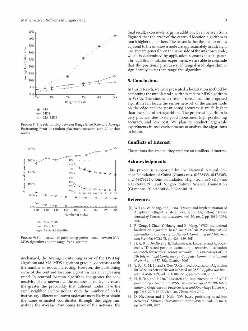

Hindawiwwwhindawicom Volume 2018
MathematicsJournal of
Hindawiwwwhindawicom Volume 2018
Mathematical Problems in Engineering
Applied MathematicsJournal of
Hindawiwwwhindawicom Volume 2018
Probability and StatisticsHindawiwwwhindawicom Volume 2018
Journal of
Hindawiwwwhindawicom Volume 2018
Mathematical PhysicsAdvances in
Complex AnalysisJournal of
Hindawiwwwhindawicom Volume 2018
OptimizationJournal of
Hindawiwwwhindawicom Volume 2018
Hindawiwwwhindawicom Volume 2018
Engineering Mathematics
International Journal of
Hindawiwwwhindawicom Volume 2018
Operations ResearchAdvances in
Journal of
Hindawiwwwhindawicom Volume 2018
Function SpacesAbstract and Applied AnalysisHindawiwwwhindawicom Volume 2018
International Journal of Mathematics and Mathematical Sciences
Hindawiwwwhindawicom Volume 2018
Hindawi Publishing Corporation httpwwwhindawicom Volume 2013Hindawiwwwhindawicom
The Scientific World Journal
Volume 2018
Hindawiwwwhindawicom Volume 2018Volume 2018
Numerical AnalysisNumerical AnalysisNumerical AnalysisNumerical AnalysisNumerical AnalysisNumerical AnalysisNumerical AnalysisNumerical AnalysisNumerical AnalysisNumerical AnalysisNumerical AnalysisNumerical AnalysisAdvances inAdvances in Discrete Dynamics in
Nature and SocietyHindawiwwwhindawicom Volume 2018
Hindawiwwwhindawicom
Dierential EquationsInternational Journal of
Volume 2018
Hindawiwwwhindawicom Volume 2018
Decision SciencesAdvances in
Hindawiwwwhindawicom Volume 2018
AnalysisInternational Journal of
Hindawiwwwhindawicom Volume 2018
Stochastic AnalysisInternational Journal of
Submit your manuscripts atwwwhindawicom