Embed Size (px)
Citation preview

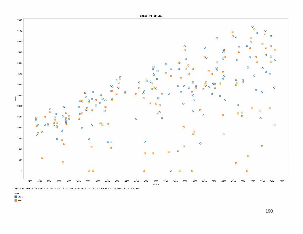
A Common-Value Auction with Liquidity NeedsA Common Value Auction with Liquidity Needs
Lawrence M. AusubelPeter Cramton
Emel Filiz-OzbayNathaniel HigginsNathaniel Higgins
Erkut OzbayAndrew Stocking
University of Maryland1 November 2008
T ti thTesting the Auction Designg
Contents
• Training seminar for experiment 1g p
• Training seminar for experiment 2
• Figures from experiment 2Figures from experiment 2
• Figures from experiment 1
4

A Common Value Auction with Liquidity NeedsBidder Instructions for Experiment 1
Lawrence M. AusubelPeter Cramton
Emel Filiz-OzbayNathaniel HigginsNathaniel Higgins
Erkut OzbayAndrew Stocking
University of Maryland11 October 2008
Two formats
• Simultaneous uniform-price sealed bidp
• Simultaneous descending clock
6
Each session
• 4-bidder sealed-bid
• 8-bidder sealed-bid
• 4-bidder clock4 bidder clock
• 8-bidder clock
7
4-bidder auction
• Treasury demand is 1000 shares of each security, where y y,each share corresponds to $1 million of face value
• Each bidder has holdings of 1000 shares of each security
• At least 1 winner
8
8-bidder auction
• Treasury demand is 2000 shares of each security, where y y,each share corresponds to $1 million of face value
• Each bidder has holdings of 500 shares of each security
• At least 4 winners
9
Uniform-price sealed-bid
10
Descending-clock auction
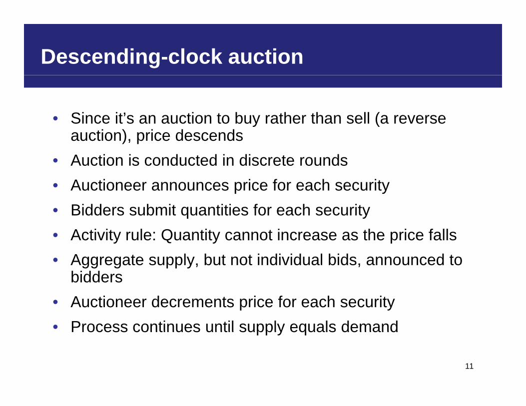
• Since it’s an auction to buy rather than sell (a reverse y (auction), price descends
• Auction is conducted in discrete rounds• Auctioneer announces price for each security• Bidders submit quantities for each security
Q f• Activity rule: Quantity cannot increase as the price falls• Aggregate supply, but not individual bids, announced to
biddersbidders• Auctioneer decrements price for each security • Process continues until supply equals demand
11
Process continues until supply equals demand

Auction mechanics
Price (cents)
R d 1
Aggregate Supply
Round 2P2
Round 1P1
Round 3P3
Round 4P4
Round 5P5
Closing Price P6Round 6
Demand Quantity (million $)
12
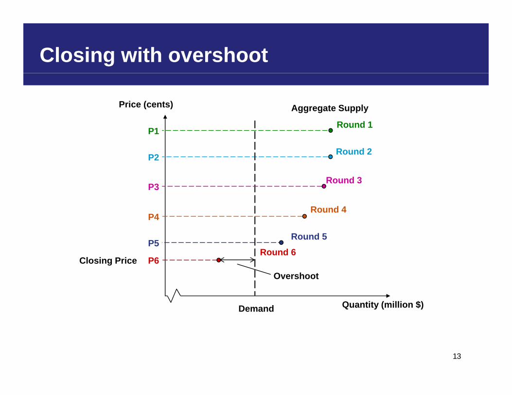
Closing with overshoot
Price (cents)
R d 1
Aggregate Supply
Round 1P1
Round 2P2
Round 3P3
Round 4P4
Closing Price P6Round 6
Round 5P5
Demand
Overshoot
Quantity (million $)
13
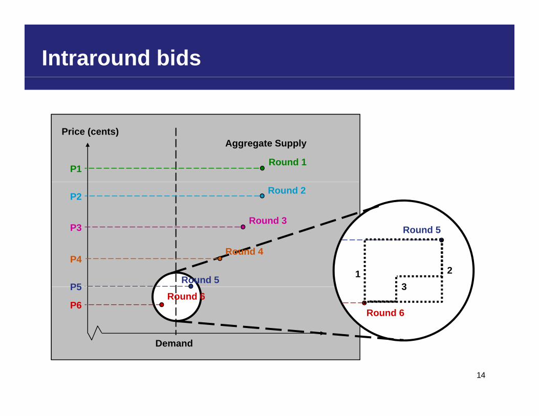
Intraround bids
P i ( t )Price (cents)
Round 1P1
Aggregate Supply
Round 5
Round 2P2
Round 3P3
Round 4P4
Round 5P5
1 23
Round 6
P5
P6Round 6
3
14
Demand
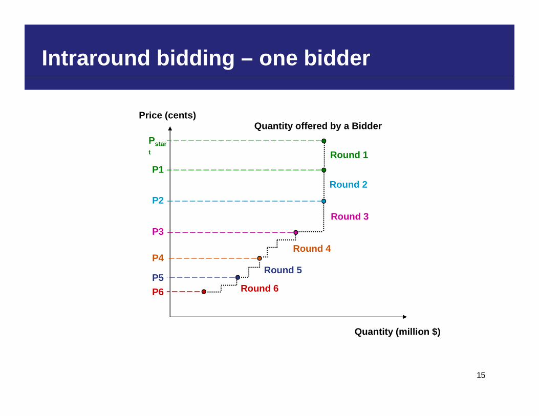
Intraround bidding – one bidder
Price (cents)Quantity offered by a Bidder
R d 2
Q y y
Round 1P1
Pstart
Round 2P2
Round 3P3
Round 4P4
P3
Round 5P5
Round 6P6 Round 6
Quantity (million $)
15
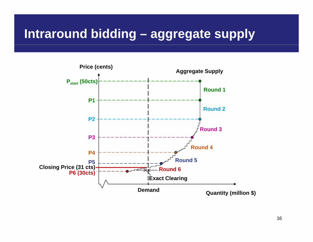
Intraround bidding – aggregate supply
Price (cents)Aggregate Supply
Round 1
P1
Pstart (50cts)
Round 2
P2
Round 3P3
Closing Price (31 cts)Round 5P5
Round 4P4
P3
Demand
Closing Price (31 cts)
Exact ClearingP6 (30cts) Round 6
Quantity (million $)
16
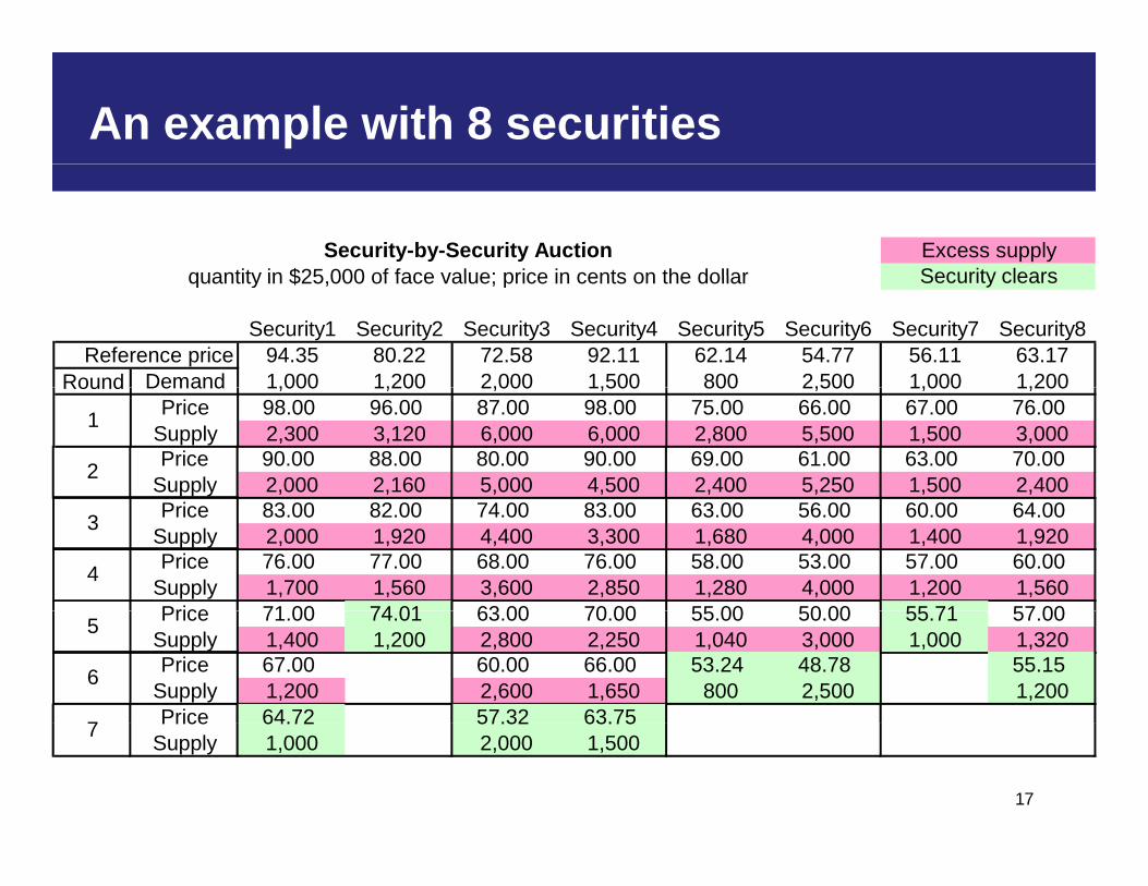
An example with 8 securities
Excess supplySecurity clears
Security-by-Security Auctionquantity in $25 000 of face value; price in cents on the dollar
Security1 Security2 Security3 Security4 Security5 Security6 Security7 Security8Reference price 94.35 80.22 72.58 92.11 62.14 54.77 56.11 63.17
Round Demand 1,000 1,200 2,000 1,500 800 2,500 1,000 1,200
Security clearsquantity in $25,000 of face value; price in cents on the dollar
Round Demand 1,000 1,200 2,000 1,500 800 2,500 1,000 1,200Price 98.00 96.00 87.00 98.00 75.00 66.00 67.00 76.00
Supply 2,300 3,120 6,000 6,000 2,800 5,500 1,500 3,0001
Price 90.00 88.00 80.00 90.00 69.00 61.00 63.00 70.00Supply 2,000 2,160 5,000 4,500 2,400 5,250 1,500 2,4002
Price 83.00 82.00 74.00 83.00 63.00 56.00 60.00 64.00Supply 2,000 1,920 4,400 3,300 1,680 4,000 1,400 1,9203
Price 76.00 77.00 68.00 76.00 58.00 53.00 57.00 60.00Supply 1,700 1,560 3,600 2,850 1,280 4,000 1,200 1,5604
Price 71 00 74 01 63 00 70 00 55 00 50 00 55 71 57 00Price 71.00 74.01 63.00 70.00 55.00 50.00 55.71 57.00Supply 1,400 1,200 2,800 2,250 1,040 3,000 1,000 1,3205
Price 67.00 60.00 66.00 53.24 48.78 55.15Supply 1,200 2,600 1,650 800 2,500 1,2006
Price 64.72 57.32 63.757
17
Price 64.72 57.32 63.75Supply 1,000 2,000 1,5007

Preferences
• Your payoff depends on your profits and how well your p y p y p yliquidity needs are met
18
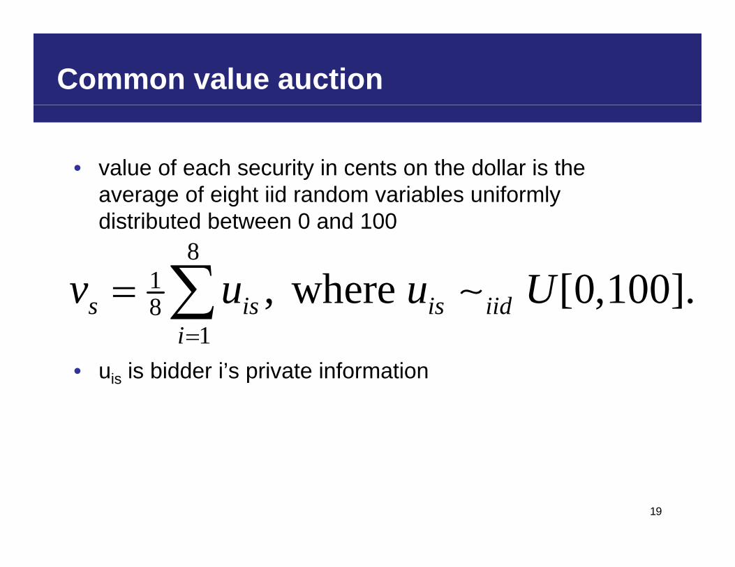
Common value auction
• value of each security in cents on the dollar is the
8
yaverage of eight iid random variables uniformly distributed between 0 and 100
818 , where [0,100].s is is iidv u u U
1i• uis is bidder i’s private information
19
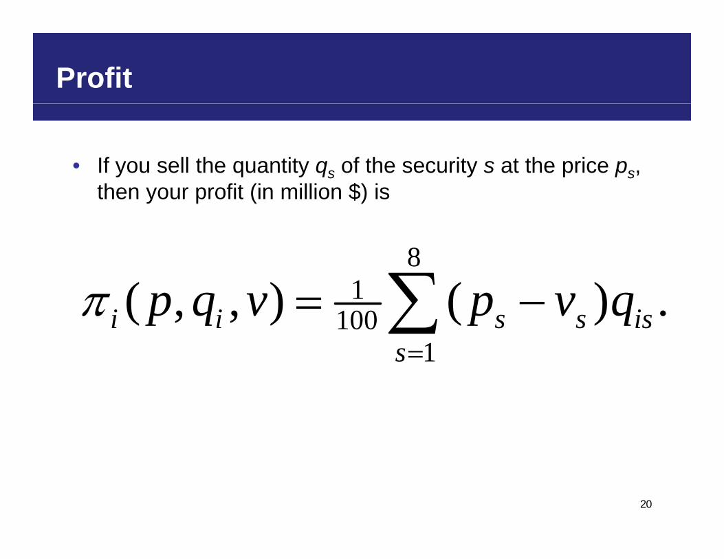
Profit
• If you sell the quantity qs of the security s at the price ps, y q y qs y p ps,then your profit (in million $) is
81
100( , , ) ( ) .i i ip q v p v q 1001
( , , ) ( ) .i i s s iss
p q v p v q
20

Liquidity need
• liquidity need, L=, which is drawn iid from the uniform q y , ,distribution on the interval [250, 750]
• You get a bonus of $1 for every dollar of sales to the Treasury up to your liquidity need of Li. You do not get any bonus for sales to the Treasury above Li. Thus, your bonus isbonus is
8 1100
1
min , .i s isL p q
21
1s

Total payoff
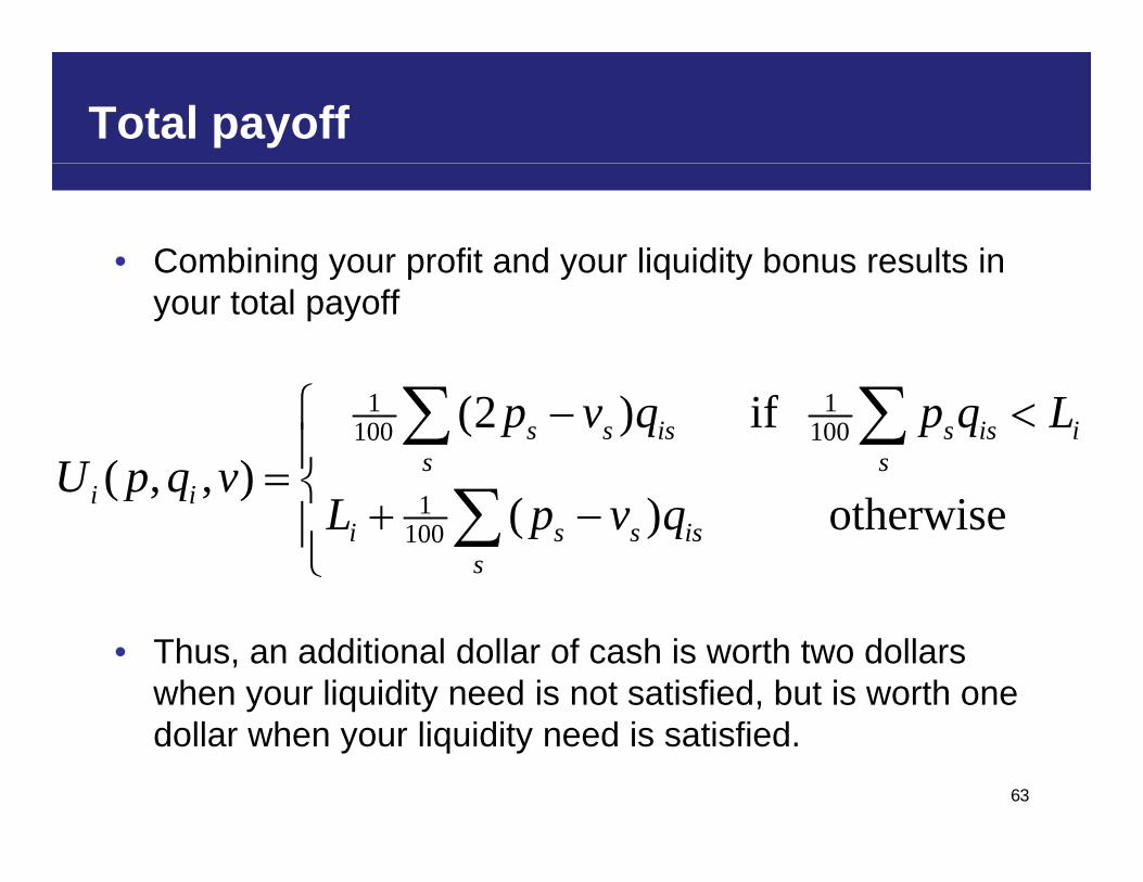
• Combining your profit and your liquidity bonus results in g y p y q yyour total payoff
8 81 1(2 ) ifp v q p q L
1 1100 100
1 18
(2 ) if ( , , )
s s is s is is s
i i
p v q p q LU p q v
1100
1( ) otherwisei s s is
sL p v q
• Thus, an additional dollar of cash is worth two dollars when your liquidity need is not satisfied, but is worth one
22
dollar when your liquidity need is satisfied.

Bidding strategy
Auction environment has three complicating features:p g
• Common value auction. You have an imperfect estimate of the good’s common value.
• Divisible good auction. Your bid is a supply curve, specifying the quantity you wish to sell at various prices.
• Liquidity need. You have a specific liquidity need that is met through selling shares from your portfolio of eight securitiessecurities.
23
Benchmark assumption
• Each bidder submits a flat supply schedule; that is, the pp y ; ,bidder offers to sell all of her holdings of a particular security at a specified price.
• Each bidder ignores her liquidity need, bidding as if Li = 0
Then we can compute an equilibrium• Then we can compute an equilibrium
• Benchmark strategy
24
Note well
• We wish to emphasize that theWe wish to emphasize that the benchmark strategy focuses on only one element of the auction Yourone element of the auction. Your challenge is to determine your own strategy to maximize your payoff thatstrategy to maximize your payoff that reflects all aspects of the auction environmentenvironment.
25

Common value distribution
81 where [0 100]v u u U 8
1, where [0,100].s is is iid
iv u u U
0.04 1
0.03
0.0350.8
0 015
0.02
0.025
PD
F
0.4
0.6
CD
F
0.005
0.01
0.015
0.2
0.4
260 50 100
0
0.005
Common Value0 50 100
0
Common Value
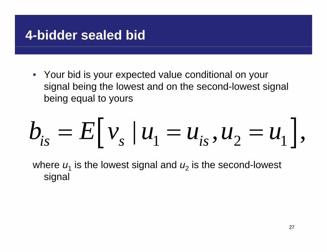
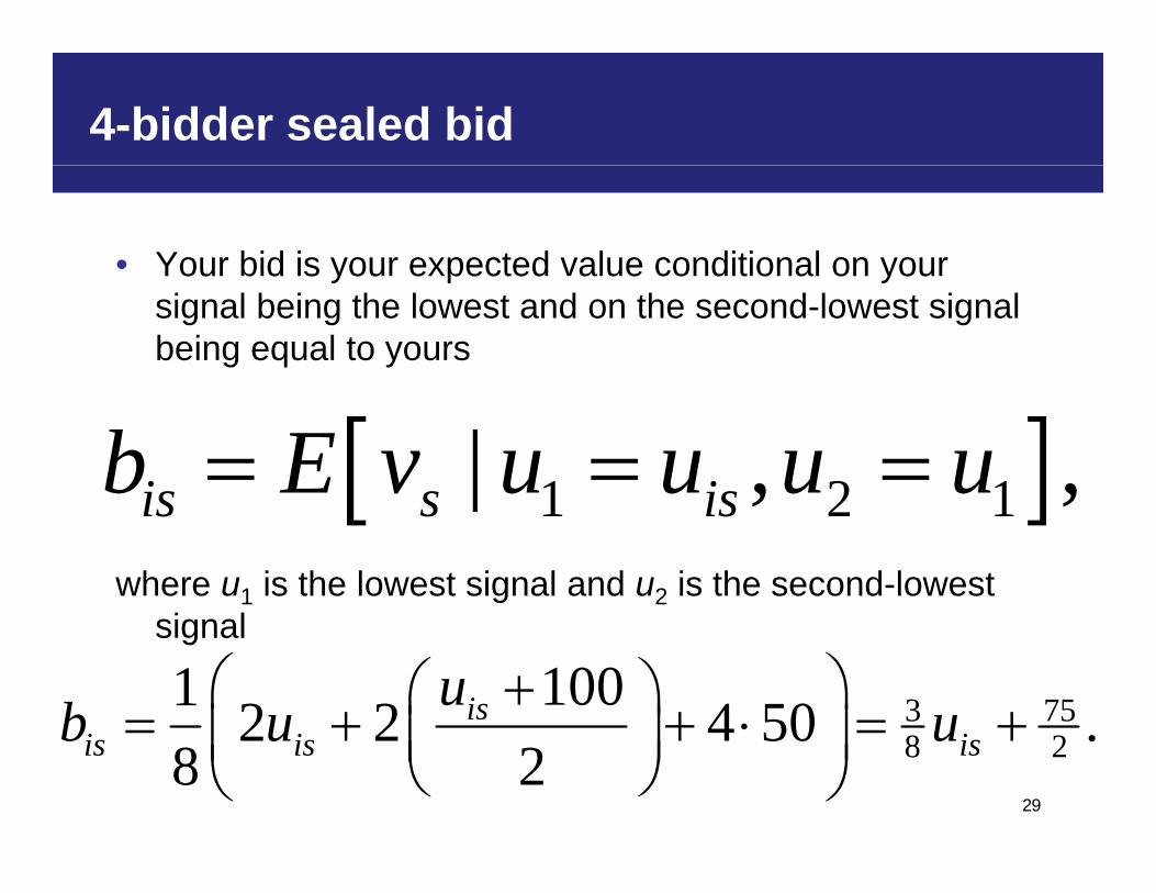
4-bidder sealed bid
• Your bid is your expected value conditional on your y p ysignal being the lowest and on the second-lowest signal being equal to yours
1 2 1| , ,is s isb E v u u u u where u1 is the lowest signal and u2 is the second-lowest
i l
1 2 1| , ,is s is
signal
27
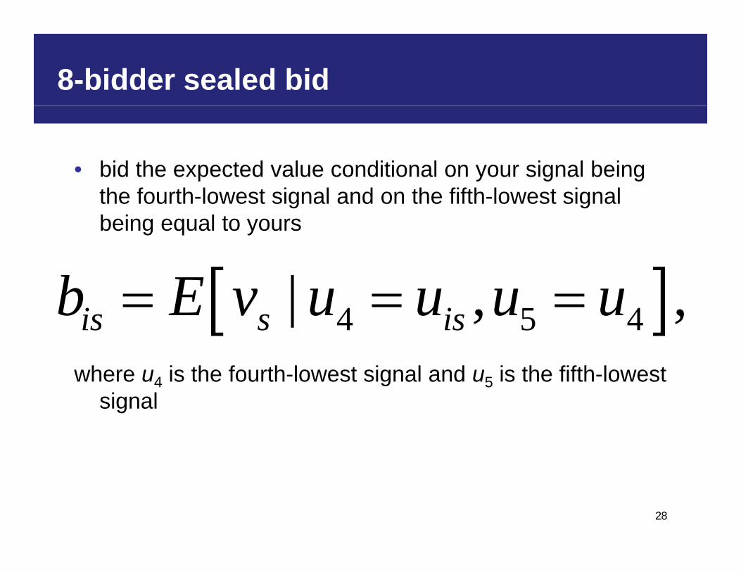
8-bidder sealed bid
• bid the expected value conditional on your signal being p y g gthe fourth-lowest signal and on the fifth-lowest signal being equal to yours
4 5 4| , ,is s isb E v u u u u where u4 is the fourth-lowest signal and u5 is the fifth-lowest
i l
4 5 4| , ,is s is
signal
28
4-bidder sealed bid
• Your bid is your expected value conditional on your y p ysignal being the lowest and on the second-lowest signal being equal to yours
1 2 1| , ,is s isb E v u u u u where u1 is the lowest signal and u2 is the second-lowest
i l
1 2 1| , ,is s is
signal
3 751001 2 2 4 50isub u u 29
8 22 2 4 50 .8 2is is isb u u
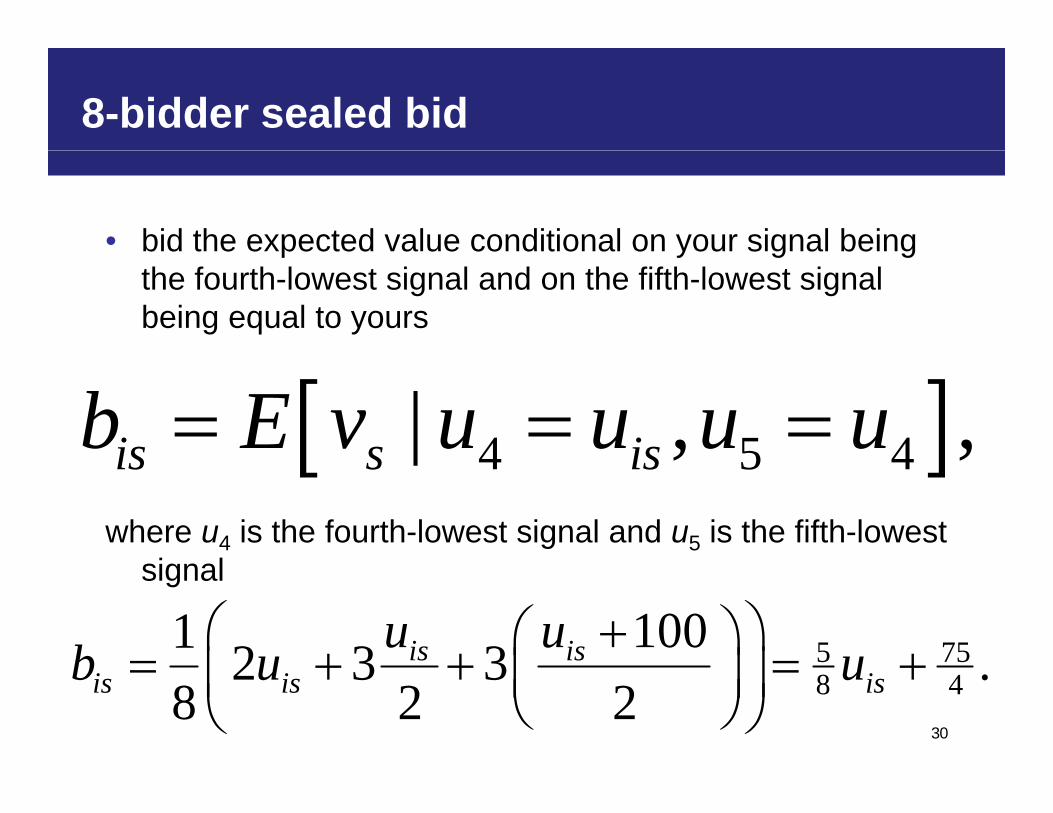
8-bidder sealed bid
• bid the expected value conditional on your signal being p y g gthe fourth-lowest signal and on the fifth-lowest signal being equal to yours
4 5 4| , ,is s isb E v u u u u where u4 is the fourth-lowest signal and u5 is the fifth-lowest
i l
4 5 4| , ,is s is
signal
5 751001 2 3 3is isu ub u u 30
8 42 3 3 .8 2 2is is isb u u
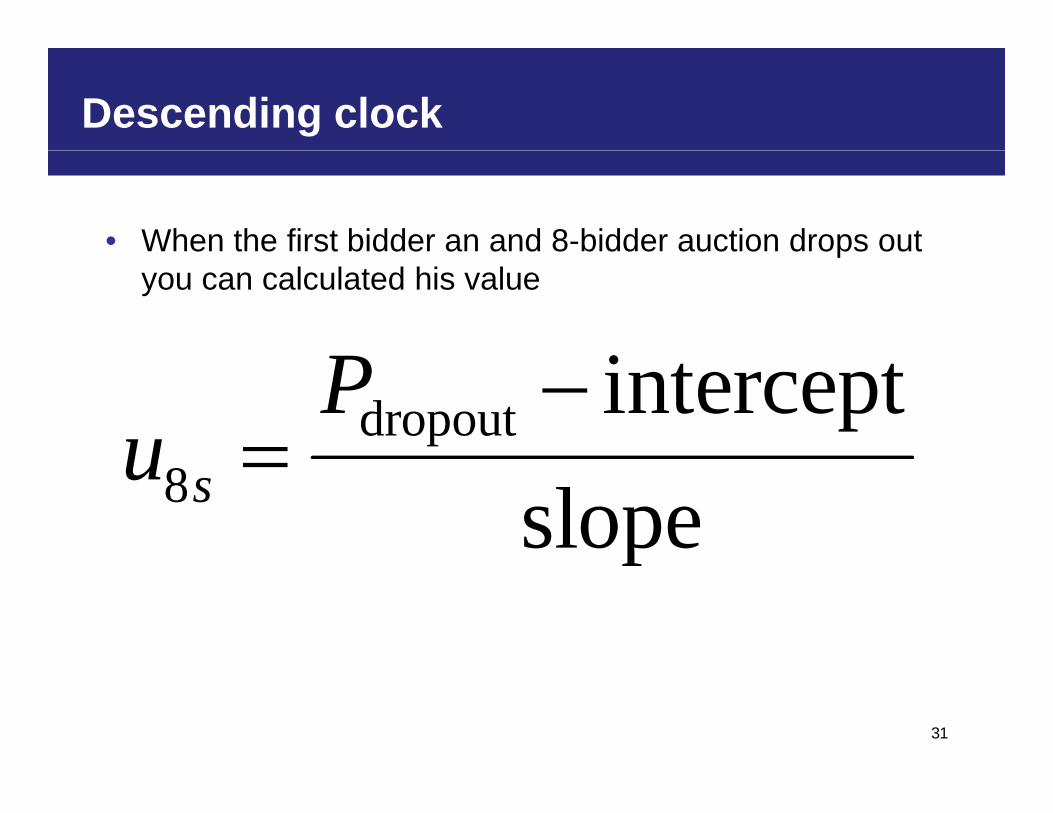
Descending clock
• When the first bidder an and 8-bidder auction drops out pyou can calculated his value
iPdropout interceptPu
8 slopesu
p
31
8-bidder clock strategy
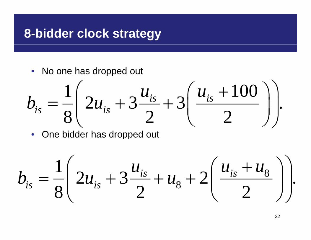
• No one has dropped outpp
1001 2 3 3is isu ub u • One bidder has dropped out
2 3 3 .8 2 2is isb u
• One bidder has dropped out
1 u u u 88
1 2 3 2 .8 2 2
is isis is
u u ub u u
32
8 2 2
8-bidder clock strategy
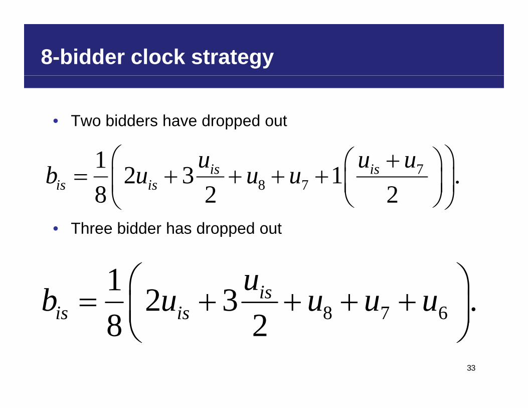
• Two bidders have dropped outpp
71 2 3 1is isu u ub u u u
• Three bidder has dropped out
8 72 3 1 .8 2 2is isb u u u
• Three bidder has dropped out
1 u 8 7 6
1 2 3 .8 2
isis is
ub u u u u
33
8 2
4-bidder clock auction
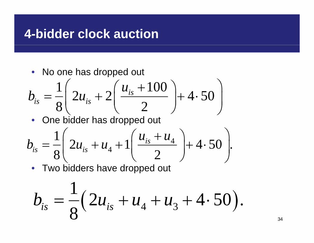
• No one has dropped outpp
1001 2 2 4 508 2
isis is
ub u
• One bidder has dropped out
1 u u
8 2
• Two bidders have dropped out
44
1 2 1 4 50 .8 2
isis is
u ub u u
• Two bidders have dropped out
1 2 4 50b u u u 34
4 32 4 50 .8is isb u u u
Moving beyond the benchmark strategy
• Bidding tool is set up to calculate the conditional g pexpected values assuming the benchmark strategy. Of course, you (and others) may well deviate from the benchmark strategy as a result of liquidity needs or otherbenchmark strategy as a result of liquidity needs or other reasons, since these other factors are ignored in the benchmark calculation
• Remember your overall goal is to maximize your experimental payoff in each auction. You should think carefully about what strategy is best apt to achieve thiscarefully about what strategy is best apt to achieve this goal.
35
Bid toolBid tool
Auction systemAuction system
A Common-Value Reference-Price Auctionwith Liquidity Needs:with Liquidity Needs:
Bidder Instructions for Experiment 2
Lawrence M. AusubelPeter Cramton
Emel Filiz-OzbayNathaniel HigginsNathaniel Higgins
Erkut OzbayAndrew Stocking
University of Maryland20 October 2008
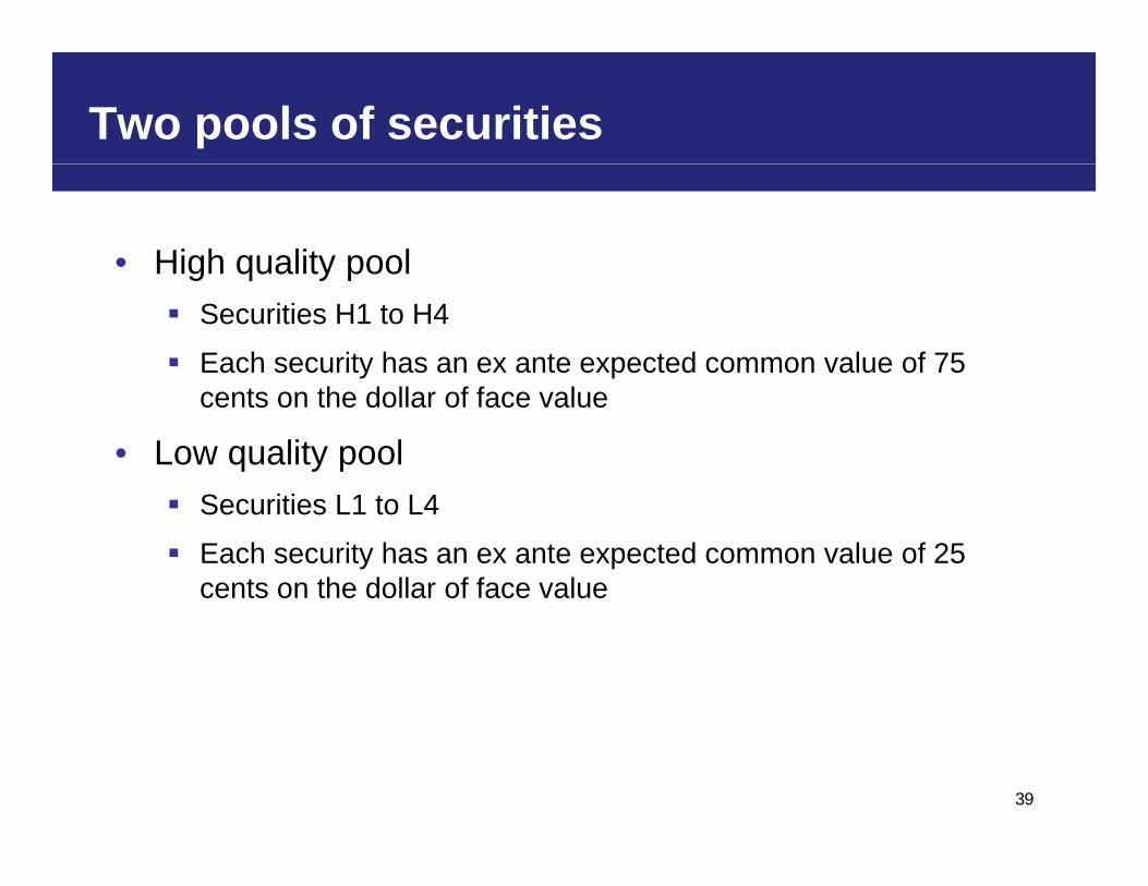
Two pools of securities
• High quality poolg q y p Securities H1 to H4
Each security has an ex ante expected common value of 75 t th d ll f f lcents on the dollar of face value
• Low quality poolSec rities L1 to L4 Securities L1 to L4
Each security has an ex ante expected common value of 25 cents on the dollar of face value
39
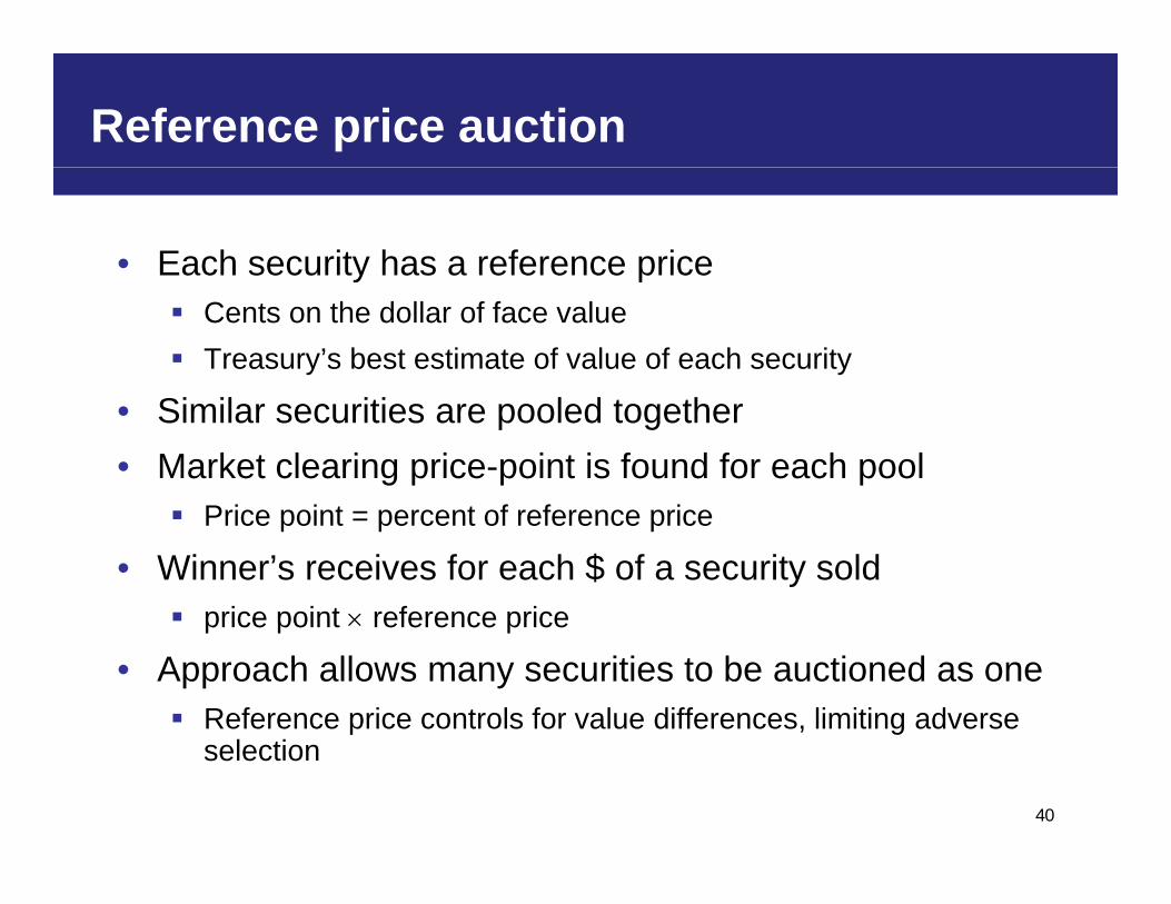
Reference price auction
• Each security has a reference pricey p Cents on the dollar of face value Treasury’s best estimate of value of each security
• Similar securities are pooled together• Market clearing price-point is found for each pool
P i i t t f f i Price point = percent of reference price
• Winner’s receives for each $ of a security sold price point reference priceprice point reference price
• Approach allows many securities to be auctioned as one Reference price controls for value differences, limiting adverse
40
selection
Two formats
• Simultaneous uniform-price sealed bidp
• Simultaneous descending clock
41
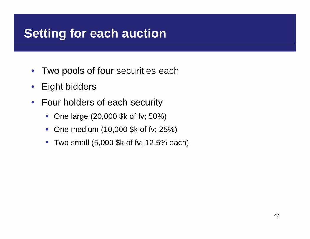
Setting for each auction
• Two pools of four securities eachp
• Eight bidders
• Four holders of each securityFour holders of each security One large (20,000 $k of fv; 50%)
One medium (10,000 $k of fv; 25%)
Two small (5,000 $k of fv; 12.5% each)
42
Each session has four auctions; Tue & Thu
1. Sealed-bid with more precise reference pricesp p
2. Clock with more precise reference prices Same signals as in prior sealed-bidg p
3. Sealed-bid less more precise reference prices
4. Clock with less precise reference pricesp p Same signals as in prior sealed-bid
43
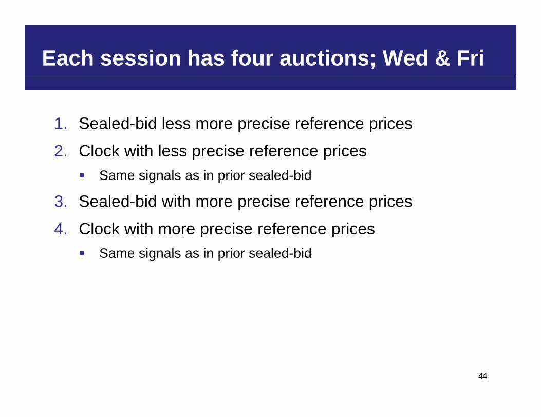
Each session has four auctions; Wed & Fri
1. Sealed-bid less more precise reference pricesp p
2. Clock with less precise reference prices Same signals as in prior sealed-bidg p
3. Sealed-bid with more precise reference prices
4. Clock with more precise reference pricesp p Same signals as in prior sealed-bid
44
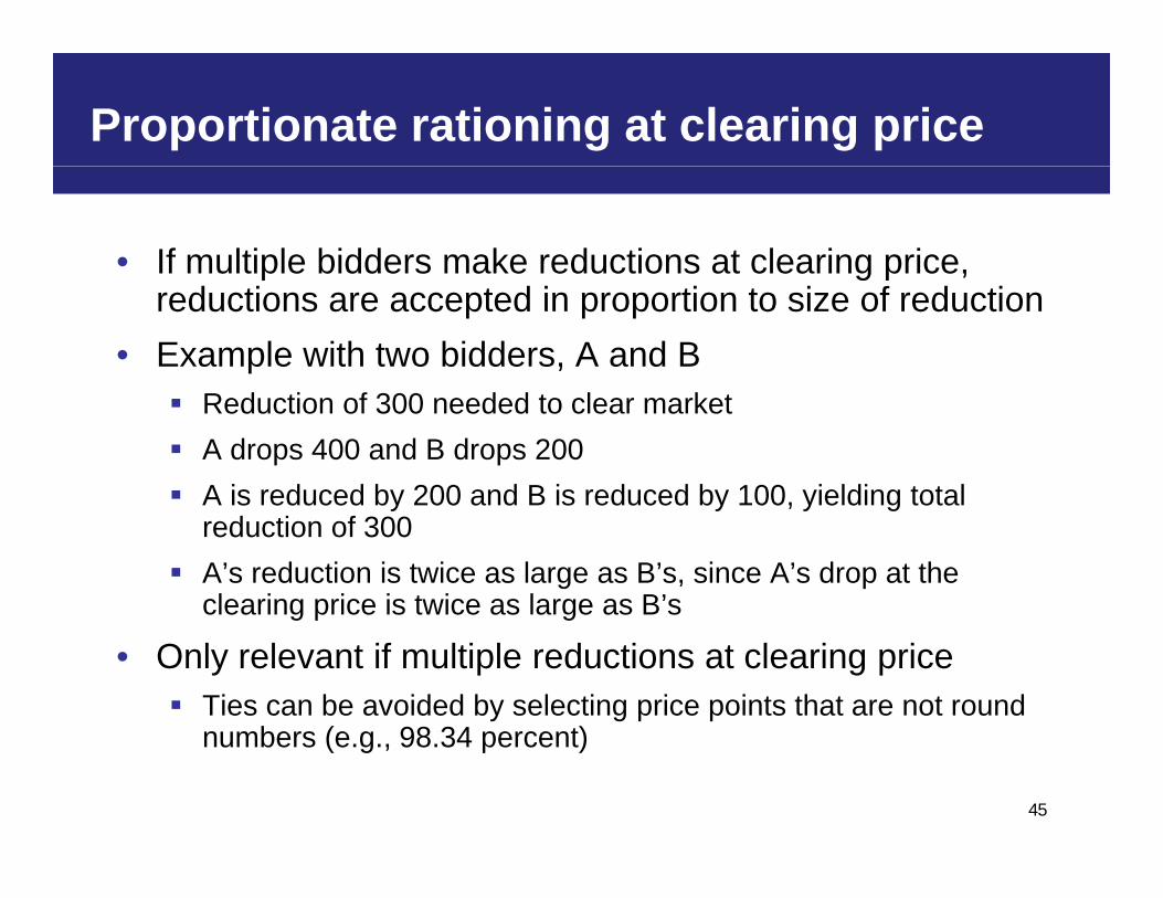
Proportionate rationing at clearing price
• If multiple bidders make reductions at clearing price, p g preductions are accepted in proportion to size of reduction
• Example with two bidders, A and BR d i f 300 d d l k Reduction of 300 needed to clear market
A drops 400 and B drops 200 A is reduced by 200 and B is reduced by 100, yielding total y y , y g
reduction of 300 A’s reduction is twice as large as B’s, since A’s drop at the
clearing price is twice as large as B’sg p g
• Only relevant if multiple reductions at clearing price Ties can be avoided by selecting price points that are not round
numbers (e g 98 34 percent)
45
numbers (e.g., 98.34 percent)
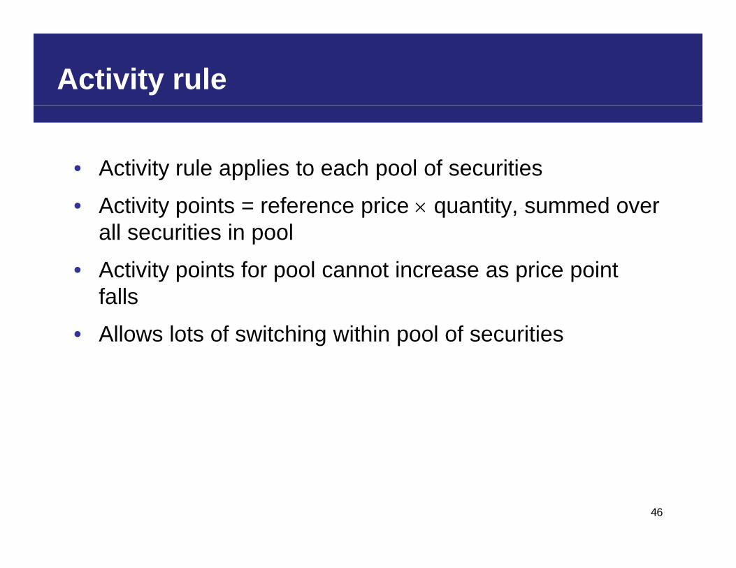
Activity rule
• Activity rule applies to each pool of securitiesy pp p
• Activity points = reference price quantity, summed over all securities in pool
• Activity points for pool cannot increase as price point falls
• Allows lots of switching within pool of securities
46
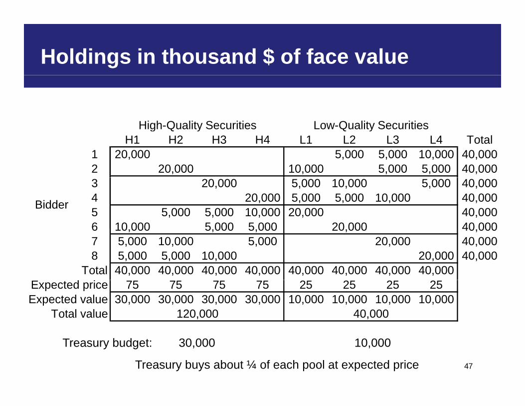
Holdings in thousand $ of face value
High-Quality Securities Low-Quality SecuritiesH1 H2 H3 H4 L1 L2 L3 L4 Total
1 20,000 5,000 5,000 10,000 40,0002 20,000 10,000 5,000 5,000 40,000
High-Quality Securities Low-Quality Securities
3 20,000 5,000 10,000 5,000 40,0004 20,000 5,000 5,000 10,000 40,0005 5,000 5,000 10,000 20,000 40,0006 10 000 5 000 5 000 20 000 40 000
Bidder
6 10,000 5,000 5,000 20,000 40,0007 5,000 10,000 5,000 20,000 40,0008 5,000 5,000 10,000 20,000 40,000
Total 40,000 40,000 40,000 40,000 40,000 40,000 40,000 40,000Expected price 75 75 75 75 25 25 25 25Expected value 30,000 30,000 30,000 30,000 10,000 10,000 10,000 10,000
Total value 120,000 40,000
47
Treasury budget: 30,000 10,000
Treasury buys about ¼ of each pool at expected price

Uniform-price sealed-bid
48
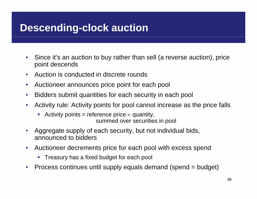
Descending-clock auction
• Since it’s an auction to buy rather than sell (a reverse auction), price i d dpoint descends
• Auction is conducted in discrete rounds• Auctioneer announces price point for each poolp p p• Bidders submit quantities for each security in each pool• Activity rule: Activity points for pool cannot increase as the price falls
Activity points = reference price quantity,summed over securities in pool
• Aggregate supply of each security, but not individual bids, announced to biddersannounced to bidders
• Auctioneer decrements price for each pool with excess spend Treasury has a fixed budget for each pool
49
• Process continues until supply equals demand (spend = budget)

Auction mechanics
Price (cents)
R d 1
Aggregate Supply
Round 2P2
Round 1P1
Round 3P3
Round 4P4
Round 5P5
Closing Price P6Round 6
Demand
Quantity ($k)
50
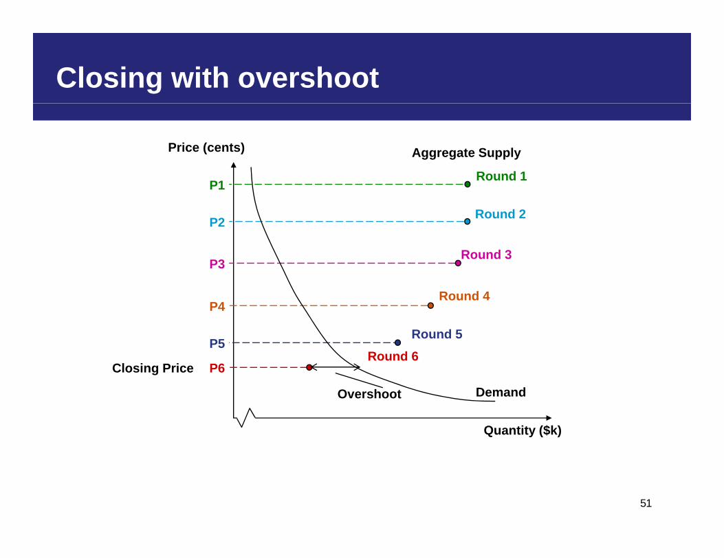
Closing with overshoot
Price (cents)
R d 1
Aggregate Supply
Round 1P1
Round 2P2
Round 3P3
Round 4P4
Closing Price P6Round 6
Round 5P5
DemandOvershoot
Quantity ($k)
51

Intraround bids
P i ( t )Price (cents)
Round 1P1
Aggregate Supply
Round 5
Round 2P2
Round 3P3
Round 4P4
Round 5P5
1 23
Round 6
P5
P6Round 6
3
Demand
52
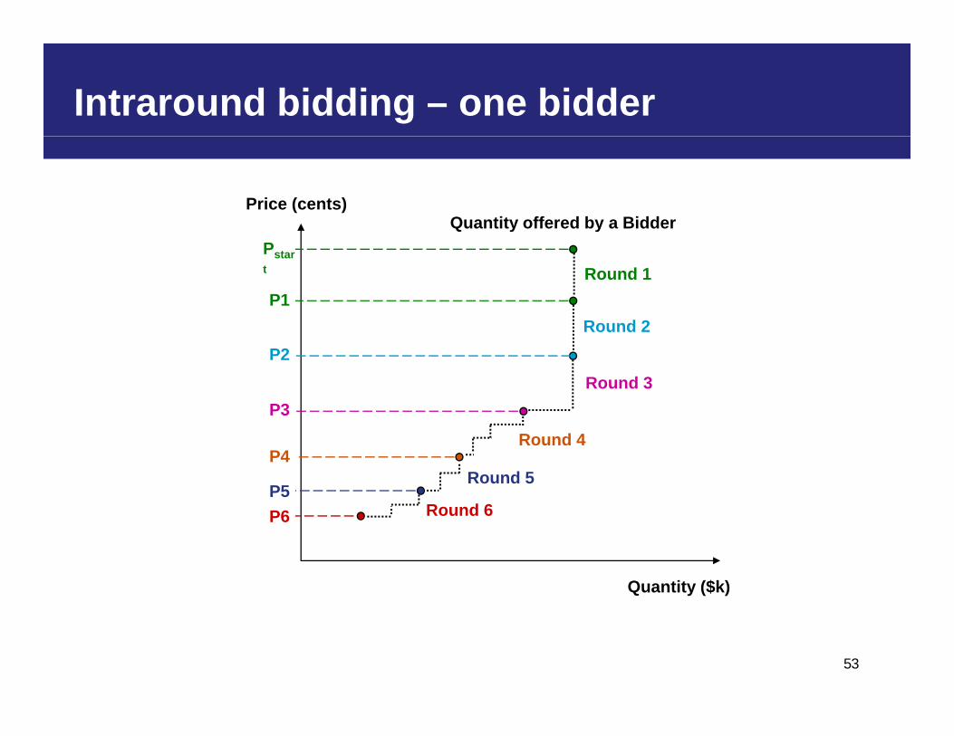
Intraround bidding – one bidder
Price (cents)Quantity offered by a Bidder
R d 2
Q y y
Round 1P1
Pstart
Round 2P2
Round 3P3
Round 4P4
P3
Round 5P5
Round 6P6 Round 6
Quantity ($k)
53
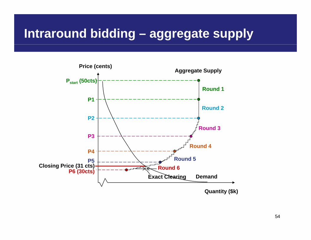
Intraround bidding – aggregate supply
Price (cents)Aggregate Supply
Round 1
P1
Pstart (50cts)
Round 2
P2
Round 3P3
Closing Price (31 cts)Round 5P5
Round 4P4
P3
Demand
Closing Price (31 cts)
Exact ClearingP6 (30cts) Round 6
Quantity ($k)
54
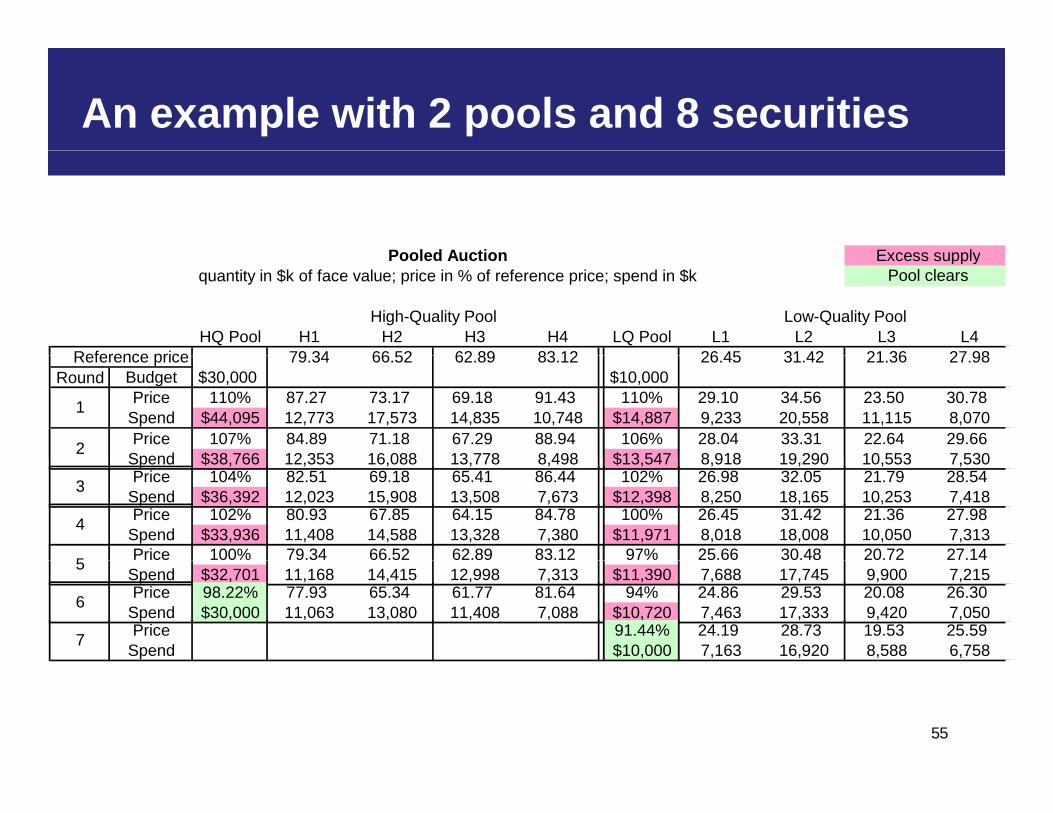
An example with 2 pools and 8 securities
Pooled Auction Excess supply
HQ Pool H1 H2 H3 H4 LQ Pool L1 L2 L3 L4Reference price 79 34 66 52 62 89 83 12 26 45 31 42 21 36 27 98
Low-Quality PoolHigh-Quality Pool
Pooled Auction Excess supplyquantity in $k of face value; price in % of reference price; spend in $k Pool clears
Reference price 79.34 66.52 62.89 83.12 26.45 31.42 21.36 27.98Round Budget $30,000 $10,000
Price 110% 87.27 73.17 69.18 91.43 110% 29.10 34.56 23.50 30.78Spend $44,095 12,773 17,573 14,835 10,748 $14,887 9,233 20,558 11,115 8,0701
Price 107% 84.89 71.18 67.29 88.94 106% 28.04 33.31 22.64 29.66Spend $38 766 12 353 16 088 13 778 8 498 $13 547 8 918 19 290 10 553 7 5302 Spend $38,766 12,353 16,088 13,778 8,498 $13,547 8,918 19,290 10,553 7,530Price 104% 82.51 69.18 65.41 86.44 102% 26.98 32.05 21.79 28.54
Spend $36,392 12,023 15,908 13,508 7,673 $12,398 8,250 18,165 10,253 7,4183
Price 102% 80.93 67.85 64.15 84.78 100% 26.45 31.42 21.36 27.98Spend $33,936 11,408 14,588 13,328 7,380 $11,971 8,018 18,008 10,050 7,3134
Price 100% 79.34 66.52 62.89 83.12 97% 25.66 30.48 20.72 27.145 Spend $32,701 11,168 14,415 12,998 7,313 $11,390 7,688 17,745 9,900 7,2155
Price 98.22% 77.93 65.34 61.77 81.64 94% 24.86 29.53 20.08 26.30Spend $30,000 11,063 13,080 11,408 7,088 $10,720 7,463 17,333 9,420 7,0506
Price 91.44% 24.19 28.73 19.53 25.59Spend $10,000 7,163 16,920 8,588 6,7587
55
Preferences
• Your payoff depends on your profits and how well your p y p y p yliquidity needs are met
56
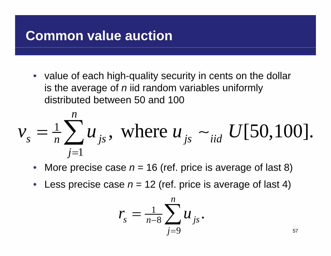
Common value auction
• value of each high-quality security in cents on the dollar g q y yis the average of n iid random variables uniformly distributed between 50 and 100
1 , where [50,100].n
s js js iidnv u u U
• More precise case n = 16 (ref. price is average of last 8)1
j jj
• Less precise case n = 12 (ref. price is average of last 4)
1n
57
18
9.s jsn
jr u
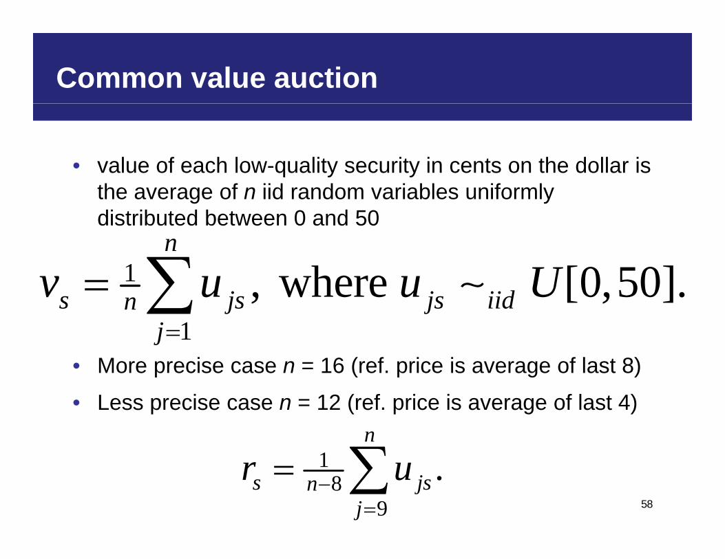
Common value auction
• value of each low-quality security in cents on the dollar is q y ythe average of n iid random variables uniformly distributed between 0 and 50
n1 , where [0,50].
n
s js js iidnv u u U
• More precise case n = 16 (ref. price is average of last 8)1j
• Less precise case n = 12 (ref. price is average of last 4)
1n
58
18
9.s jsn
jr u
Private information
• Each bidder receives 1 iid signal as private information g pfor each 5,000 of security holdings Bidder with 20,000 receives 4 private signals
Bidder with 10,000 receives 2 private signals
Bidder with 5,000 receives 1 private signal
Th th 8 i t i l i dditi t th 8• Thus, there are 8 private signals in addition to the 8 (more precise) or 4 (less precise) signals in the reference price
59
Prices
• Pool price points of pH and pL implies security prices ofp p pH pL p y p ps = pH rs for s {H1,H2,H3,H4}
ps = pL rs for s {L1,L2,L3,L4}
60
Profit
• If you sell the quantity qs of the security s at the price ps, y q y qs y p ps,then your profit (in $k) is
1( ) ( )p q v p v q 100( , , ) ( ) .i i s s iss
p q v p v q
61
Liquidity need
• liquidity need, L=, which is drawn iid from the uniform q y , ,distribution on the interval [2500, 7500]
• You get a bonus of $1 for every dollar of sales to the Treasury up to your liquidity need of Li. You do not get any bonus for sales to the Treasury above Li. Thus, your bonus isbonus is
1i L 1100min , .i s isL p q
62
s
Total payoff
• Combining your profit and your liquidity bonus results in g y p y q yyour total payoff
1 1100 100
1
(2 ) if ( , , )
s s is s is is s
i i
p v q p q LU p q v
1
100
( , , )( ) otherwisei i
i s s iss
p qL p v q
• Thus, an additional dollar of cash is worth two dollars when your liquidity need is not satisfied, but is worth one
63
dollar when your liquidity need is satisfied.

Bidding strategy
Auction environment has five complicating features:
• Common value auction. You have an imperfect estimate of the good’s common value.
• Divisible good auction Your bid is a supply curve specifying the• Divisible good auction. Your bid is a supply curve, specifying the quantity you wish to sell at various prices.
• Demand for pool of securities. Treasury does not have a demand for i di id l iti b t f l f iti (hi h d l litindividual securities, but for pools of securities (high- and low-quality pools)
• Asymmetric holdings. Bidders have different holdings of securities.
• Liquidity need. You have a specific liquidity need that is met through selling shares from your portfolio of eight securities.
64

Goal
Your challenge is to determine yourYour challenge is to determine your own strategy to maximize your payoff th t fl t ll t f th tithat reflects all aspects of the auction environment. The best response in this auction, as in any auction is a best response to what the other pbidders are actually doing.
65

Common value density: more precise case
0 2
0.25CV | 12 signals=mean
0 2
0.25CV | 10 signals=mean
0 2
0.25CV | 9 signals=mean
0.15
0.2
0.15
0.2
0.15
0.2
0.05
0.1
p
0.05
0.1
p
0.05
0.1
p
0 10 20 30 40 500
CV with 20,000 & 4 unknown signals0 10 20 30 40 50
0
CV with 10,000 & 6 unknown signals0 10 20 30 40 5
0
CV with 5,000 & 7 unknown signals
66
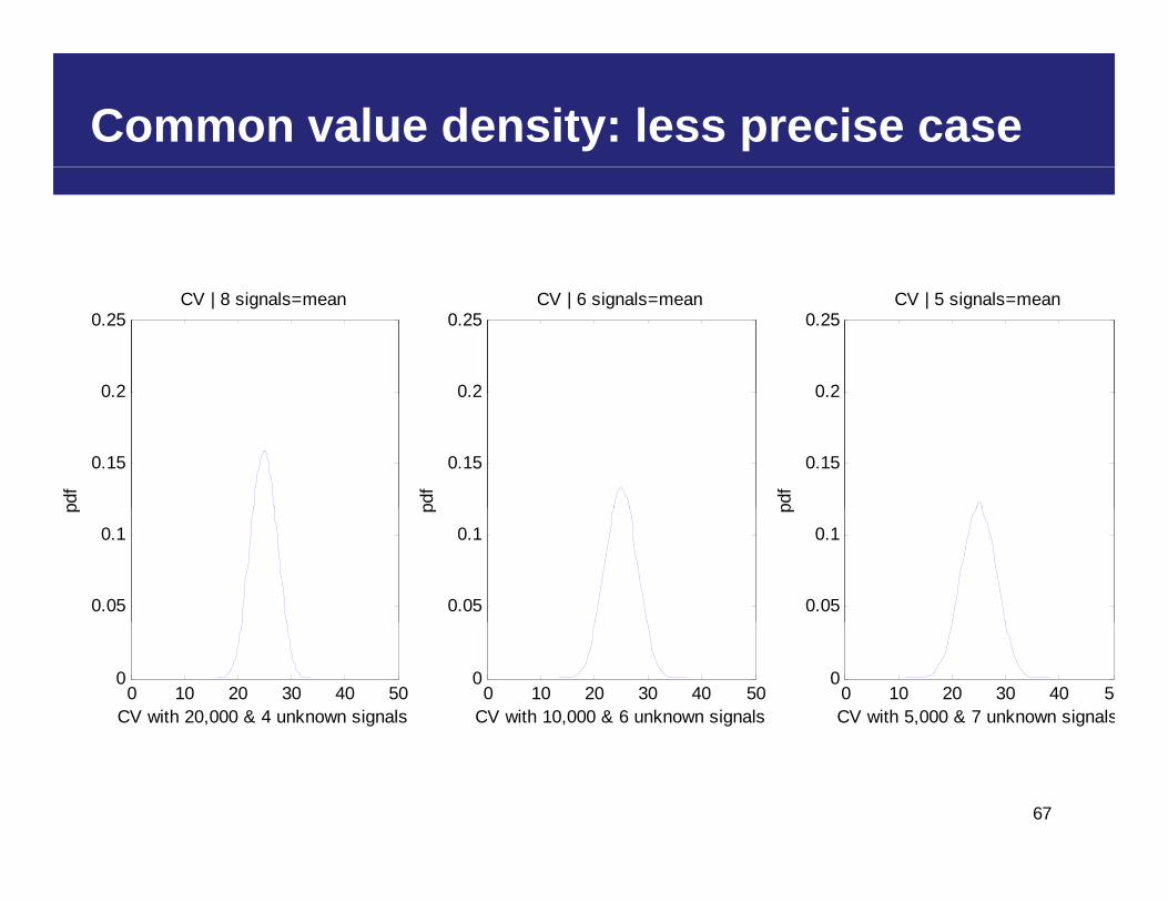
Common value density: less precise case
0 2
0.25CV | 8 signals=mean
0 2
0.25CV | 6 signals=mean
0 2
0.25CV | 5 signals=mean
0.15
0.2
0.15
0.2
0.15
0.2
0.05
0.1
p
0.05
0.1
p
0.05
0.1
p
0 10 20 30 40 500
CV with 20,000 & 4 unknown signals0 10 20 30 40 50
0
CV with 10,000 & 6 unknown signals0 10 20 30 40 50
0
CV with 5,000 & 7 unknown signals
67
Bidding tool
• Bidding tool is set up to calculate the conditional g pexpected values assuming what you know and guesses of what you don’t know
• Remember your overall goal is to maximize your experimental payoff in each auction. You should think carefully about what strategy is best apt to achieve thiscarefully about what strategy is best apt to achieve this goal.
• Take-home pay is $1 per 100 $k of experimental payoff
68
Bidding toolBidding tool

Auction systemAuction system
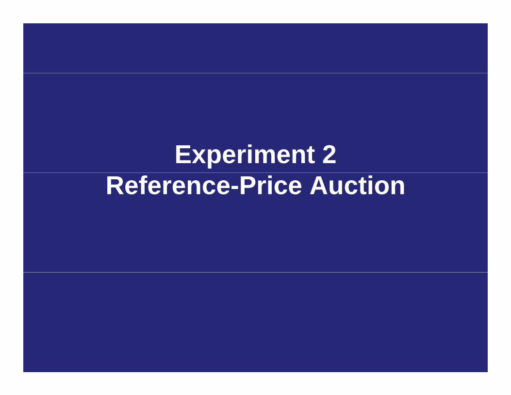
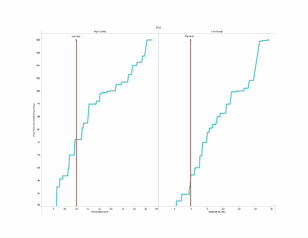
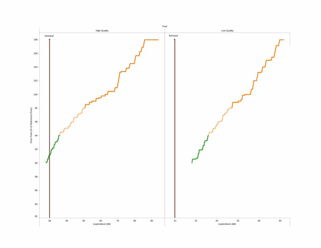
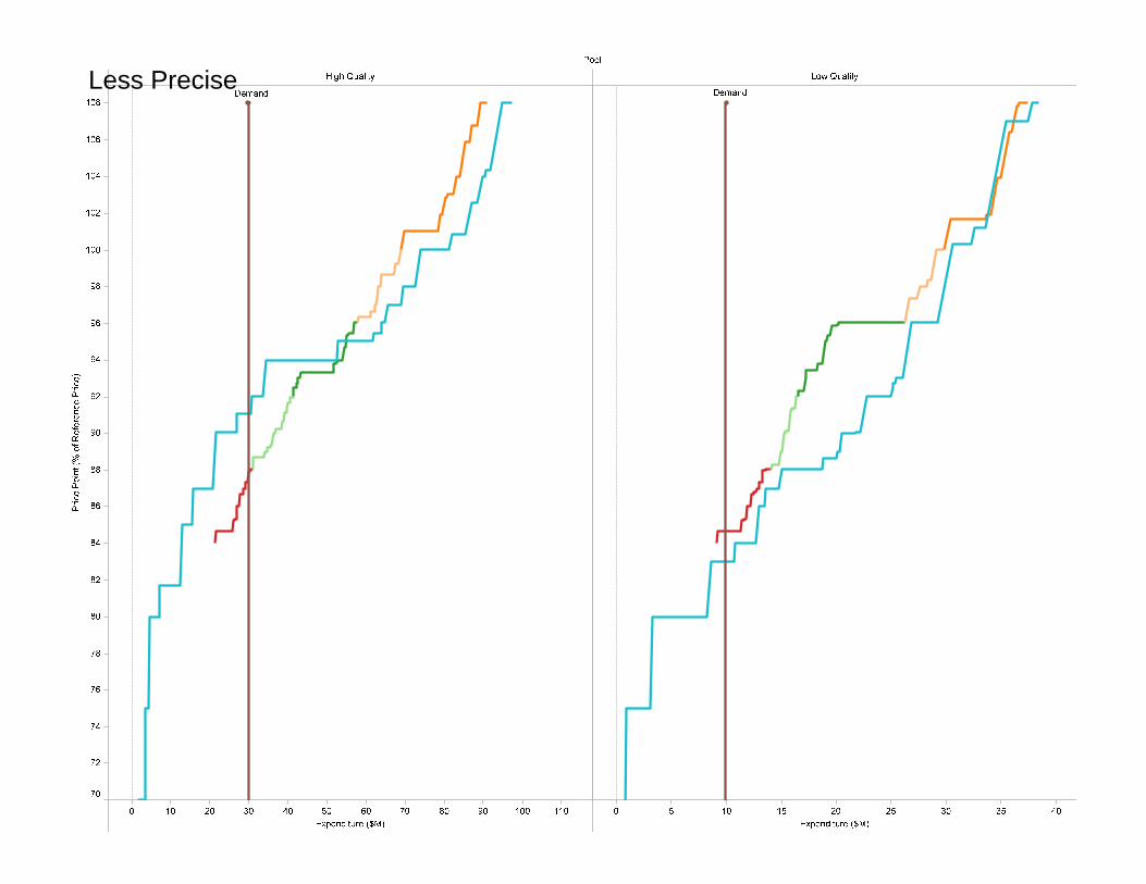
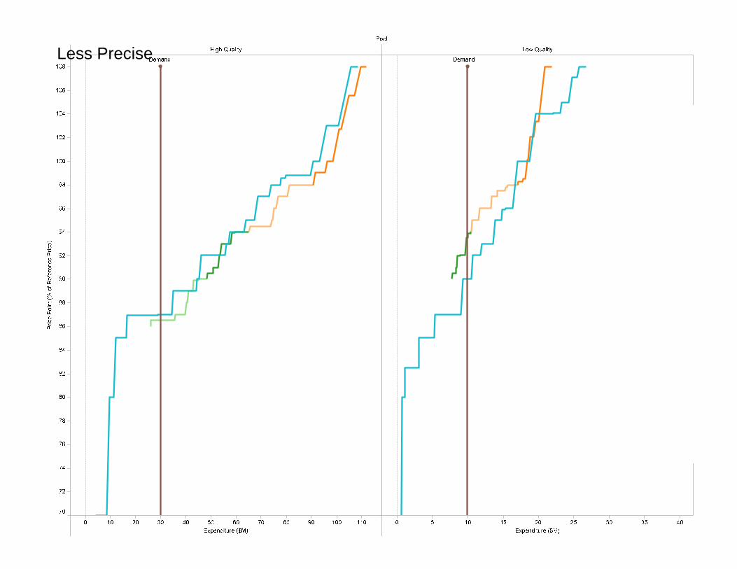
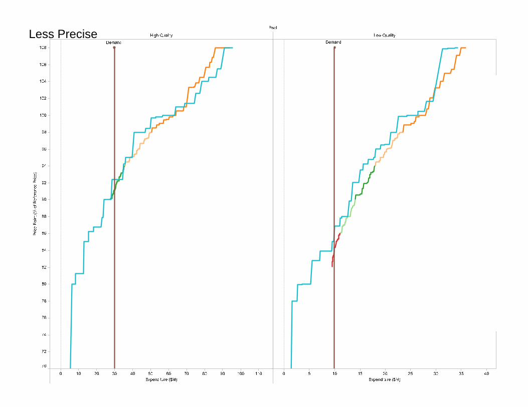
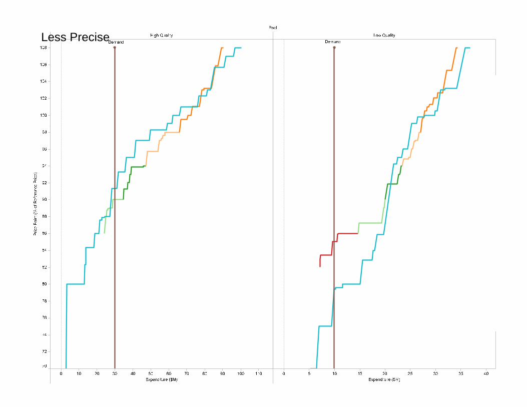
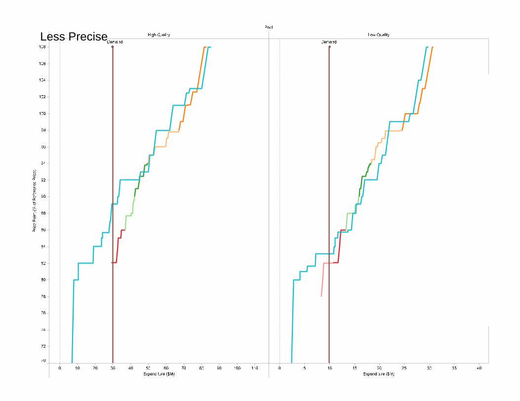
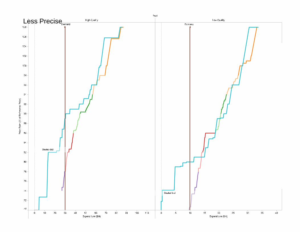
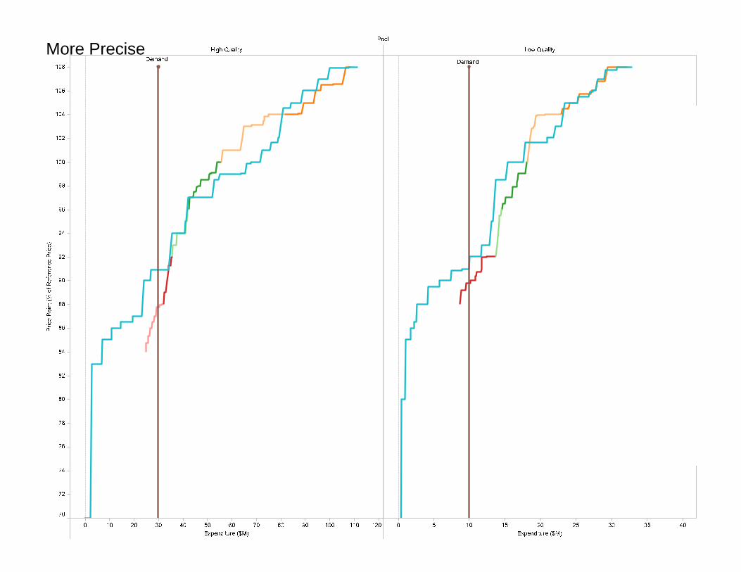
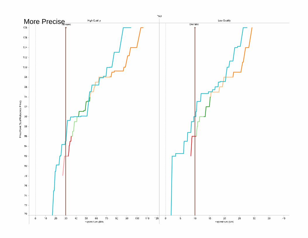
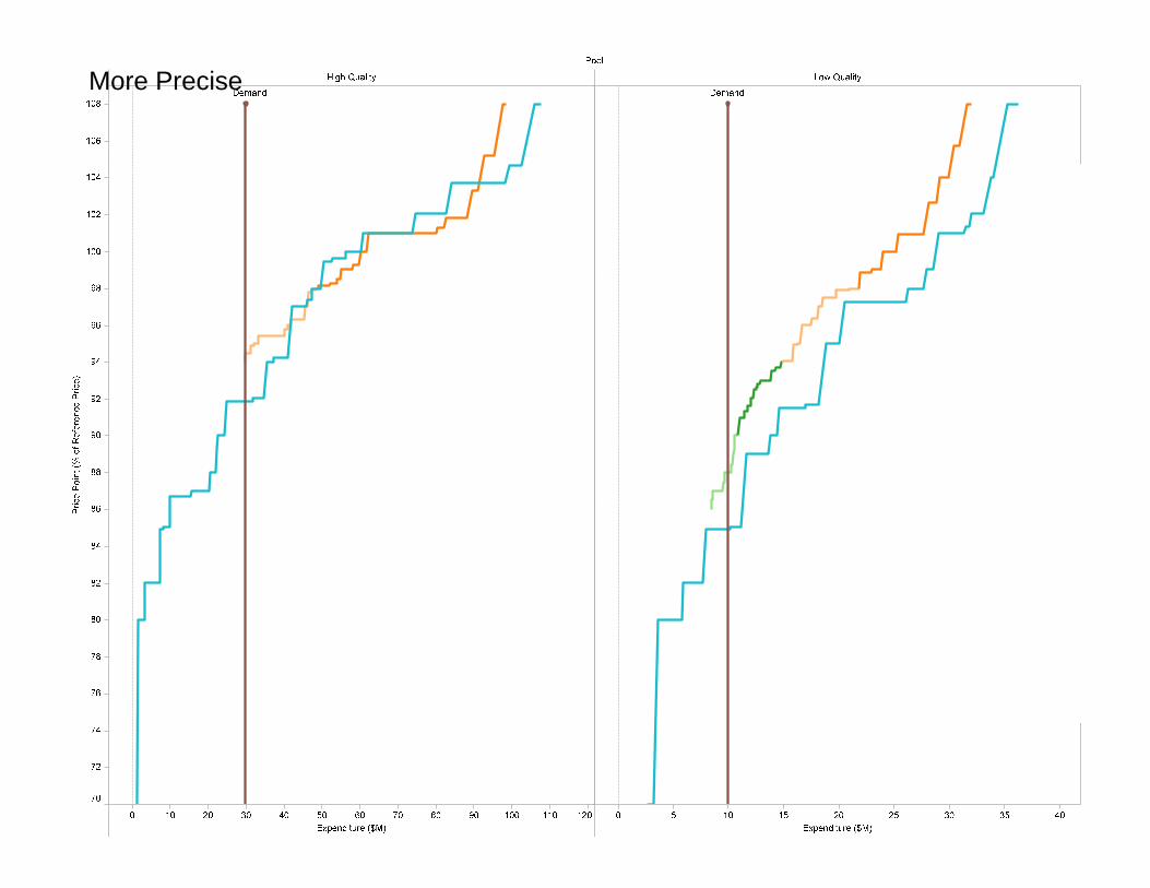
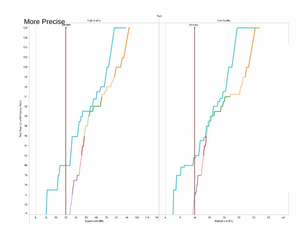
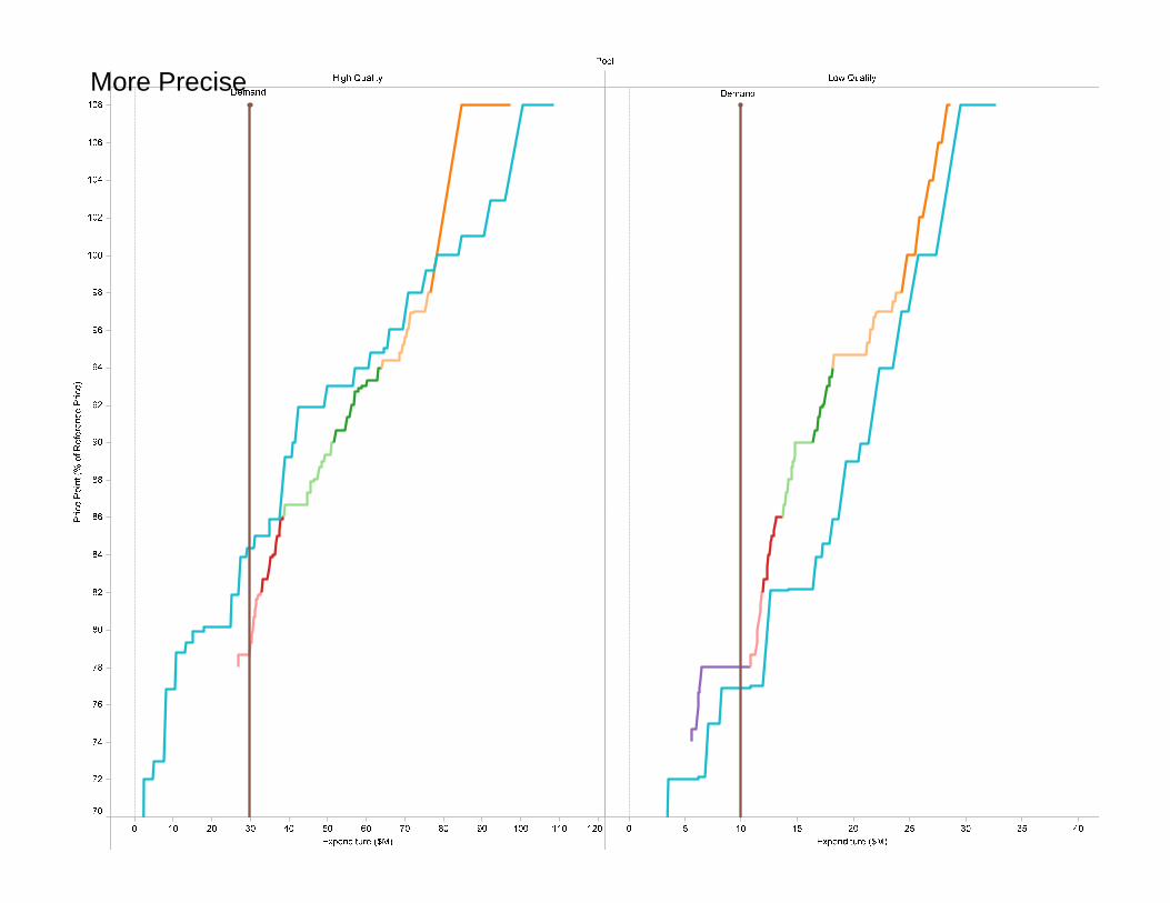
Experiment 2Reference-Price Auction
)ic
e Po
int (
% o
f Ref
eren
ce P
rice
Pri
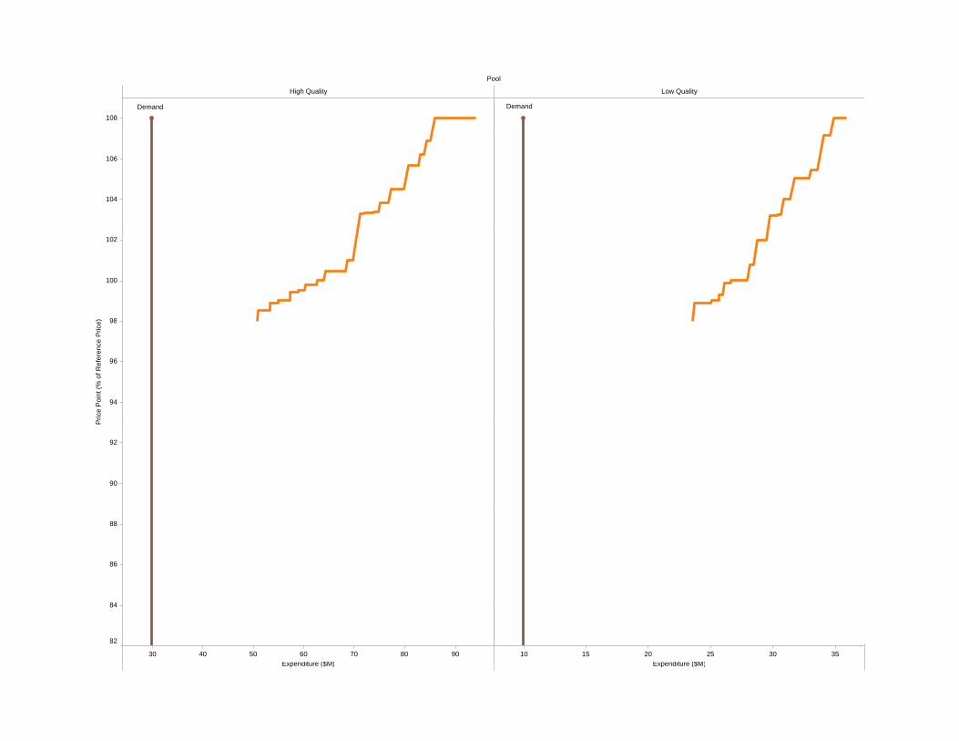
Pool
High Quality Low Quality
108Demand Demand
104
106
98
100
102
e)
94
96
ice
Poi
nt (%
of R
efer
ence
Pric
e
90
92
Pr
84
86
88
30 40 50 60 70 80 90Expenditure ($M)
10 15 20 25 30 35Expenditure ($M)
82
84
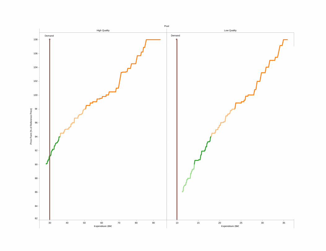
Pool
High Quality Low Quality
108Demand Demand
104
106
98
100
102
e)
94
96
ice
Poi
nt (%
of R
efer
ence
Pric
e
90
92
Pr
84
86
88
30 40 50 60 70 80 90Expenditure ($M)
10 15 20 25 30 35Expenditure ($M)
82
84
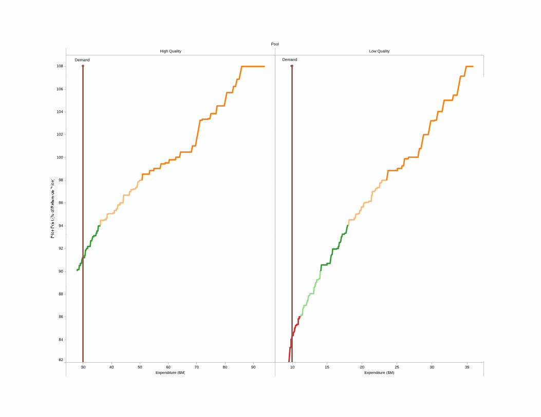
Pool
High Quality Low Quality
108Demand Demand
104
106
98
100
102
e)
94
96
98
ce P
oint
(% o
f Ref
eren
ce P
rice
90
92
Pric
86
88
30 40 50 60 70 80 90Expenditure ($M)
10 15 20 25 30 35Expenditure ($M)
82
84
Pool
High Quality Low Quality
108Demand Demand
104
106
98
100
102
e)
94
96
ce P
oint
(% o
f Ref
eren
ce P
rice
90
92
Pric
86
88
30 40 50 60 70 80 90Expenditure ($M)
10 15 20 25 30 35Expenditure ($M)
82
84
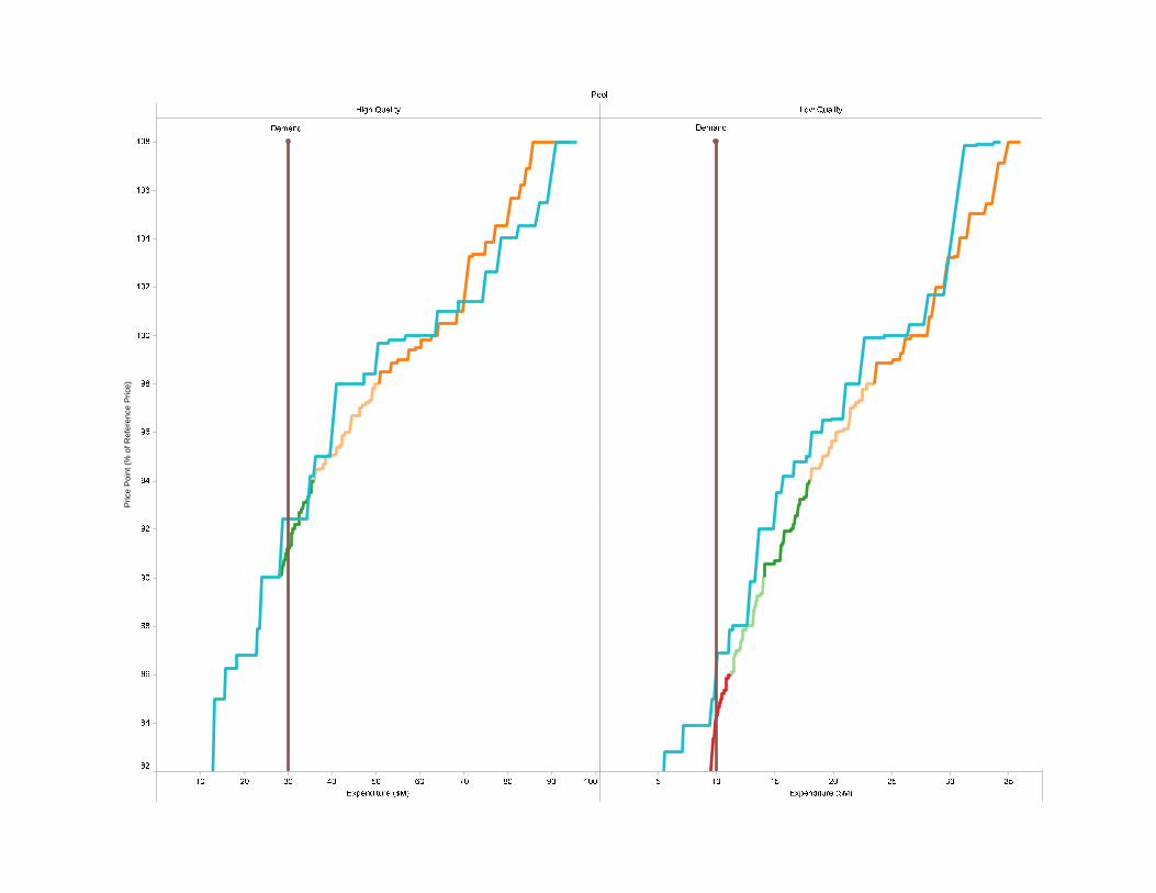
Pool
High Quality Low Quality
108Demand Demand
104
106
98
100
102
94
96
90
92
84
86
88
30 40 50 60 70 80 90Expenditure ($M)
10 15 20 25 30 35Expenditure ($M)
82
84
ce)
Pric
e P
oint
(% o
f Ref
eren
ce P
ricP

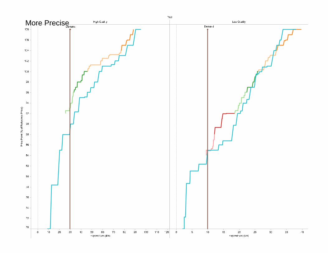
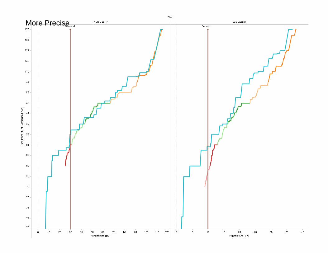
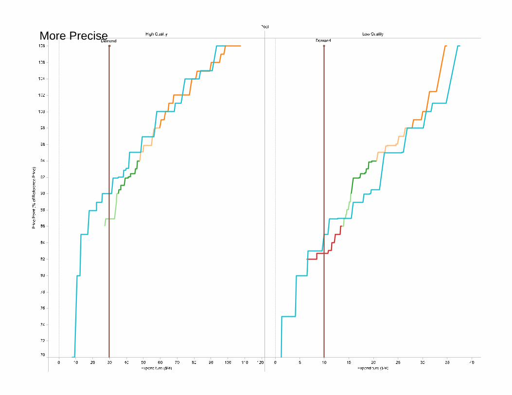
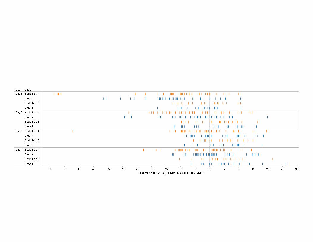
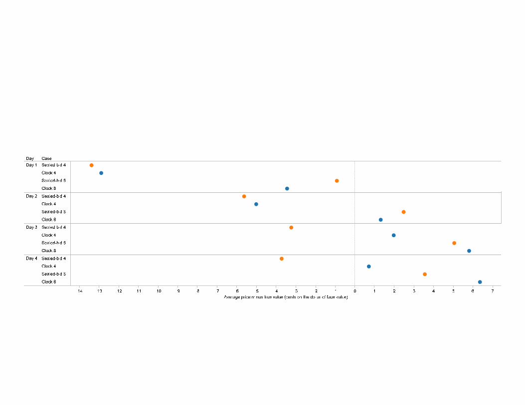
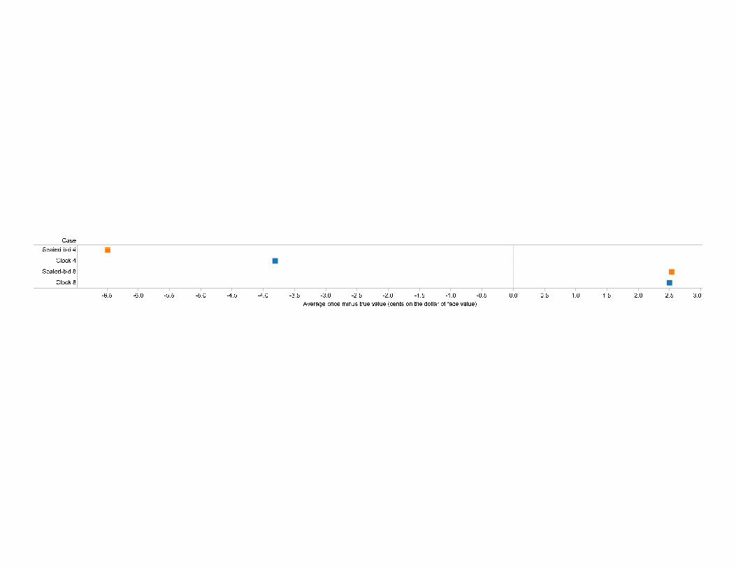
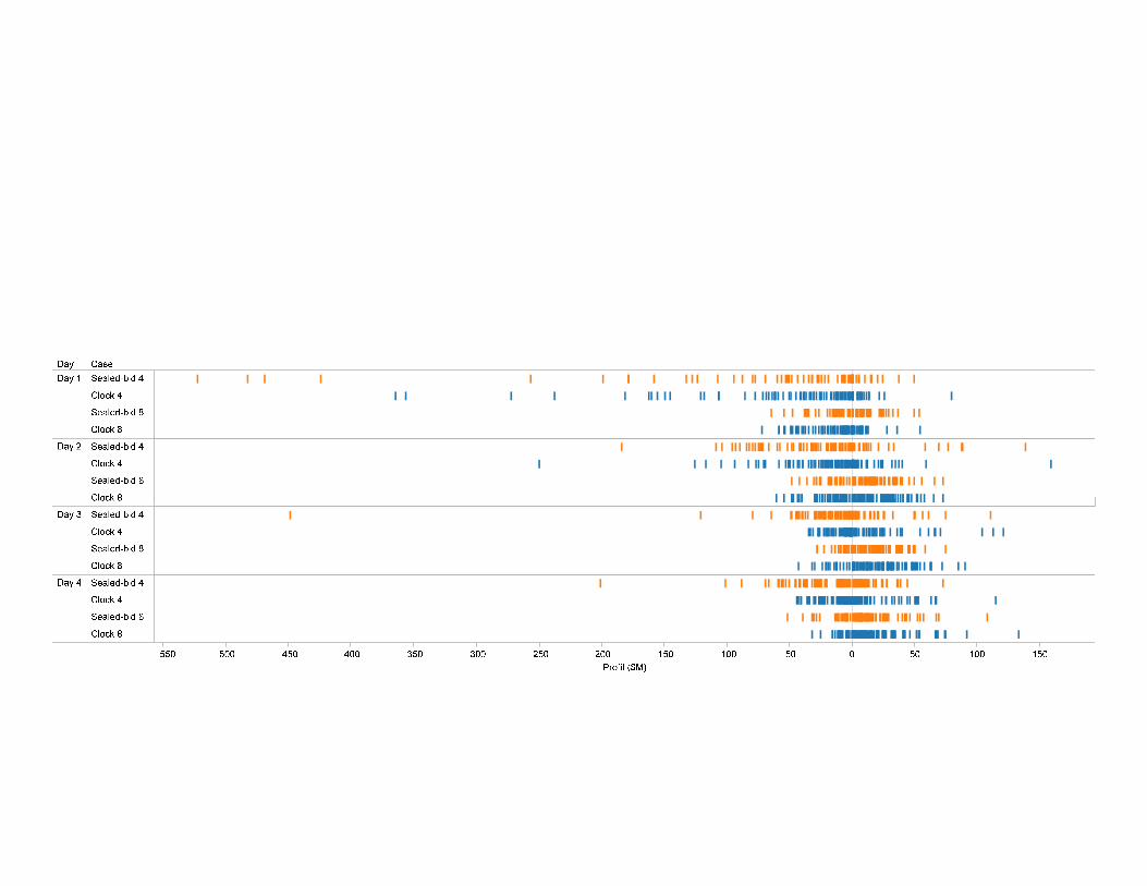
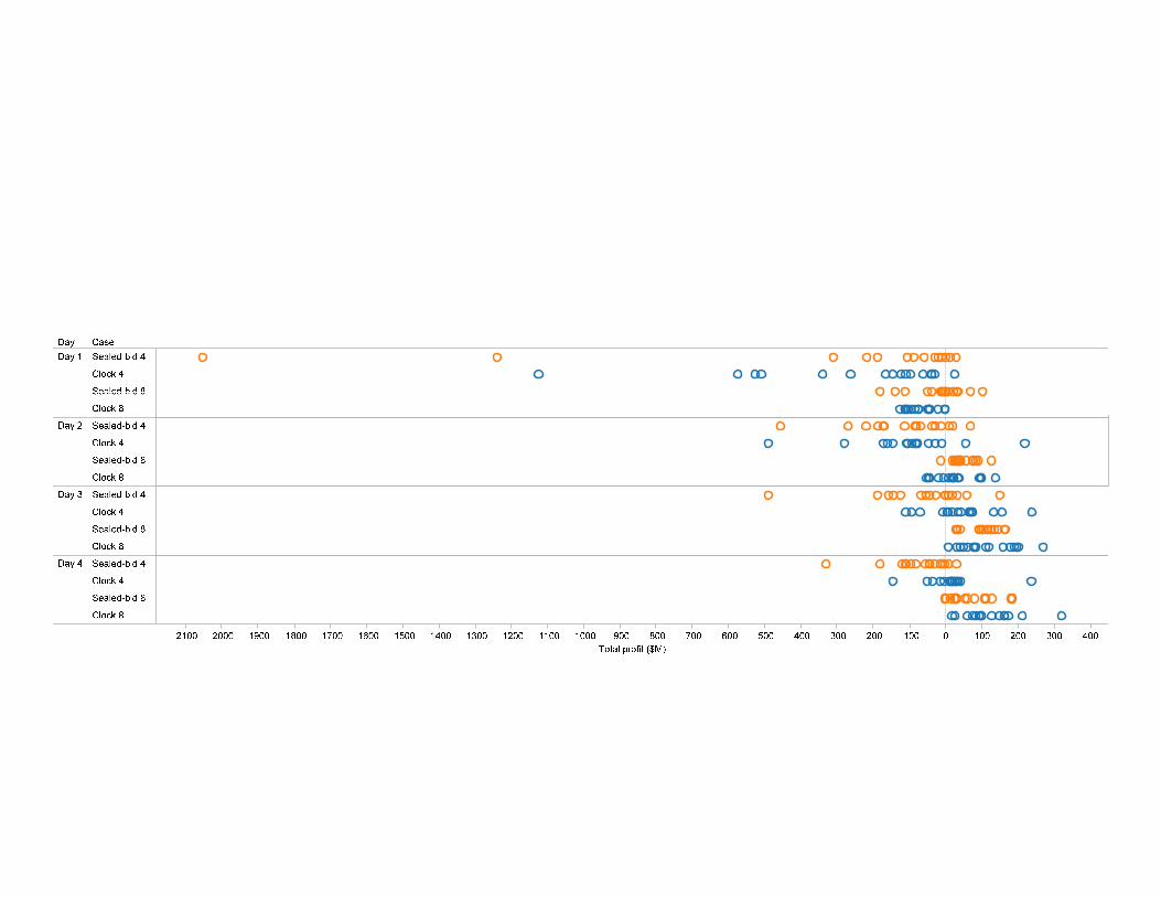
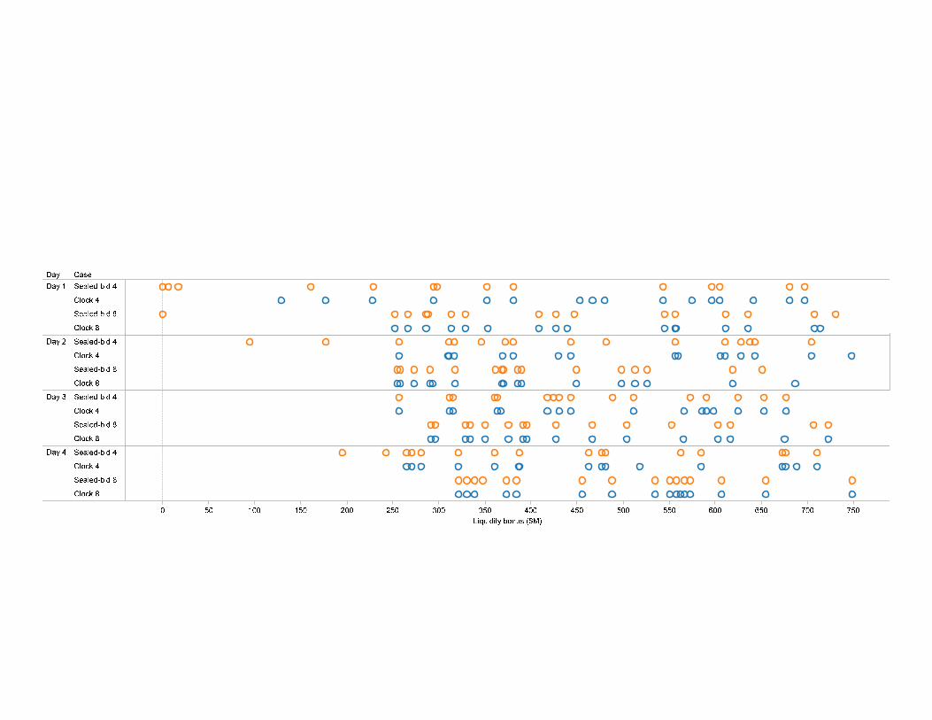
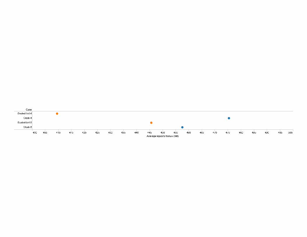
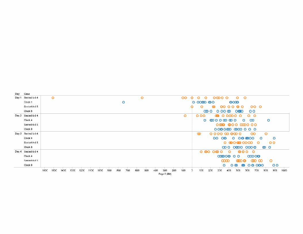
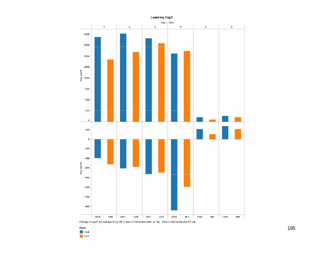
Results
• Does it work?
• Can it be implemented quickly?

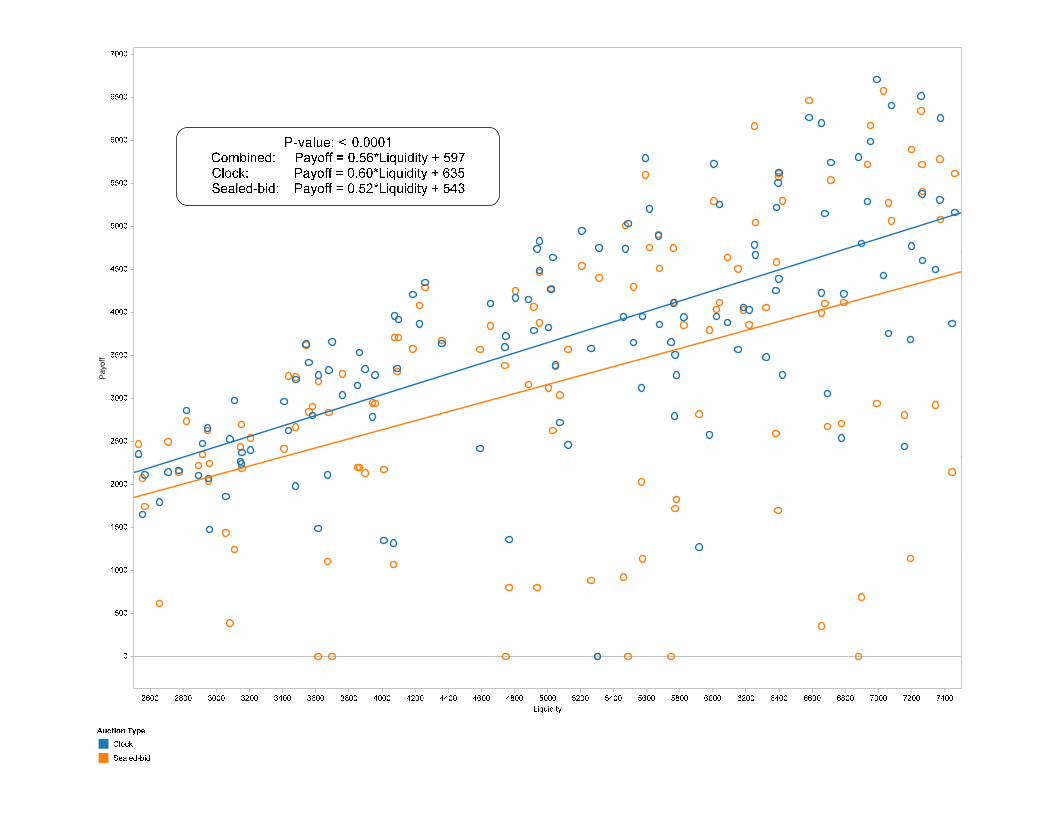
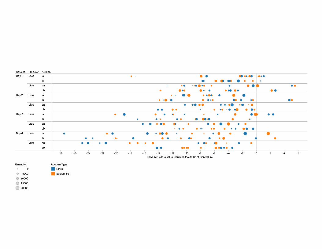
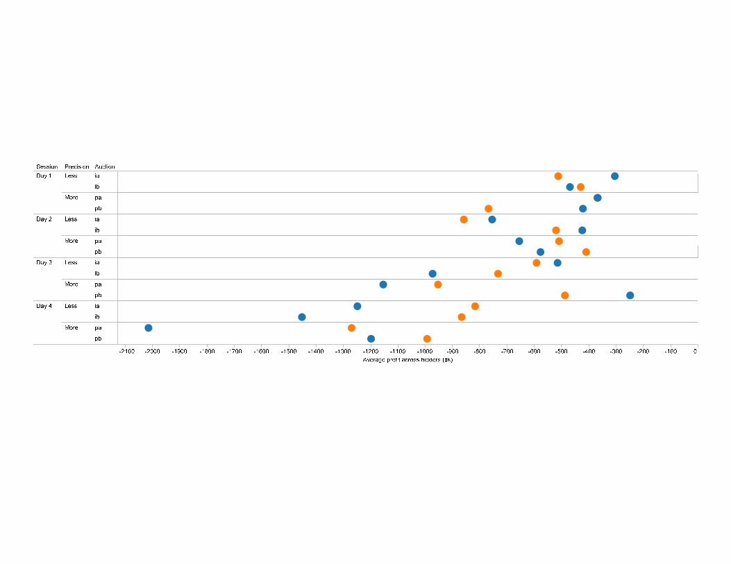
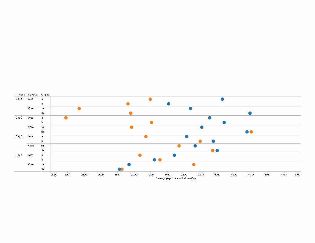
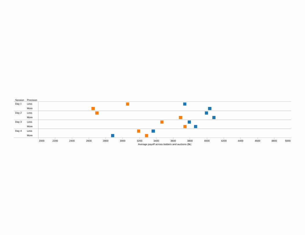
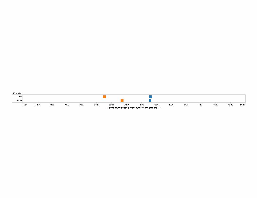
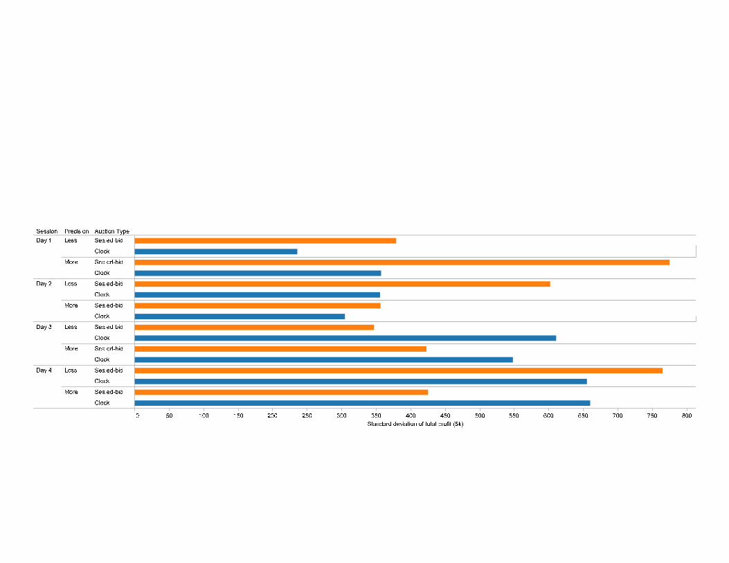
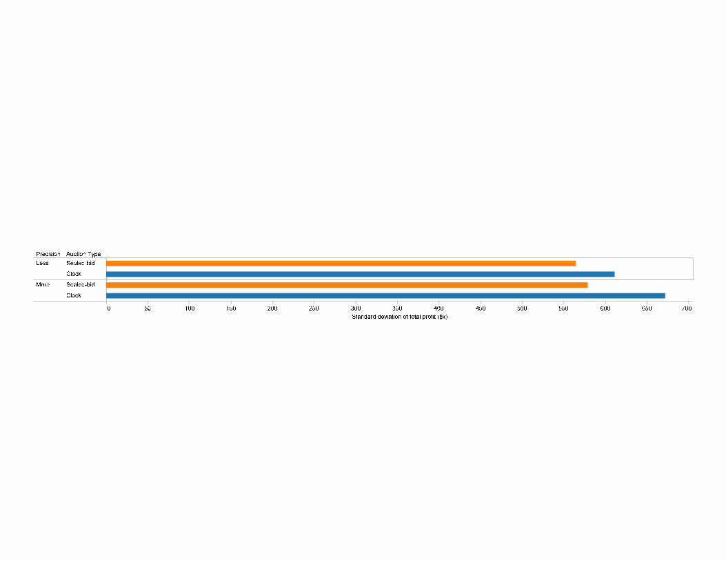
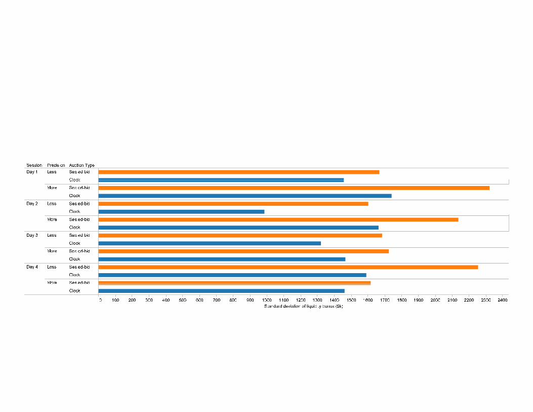
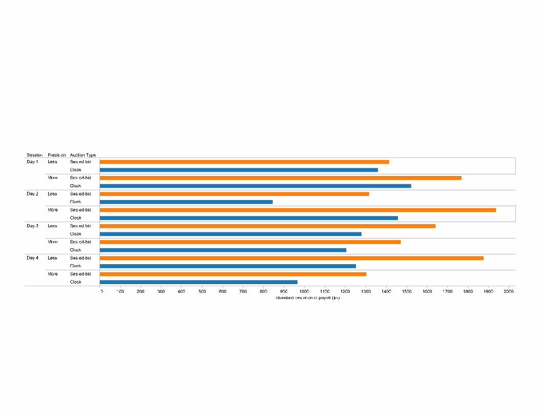
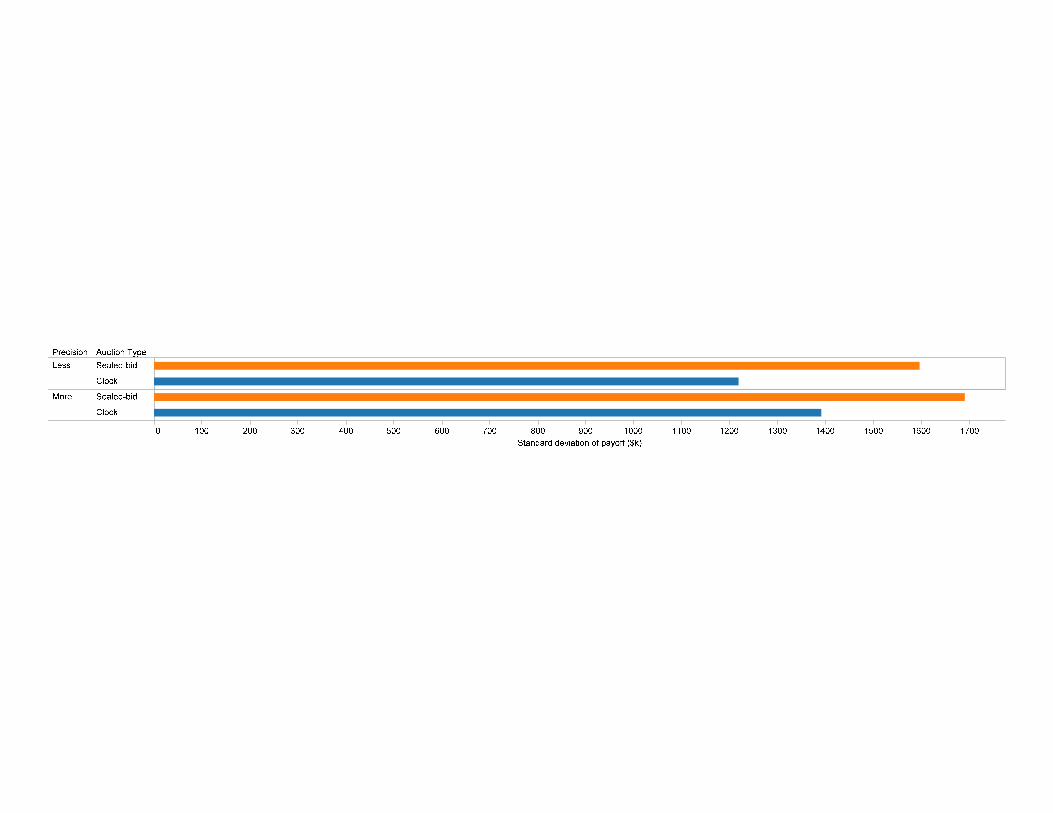
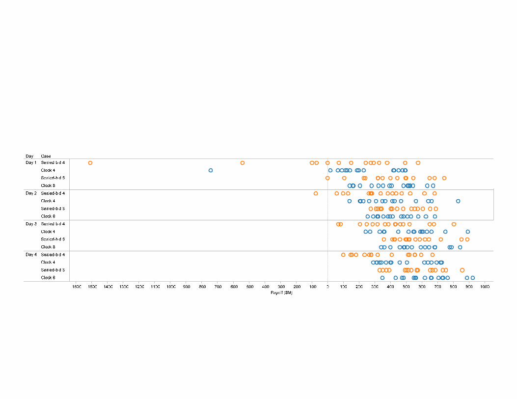
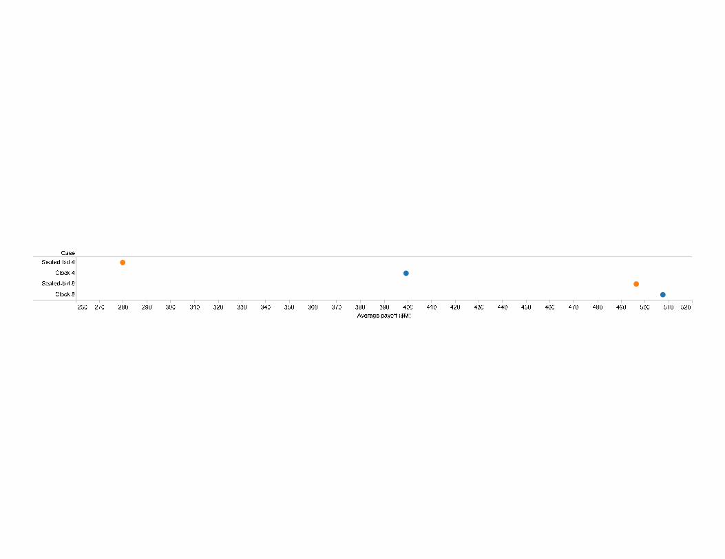
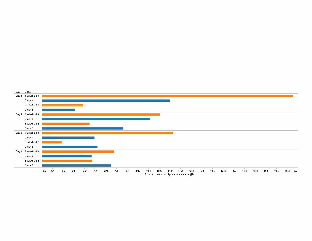
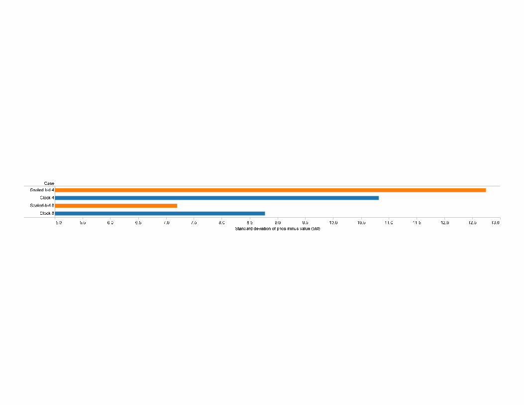
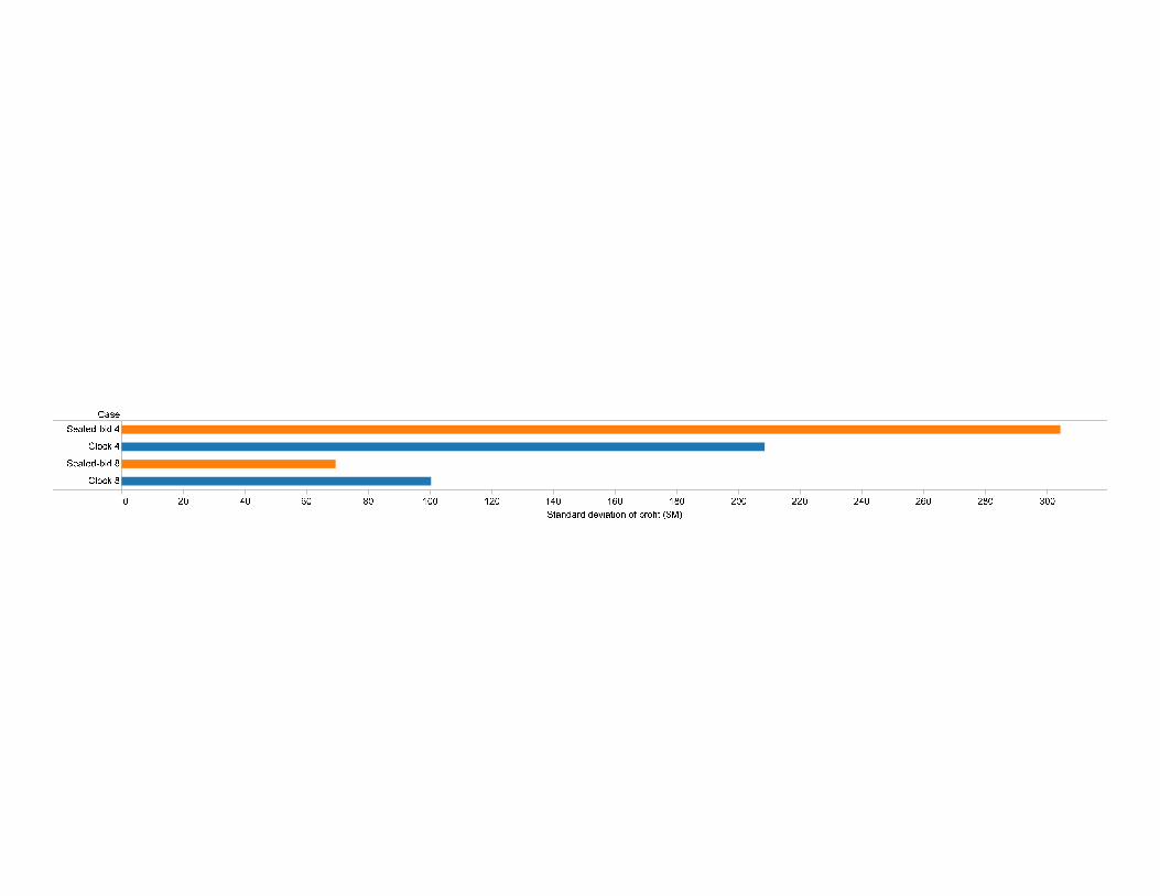
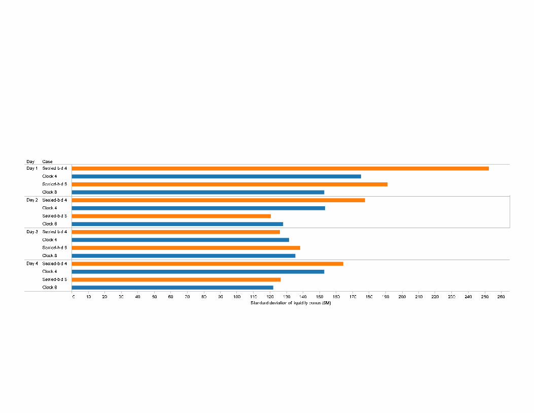
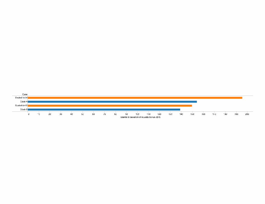
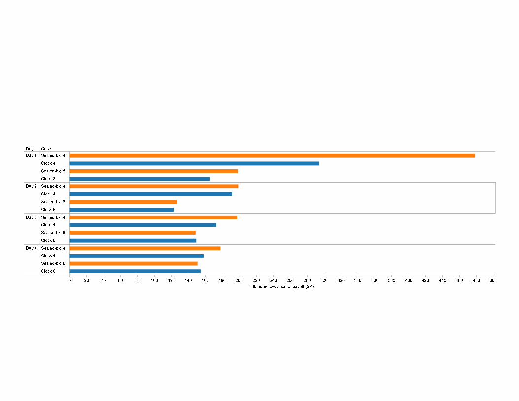
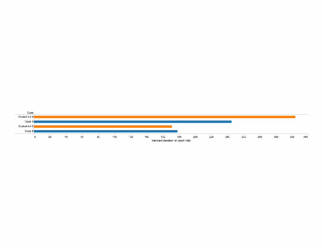
Sealed-bid vs. clock auction
• No difference in clearing priceg p
• Treasury buys securities at below true value, as banks seek cash
• Clock lets banks better manage liquidity needs
• Banks have higher payoff with clock
• Bank payoff is less variable with clock
Dynamic auction is win-win for banks and taxpayers
Pay
off

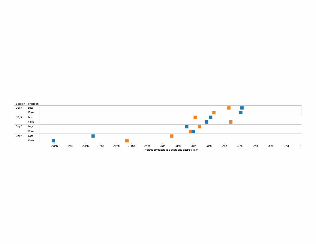
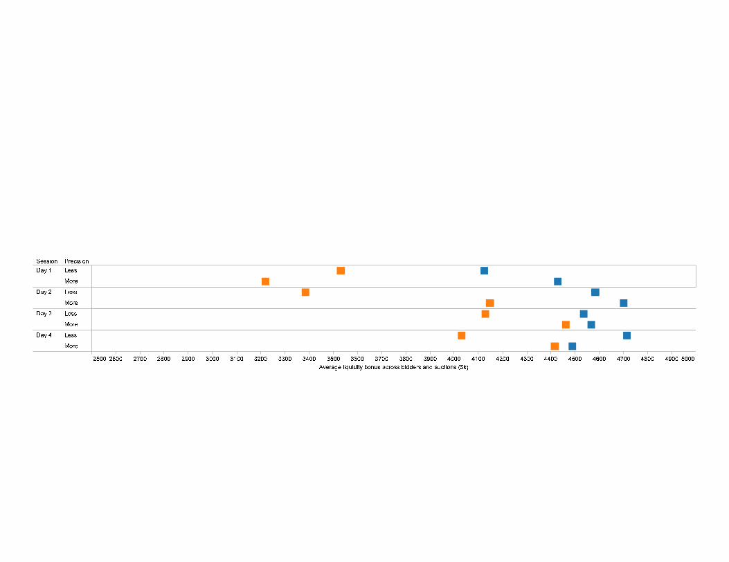

Session PrecisionDay 1 Less
More
Day 2 Less
More
Day 3 Less
More
Day 4 Less
2000 2200 2400 2600 2800 3000 3200 3400 3600 3800 4000 4200 4400 4600 4800 5000Average payoff across bidders and auctions ($k)
More


Less Precise
Less Precise
Less Precise
Less Precise
Less Precise
Less Precise
Less Precise

Less Precise
More Precise
More Precise
More Precise
More Precise
More Precise
More Precise
More Precise
More Precise

Experiment 1Experiment 1


4 bidder
4 bidder
4 bidder
4 bidder
4 bidder
4 bidder
4 bidder
4 bidder

4 bidder
4 bidder
4 bidder
4 bidder
4 bidder
4 bidder
4 bidder
4 bidder
8 bidder
8 bidder
8 bidder
8 bidder
8 bidder
8 bidder
8 bidder
8 bidder
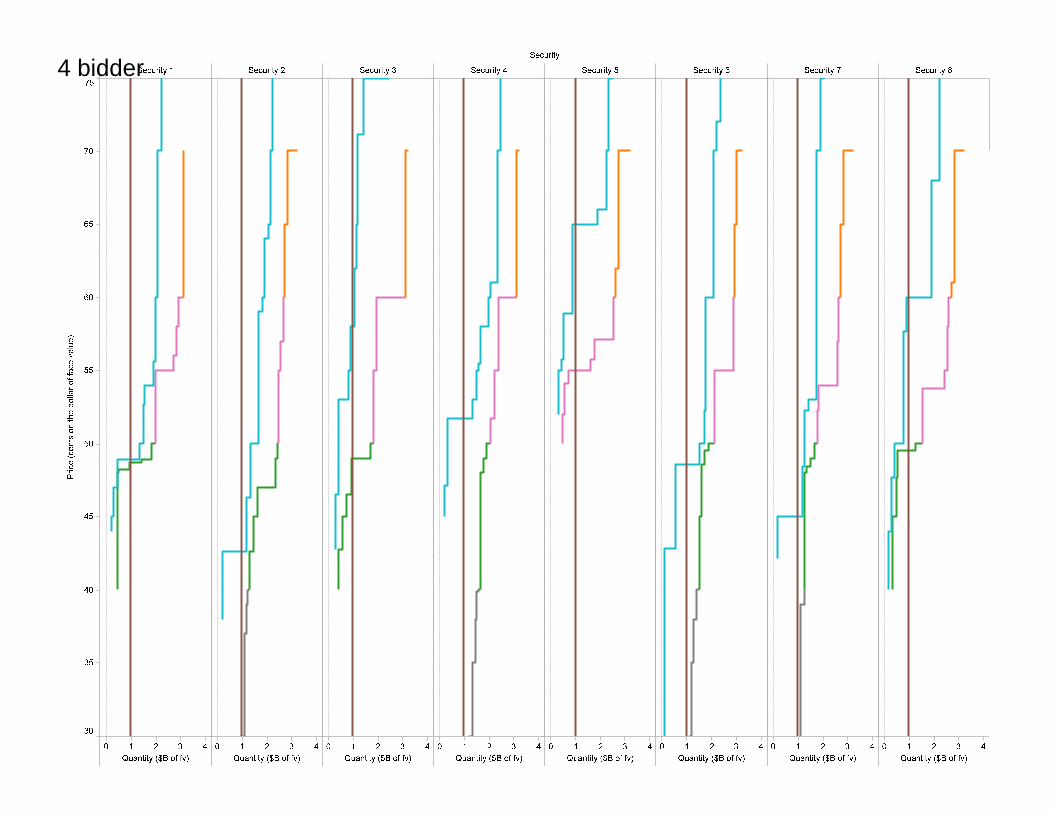
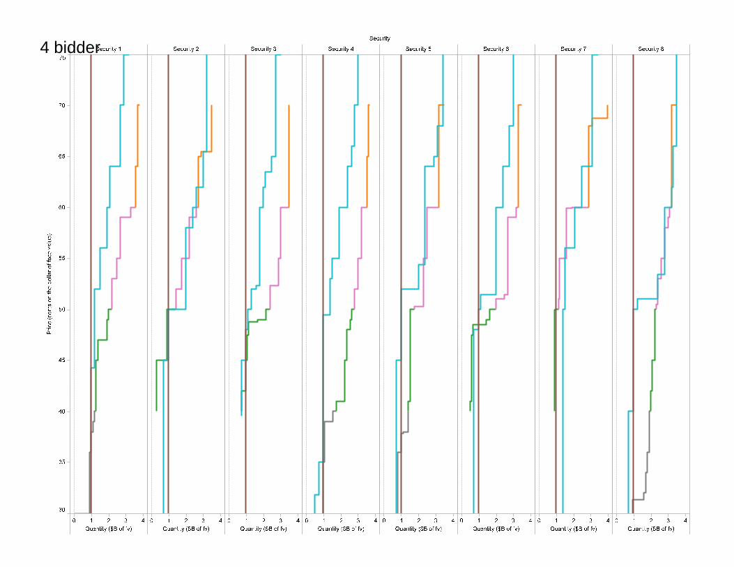
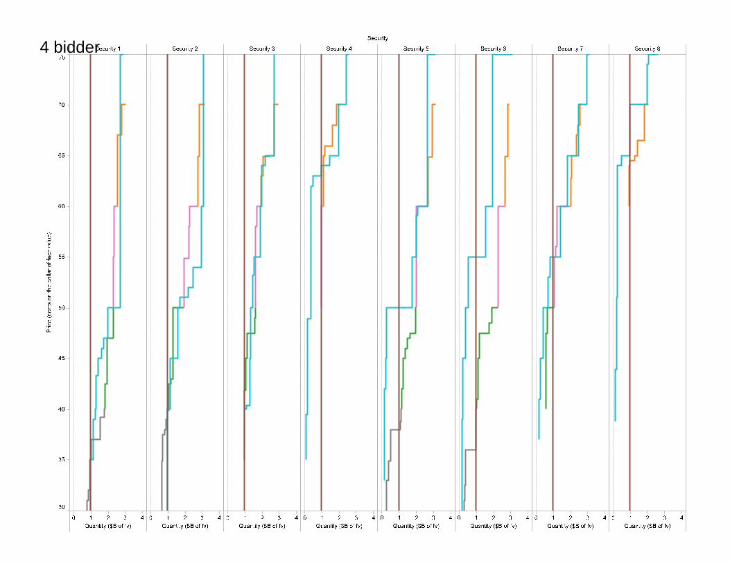
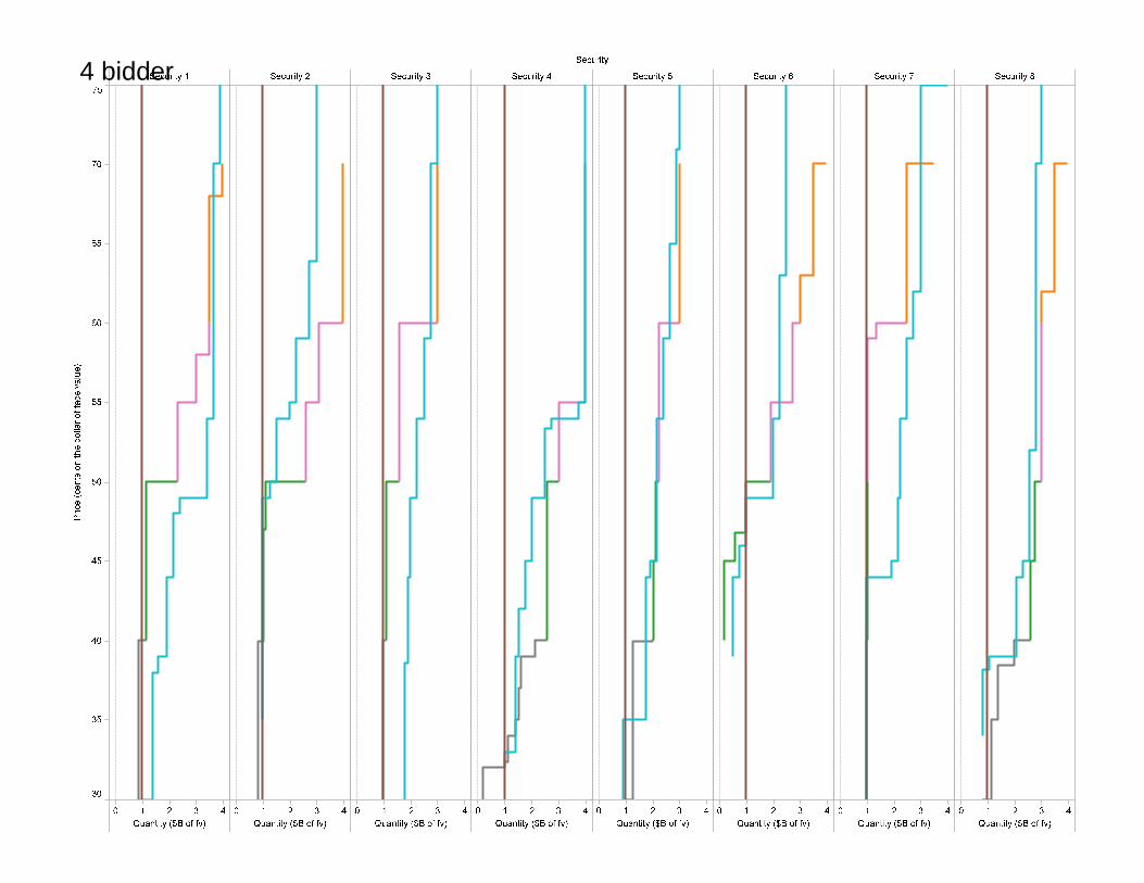
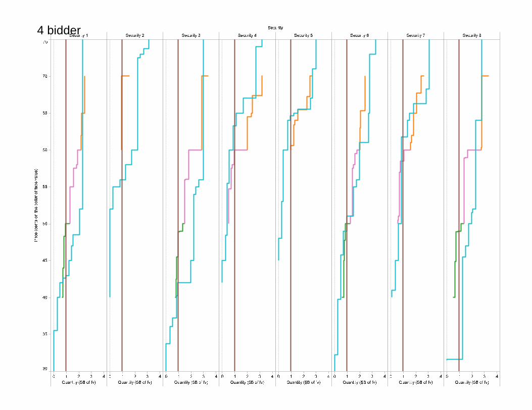
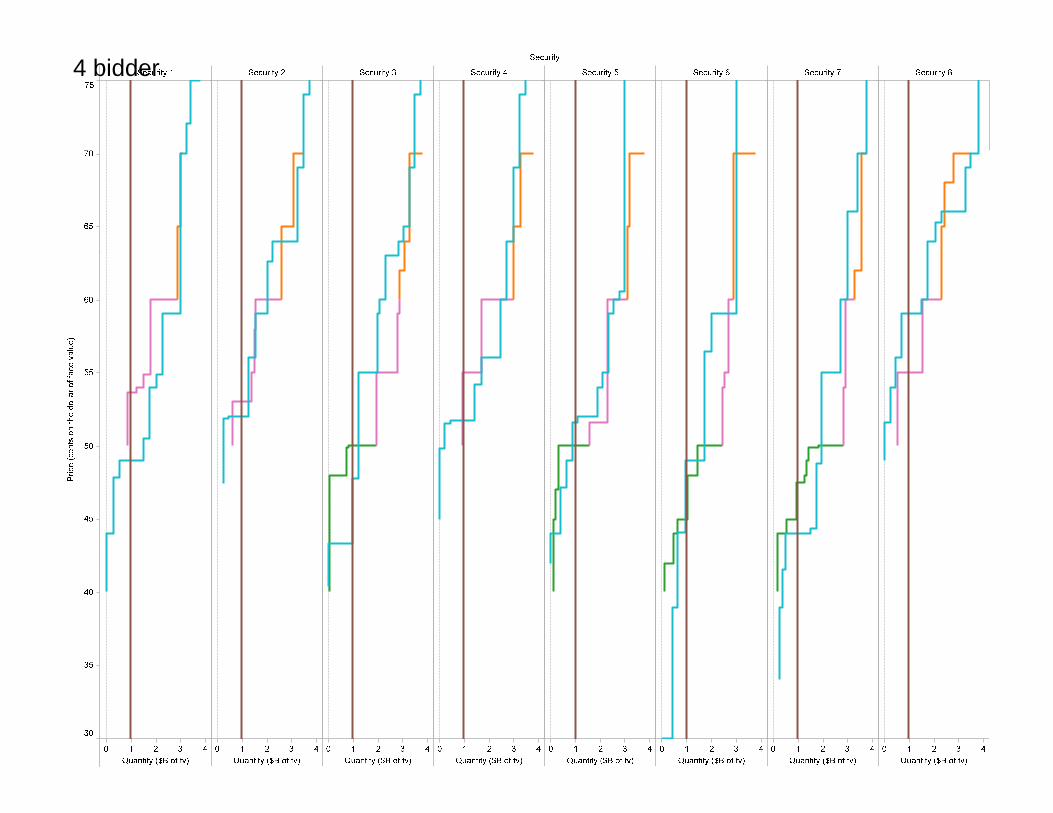
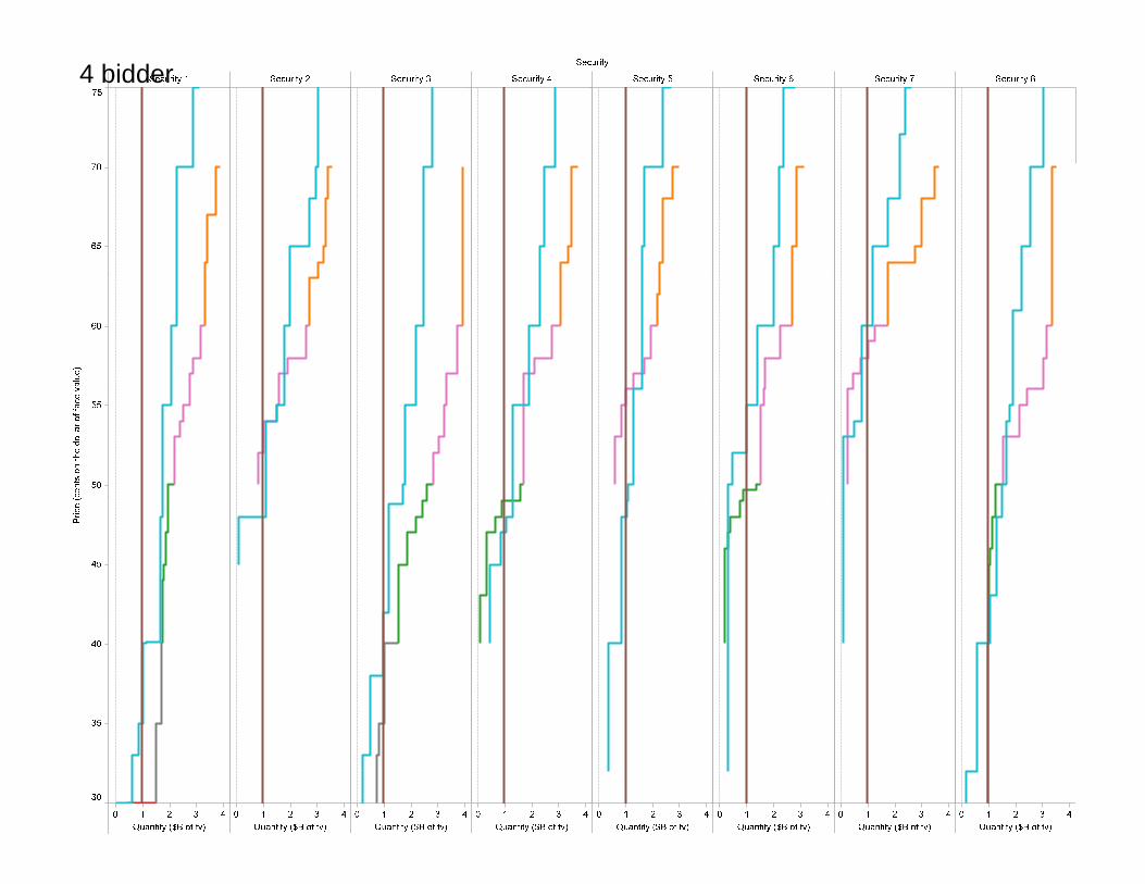
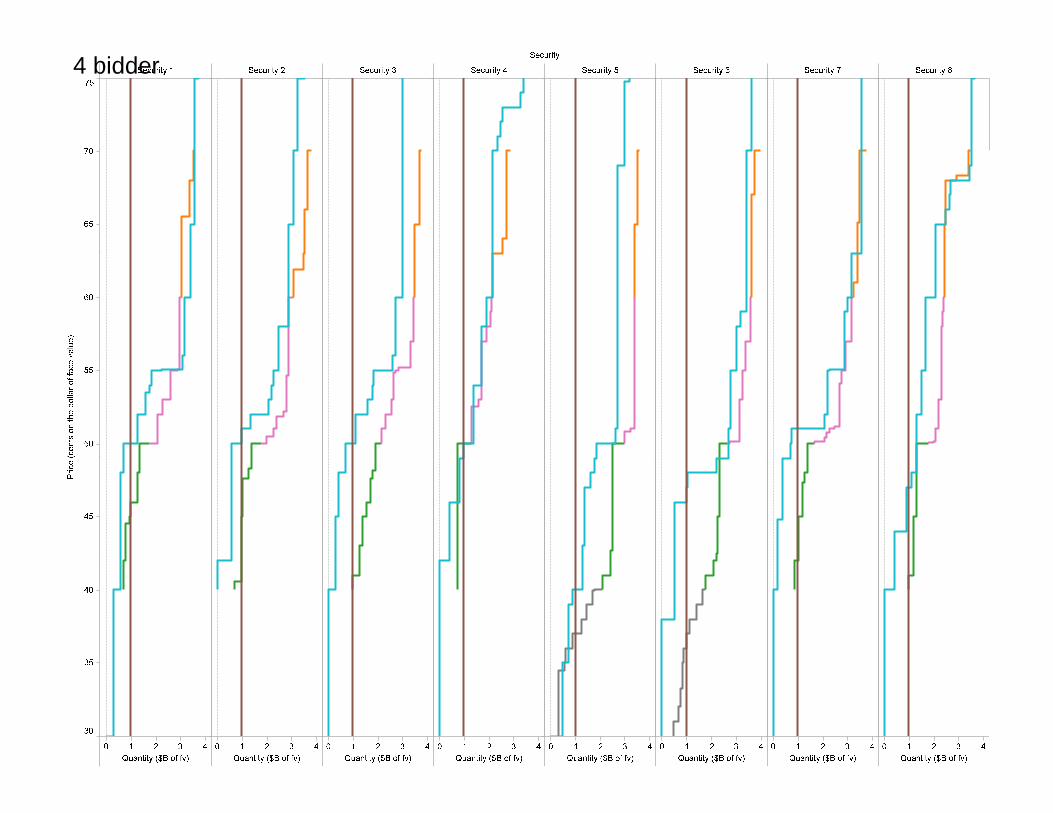
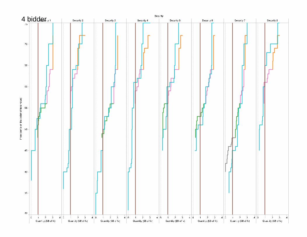
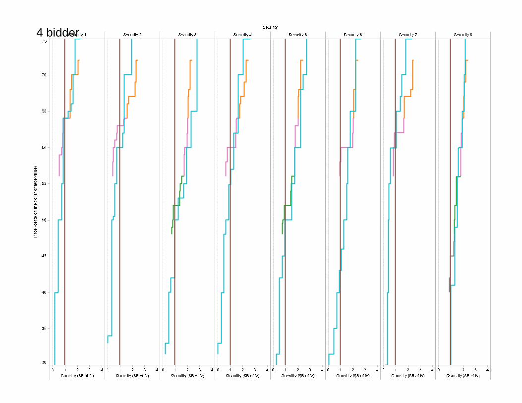
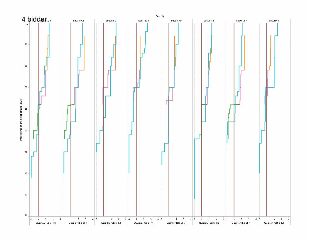
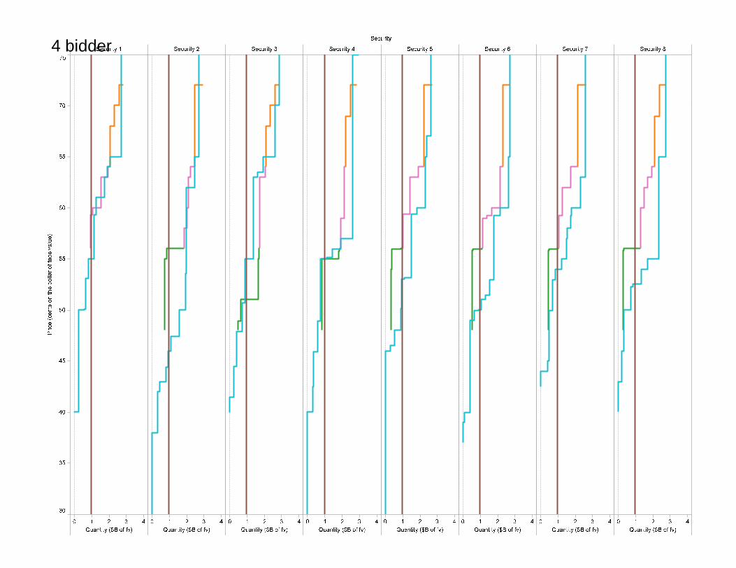
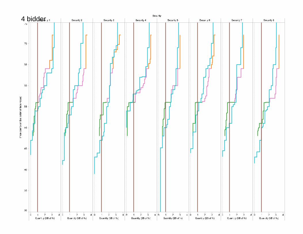
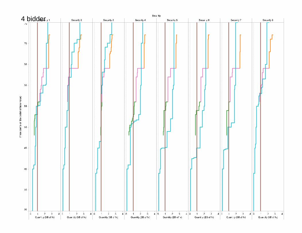
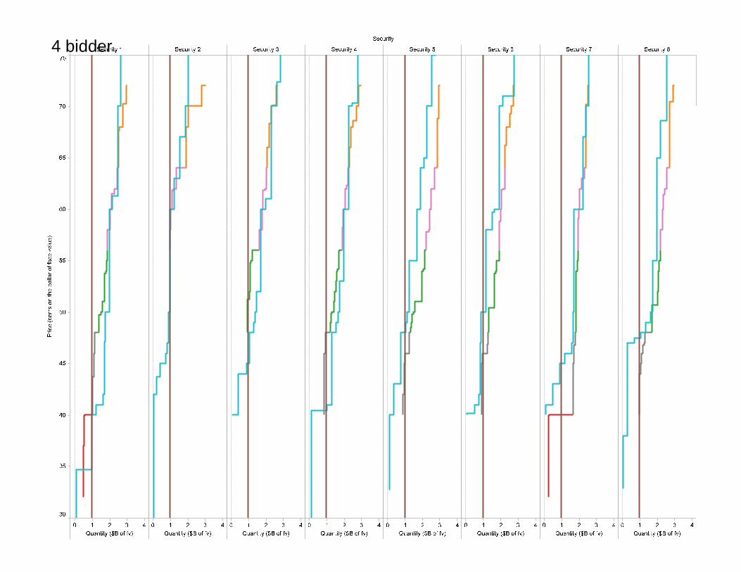
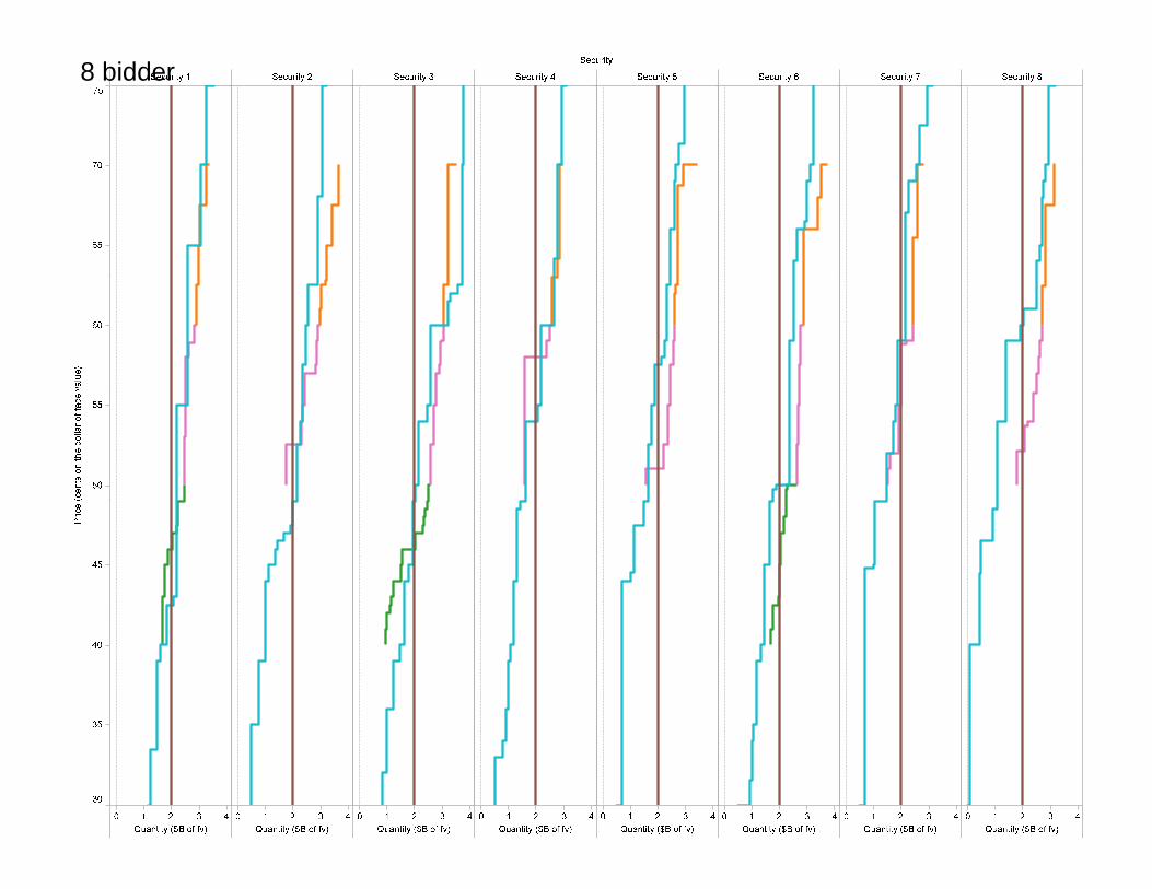
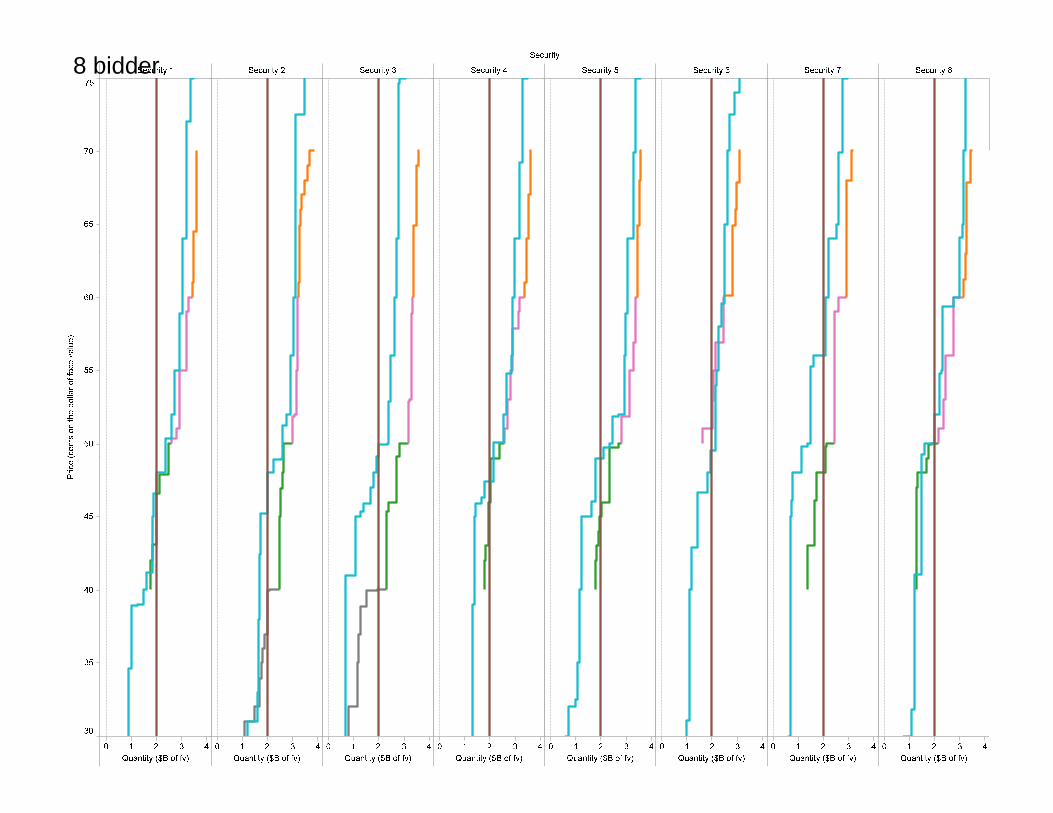
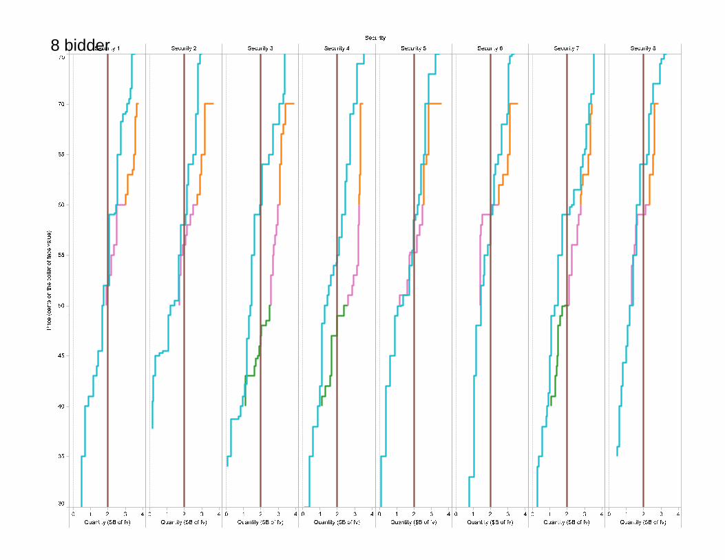
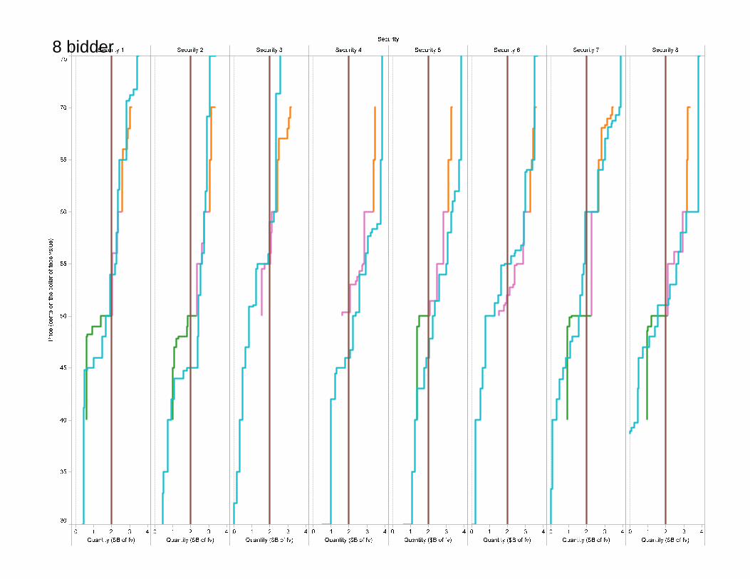
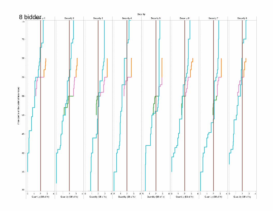
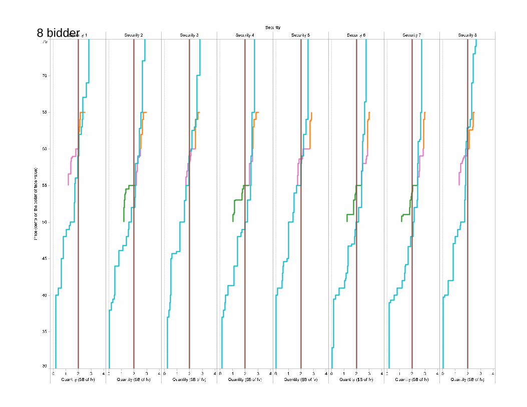
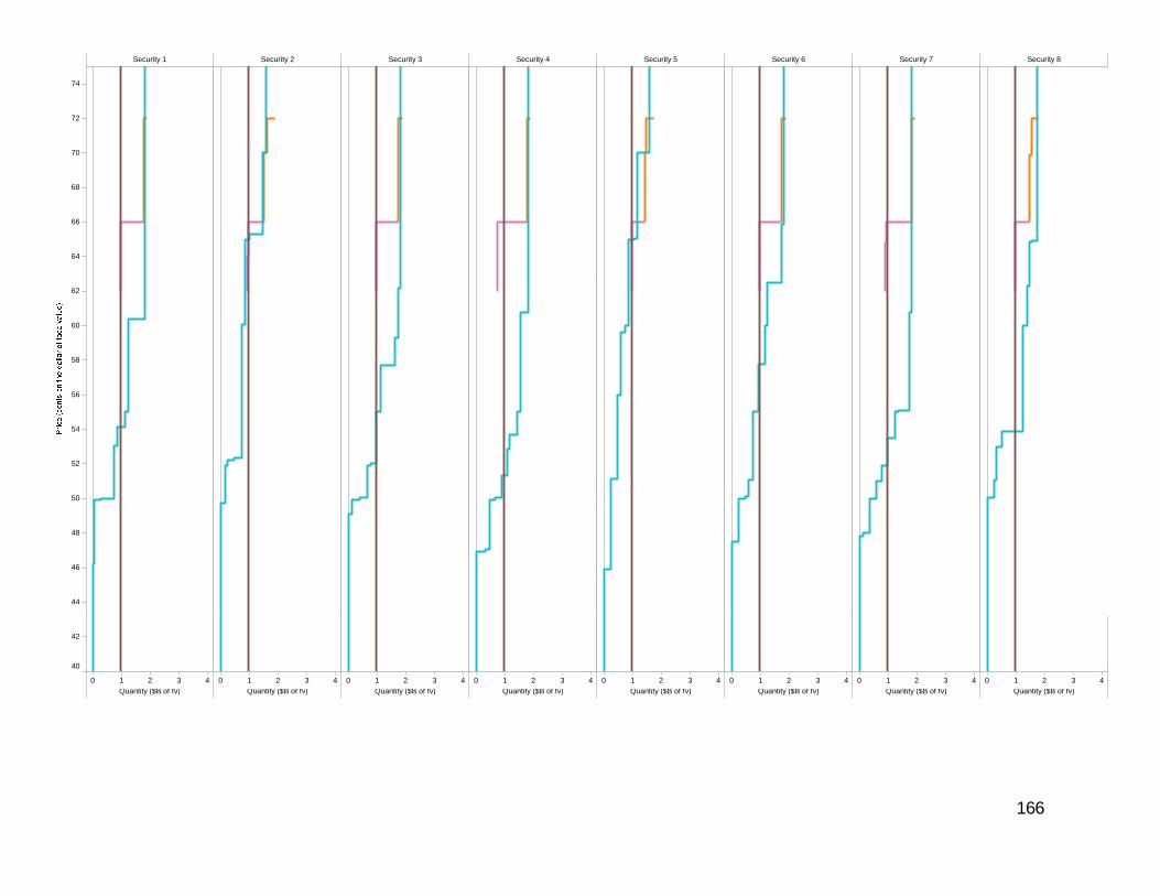
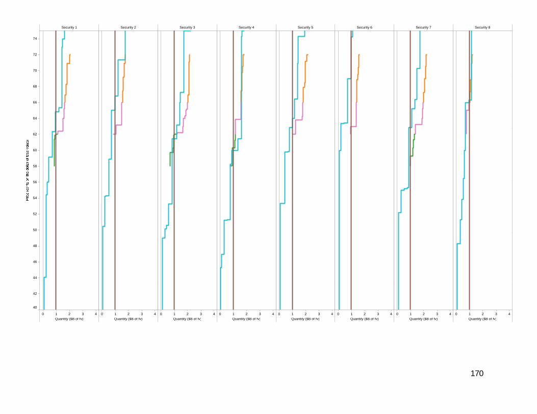
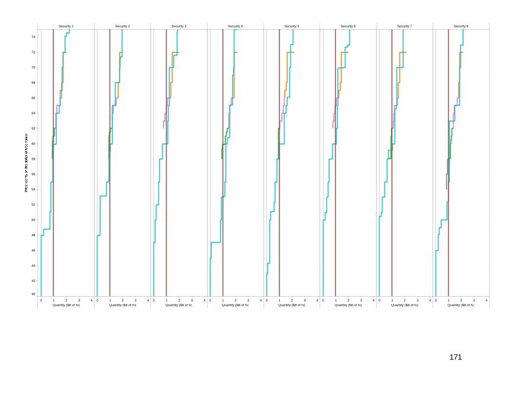
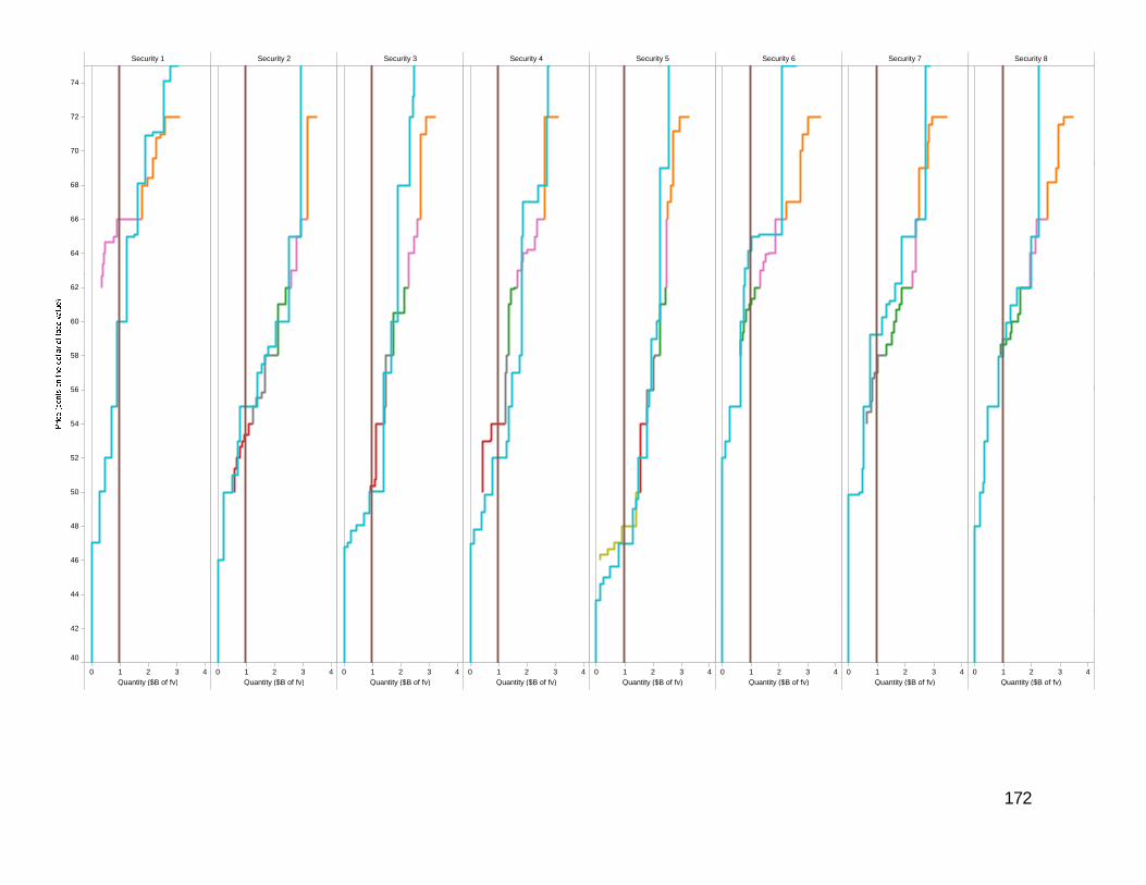
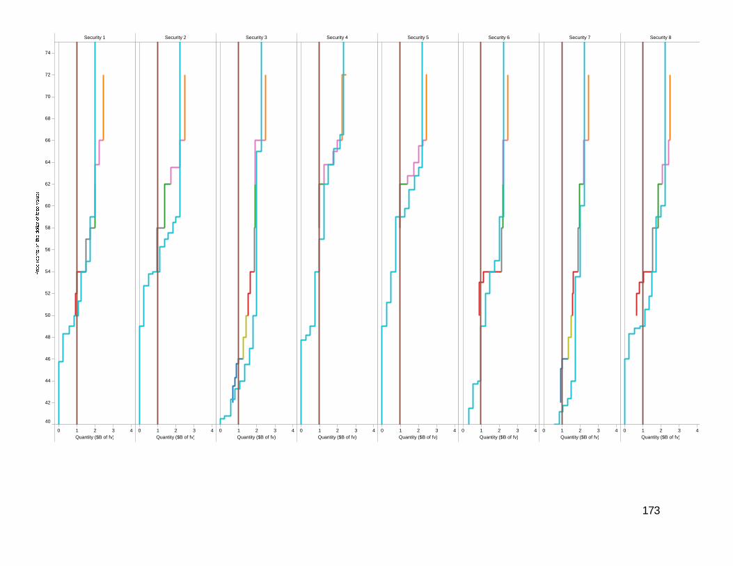
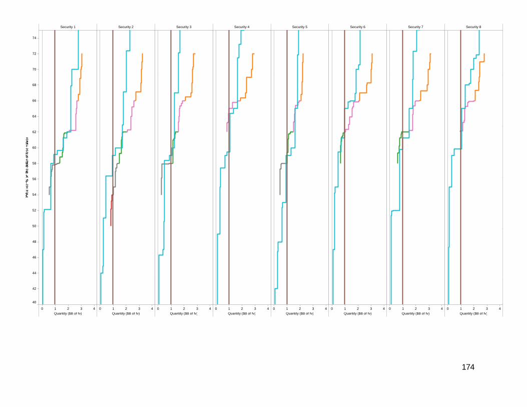
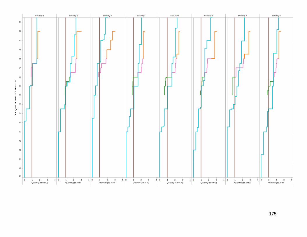
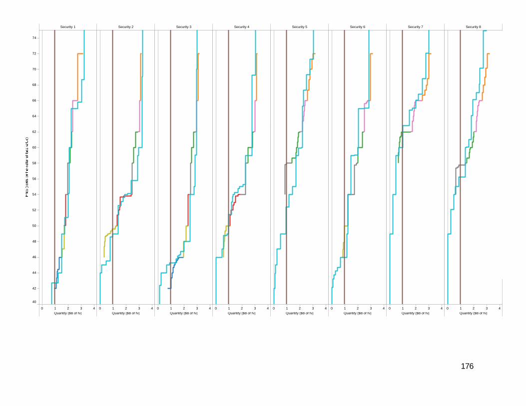
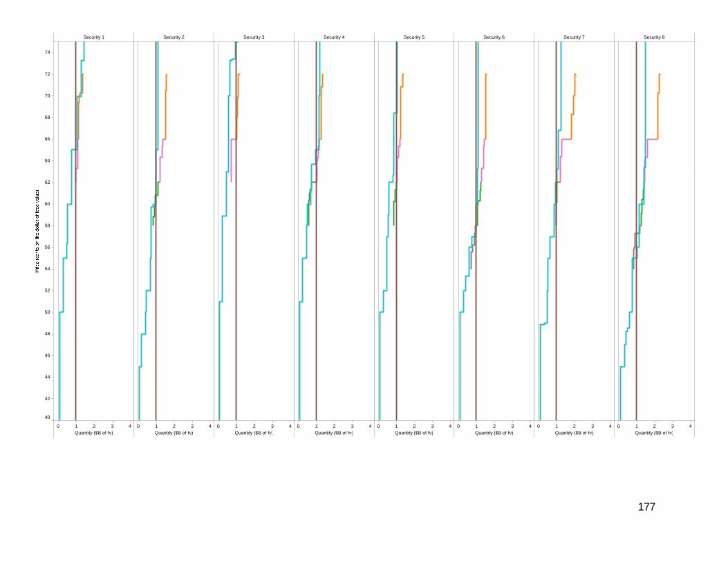
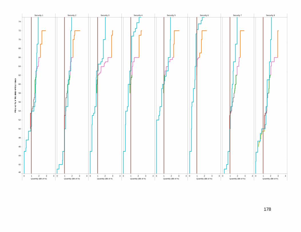
Experiment 3.1Security by SecuritySecurity by Security
No Liquidity Need4-bidder auctions
4 auctions per session2 i2 sessions
162
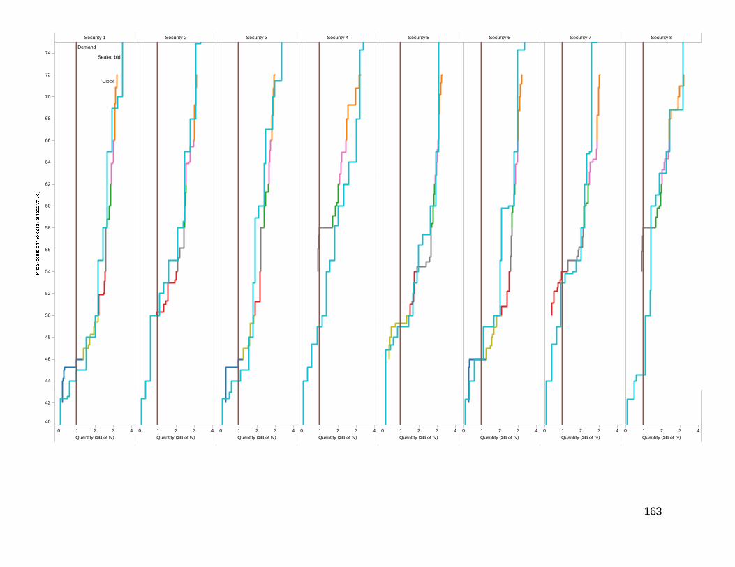
Security 1 Security 2 Security 3 Security 4 Security 5 Security 6 Security 7 Security 8
70
72
74Demand
Sealed bid
Clock
64
66
68
56
58
60
62
50
52
54
56
44
46
48
0 1 2 3 4Quantity ($B of fv)
0 1 2 3 4Quantity ($B of fv)
0 1 2 3 4Quantity ($B of fv)
0 1 2 3 4Quantity ($B of fv)
0 1 2 3 4Quantity ($B of fv)
0 1 2 3 4Quantity ($B of fv)
0 1 2 3 4Quantity ($B of fv)
0 1 2 3 4Quantity ($B of fv)
40
42
163
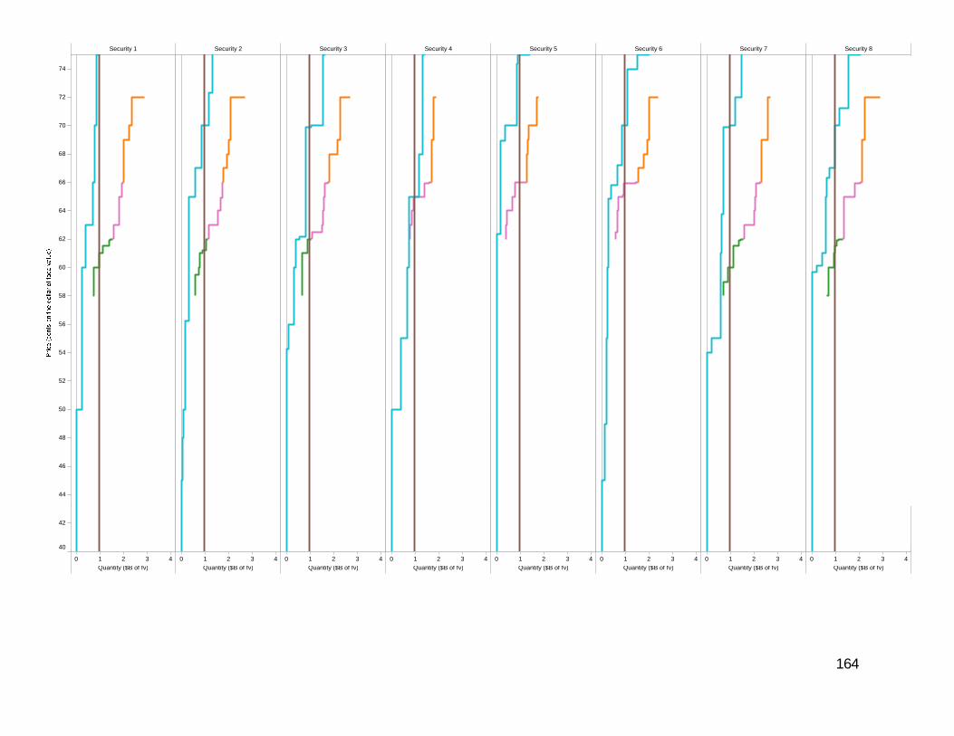
Security 1 Security 2 Security 3 Security 4 Security 5 Security 6 Security 7 Security 8
70
72
74
64
66
68
56
58
60
62
50
52
54
56
44
46
48
0 1 2 3 4Quantity ($B of fv)
0 1 2 3 4Quantity ($B of fv)
0 1 2 3 4Quantity ($B of fv)
0 1 2 3 4Quantity ($B of fv)
0 1 2 3 4Quantity ($B of fv)
0 1 2 3 4Quantity ($B of fv)
0 1 2 3 4Quantity ($B of fv)
0 1 2 3 4Quantity ($B of fv)
40
42
164
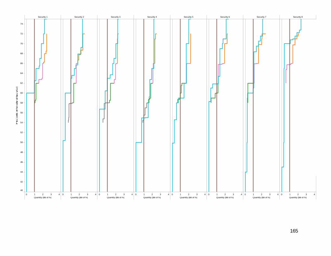
Security 1 Security 2 Security 3 Security 4 Security 5 Security 6 Security 7 Security 8
70
72
74
64
66
68
56
58
60
62
50
52
54
56
44
46
48
0 1 2 3 4Quantity ($B of fv)
0 1 2 3 4Quantity ($B of fv)
0 1 2 3 4Quantity ($B of fv)
0 1 2 3 4Quantity ($B of fv)
0 1 2 3 4Quantity ($B of fv)
0 1 2 3 4Quantity ($B of fv)
0 1 2 3 4Quantity ($B of fv)
0 1 2 3 4Quantity ($B of fv)
40
42
165
Security 1 Security 2 Security 3 Security 4 Security 5 Security 6 Security 7 Security 8
70
72
74
64
66
68
56
58
60
62
50
52
54
56
44
46
48
0 1 2 3 4Quantity ($B of fv)
0 1 2 3 4Quantity ($B of fv)
0 1 2 3 4Quantity ($B of fv)
0 1 2 3 4Quantity ($B of fv)
0 1 2 3 4Quantity ($B of fv)
0 1 2 3 4Quantity ($B of fv)
0 1 2 3 4Quantity ($B of fv)
0 1 2 3 4Quantity ($B of fv)
40
42
166

Security 1 Security 2 Security 3 Security 4 Security 5 Security 6 Security 7 Security 8
70
72
74
64
66
68
56
58
60
62
50
52
54
56
44
46
48
0 1 2 3 4Quantity ($B of fv)
0 1 2 3 4Quantity ($B of fv)
0 1 2 3 4Quantity ($B of fv)
0 1 2 3 4Quantity ($B of fv)
0 1 2 3 4Quantity ($B of fv)
0 1 2 3 4Quantity ($B of fv)
0 1 2 3 4Quantity ($B of fv)
0 1 2 3 4Quantity ($B of fv)
40
42
167

Security 1 Security 2 Security 3 Security 4 Security 5 Security 6 Security 7 Security 8
70
72
74
64
66
68
56
58
60
62
50
52
54
56
44
46
48
0 1 2 3 4Quantity ($B of fv)
0 1 2 3 4Quantity ($B of fv)
0 1 2 3 4Quantity ($B of fv)
0 1 2 3 4Quantity ($B of fv)
0 1 2 3 4Quantity ($B of fv)
0 1 2 3 4Quantity ($B of fv)
0 1 2 3 4Quantity ($B of fv)
0 1 2 3 4Quantity ($B of fv)
40
42
168

Security 1 Security 2 Security 3 Security 4 Security 5 Security 6 Security 7 Security 8
70
72
74
64
66
68
56
58
60
62
50
52
54
56
44
46
48
0 1 2 3 4Quantity ($B of fv)
0 1 2 3 4Quantity ($B of fv)
0 1 2 3 4Quantity ($B of fv)
0 1 2 3 4Quantity ($B of fv)
0 1 2 3 4Quantity ($B of fv)
0 1 2 3 4Quantity ($B of fv)
0 1 2 3 4Quantity ($B of fv)
0 1 2 3 4Quantity ($B of fv)
40
42
169
Security 1 Security 2 Security 3 Security 4 Security 5 Security 6 Security 7 Security 8
70
72
74
64
66
68
56
58
60
62
50
52
54
56
44
46
48
0 1 2 3 4Quantity ($B of fv)
0 1 2 3 4Quantity ($B of fv)
0 1 2 3 4Quantity ($B of fv)
0 1 2 3 4Quantity ($B of fv)
0 1 2 3 4Quantity ($B of fv)
0 1 2 3 4Quantity ($B of fv)
0 1 2 3 4Quantity ($B of fv)
0 1 2 3 4Quantity ($B of fv)
40
42
170
Security 1 Security 2 Security 3 Security 4 Security 5 Security 6 Security 7 Security 8
70
72
74
64
66
68
56
58
60
62
50
52
54
56
44
46
48
0 1 2 3 4Quantity ($B of fv)
0 1 2 3 4Quantity ($B of fv)
0 1 2 3 4Quantity ($B of fv)
0 1 2 3 4Quantity ($B of fv)
0 1 2 3 4Quantity ($B of fv)
0 1 2 3 4Quantity ($B of fv)
0 1 2 3 4Quantity ($B of fv)
0 1 2 3 4Quantity ($B of fv)
40
42
171
Security 1 Security 2 Security 3 Security 4 Security 5 Security 6 Security 7 Security 8
70
72
74
64
66
68
56
58
60
62
50
52
54
56
44
46
48
0 1 2 3 4Quantity ($B of fv)
0 1 2 3 4Quantity ($B of fv)
0 1 2 3 4Quantity ($B of fv)
0 1 2 3 4Quantity ($B of fv)
0 1 2 3 4Quantity ($B of fv)
0 1 2 3 4Quantity ($B of fv)
0 1 2 3 4Quantity ($B of fv)
0 1 2 3 4Quantity ($B of fv)
40
42
172
Security 1 Security 2 Security 3 Security 4 Security 5 Security 6 Security 7 Security 8
70
72
74
64
66
68
58
60
62
50
52
54
56
44
46
48
0 1 2 3 4Quantity ($B of fv)
0 1 2 3 4Quantity ($B of fv)
0 1 2 3 4Quantity ($B of fv)
0 1 2 3 4Quantity ($B of fv)
0 1 2 3 4Quantity ($B of fv)
0 1 2 3 4Quantity ($B of fv)
0 1 2 3 4Quantity ($B of fv)
0 1 2 3 4Quantity ($B of fv)
40
42
173
Security 1 Security 2 Security 3 Security 4 Security 5 Security 6 Security 7 Security 8
70
72
74
64
66
68
56
58
60
62
50
52
54
56
44
46
48
0 1 2 3 4Quantity ($B of fv)
0 1 2 3 4Quantity ($B of fv)
0 1 2 3 4Quantity ($B of fv)
0 1 2 3 4Quantity ($B of fv)
0 1 2 3 4Quantity ($B of fv)
0 1 2 3 4Quantity ($B of fv)
0 1 2 3 4Quantity ($B of fv)
0 1 2 3 4Quantity ($B of fv)
40
42
174
Security 1 Security 2 Security 3 Security 4 Security 5 Security 6 Security 7 Security 8
70
72
74
64
66
68
56
58
60
62
50
52
54
56
44
46
48
0 1 2 3 4Quantity ($B of fv)
0 1 2 3 4Quantity ($B of fv)
0 1 2 3 4Quantity ($B of fv)
0 1 2 3 4Quantity ($B of fv)
0 1 2 3 4Quantity ($B of fv)
0 1 2 3 4Quantity ($B of fv)
0 1 2 3 4Quantity ($B of fv)
0 1 2 3 4Quantity ($B of fv)
40
42
175
Security 1 Security 2 Security 3 Security 4 Security 5 Security 6 Security 7 Security 8
70
72
74
64
66
68
56
58
60
62
50
52
54
56
44
46
48
0 1 2 3 4Quantity ($B of fv)
0 1 2 3 4Quantity ($B of fv)
0 1 2 3 4Quantity ($B of fv)
0 1 2 3 4Quantity ($B of fv)
0 1 2 3 4Quantity ($B of fv)
0 1 2 3 4Quantity ($B of fv)
0 1 2 3 4Quantity ($B of fv)
0 1 2 3 4Quantity ($B of fv)
40
42
176
Security 1 Security 2 Security 3 Security 4 Security 5 Security 6 Security 7 Security 8
70
72
74
64
66
68
56
58
60
62
50
52
54
56
44
46
48
0 1 2 3 4Quantity ($B of fv)
0 1 2 3 4Quantity ($B of fv)
0 1 2 3 4Quantity ($B of fv)
0 1 2 3 4Quantity ($B of fv)
0 1 2 3 4Quantity ($B of fv)
0 1 2 3 4Quantity ($B of fv)
0 1 2 3 4Quantity ($B of fv)
0 1 2 3 4Quantity ($B of fv)
40
42
177
Security 1 Security 2 Security 3 Security 4 Security 5 Security 6 Security 7 Security 8
70
72
74
64
66
68
56
58
60
62
50
52
54
56
44
46
48
0 1 2 3 4Quantity ($B of fv)
0 1 2 3 4Quantity ($B of fv)
0 1 2 3 4Quantity ($B of fv)
0 1 2 3 4Quantity ($B of fv)
0 1 2 3 4Quantity ($B of fv)
0 1 2 3 4Quantity ($B of fv)
0 1 2 3 4Quantity ($B of fv)
0 1 2 3 4Quantity ($B of fv)
40
42
178
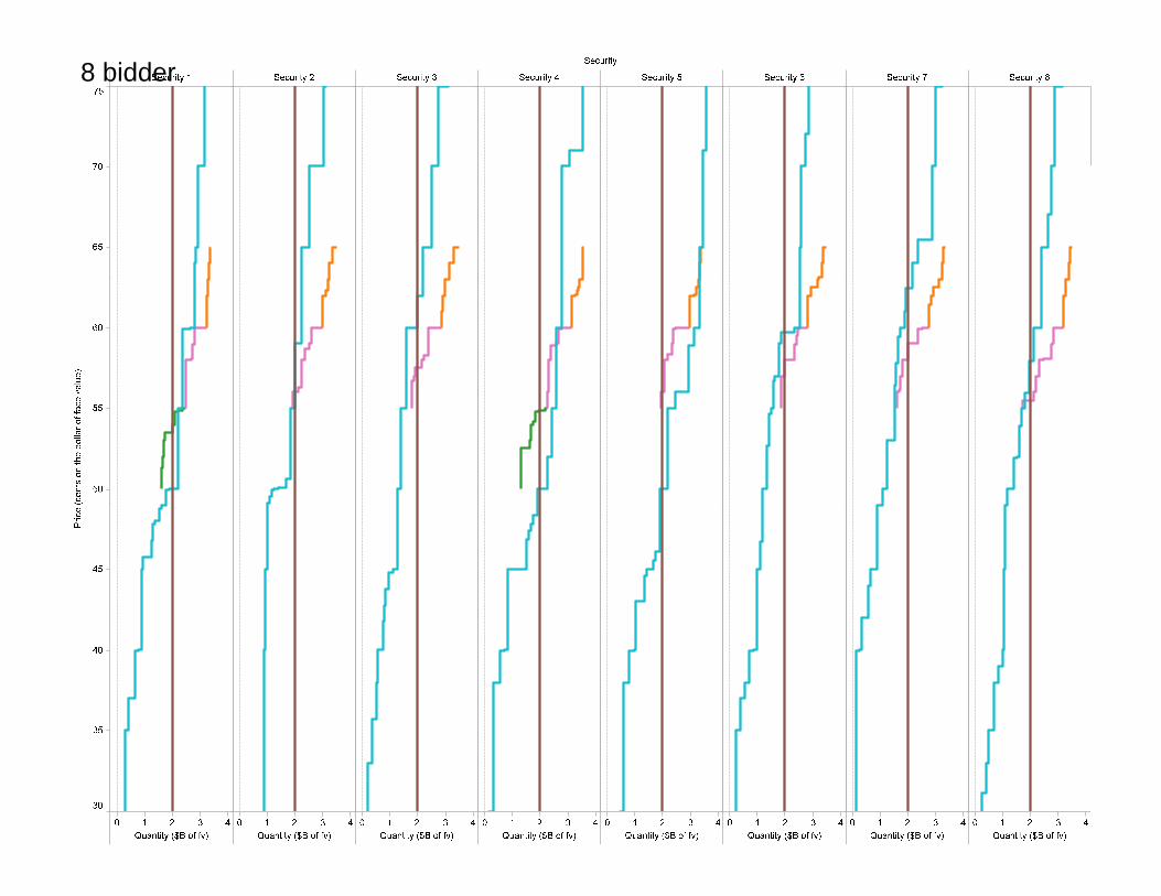
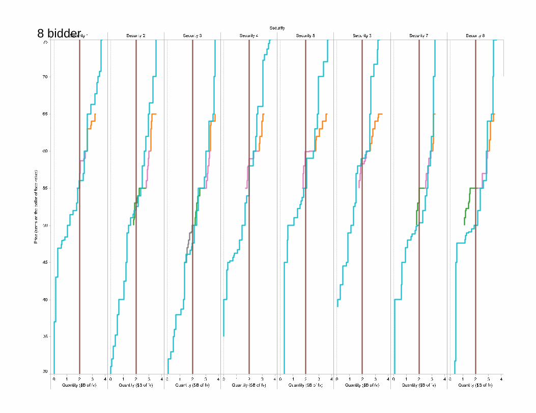
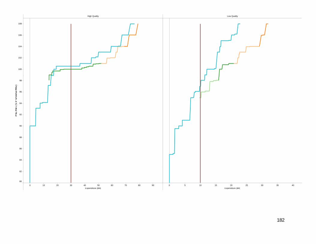
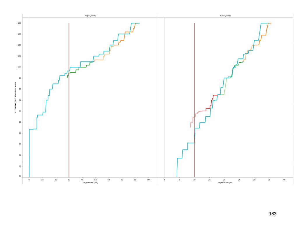
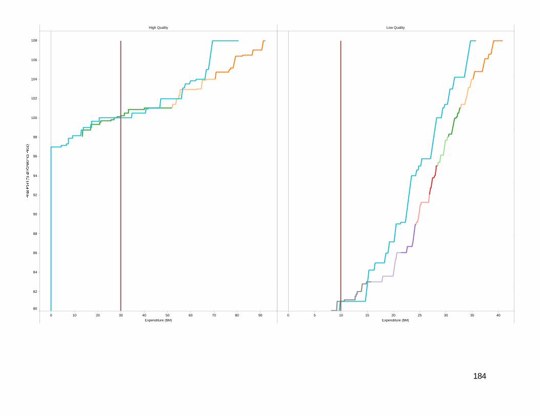
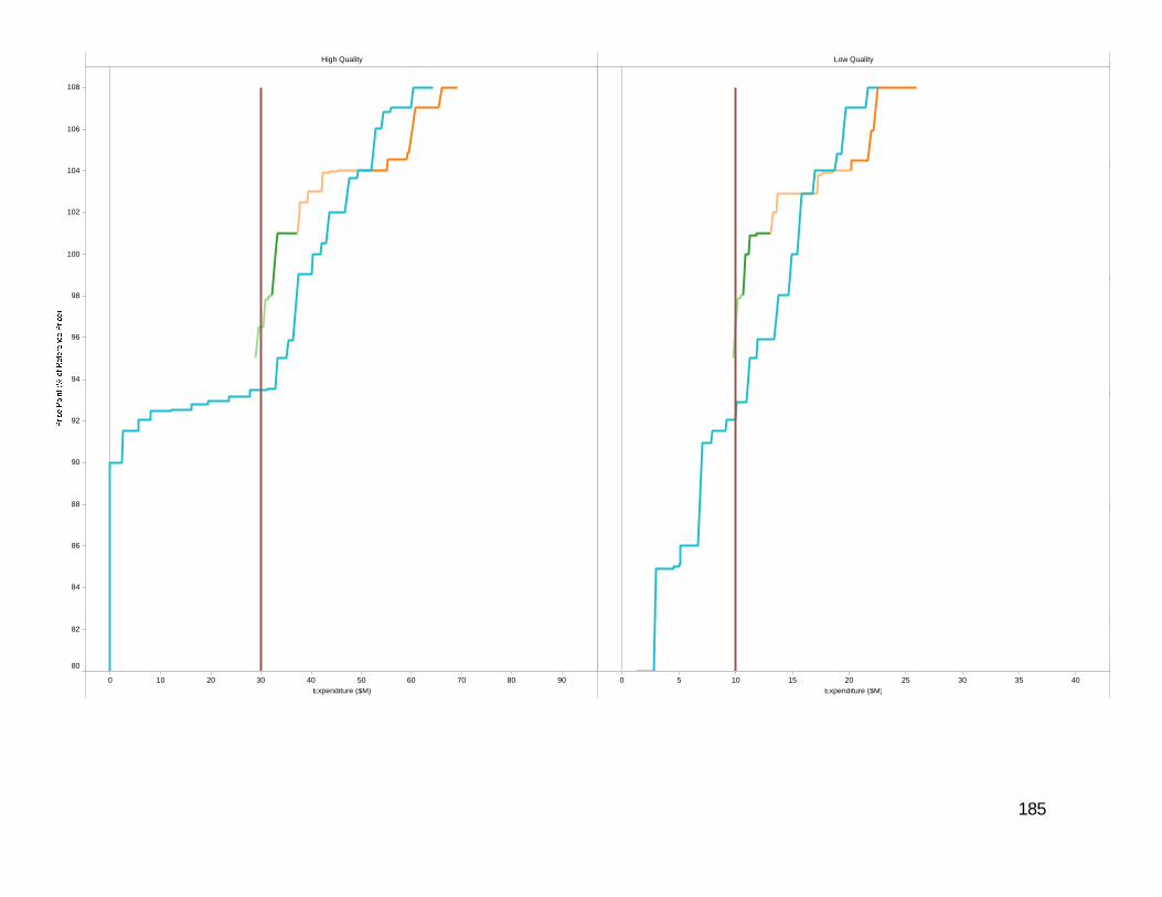
Experiment 3.2Reference PriceReference Price
No Liquidity Need8-bidder auctions
4 auctions per session2 i2 sessions
179
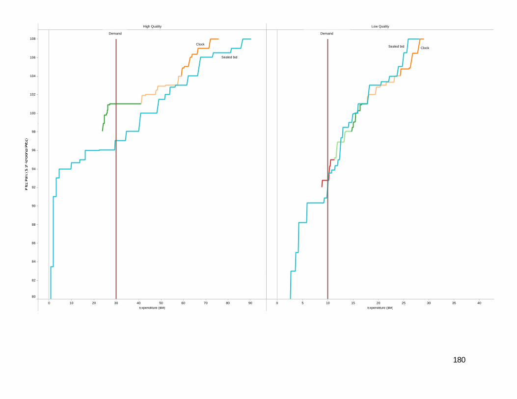
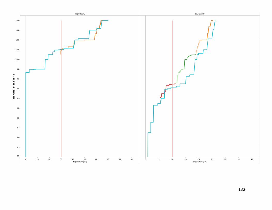
High Quality Low Quality
106
108Demand Demand
Clock
Sealed bid
Sealed bid Clock
100
102
104
94
96
98
88
90
92
84
86
88
0 10 20 30 40 50 60 70 80 90Expenditure ($M)
0 5 10 15 20 25 30 35 40Expenditure ($M)
80
82
180

High Quality Low Quality
106
108
100
102
104
94
96
98
88
90
92
84
86
88
0 10 20 30 40 50 60 70 80 90Expenditure ($M)
0 5 10 15 20 25 30 35 40Expenditure ($M)
80
82
181
High Quality Low Quality
106
108
100
102
104
94
96
98
88
90
92
84
86
88
0 10 20 30 40 50 60 70 80 90Expenditure ($M)
0 5 10 15 20 25 30 35 40Expenditure ($M)
80
82
182
High Quality Low Quality
106
108
100
102
104
94
96
98
88
90
92
84
86
88
0 10 20 30 40 50 60 70 80 90Expenditure ($M)
0 5 10 15 20 25 30 35 40Expenditure ($M)
80
82
183
High Quality Low Quality
106
108
100
102
104
94
96
98
88
90
92
84
86
0 10 20 30 40 50 60 70 80 90Expenditure ($M)
0 5 10 15 20 25 30 35 40Expenditure ($M)
80
82
184
High Quality Low Quality
106
108
100
102
104
94
96
98
88
90
92
84
86
88
0 10 20 30 40 50 60 70 80 90Expenditure ($M)
0 5 10 15 20 25 30 35 40Expenditure ($M)
80
82
185
High Quality Low Quality
106
108
100
102
104
94
96
98
88
90
92
84
86
88
0 10 20 30 40 50 60 70 80 90Expenditure ($M)
0 5 10 15 20 25 30 35 40Expenditure ($M)
80
82
186
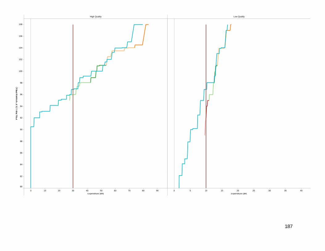
High Quality Low Quality
106
108
100
102
104
94
96
98
88
90
92
84
86
88
0 10 20 30 40 50 60 70 80 90Expenditure ($M)
0 5 10 15 20 25 30 35 40Expenditure ($M)
80
82
187
payo
ff
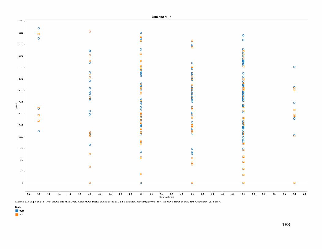
188
payo
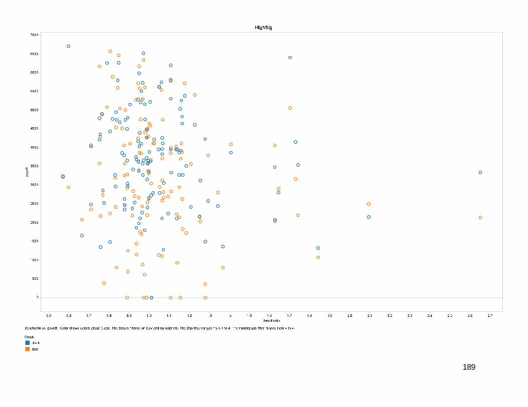
ff
189
payo
ff
190

payo
ff
191
of tt
lpro
fitSu
m
Avg.
pay
off
192
. ttlp
rofit
Avg
yoff
Avg.
pay
193
194
vg. p
ayof
fA
vA
vg. t
tlpro
fit
195
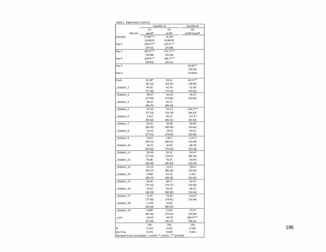
Table 1. Experiment 1 (and 3)Liquidity=0
(1) (2) (3)dep var: payoff profit profit=payoff
Liquidity 0.740*** ‐0.159[0.0912] [0.0879]
Day 2 183.4*** 123.9***[ ] [ ]
Liquidity >0
[37.01] [35.68]Day 3 283.9*** 211.7***
[36.88] [35.56]Day 4 250.0*** 184.3***
[36.83] [35.51]Day 5 58.82**
[19.59]Day 6 omitted
Clock 65.39* 26.51 60.13**[25.22] [24.31] [18.96]
_ISubject_2 45.02 42.74 ‐22.30[77.48] [74.70] [53.64]
_ISubject_3 ‐99.67 ‐43.34 ‐45.37[77.40] [74.62] [53.64]
_ISubject_4 38.14 42.71[83.35] [80.36]
ISubject 5 ‐67.36 ‐53.21 ‐239.2***_ j _[77.53] [74.74] [66.42]
_ISubject_6 2.353 60.12 ‐127.6*[83.30] [80.31] [53.64]
_ISubject_7 50.32 50.68 ‐60.40[83.26] [80.28] [53.64]
_ISubject_8 ‐16.25 ‐18.32 ‐64.31[77.41] [74.63] [53.64]
_ISubject_9 115.0 126.7 ‐113.5*[83 51] [80 51] [53 64][83.51] [80.51] [53.64]
_ISubject_10 ‐16.25 ‐4.615 ‐86.78[82.46] [79.50] [53.64]
_ISubject_11 ‐20.59 32.51 ‐53.47[77.45] [74.67] [66.42]
_ISubject_12 93.86 70.37 ‐59.59[83.38] [80.39] [53.64]
_ISubject_13 ‐91.53 ‐114.2 ‐101.0[83.27] [80.28] [53.64]
ISubject 14 2 848 61 25 5 287_ISubject_14 2.848 61.25 5.287[83.27] [80.28] [53.64]
_ISubject_15 56.64 68.17 ‐62.47[77.55] [74.77] [53.64]
_ISubject_16 19.63 64.14 ‐66.53[83.29] [80.30] [53.64]
_ISubject_17 71.97 79.94 ‐116.6*[77.60] [74.81] [53.64]
_ISubject_18 ‐3.744 16.03
196
[83.50] [80.50]_ISubject_19 4.689 3.245 ‐73.27
[82.36] [79.41] [53.64]_cons ‐24.62 ‐64.70 280.2***
[87.89] [84.73] [48.41]256 256 128
N 0.374 0.142 0.196adj. R‐sq 0.374 0.018 0.341Standard errors in brackets; * p<0.05 ** p<0.01 *** p<0.001
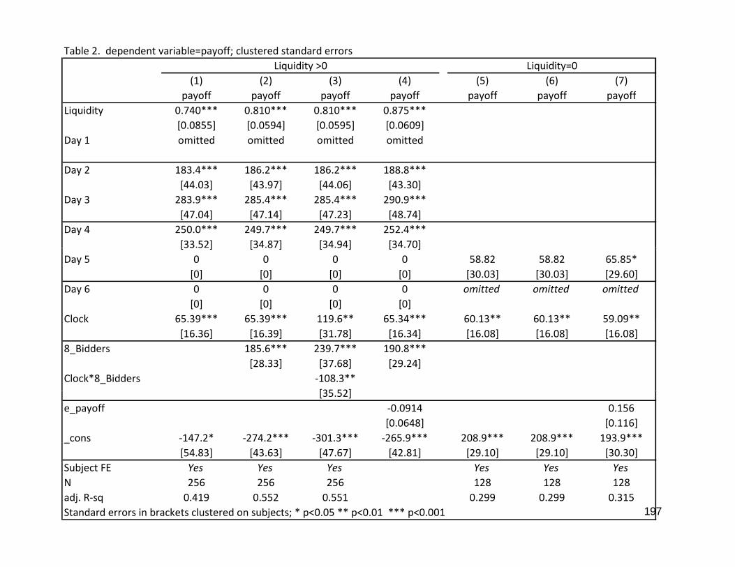
Table 2. dependent variable=payoff; clustered standard errors
(1) (2) (3) (4) (5) (6) (7)payoff payoff payoff payoff payoff payoff payoff
Liquidity=0Liquidity >0
Liquidity 0.740*** 0.810*** 0.810*** 0.875***[0.0855] [0.0594] [0.0595] [0.0609]
Day 1 omitted omitted omitted omitted
Day 2 183.4*** 186.2*** 186.2*** 188.8***[44.03] [43.97] [44.06] [43.30]
Day 3 283.9*** 285.4*** 285.4*** 290.9***[47.04] [47.14] [47.23] [48.74]
Day 4 250.0*** 249.7*** 249.7*** 252.4***[33.52] [34.87] [34.94] [34.70][33 5 ] [3 8 ] [3 9 ] [3 0]
Day 5 0 0 0 0 58.82 58.82 65.85*[0] [0] [0] [0] [30.03] [30.03] [29.60]
Day 6 0 0 0 0 omitted omitted omitted[0] [0] [0] [0]
Clock 65 39*** 65 39*** 119 6** 65 34*** 60 13** 60 13** 59 09**Clock 65.39 65.39 119.6 65.34 60.13 60.13 59.09[16.36] [16.39] [31.78] [16.34] [16.08] [16.08] [16.08]
8_Bidders 185.6*** 239.7*** 190.8***[28.33] [37.68] [29.24]
Clock*8_Bidders ‐108.3**[35 52][35.52]
e_payoff ‐0.0914 0.156[0.0648] [0.116]
_cons ‐147.2* ‐274.2*** ‐301.3*** ‐265.9*** 208.9*** 208.9*** 193.9***[54.83] [43.63] [47.67] [42.81] [29.10] [29.10] [30.30]
197
Subject FE Yes Yes Yes Yes Yes YesN 256 256 256 128 128 128adj. R‐sq 0.419 0.552 0.551 0.299 0.299 0.315Standard errors in brackets clustered on subjects; * p<0.05 ** p<0.01 *** p<0.001
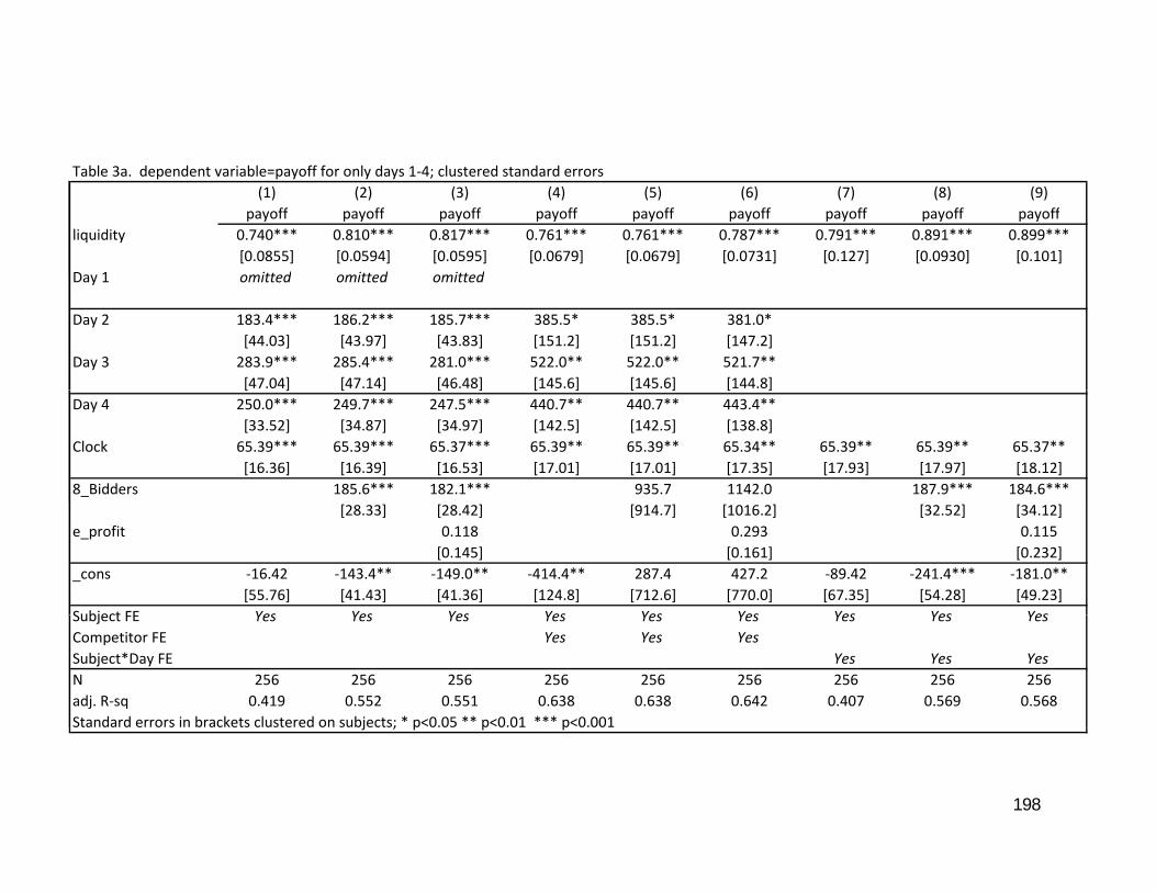
Table 3a. dependent variable=payoff for only days 1‐4; clustered standard errors(1) (2) (3) (4) (5) (6) (7) (8) (9)
payoff payoff payoff payoff payoff payoff payoff payoff payoffliquidity 0.740*** 0.810*** 0.817*** 0.761*** 0.761*** 0.787*** 0.791*** 0.891*** 0.899***
[0.0855] [0.0594] [0.0595] [0.0679] [0.0679] [0.0731] [0.127] [0.0930] [0.101]Day 1 omitted omitted omittedDay 1 omitted omitted omitted
Day 2 183.4*** 186.2*** 185.7*** 385.5* 385.5* 381.0*[44.03] [43.97] [43.83] [151.2] [151.2] [147.2]
Day 3 283.9*** 285.4*** 281.0*** 522.0** 522.0** 521.7**[47.04] [47.14] [46.48] [145.6] [145.6] [144.8][ ] [ ] [ ] [ ] [ ] [ ]
Day 4 250.0*** 249.7*** 247.5*** 440.7** 440.7** 443.4**[33.52] [34.87] [34.97] [142.5] [142.5] [138.8]
Clock 65.39*** 65.39*** 65.37*** 65.39** 65.39** 65.34** 65.39** 65.39** 65.37**[16.36] [16.39] [16.53] [17.01] [17.01] [17.35] [17.93] [17.97] [18.12]
8_Bidders 185.6*** 182.1*** 935.7 1142.0 187.9*** 184.6***[28.33] [28.42] [914.7] [1016.2] [32.52] [34.12]
e_profit 0.118 0.293 0.115[0.145] [0.161] [0.232]
_cons ‐16.42 ‐143.4** ‐149.0** ‐414.4** 287.4 427.2 ‐89.42 ‐241.4*** ‐181.0**[55.76] [41.43] [41.36] [124.8] [712.6] [770.0] [67.35] [54.28] [49.23]
Subject FE Yes Yes Yes Yes Yes Yes Yes Yes YesSubject FE Yes Yes Yes Yes Yes Yes Yes Yes YesCompetitor FE Yes Yes YesSubject*Day FE Yes Yes YesN 256 256 256 256 256 256 256 256 256adj. R‐sq 0.419 0.552 0.551 0.638 0.638 0.642 0.407 0.569 0.568Standard errors in brackets clustered on subjects; * p<0.05 ** p<0.01 *** p<0.001
198
j ; p p p
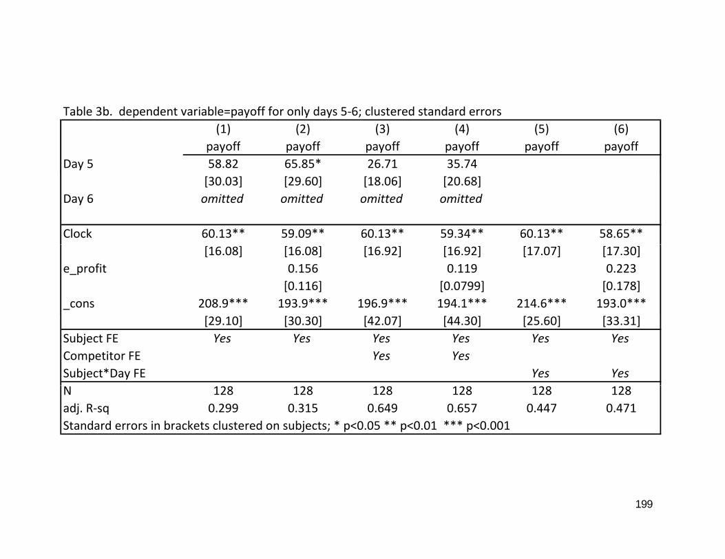
Table 3b. dependent variable=payoff for only days 5‐6; clustered standard errors(1) (2) (3) (4) (5) (6)
payoff payoff payoff payoff payoff payoffDay 5 58.82 65.85* 26.71 35.74
[30.03] [29.60] [18.06] [20.68]Day 6 omitted omitted omitted omitted
Clock 60.13** 59.09** 60.13** 59.34** 60.13** 58.65**[16.08] [16.08] [16.92] [16.92] [17.07] [17.30]
e_profit 0.156 0.119 0.223[0.116] [0.0799] [0.178]
_cons 208.9*** 193.9*** 196.9*** 194.1*** 214.6*** 193.0***[29.10] [30.30] [42.07] [44.30] [25.60] [33.31]
Subject FE Yes Yes Yes Yes Yes YesCompetitor FE Yes YesSubject*Day FE Yes YesN 128 128 128 128 128 128adj. R‐sq 0.299 0.315 0.649 0.657 0.447 0.471Standard errors in brackets clustered on subjects; * p<0.05 ** p<0.01 *** p<0.001
199
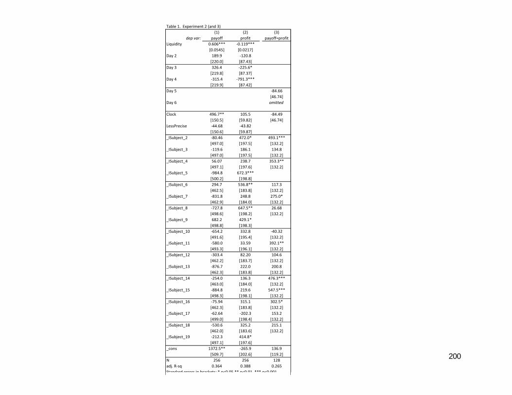
Table 1. Experiment 2 (and 3)(1) (2) (3)
dep var: payoff profit payoff=profitLiquidity 0.606*** ‐0.119***
[0.0545] [0.0217]Day 2 189.9 ‐120.8
[220.0] [87.43]Day 3 326.4 ‐225.6*
[219 8] [87 37][219.8] [87.37]Day 4 ‐315.4 ‐791.3***
[219.9] [87.42]Day 5 ‐84.66
[46.74]Day 6 omitted
Clock 496.7** 105.5 ‐84.49[150.5] [59.82] [46.74]
LessPrecise ‐44.68 ‐43.82[150.6] [59.87]
_ISubject_2 ‐80.46 472.0* 493.1***[497.0] [197.5] [132.2]
_ISubject_3 ‐119.6 186.1 134.8[497.0] [197.5] [132.2]
_ISubject_4 56.07 238.7 353.3**[497.1] [197.6] [132.2]
ISubject 5 984 8 672 3***_ISubject_5 ‐984.8 672.3***[500.2] [198.8]
_ISubject_6 294.7 536.8** 117.3[462.5] [183.8] [132.2]
_ISubject_7 ‐831.8 248.8 275.0*[462.9] [184.0] [132.2]
_ISubject_8 ‐727.8 647.5** 26.68[498.6] [198.2] [132.2]
_ISubject_9 682.2 429.1*[498.8] [198.3]
_ISubject_10 ‐654.2 332.8 ‐40.32[491.6] [195.4] [132.2]
_ISubject_11 ‐580.0 33.59 392.1**[493.3] [196.1] [132.2]
_ISubject_12 ‐303.4 82.20 104.6[462.2] [183.7] [132.2]
_ISubject_13 ‐876.7 222.0 200.8[462 3] [183 8] [132 2][462.3] [183.8] [132.2]
_ISubject_14 ‐254.0 136.3 476.3***[463.0] [184.0] [132.2]
_ISubject_15 ‐884.8 219.6 547.5***[498.3] [198.1] [132.2]
_ISubject_16 ‐75.94 315.1 302.5*[462.3] [183.8] [132.2]
_ISubject_17 ‐62.64 ‐202.3 153.2[499.0] [198.4] [132.2]
200
_ISubject_18 ‐530.6 325.2 215.1[462.0] [183.6] [132.2]
_ISubject_19 ‐212.3 414.8*[497.1] [197.6]
_cons 1372.5** ‐265.9 136.9[509.7] [202.6] [119.2]
N 256 256 128adj. R‐sq 0.364 0.388 0.265Standard errors in brackets; * p<0 05 ** p<0 01 *** p<0 001
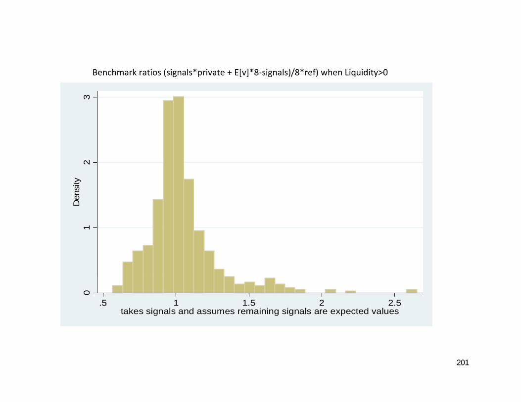
Benchmark ratios (signals*private + E[v]*8‐signals)/8*ref) when Liquidity>0Benchmark ratios (signals private + E[v] 8 signals)/8 ref) when Liquidity>0
32
Den
sity
10
.5 1 1.5 2 2.5takes signals and assumes remaining signals are expected values
201
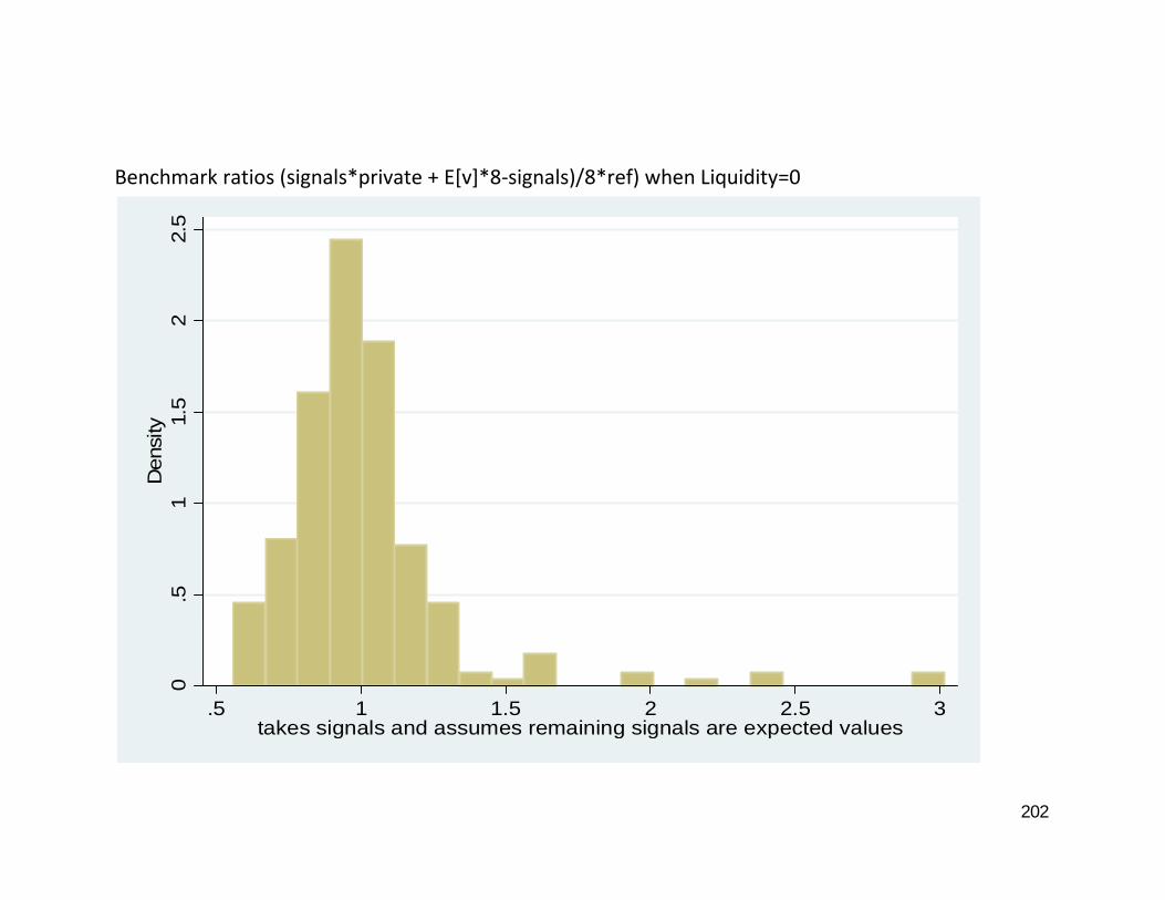
Benchmark ratios (signals*private + E[v]*8‐signals)/8*ref) when Liquidity=02.
52
11.
5D
ensi
ty.5
0
.5 1 1.5 2 2.5 3takes signals and assumes remaining signals are expected values
202
takes signals and assumes remaining signals are expected values
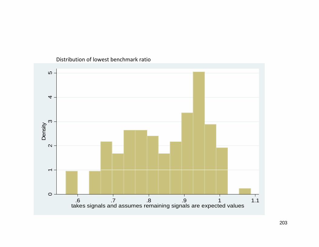
Distribution of lowest benchmark ratio
54
3D
ensi
ty1
2D
01
6 7 8 9 1 1 1
203
.6 .7 .8 .9 1 1.1takes signals and assumes remaining signals are expected values
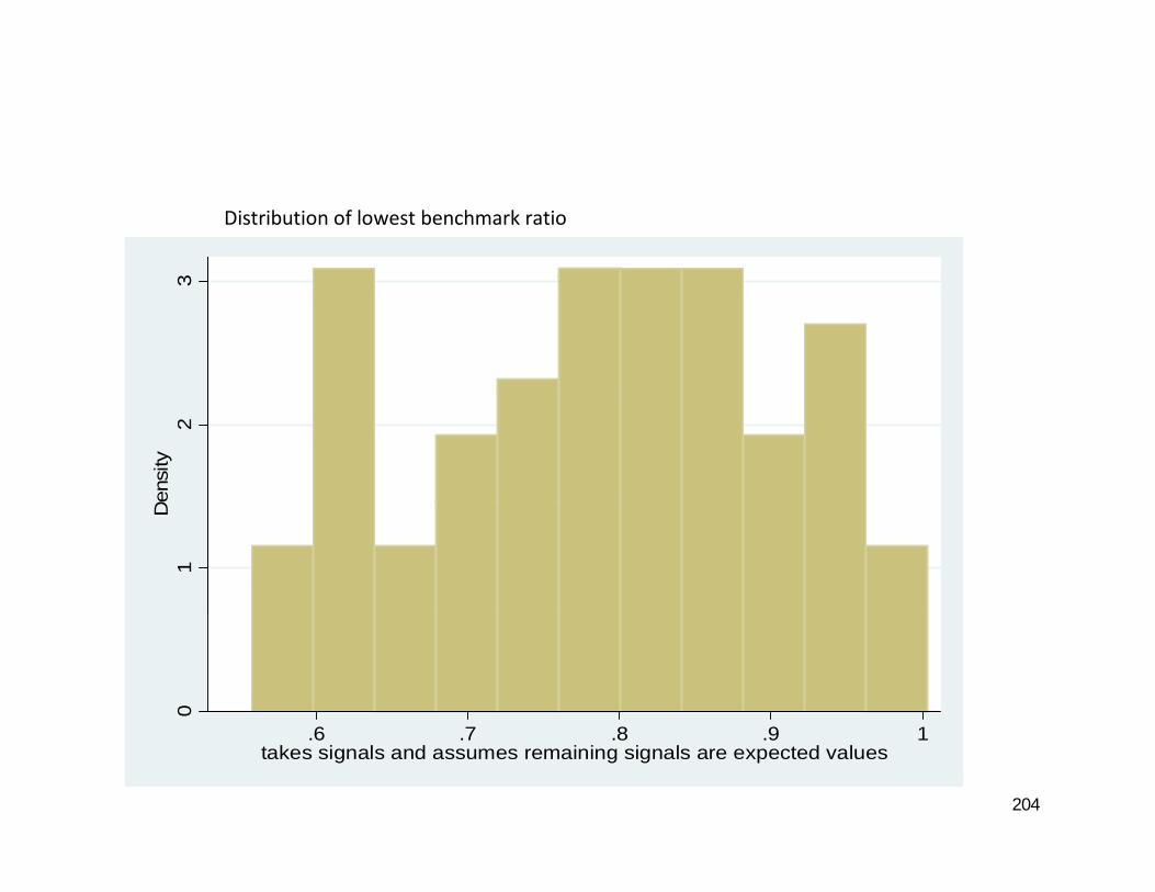
Distribution of lowest benchmark ratio
332
Den
sity
1D
0
6 7 8 9 1
204
.6 .7 .8 .9 1takes signals and assumes remaining signals are expected values
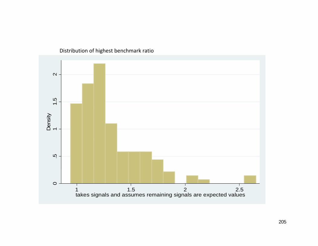
Distribution of highest benchmark ratio2
1.5
1Den
sity
.50
1 1.5 2 2.5takes signals and assumes remaining signals are expected values
205
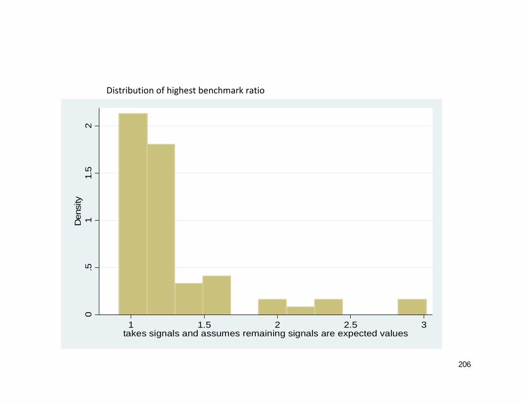
Distribution of highest benchmark ratio2
1.5
21
1D
ensi
ty.5
0
1 1.5 2 2.5 3
206
takes signals and assumes remaining signals are expected values
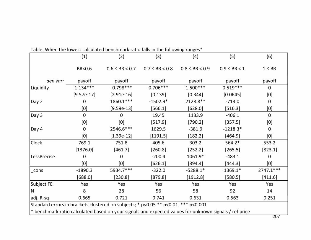
Table. When the lowest calculated benchmark ratio falls in the following ranges*(1) (2) (3) (4) (5) (6)
BR<0.6 0.6 ≤ BR < 0.7 0.7 ≤ BR < 0.8 0.8 ≤ BR < 0.9 0.9 ≤ BR < 1 1 ≤ BR
dep var: payoff payoff payoff payoff payoff payoffLiquidity 1.134*** ‐0.798*** 0.706*** 1.500*** 0.519*** 0
[9.57e‐17] [2.91e‐16] [0.139] [0.344] [0.0645] [0]Day 2 0 1860.1*** ‐1502.9* 2128.8** ‐713.0 0
[0] [9.59e‐13] [566.1] [628.0] [516.3] [0]Day 3 0 0 19.45 1133.9 ‐406.1 0
[0] [0] [517.9] [790.2] [357.5] [0]Day 4 0 2546.6*** 1629.5 ‐381.9 ‐1218.3* 0
[0] [1 39e 12] [1191 5] [182 2] [464 9] [0][0] [1.39e‐12] [1191.5] [182.2] [464.9] [0]Clock 769.1 751.8 405.6 303.2 564.2* 553.2
[1376.0] [461.7] [260.8] [252.2] [265.5] [823.1]LessPrecise 0 0 ‐200.4 1061.9* ‐483.1 0
[0] [0] [626.1] [394.4] [444.3] [0][ ] [ ] [ ] [ ] [ ] [ ]_cons ‐1890.3 5934.7*** ‐322.0 ‐5288.1* 1369.1* 2747.1***
[688.0] [230.8] [879.8] [1912.8] [580.5] [411.6]Subject FE Yes Yes Yes Yes Yes YesN 8 28 56 58 92 14
207
adj. R‐sq 0.665 0.721 0.741 0.631 0.563 0.251Standard errors in brackets clustered on subjects; * p<0.05 ** p<0.01 *** p<0.001* benchmark ratio calculated based on your signals and expected values for unknown signals / ref price
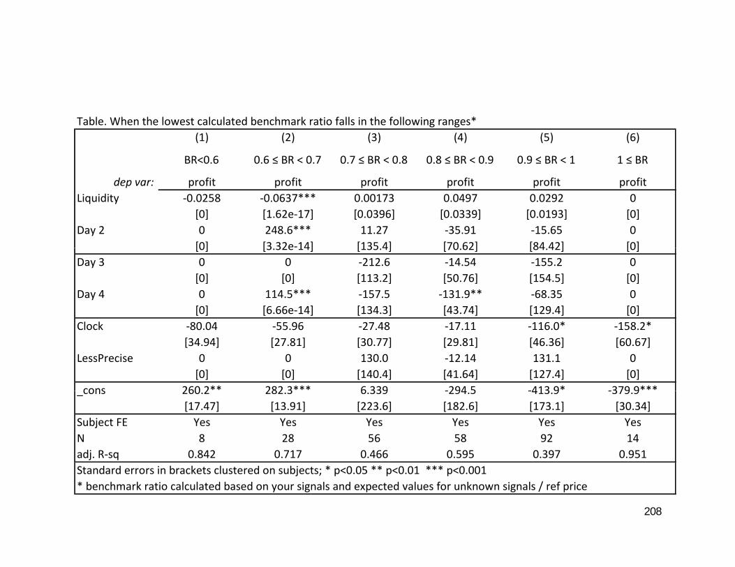
Table. When the lowest calculated benchmark ratio falls in the following ranges*(1) (2) (3) (4) (5) (6)
BR<0.6 0.6 ≤ BR < 0.7 0.7 ≤ BR < 0.8 0.8 ≤ BR < 0.9 0.9 ≤ BR < 1 1 ≤ BR
dep var: profit profit profit profit profit profitLiquidity ‐0.0258 ‐0.0637*** 0.00173 0.0497 0.0292 0
[0] [1.62e‐17] [0.0396] [0.0339] [0.0193] [0]Day 2 0 248.6*** 11.27 ‐35.91 ‐15.65 0
[0] [3 32e‐14] [135 4] [70 62] [84 42] [0][0] [3.32e 14] [135.4] [70.62] [84.42] [0]Day 3 0 0 ‐212.6 ‐14.54 ‐155.2 0
[0] [0] [113.2] [50.76] [154.5] [0]Day 4 0 114.5*** ‐157.5 ‐131.9** ‐68.35 0
[0] [6.66e‐14] [134.3] [43.74] [129.4] [0]Clock ‐80.04 ‐55.96 ‐27.48 ‐17.11 ‐116.0* ‐158.2*
[34.94] [27.81] [30.77] [29.81] [46.36] [60.67]LessPrecise 0 0 130.0 ‐12.14 131.1 0
[0] [0] [140.4] [41.64] [127.4] [0]cons 260 2** 282 3*** 6 339 ‐294 5 ‐413 9* ‐379 9***_cons 260.2 282.3 6.339 ‐294.5 ‐413.9 ‐379.9
[17.47] [13.91] [223.6] [182.6] [173.1] [30.34]Subject FE Yes Yes Yes Yes Yes YesN 8 28 56 58 92 14adj. R‐sq 0.842 0.717 0.466 0.595 0.397 0.951
208
Standard errors in brackets clustered on subjects; * p<0.05 ** p<0.01 *** p<0.001* benchmark ratio calculated based on your signals and expected values for unknown signals / ref price

Table. Relative importance of 4‐Signal Security with Liquidity(1) (2) (3) (4)
dep var: payoff payoff profit profitdep var: payoff payoff profit profitLiquidity 0.601*** 0.594*** ‐0.0555* ‐0.0579*
[0.0801] [0.0731] [0.0209] [0.0213]BenchRatio ‐560.8 ‐386.5 ‐43.91 20.19
[305.6] [272.1] [75.23] [67.38]4 Signals = HighSec ‐213.7 2620.5* ‐396.8*** 645.2
[178.1] [974.6] [63.97] [445.8]4SigHighSec*BenchRatio ‐2797.6** ‐1028.5*
[925.4] [461.0]Day 2 218 3 161 1 142 1 163 1Day 2 218.3 161.1 ‐142.1 ‐163.1
[406.0] [390.2] [77.46] [84.65]Day 3 357.1 323.1 ‐186.5* ‐199.0*
[275.0] [264.6] [76.33] [72.62]Day 4 ‐257.4 ‐262.0 ‐418.2** ‐419.9**y
[295.6] [308.3] [118.3] [114.4]Clock 496.7* 496.7* ‐96.34* ‐96.34*
[198.2] [198.6] [42.76] [42.84]LessPrecise ‐12.08 22.94 ‐38.49 ‐25.62
[147 2] [143 3] [40 71] [43 71][147.2] [143.3] [40.71] [43.71]_cons 769.4 628.7 419.4 367.7
[660.5] [658.1] [209.9] [202.3]N 256 256 256 256adj. R‐sq 0.417 0.432 0.427 0.451
209
adj. R sq 0.417 0.432 0.427 0.451Standard errors in brackets clustered on subjects; * p<0.05 ** p<0.01 *** p<0.001* benchmark ratio calculated based on your signals and expected values for unknown signals / ref price
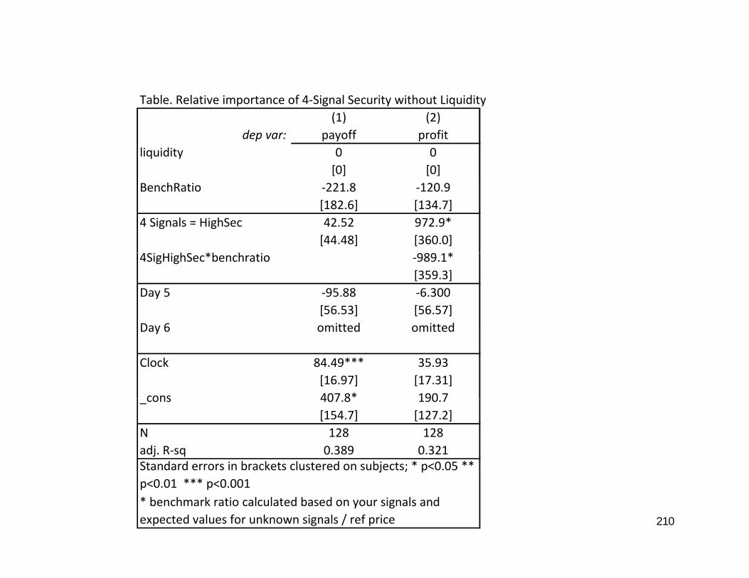
Table. Relative importance of 4‐Signal Security without Liquidity(1) (2)
dep var: payoff profitliquidity 0 0
[0] [0]BenchRatio ‐221.8 ‐120.9
[182.6] [134.7]4 Signals = HighSec 42.52 972.9*
[44.48] [360.0]h *b h *4SigHighSec*benchratio ‐989.1*
[359.3]Day 5 ‐95.88 ‐6.300
[56.53] [56.57]Day 6 omitted omittedDay 6 omitted omitted
Clock 84.49*** 35.93[16.97] [17.31]
cons 407 8* 190 7_cons 407.8 190.7[154.7] [127.2]
N 128 128adj. R‐sq 0.389 0.321Standard errors in brackets clustered on subjects; * p<0.05 **
210
* benchmark ratio calculated based on your signals and expected values for unknown signals / ref price
j ; pp<0.01 *** p<0.001