Embed Size (px)
Citation preview
HAL Id: hal-02429337https://hal.archives-ouvertes.fr/hal-02429337
Submitted on 6 Jan 2020
HAL is a multi-disciplinary open accessarchive for the deposit and dissemination of sci-entific research documents, whether they are pub-lished or not. The documents may come fromteaching and research institutions in France orabroad, or from public or private research centers.
L’archive ouverte pluridisciplinaire HAL, estdestinée au dépôt et à la diffusion de documentsscientifiques de niveau recherche, publiés ou non,émanant des établissements d’enseignement et derecherche français ou étrangers, des laboratoirespublics ou privés.
A comparative analysis of machine/deep learning modelsfor parking space availability prediction
Faraz Awan, Yasir Saleem, Roberto Minerva, Noel Crespi
To cite this version:Faraz Awan, Yasir Saleem, Roberto Minerva, Noel Crespi. A comparative analysis of ma-chine/deep learning models for parking space availability prediction. Sensors, MDPI, 2020, 20 (1),�10.3390/s20010322�. �hal-02429337�
sensors
Article
A Comparative Analysis of Machine/Deep LearningModels for Parking Space Availability Prediction
Faraz Malik Awan * , Yasir Saleem , Roberto Minerva and Noel Crespi
CNRS UMR5157, Telecom SudParis, Institut Polytechnique de Paris, 91000, Evry, France;[email protected] (Y.S.); [email protected] (R.M.);[email protected] (N.C.)* Correspondence: [email protected]; Tel.: +33-7533-8866-7
Received: 5 December 2019; Accepted: 1 January 2020; Published: 6 January 2020�����������������
Abstract: Machine/Deep Learning (ML/DL) techniques have been applied to large data sets in orderto extract relevant information and for making predictions. The performance and the outcomesof different ML/DL algorithms may vary depending upon the data sets being used, as well as onthe suitability of algorithms to the data and the application domain under consideration. Hence,determining which ML/DL algorithm is most suitable for a specific application domain and itsrelated data sets would be a key advantage. To respond to this need, a comparative analysis ofwell-known ML/DL techniques, including Multilayer Perceptron, K-Nearest Neighbors, DecisionTree, Random Forest, and Voting Classifier (or the Ensemble Learning Approach) for the prediction ofparking space availability has been conducted. This comparison utilized Santander’s parking data set,initiated while working on the H2020 WISE-IoT project. The data set was used in order to evaluatethe considered algorithms and to determine the one offering the best prediction. The results of thisanalysis show that, regardless of the data set size, the less complex algorithms like Decision Tree,Random Forest, and KNN outperform complex algorithms such as Multilayer Perceptron, in terms ofhigher prediction accuracy, while providing comparable information for the prediction of parkingspace availability. In addition, in this paper, we are providing Top-K parking space recommendationson the basis of distance between current position of vehicles and free parking spots.
Keywords: car parking; decision tree; deep learning; ensemble learning; IoT; K-nearest neighbors(KNN); machine learning; multilayer perceptron; parking sensors; random forest; sensors; smart city;voting classifier
1. Introduction
1.1. Background
One of the most challenging tasks associated with metropolitan cities like Paris or New York oreven smaller ones like Santander, Spain is to find an available parking space. According to an IBMsurvey [1], about 40% of the road traffic in cities is actually composed of vehicles whose drivers aresearching for parking spaces. This problem exacerbates issues such as fuel consumption, pollutionemission, road congestion, and wasted time, not to mention contributing to accidents due to the drivers’main focus on finding their space [2].
Much work has been done on parking space management, e.g., utilizing sensors (for determiningavailable parking spots) [3] and user feedback (i.e., people informing others of parking spaceavailability by means of applications) to identify available parking spaces [4]. Such systems arebased on transient data, without the possibility to actually reserve and allocate the parking spots,and so these techniques are only practical in very short timeframes and when the user is in close
Sensors 2020, 20, 322; doi:10.3390/s20010322 www.mdpi.com/journal/sensors
Sensors 2020, 20, 322 2 of 17
proximity to the parking areas. Even so, they do not offer any guarantee that a parking spot willbe available. However, to predict the availability of free parking spots at a particular time in thefuture, these systems coupled with Artificial Intelligence (AI)-based approaches can provide solutions.In order to succeed in the task of predicting parking space availability, data generated by the IoTsensors and the IoT devices, combined with ML/DL approaches, can be very useful. Given the varietyof ML/DL methods, one technical problem is to identify the most suitable ML/DL model for theproblem and the data set, as the performance of each ML/DL model varies from problem to problemand data set to data set. It is important to mention here some of the relevant works that have beendone on comparing AI/ML algorithms in several application domains. The use of ML/DL algorithmshas been compared for different application fields. For example, Hazar et al. [5] analyze automaticmodulation recognition over Rayleigh fading channels. They trained various ML/DL models for thistask, including Random Forest, KNN, Artificial Neural Networks (ANN), Support Vector Machines(SVM), Naïve Bayes, Gradient Boosted Regression Tree (GBRT), Hoeffding Tree, and Logistic regression,and found Naïve Bayes to be an optimal algorithm for this problem. While they ranked GBRT andLogistic Regression as the best algorithms in terms of recognition performance, these algorithmsrequired more processing time. Similarly, Naryanan et al. [6] applied Artificial Neural Network (ANN),KNN, and Support Vector Machine (SVM) approaches to a malware classification problem, and foundthat KNN outperformed SVM and ANN in terms of accuracy.
1.2. Contribution
In this paper, we analyze and evaluate various ML/DL models and determine the best predictivemodel among them for the parking space availability problem using the parking space data setof Santander, Spain. For comparison, we present different ML/DL-based solutions, includingKNN, Random Forest, Multilayer Perceptron (MLP), Decision Tree, and a combined model calledVoting Classifier (or Ensemble Learning). Although there are many ML/DL techniques availablein the literature, we chose these five ML/DL techniques because they are, firstly, well-known andwidely used in the community. Secondly, this is a preliminary work which we plan to extend forexperimentation and demonstration of the prediction of parking space availability by integratingit into Santander, Spain’s smart parking application for validation and to obtain user feedback.We performed this comparison using the well-known evaluation metrics Precision, Recall, F1-Score,and Accuracy. Our contributions are summarized below with respect to the main objective of predictingthe availability of parking spaces:• Identification of the best performing, among well-known and generally used ones, AI/ML
algorithm for the problem at hand;
– An analysis and evaluation of various ML/DL models (e.g.,KNN, Random Forest, MLP,Decision Tree) for the problem of predicting parking space availability;
– An analysis/assessment of the Ensemble Learning approach and its comparison with otherML/DL models; and
– Recommendation of the most appropriate ML/DL model to predict parking space availability.
• Recommending top-k parking spots with respect to distance between the current position ofvehicle and available parking spots;
• Application of the algorithms in order to demonstrate how satisfactory prediction of availabilityof parking spaces can be achieved using real data from Santander;
1.3. Impact of our Parking Prediction Model on Smart Cities
Smart Cities is a widely used term and is an umbrella that accommodates various aspects relatedto urban research. Mobility and Transportation are considered as the most important branches of theresearch related to smart cities. Smart transportation and mobility have the potential to make significantcontributions in smart cities by utilizing the Internet of Things (IoT) technologies. As described earlier,
Sensors 2020, 20, 322 3 of 17
drivers in search of parking space cause the traffic congestion, affecting many operations and domainsof smart cities such as route planning, traffic management, and parking spaces management. Here,the smart parking system makes an effort to reduce the traffic congestion on the roads [7] enrichedby our presented parking prediction ML/DL models that makes a significant impact on smart cities.Additionally, since our presented parking prediction models work on the data set of a smart city,Santander, therefore, it can have a direct impact on Santander smart city.
1.4. Organization
The organization of this paper is as follows. Section 2 presents the State of the Art. Section 3provides an overview of the five ML/DL techniques used for our analysis. The performance of theseML/DL techniques is presented in Section 4, and we provide our conclusions and recommendationsin Section 5.
2. Related Work
Many systems have been proposed to deal with the parking spot recommendation problem.The most common solution to this problem is a recommendation system based on real-time sensorscapable of detecting parking space availability [3]. For example, Yang et al. [8] evaluated a real-timeWireless Sensor Network (WSN) linked with a web server that collects the data for determiningthe available parking spots. These data are then passed on to users by means of a mobile phoneapplication. Similarly, Barone et al. [7] proposed an architecture, named Intelligent Parking Assistant(IPA). The proposed architecture does not provide parking spot availability prediction. In fact, it enablesusers to reserve a parking spot. In order to reserve a parking spot, the user is supposed to get registeredwith IPA; only the authorized user can use this architecture. Dong et al. [9] present a simulation-basedmethod, Parking Rank, to deal with the real-time detection of parking spots. Their system collectedthe public information of parking spots, e.g., price, total available space, rented space, etc. andsorted the parking spots by following the Page Rank algorithm. Since they are based on checkingreal-time data, these systems do not offer the possibility to predict the availability of a parking spacein an area and in a time frame (e.g., between 20 and 30 min from the current time) of interest of theuser. Therefore, other solutions have been suggested. A Neural Network based model (MLP) wasproposed by Vlahogianni et al. [10] to predict the occupancy rate of parking areas and parking spots.For example, in a specific parking area, there is a 75% probability that a parking space is going to beavailable in 5 min. Badii et al. [11] performed a comparative analysis of Bayesian Regularized NeuralNetwork, Support Vector Regression, Recurrent Neural Network, and Auto-regressive integratedmoving average methods for the prediction of parking spot availability within a specific garage withoutspecifying a particular parking spot. With ML/DL models, there are two different research directions:off-street parking spots and on-street parking spots [11]. Their approach is limited to parking spotsinside garages with gates (e.g., off-street parking spots). In addition, they included complex featureslike weather forecasts in their data set. Zheng et al. [12] performed a comparative analysis of RegressionTree, Neural Network, and Support Vector Regression (SVR) methods for the prediction of parkingoccupancy rates. Since they were dealing with the occupancy rate, while collecting the data theyfocused on information such as the number of occupied parking spaces. In terms of predictingthe parking occupancy rate, Zheng et al. found that the Regression Tree method outperforms theother two algorithms they evaluated. Camero et al. [13] presented a Recurrent Neural Network(RNN)-based approach to predict the number of free parking spaces. Their main aim was to improvethe performance of the RNN. To do so, they introduced a Genetic Algorithm (GA)-based techniqueand searched for the best configuration for RNN using the GA approach. They utilized the parkingdata of Birmingham, U.K., which contains the parking occupancy rate for each parking area given thetime and date. Yu et al. [14] selected the Auto Regressive Integrated Moving Average (ARIMA) modelto predict the number of berths available. ARIMA model is used for making time series forecast. Theirexperiment was based on a central mall’s underground parking and they collected one month data
Sensors 2020, 20, 322 4 of 17
(October 2010). As this is one month data, we believe it might not give clear insight as the parkingoccupancy pattern can vary in different months. We believe that different factors like public holidaysor other kinds of holidays can affect the performance, so one month data might not be enough tohave a clear view. Bibi et al. [15] performed car identification in a parking spot. They collectedthe video from the camera and divided the parking spots into blocks. Their main contribution is toidentify any parking spot it occupied or not using image processing. This processing is being donein real-time and does not provide any future prediction. However, their approach can be used fordata collection. Similarly, Tatulea et al. [16] detected the parking spaces and identified if the parkingspots are occupied or available using computer vision techniques and the camera as a sensor. In orderto do that, they performed different steps, including Frame Pre-processing, Adaptive BackgroundSubtraction, Metrics & Measurements, History Creation, Results Merging for Final Classification,and Parking Space Status. Again, this work is not about the future prediction of parking spots.
In contrast to the above-mentioned works, we deal with the prediction of on-street parking inSantander, a smart city of Spain and our prediction models are based on less complex data features.Moreover, we are targeting individual parking spot’s occupancy status and can make future predictionabout such spots with a validity period of 10 to 20 min. Our prediction has a 10 and 20 min validitybecause, according to our analysis, during peak hours, parking spots near places like city centersor shopping malls usually do not have the same status (free or occupied) for a longer time interval.Their status changes frequently with 10 to 20 min intervals.
3. Overview of ML/DL Techniques
Here, we provide an overview of the ML/DP techniques used to evaluate and analyze a data setin order to predict parking space availability. We compared the MLP, KNN, Decision Tree & RandomForest, and Ensemble Learning/Voting Classifier techniques.
3.1. Multilayer Perceptron (MLP) Neural Network
MLP is one of the most well-known types of neural networks. It consists of an input layer, one ormore hidden layer(s), and an output layer. Each hidden layer consists of multiple hidden units (alsocalled neurons or hidden nodes). The value of any hidden unit n in any hidden layer is calculatedusing Equation (1) [17]:
hn = a(N
∑K=1
iK ∗WK,n), (1)
where hn represents the output value of any hidden unit n in any hidden layer, and a representsthe activation function. The activation function is responsible for making the decision related to theactivation of a specific hidden unit. N in Equation (1) represents the total number of input nodes(in our case, there are five nodes in the input layer as well as in each of the three hidden layers), and iKrepresents the value of input node K being fed to hidden unit hn. This input node can be an inputlayer node or it can be a node in any previous hidden layer. WK,n represents the weight of unit hn.This weight is a measure of the connection strength between an input node and a hidden unit [18].
We used a Rectifier Linear Unit (ReLU) as the activation function for all the layers, so, at eachhidden unit, the activation function a in Equation (1), takes the input and returns the output valueas follows:
On = max(0, INPn), (2)
where On represents the output value of any hidden unit in any hidden layer, INPn = ∑NK=1 iK ∗WK,n
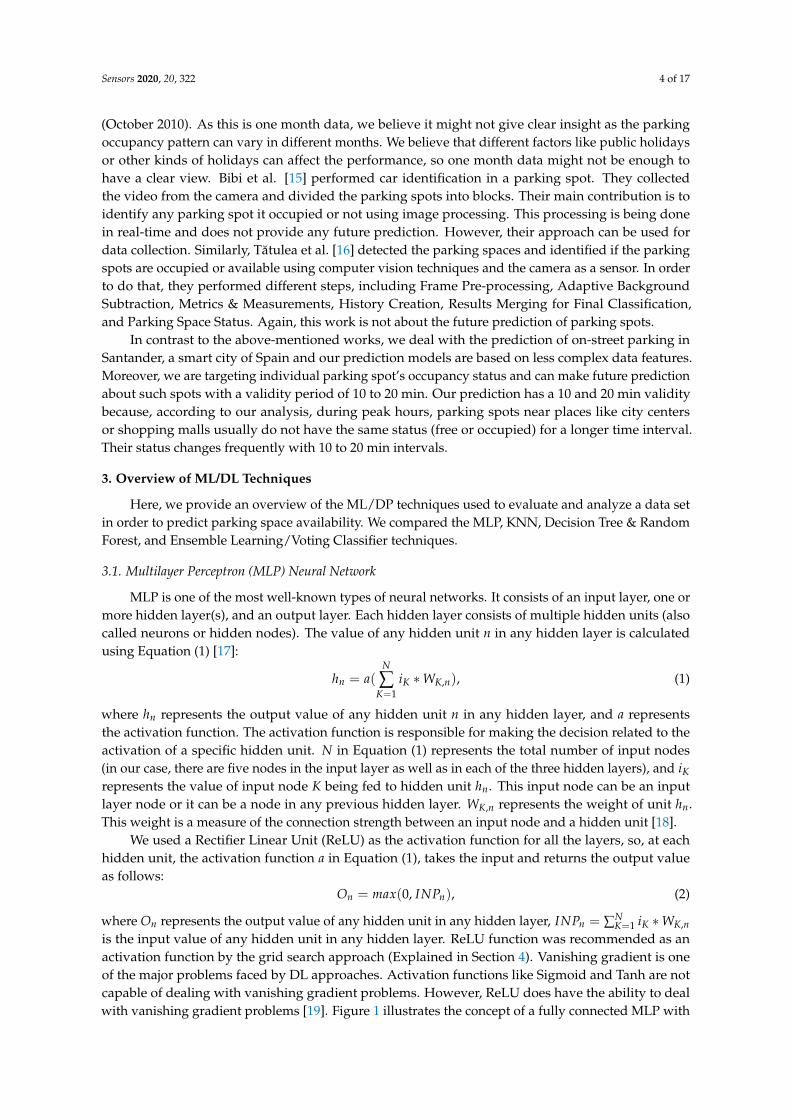
is the input value of any hidden unit in any hidden layer. ReLU function was recommended as anactivation function by the grid search approach (Explained in Section 4). Vanishing gradient is oneof the major problems faced by DL approaches. Activation functions like Sigmoid and Tanh are notcapable of dealing with vanishing gradient problems. However, ReLU does have the ability to dealwith vanishing gradient problems [19]. Figure 1 illustrates the concept of a fully connected MLP with
Sensors 2020, 20, 322 5 of 17
three hidden layers and with a number of hidden units equal to the number of features (x1, x2, . . . , xn)
in each sample in the data set. The complete details of these features are provided in Section 4.
Figure 1. MLP architecture.
3.2. K-Nearest Neighbors (KNN)
KNN is known as one of the simplest ML algorithms. It classifies samples on the basis of thedistances between them. In any classification data set, there are observations in the form of X and Y inthe training data, where Xi is the vector containing the feature values, and Yi is the class label againstXi. Let us suppose there is an observation Xk and we want to predict its class label Yk using KNN.Still using Equation (3), the KNN algorithm finds the K number of observations in X that are close(or similar) to the observation Xk:
DISTXk ,Xi = D(Xk, Xi)1≤i≤n. (3)
Using Equation (3), the distance between observation Xk and all the observations in X can becalculated. After calculating these distances, the top-K closest (similar) observations from the trainingdata are selected and then classed as the majority among the top-K closest observations is assigned tounlabeled sample Xk. There are several distance functions available, including Manhattan, Minkowski,and Euclidean [20]. Euclidean is the most popular; it calculates the distance between observationsusing Equation (4):
D(Xk, Xi) =
√√√√# f eatures
∑l=1
(Xl,k − Xl,i), (4)
where Xl,k represents the lth feature of sample Xk, and Xl,i represents the lth feature of observation Xi.
3.3. Decision Tree and Random Forest
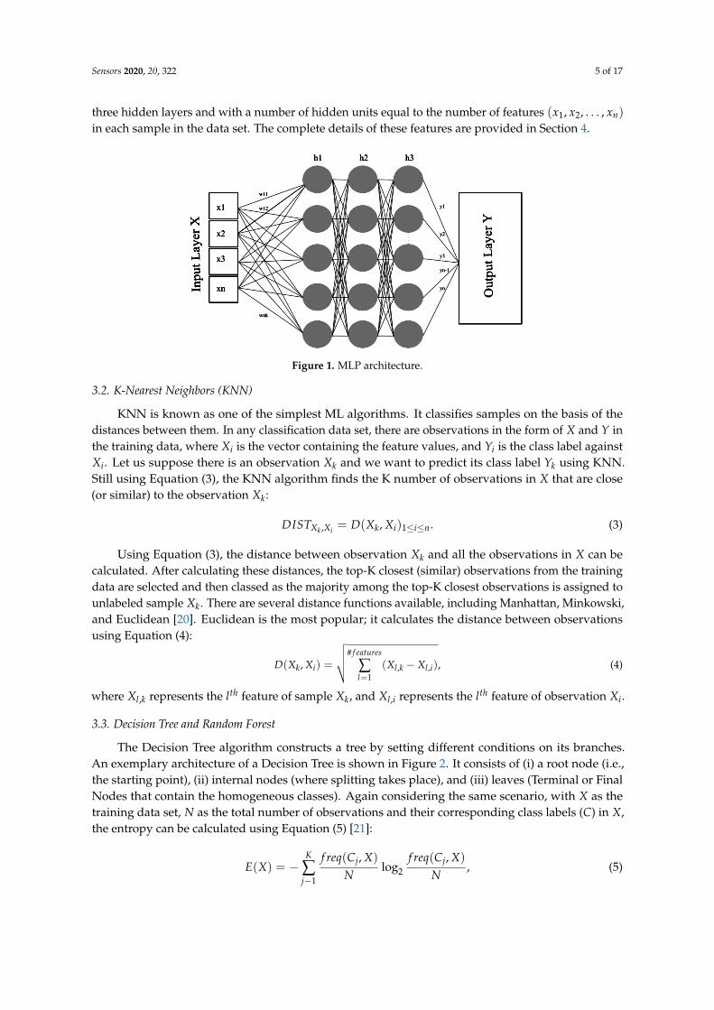
The Decision Tree algorithm constructs a tree by setting different conditions on its branches.An exemplary architecture of a Decision Tree is shown in Figure 2. It consists of (i) a root node (i.e.,the starting point), (ii) internal nodes (where splitting takes place), and (iii) leaves (Terminal or FinalNodes that contain the homogeneous classes). Again considering the same scenario, with X as thetraining data set, N as the total number of observations and their corresponding class labels (C) in X,the entropy can be calculated using Equation (5) [21]:
E(X) = −K
∑j−1
f req(Cj, X)
Nlog2
f req(Cj, X)
N, (5)
Sensors 2020, 20, 322 6 of 17
wheref req(Cj ,X)
N represents class Cj’s occurrence probability in X, and N represents the total number ofsamples in the training set. The information gain is then used to perform node split using equationsgiven in [21].
Figure 2. Decision tree architecture.
The Random Forest algorithm is similar to the Decision Tree algorithm. In fact, it consists ofmultiple independent Decision Trees. Each tree in a Random Forest sets conditional features differently.When a sample arrives at a root node, it is forwarded to all the sub-trees. Each sub-tree predicts theclass label for that particular sample. At the end, the class in the majority is assigned to that sample.
3.4. Ensemble Learning Approach (Voting Classifier)
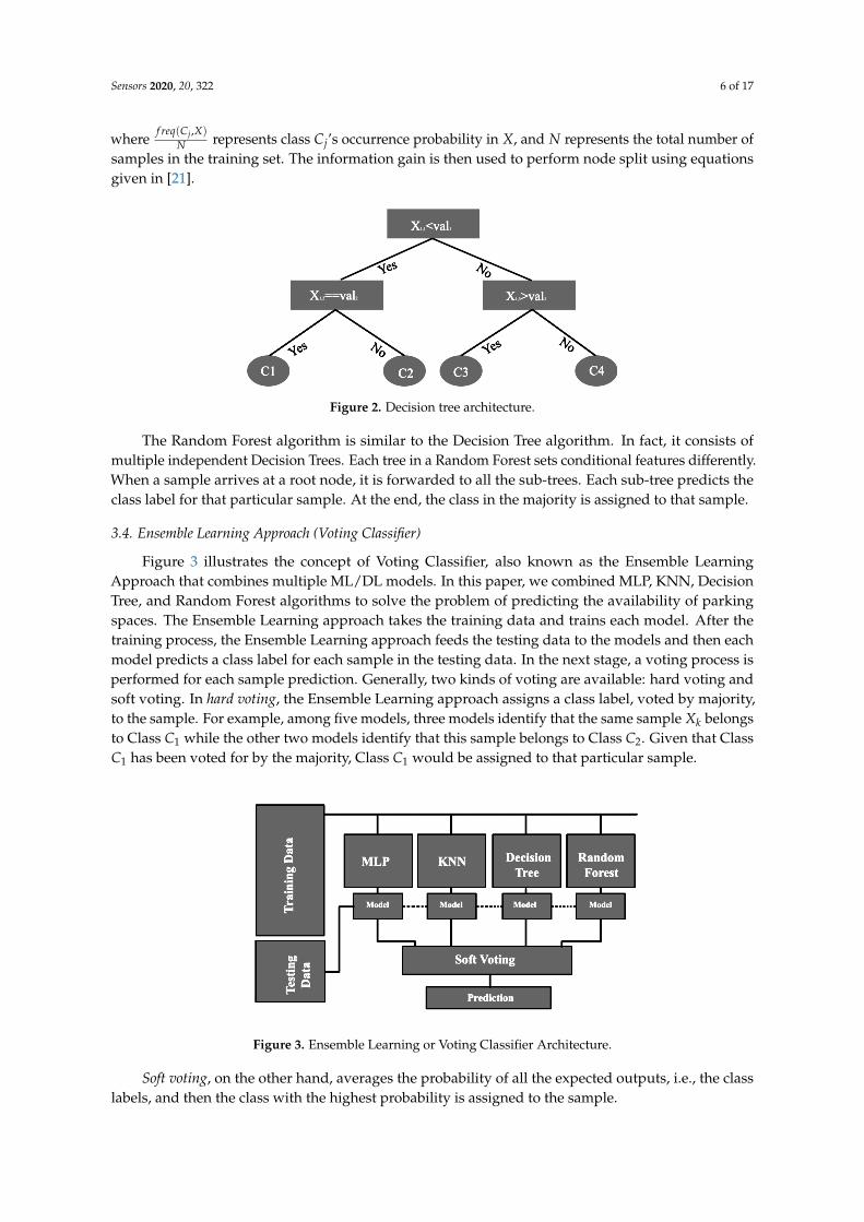
Figure 3 illustrates the concept of Voting Classifier, also known as the Ensemble LearningApproach that combines multiple ML/DL models. In this paper, we combined MLP, KNN, DecisionTree, and Random Forest algorithms to solve the problem of predicting the availability of parkingspaces. The Ensemble Learning approach takes the training data and trains each model. After thetraining process, the Ensemble Learning approach feeds the testing data to the models and then eachmodel predicts a class label for each sample in the testing data. In the next stage, a voting process isperformed for each sample prediction. Generally, two kinds of voting are available: hard voting andsoft voting. In hard voting, the Ensemble Learning approach assigns a class label, voted by majority,to the sample. For example, among five models, three models identify that the same sample Xk belongsto Class C1 while the other two models identify that this sample belongs to Class C2. Given that ClassC1 has been voted for by the majority, Class C1 would be assigned to that particular sample.
Figure 3. Ensemble Learning or Voting Classifier Architecture.
Soft voting, on the other hand, averages the probability of all the expected outputs, i.e., the classlabels, and then the class with the highest probability is assigned to the sample.
Sensors 2020, 20, 322 7 of 17
4. Results and Evaluation
During this work, the algorithms described in the previous section have been used, fine-tuned,analyzed and compared with respect to the specific goal of the recommendation system: i.e., to suggestdrivers the most probable and closest location to their final destination for a free parking space bylooking ahead in a specific time frame (e.g., 20 min times frame). Data were collected by sensorsdeployed in a real environment, i.e., the smart city Santander. In this section, we evaluate theperformance of five ML/DL models for the prediction of parking space availability and providea comparative analysis of the preliminary results, which we plan to extend by integrating them into asmart parking application for Santander, Spain for future experimentation.
4.1. Parking Space Data Set
The data set for the prediction was obtained by collecting the measurements of sensors deployedin Santander, a smart city in Spain. Almost 400 on-street parking sensors are deployed in the mainparking areas of the city center. These parking sensors [22] capture the status (i.e., occupied or free)of the parking spots. Collected over a 9-month period, this data set was constructed as part of theWISE-IoT [23], an H2020 EU-KR project. In WISE-IoT, the parking sensor data was stored in an NextGeneration Service Interface (NGSI) context broker [24]. We accessed real-time Santander data; in theWISE-IoT project, in order to make data more consistent, we created a script that retrieves and storesthe on-street parking sensor data every minute. The objective is twofold: to predict the parking spotavailability within a time interval (validity) of 10 to 20 min, and to evaluate the prediction accuracy.The collected data set has around 25 million records. We conducted our initial experiment using dataset having around 3 million records. Later on, in order to check the impact of larger data set on thealgorithms, the data set was extended to 25 million records. As scaling up the data set size did notaffect the standing (ranking) of ML/DL algorithms, we present the results for 25 million records in thePerformance Evaluation section. The collected data set has the following organization:
• Parking ID: Refers to the unique ID associated with each parking space.• Timestamp: The Timestamp of the parking space data collection.• Start Time/End Time: Start Time and End Time refer to the time interval during which a parking
space’s status remained the same, i.e., available or occupied.• Duration: Refers to the total duration in seconds during which a specific parking space remained
available or remained occupied.• Status: This feature represents the status of a parking space, e.g., available or occupied.
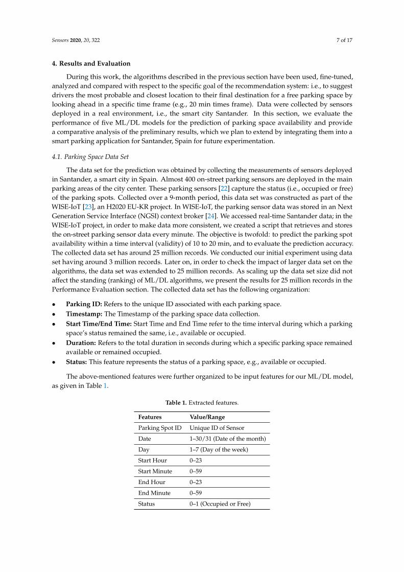
The above-mentioned features were further organized to be input features for our ML/DL model,as given in Table 1.
Table 1. Extracted features.
Features Value/Range
Parking Spot ID Unique ID of Sensor
Date 1–30/31 (Date of the month)
Day 1–7 (Day of the week)
Start Hour 0–23
Start Minute 0–59
End Hour 0–23
End Minute 0–59
Status 0–1 (Occupied or Free)
Sensors 2020, 20, 322 8 of 17
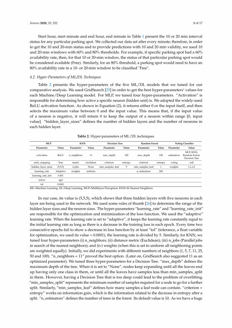
Start hour, start minute and end hour, end minute in Table 1 present the 10 or 20 min intervalstatus for any particular parking spot. We collected our data set after every minute; therefore, in orderto get the 10 and 20-min status and to provide predictions with 10 and 20 min validity, we used 10and 20-min windows with 60% and 80% thresholds. For example, if specific parking spot had a 60%availability rate, then, for that 10 or 20-min window, the status of that particular parking spot wouldbe considered available (Free). Similarly, for an 80% threshold, a parking spot would need to have an80% availability rate in a 10- or 20-min window to be classified "Free".
4.2. Hyper-Parameters of ML/DL Techniques
Table 2 presents the hyper-parameters of the five ML/DL models that we tuned for ourcomparative analysis. We used GridSearch [25] in order to get the best hyper-parameters’ values foreach Machine/Deep Learning model. For MLP, we tuned four hyper-parameters. “Activation” isresponsible for determining how active a specific neuron (hidden unit) is. We adopted the widely-usedReLU activation function. As shown in Equation (2), it returns either 0 or the input itself, and thenselects the maximum value between 0 and the input value. This means that, if the input valueof a neuron is negative, it will return 0 to keep the output of a neuron within range [0, inputvalue]. “hidden_layer_sizes” defines the number of hidden layers and the number of neurons ineach hidden layer.
Table 2. Hyper-parameters of ML/DL techniques.
MLP KNN Decision Tree Random Forest Voting Classifier
Parameter Value Parameter Value Parameter Value Parameter Value Parameter Value
activation ReLU n_neighbors 11 max_depth 100 max_depth 100 estimatorsMLP, KNN,
Random Forest,Decision Tree
early_stopping True metric euclidean criterion entropy criterion entropy voting soft
hidden_layer_sizes (5,5,5) n-jobs None min_samples_leaf 5 min_samples_leaf 1 weights 1,1,1,2
learning_rate Adaptive weights uniform n_estimators 200
learning_rate_init 0.001
solver sgd
tol 0.0001
ML=Machine Learning, DL=Deep Learning, MLP=Multilayer Perceptron, KNN=K-Nearest Neighbors
In our case, its value is (5,5,5), which shows that three hidden layers with five neurons in eachlayer are being used in the network. We used some rules of thumb [26] to determine the range of thehidden layer sizes and the neuron sizes. The hyper-parameters “learning_rate” and “learning_rate_init”are responsible for the optimization and minimization of the loss function. We used the “adaptive”learning rate. When the learning rate is set to “adaptive”, it keeps the learning rate constantly equal tothe initial learning rate as long as there is a decrease in the training loss in each epoch. Every time twoconsecutive epochs fail to show a decrease in loss function by at least “tol” (tolerance, a float variablefor optimization, we used its value = 0.0001), the learning rate is divided by 5. Similarly, for KNN, wetuned four hyper-parameters (i) n_neighbors; (ii) distance metric (Euclidean); (iii) n_jobs (Parallel jobsin search of the nearest neighbors); and (iv) weights (when this is set to uniform all neighboring pointsare weighted equally). Initially, we did experiments with different numbers of neighbors (1, 5, 7, 11, 25,50 and 100). “n_neighbors = 11” proved the best option. (Later on, GridSearch also suggested 11 as anoptimized parameter). We tuned three hyper-parameters for a Decision Tree. “max_depth” defines themaximum depth of the tree. When it is set to “None”, nodes keep expanding until all the leaves endup having only one class in them, or until all the leaves have samples less than min_samples_splitin them. However, having a Decision Tree that is too deep could lead to the problem of overfitting.“min_samples_split” represents the minimum number of samples required for a node to go for a furthersplit. Similarly, “min_samples_leaf” defines how many samples a leaf node can contain. “criterion =entropy” works on information gain, which is the information related to the decrease in entropy after asplit. “n_estimators” defines the number of trees in the forest. Its default value is 10. As we have a huge
Sensors 2020, 20, 322 9 of 17
data set (∼25 million records), we keep the number of estimators close to the usually-recommendedrange for a huge data set (i.e., 128 to 200). For an Ensemble Learning approach, the hyper-parameter“estimators” defines the ML/DL models to be used for prediction, while the hyper-parameter “weights”defines the priority given to each estimator. We assigned equal weights to all the estimators exceptDecision Tree. We gave Decision Tree a higher priority, as it performed relatively better than the restof the ML/DL models when it was used alone for parking space prediction. The hyper-parameter“voting” is described in Section 3.
4.3. Evaluation Metrics
The performance metrics we used for the evaluation and comparison of ML/DL models aregiven below. Moreover, to check the overfitting and stability of these models, we performed K-foldcross-validation. Each evaluation metric and K-fold cross-validation are explained below:
• Precision can be defined as the fraction of all the samples labelled as positive and that are actuallypositive [27]. It can be mathematically presented as follows:
Precision =TruePositive
TruePositive + FalsePositive. (6)
• Recall, in contrast, is defined as the fraction of all the positive samples; they are also labeled aspositive [27]. Mathematical presentation of recall is given below:
Recall =TruePositive
TruePositive + FalseNegative. (7)
• The F1-Score is defined as the harmonic mean of recall and precision [27], defined mathematically as:
F1− Score =2 ∗ (Recall ∗ Precision)
Recall + Precision. (8)
• Accuracy is the measure of the correctly predicted samples among all the samples, expressed in anequation as:
Accuracy =#CorrectPredictions
#TotalSamples. (9)
• K-fold cross-validation is a method for checking the overfitting and evaluating how consistent aspecific model is. In K-fold validation, a data set is divided into K equal sets. Among those K sets,each set is used once as testing data and the remaining sets are used as training data. In this paper,we used 5-fold cross-validation.
4.4. Performance Evaluation
This section provides an evaluation of the performance of the MLP, KNN, decision tree,random forest, and Ensemble Learning algorithms in terms of scores related to each cross-validation.A comparative analysis for 10-min and 20-min prediction was done, considering 60% and 80%thresholds for both predictions.
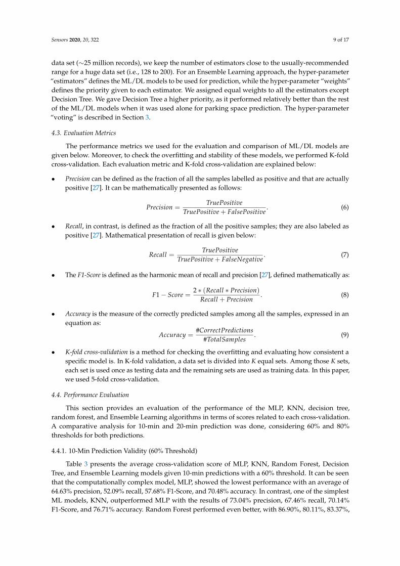
4.4.1. 10-Min Prediction Validity (60% Threshold)
Table 3 presents the average cross-validation score of MLP, KNN, Random Forest, DecisionTree, and Ensemble Learning models given 10-min predictions with a 60% threshold. It can be seenthat the computationally complex model, MLP, showed the lowest performance with an average of64.63% precision, 52.09% recall, 57.68% F1-Score, and 70.48% accuracy. In contrast, one of the simplestML models, KNN, outperformed MLP with the results of 73.04% precision, 67.46% recall, 70.14%F1-Score, and 76.71% accuracy. Random Forest performed even better, with 86.90%, 80.11%, 83.37%,
Sensors 2020, 20, 322 10 of 17
and 86.50% for average precision, recall, F1-Score, and accuracy, respectively. Decision Tree’s andEnsemble Learning’s performances were quite close to each other. Decision Tree showed 91.12%average precision while Ensemble learning had 92.79% average precision. The average recall scores forDecision Tree and Ensemble Learning were 90.28% and 89.24%, respectively. The average F1-Scorefor Decision Tree was 90.69% while Ensemble Learning showed 90.98%. The average accuracy forDecision Tree was 92.25%, while Ensemble Learning, despite combining all the models, could achieve92.54% accuracy, an improvement of only 0.29%.
Table 3. Average cross validation score of each model (10-min prediction validity with a 60% threshold).
Metrics MLP KNN RF DT EL
Precision 64.63 73.04 86.90 91.12 92.79
Recall 52.09 67.46 80.11 90.28 89.24
F1-Score 57.68 70.14 83.37 90.69 90.98
Accuracy 70.48 76.71 86.50 92.25 92.54
MLP=Multilayer Perceptron, KNN=K-Nearest Neighbors,
RF= Random Forest, DT=Decision Tree, EL=Ensemble Learning
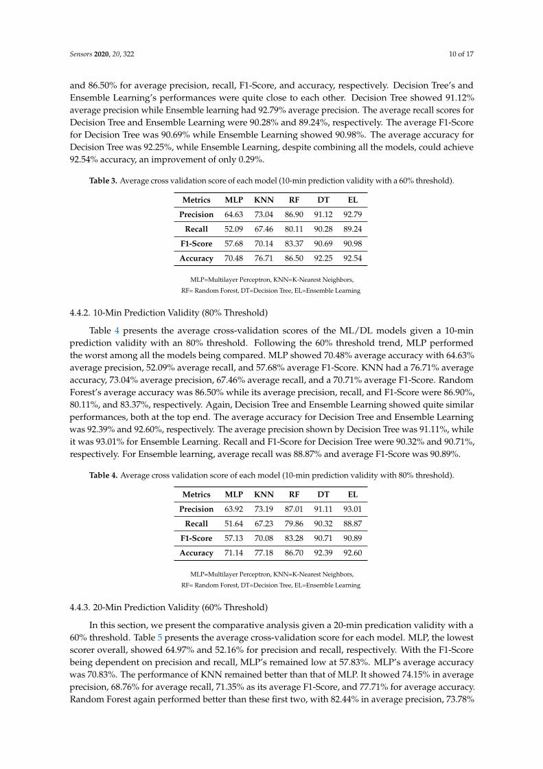
4.4.2. 10-Min Prediction Validity (80% Threshold)
Table 4 presents the average cross-validation scores of the ML/DL models given a 10-minprediction validity with an 80% threshold. Following the 60% threshold trend, MLP performedthe worst among all the models being compared. MLP showed 70.48% average accuracy with 64.63%average precision, 52.09% average recall, and 57.68% average F1-Score. KNN had a 76.71% averageaccuracy, 73.04% average precision, 67.46% average recall, and a 70.71% average F1-Score. RandomForest’s average accuracy was 86.50% while its average precision, recall, and F1-Score were 86.90%,80.11%, and 83.37%, respectively. Again, Decision Tree and Ensemble Learning showed quite similarperformances, both at the top end. The average accuracy for Decision Tree and Ensemble Learningwas 92.39% and 92.60%, respectively. The average precision shown by Decision Tree was 91.11%, whileit was 93.01% for Ensemble Learning. Recall and F1-Score for Decision Tree were 90.32% and 90.71%,respectively. For Ensemble learning, average recall was 88.87% and average F1-Score was 90.89%.
Table 4. Average cross validation score of each model (10-min prediction validity with 80% threshold).
Metrics MLP KNN RF DT EL
Precision 63.92 73.19 87.01 91.11 93.01
Recall 51.64 67.23 79.86 90.32 88.87
F1-Score 57.13 70.08 83.28 90.71 90.89
Accuracy 71.14 77.18 86.70 92.39 92.60
MLP=Multilayer Perceptron, KNN=K-Nearest Neighbors,
RF= Random Forest, DT=Decision Tree, EL=Ensemble Learning
4.4.3. 20-Min Prediction Validity (60% Threshold)
In this section, we present the comparative analysis given a 20-min predication validity with a60% threshold. Table 5 presents the average cross-validation score for each model. MLP, the lowestscorer overall, showed 64.97% and 52.16% for precision and recall, respectively. With the F1-Scorebeing dependent on precision and recall, MLP’s remained low at 57.83%. MLP’s average accuracywas 70.83%. The performance of KNN remained better than that of MLP. It showed 74.15% in averageprecision, 68.76% for average recall, 71.35% as its average F1-Score, and 77.71% for average accuracy.Random Forest again performed better than these first two, with 82.44% in average precision, 73.78%
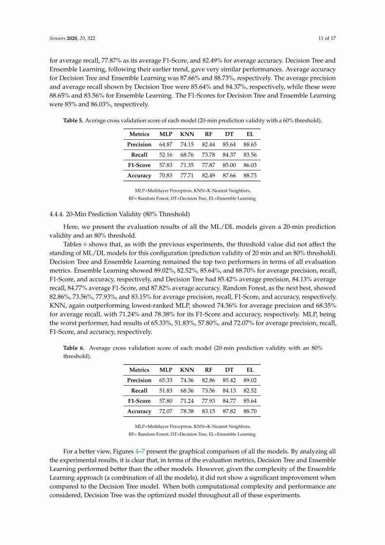
Sensors 2020, 20, 322 11 of 17
for average recall, 77.87% as its average F1-Score, and 82.49% for average accuracy. Decision Tree andEnsemble Learning, following their earlier trend, gave very similar performances. Average accuracyfor Decision Tree and Ensemble Learning was 87.66% and 88.73%, respectively. The average precisionand average recall shown by Decision Tree were 85.64% and 84.37%, respectively, while these were88.65% and 83.56% for Ensemble Learning. The F1-Scores for Decision Tree and Ensemble Learningwere 85% and 86.03%, respectively.
Table 5. Average cross validation score of each model (20-min prediction validity with a 60% threshold).
Metrics MLP KNN RF DT EL
Precision 64.87 74.15 82.44 85.64 88.65
Recall 52.16 68.76 73.78 84.37 83.56
F1-Score 57.83 71.35 77.87 85.00 86.03
Accuracy 70.83 77.71 82.49 87.66 88.73
MLP=Multilayer Perceptron, KNN=K-Nearest Neighbors,
RF= Random Forest, DT=Decision Tree, EL=Ensemble Learning
4.4.4. 20-Min Prediction Validity (80% Threshold)
Here, we present the evaluation results of all the ML/DL models given a 20-min predictionvalidity and an 80% threshold.
Tables 6 shows that, as with the previous experiments, the threshold value did not affect thestanding of ML/DL models for this configuration (prediction validity of 20 min and an 80% threshold).Decision Tree and Ensemble Learning remained the top two performers in terms of all evaluationmetrics. Ensemble Learning showed 89.02%, 82.52%, 85.64%, and 88.70% for average precision, recall,F1-Score, and accuracy, respectively, and Decision Tree had 85.42% average precision, 84.13% averagerecall, 84.77% average F1-Score, and 87.82% average accuracy. Random Forest, as the next best, showed82.86%, 73.56%, 77.93%, and 83.15% for average precision, recall, F1-Score, and accuracy, respectively.KNN, again outperforming lowest-ranked MLP, showed 74.36% for average precision and 68.35%for average recall, with 71.24% and 78.38% for its F1-Score and accuracy, respectively. MLP, beingthe worst performer, had results of 65.33%, 51.83%, 57.80%, and 72.07% for average precision, recall,F1-Score, and accuracy, respectively.
Table 6. Average cross validation score of each model (20-min prediction validity with an 80%threshold).
Metrics MLP KNN RF DT EL
Precision 65.33 74.36 82.86 85.42 89.02
Recall 51.83 68.36 73.56 84.13 82.52
F1-Score 57.80 71.24 77.93 84.77 85.64
Accuracy 72.07 78.38 83.15 87.82 88.70
MLP=Multilayer Perceptron, KNN=K-Nearest Neighbors,
RF= Random Forest, DT=Decision Tree, EL=Ensemble Learning
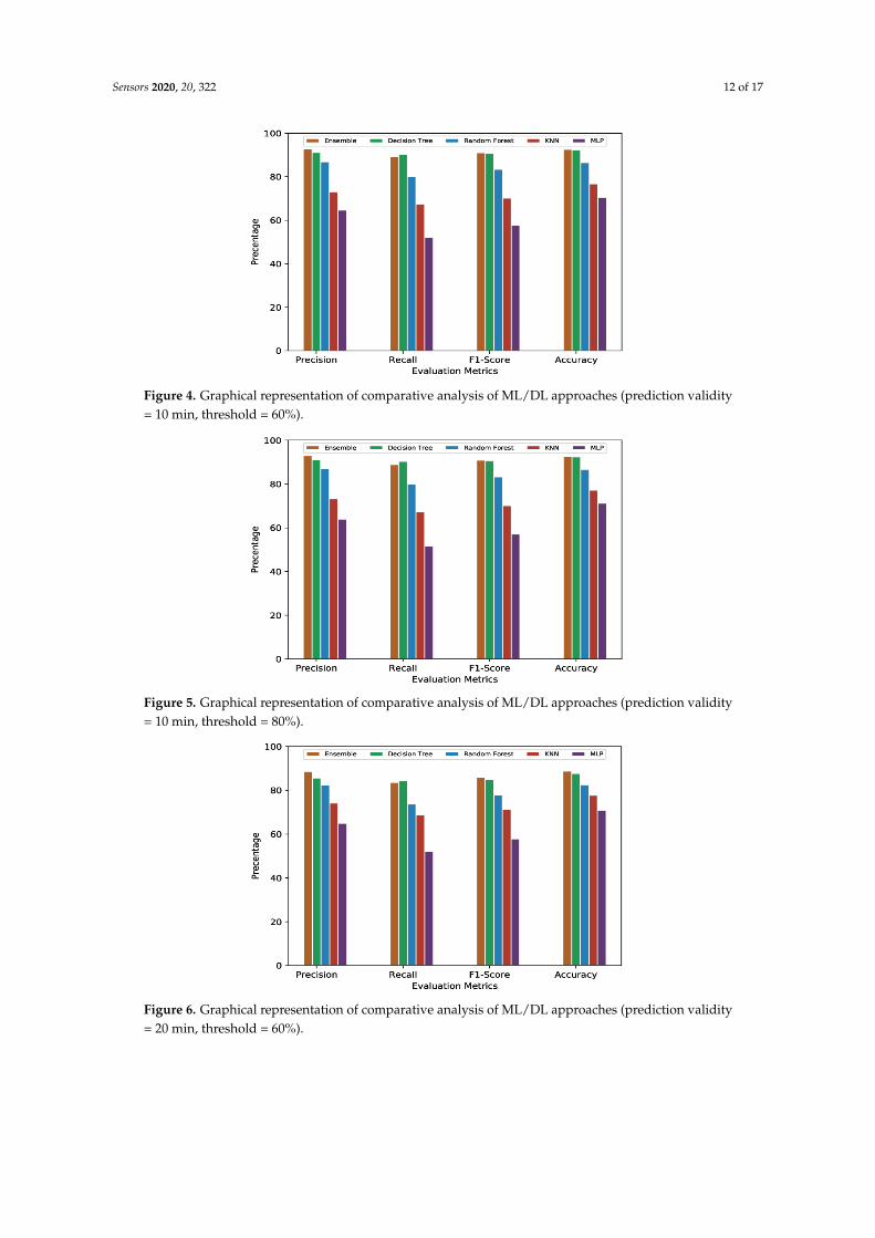
For a better view, Figures 4–7 present the graphical comparison of all the models. By analyzing allthe experimental results, it is clear that, in terms of the evaluation metrics, Decision Tree and EnsembleLearning performed better than the other models. However, given the complexity of the EnsembleLearning approach (a combination of all the models), it did not show a significant improvement whencompared to the Decision Tree model. When both computational complexity and performance areconsidered, Decision Tree was the optimized model throughout all of these experiments.
Sensors 2020, 20, 322 12 of 17
Figure 4. Graphical representation of comparative analysis of ML/DL approaches (prediction validity= 10 min, threshold = 60%).
Figure 5. Graphical representation of comparative analysis of ML/DL approaches (prediction validity= 10 min, threshold = 80%).
Figure 6. Graphical representation of comparative analysis of ML/DL approaches (prediction validity= 20 min, threshold = 60%).
Sensors 2020, 20, 322 13 of 17
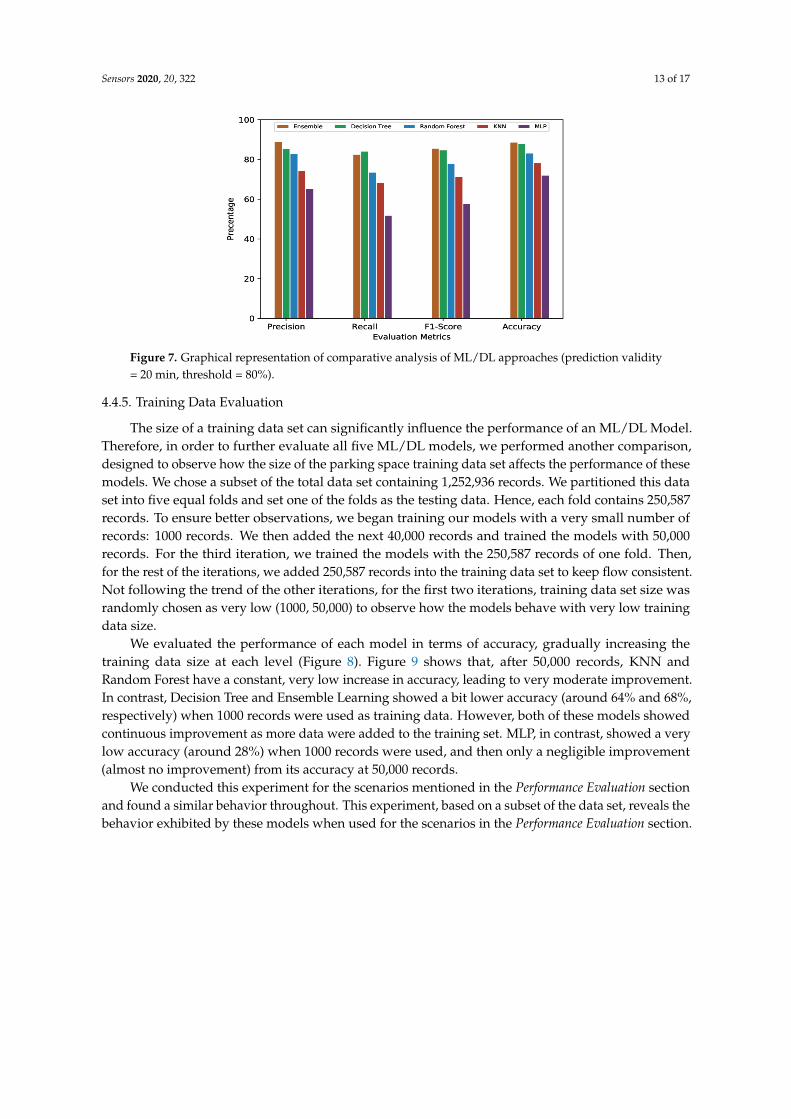
Figure 7. Graphical representation of comparative analysis of ML/DL approaches (prediction validity= 20 min, threshold = 80%).
4.4.5. Training Data Evaluation
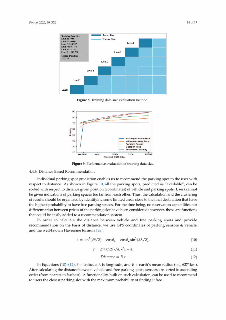
The size of a training data set can significantly influence the performance of an ML/DL Model.Therefore, in order to further evaluate all five ML/DL models, we performed another comparison,designed to observe how the size of the parking space training data set affects the performance of thesemodels. We chose a subset of the total data set containing 1,252,936 records. We partitioned this dataset into five equal folds and set one of the folds as the testing data. Hence, each fold contains 250,587records. To ensure better observations, we began training our models with a very small number ofrecords: 1000 records. We then added the next 40,000 records and trained the models with 50,000records. For the third iteration, we trained the models with the 250,587 records of one fold. Then,for the rest of the iterations, we added 250,587 records into the training data set to keep flow consistent.Not following the trend of the other iterations, for the first two iterations, training data set size wasrandomly chosen as very low (1000, 50,000) to observe how the models behave with very low trainingdata size.
We evaluated the performance of each model in terms of accuracy, gradually increasing thetraining data size at each level (Figure 8). Figure 9 shows that, after 50,000 records, KNN andRandom Forest have a constant, very low increase in accuracy, leading to very moderate improvement.In contrast, Decision Tree and Ensemble Learning showed a bit lower accuracy (around 64% and 68%,respectively) when 1000 records were used as training data. However, both of these models showedcontinuous improvement as more data were added to the training set. MLP, in contrast, showed a verylow accuracy (around 28%) when 1000 records were used, and then only a negligible improvement(almost no improvement) from its accuracy at 50,000 records.
We conducted this experiment for the scenarios mentioned in the Performance Evaluation sectionand found a similar behavior throughout. This experiment, based on a subset of the data set, reveals thebehavior exhibited by these models when used for the scenarios in the Performance Evaluation section.
Sensors 2020, 20, 322 14 of 17
Figure 8. Training data size evaluation method .
Figure 9. Performance evaluation of training data size.
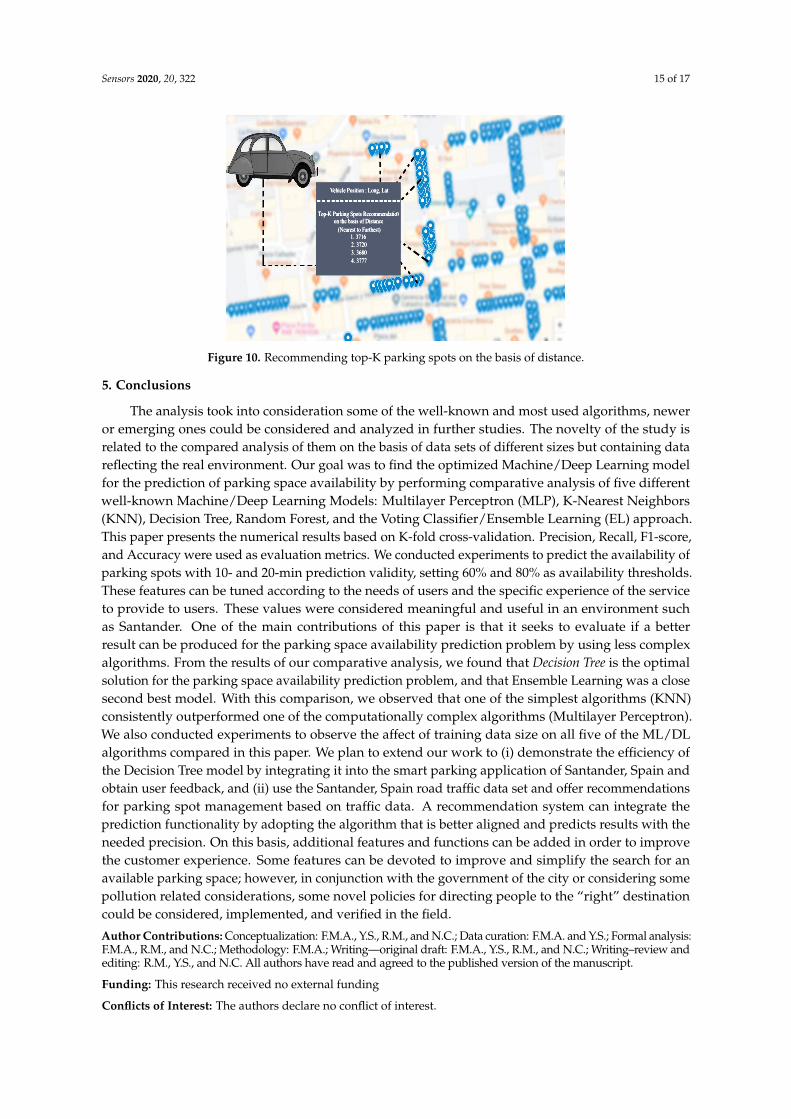
4.4.6. Distance Based Recommendation
Individual parking spot prediction enables us to recommend the parking spot to the user withrespect to distance. As shown in Figure 10, all the parking spots, predicted as “available”, can besorted with respect to distance given position (coordinates) of vehicle and parking spots. Users cannotbe given indications of parking spaces too far from each other. Thus, the calculation and the clusteringof results should be organized by identifying some limited areas close to the final destination that havethe highest probability to have free parking spaces. For the time being, no reservation capabilities nordifferentiation between prices of the parking slot have been considered; however, these are functionsthat could be easily added to a recommendation system.
In order to calculate the distance between vehicle and free parking spots and providerecommendation on the basis of distance, we use GPS coordinates of parking sensors & vehicle,and the well-known Haversine formula [28]:
a = sin2(δθ/2) + cos θ1 − cos θ2 sin2(δλ/2), (10)
c = 2a tan 2(√
a,√
1− a. (11)
Distance = R.c (12)
In Equations (10)–(12), θ is latitude, λ is longitude, and R is earth’s mean radius (i.e., 6371km).After calculating the distance between vehicle and free parking spots, sensors are sorted in ascendingorder (from nearest to farthest). A functionality, built on such calculation, can be used to recommendto users the closest parking slot with the maximum probability of finding it free.
Sensors 2020, 20, 322 15 of 17
Figure 10. Recommending top-K parking spots on the basis of distance.
5. Conclusions
The analysis took into consideration some of the well-known and most used algorithms, neweror emerging ones could be considered and analyzed in further studies. The novelty of the study isrelated to the compared analysis of them on the basis of data sets of different sizes but containing datareflecting the real environment. Our goal was to find the optimized Machine/Deep Learning modelfor the prediction of parking space availability by performing comparative analysis of five differentwell-known Machine/Deep Learning Models: Multilayer Perceptron (MLP), K-Nearest Neighbors(KNN), Decision Tree, Random Forest, and the Voting Classifier/Ensemble Learning (EL) approach.This paper presents the numerical results based on K-fold cross-validation. Precision, Recall, F1-score,and Accuracy were used as evaluation metrics. We conducted experiments to predict the availability ofparking spots with 10- and 20-min prediction validity, setting 60% and 80% as availability thresholds.These features can be tuned according to the needs of users and the specific experience of the serviceto provide to users. These values were considered meaningful and useful in an environment suchas Santander. One of the main contributions of this paper is that it seeks to evaluate if a betterresult can be produced for the parking space availability prediction problem by using less complexalgorithms. From the results of our comparative analysis, we found that Decision Tree is the optimalsolution for the parking space availability prediction problem, and that Ensemble Learning was a closesecond best model. With this comparison, we observed that one of the simplest algorithms (KNN)consistently outperformed one of the computationally complex algorithms (Multilayer Perceptron).We also conducted experiments to observe the affect of training data size on all five of the ML/DLalgorithms compared in this paper. We plan to extend our work to (i) demonstrate the efficiency ofthe Decision Tree model by integrating it into the smart parking application of Santander, Spain andobtain user feedback, and (ii) use the Santander, Spain road traffic data set and offer recommendationsfor parking spot management based on traffic data. A recommendation system can integrate theprediction functionality by adopting the algorithm that is better aligned and predicts results with theneeded precision. On this basis, additional features and functions can be added in order to improvethe customer experience. Some features can be devoted to improve and simplify the search for anavailable parking space; however, in conjunction with the government of the city or considering somepollution related considerations, some novel policies for directing people to the “right” destinationcould be considered, implemented, and verified in the field.
Author Contributions: Conceptualization: F.M.A., Y.S., R.M., and N.C.; Data curation: F.M.A. and Y.S.; Formal analysis:F.M.A., R.M., and N.C.; Methodology: F.M.A.; Writing—original draft: F.M.A., Y.S., R.M., and N.C.; Writing–review andediting: R.M., Y.S., and N.C. All authors have read and agreed to the published version of the manuscript.
Funding: This research received no external funding
Conflicts of Interest: The authors declare no conflict of interest.
Sensors 2020, 20, 322 16 of 17
References
1. IBM Survey. Available online: https://www-03.ibm.com/press/us/en/pressrelease/35515.wss (accessedon 20 August 2019).
2. Koster, A.; Oliveira, A.; Volpato, O.; Delvequio, V.; Koch, F. Recognition and recommendation of parkingplaces. In Proceedings of the Ibero-American Conference on Artificial Intelligence, Santiago de Chile, Chile,24–27 November 2014; pp. 675–685.
3. Park, W.; Kim, B.; Seo, D.; Kim, D.; Lee, K. Parking space detection using ultrasonic sensor inparking assistance system. In Proceedings of the 2008 IEEE Intelligent Vehicles Symposium, Eindhoven,The Netherlands, 4–6 June 2008; pp. 1039–1044, doi:10.1109/IVS.2008.4621296.
4. Rinne, M.; Törmä, S.; Kratinov, D. Mobile crowdsensing of parking space using geofencing and activityrecognition. In Proceedings of the 10th ITS European Congress, Helsinki, Finland, 16–19 June 2014; pp. 16–19.
5. Hazar, M.A.; Odabasioglu, N.; Ensari, T.; Kavurucu, Y.; Sayan, O.F. Performance analysis and improvementof machine learning algorithms for automatic modulation recognition over Rayleigh fading channels. NeuralComput. Appl. 2018, 29, 351–360, doi:10.1007/s00521-017-3040-6.
6. Narayanan, B.N.; Djaneye-Boundjou, O.; Kebede, T.M. Performance analysis of machine learning and patternrecognition algorithms for Malware classification. In Proceedings of the 2016 IEEE National Aerospace andElectronics Conference (NAECON) and Ohio Innovation Summit (OIS), Dayton, OH, USA, 25–29 July 2016;pp. 338–342, doi:10.1109/NAECON.2016.7856826.
7. Barone, R.E.; Giuffrè, T.; Siniscalchi, S.M.; Morgano, M.A.; Tesoriere, G. Architecture for parking managementin smart cities. IET Intell. Transp. Syst. 2013, 8, 445–452.
8. Yang, J.; Portilla, J.; Riesgo, T. Smart parking service based on Wireless Sensor Networks. In Proceedings ofthe 38th Annual Conference on IEEE Industrial Electronics Society, Montreal, QC, Canada, 25–28 October2012; pp. 6029–6034, doi:10.1109/IECON.2012.6389096.
9. Dong, S.; Chen, M.; Peng, L.; Li, H. Parking rank: A novel method of parking lotssorting and recommendation based on public information. In Proceedings of the IEEE InternationalConference on Industrial Technology (ICIT), Lyon, France, 20–22 February 2018; pp. 1381–1386,doi:10.1109/ICIT.2018.8352381.
10. Vlahogianni, E.; Kepaptsoglou, K.; Tsetsos, V.; Karlaftis, M. A Real-Time Parking Prediction System forSmart Cities. J. Intel. Transp. Syst. 2016, 20, 192–204, doi:10.1080/15472450.2015.1037955.
11. Badii, C.; Nesi, P.; Paoli, I. Predicting Available Parking Slots on Critical and Regular Services by Exploitinga Range of Open Data. IEEE Access 2018, 6, 44059–44071, doi:10.1109/ACCESS.2018.2864157.
12. Zheng, Y.; Rajasegarar, S.; Leckie, C. Parking availability prediction for sensor-enabled car parks in smartcities. In Proceedings of the IEEE Tenth International Conference on Intelligent Sensors, Sensor Networksand Information Processing (ISSNIP), Singapore, 7–9 April 2015; pp. 1–6.
13. Camero, A.; Toutouh, J.; Stolfi, D.H.; Alba, E. Evolutionary deep learning for car park occupancy predictionin smart cities. In Proceedings of the International Conference on Learning and Intelligent Optimization,Kalamata, Greece, 10–15 June 2018; pp. 386–401.
14. Yu, F.; Guo, J.; Zhu, X.; Shi, G. Real time prediction of unoccupied parking space using time series model.In Proceedings of the 2015 International Conference on Transportation Information and Safety (ICTIS),Wuhan, China, 25–28 June 2015; pp. 370–374.
15. Bibi, N.; Majid, M.N.; Dawood, H.; Guo, P. Automatic parking space detection system. In Proceedings ofthe 2017 2nd International Conference on Multimedia and Image Processing (ICMIP), Wuhan, China, 17–19March 2017; pp. 11–15.
16. Tatulea, P.; Calin, F.; Brad, R.; Brâncovean, L.; Greavu, M. An Image Feature-Based Method for Parking LotOccupancy. Future Internet 2019, 11, 169.
17. Huang, K.; Chen, K.; Huang, M.; Shen, L. Multilayer perceptron with particle swarm optimization for welllog data inversion. In Proceedings of the IEEE International Geoscience and Remote Sensing Symposium,Munich, Germany, 22–27 July 2012; pp. 6103–6106, doi:10.1109/IGARSS.2012.6352214.
18. Jain, A.K.; Mao, J.; Mohiuddin, K. Artificial neural networks: A tutorial. Computer 1996, 29, 31–44.19. Lau, M.M.; Lim, K.H. Investigation of activation functions in deep belief network. In Proceedings of the
2017 2nd International Conference on Control and Robotics Engineering (ICCRE), Bangkok, Thailand, 1–3April 2017; pp. 201–206.
Sensors 2020, 20, 322 17 of 17
20. Singh, A.; Yadav, A.; Rana, A. K-means with Three different Distance Metrics. Int. J. Comput. Appl. 2013, 67.21. Sharma, R.; Ghosh, A.; Joshi, P. Decision tree approach for classification of remotely sensed satellite data
using open source support. J. Earth Syst. Sci. 2013, 122, 1237–1247, doi:10.1007/s12040-013-0339-2.22. Santander Facility, Smart Santander. Available online: http://www.smartsantander.eu/index.php/testbeds/
item/132-santander-summary (accessed on 18 March 2019).23. Worldwide Interoperability for Semantics IoT (WISE-IoT), H2020 EU-KR Project . Available online: http:
//wise-iot.eu/en/home/ (accessed on 18 March 2019).24. Parking Sensors at Santander, Spain. Available online: https://mu.tlmat.unican.es:8443/v2/entities?limit=
1000&type=ParkingSpot (accessed on 15 June 2018).25. Scikit Learn. Available online: https://scikit-learn.org/stable/modules/generated/sklearn.model_selection.
GridSearchCV.html (accessed on 25 September 2019).26. Heaton, J. Artificial Intelligence for Humans, Volume 3: Deep Learning and Neural Networks; Artificial Intelligence
for Humans Series; CreateSpace Independent Publishing Platform: Scotts Valley, CA, USA, 2015.27. Lipton, Z.C.; Elkan, C.; Naryanaswamy, B. Optimal thresholding of classifiers to maximize F1 measure.
In Proceedings of the Joint European Conf. on Machine Learning and Knowledge Discovery in Databases,Nancy, France, 15–19 September 2014; pp. 225–239.
28. Yoga Swara, G.; others. Implementation Of Haversine Formula And Best First Search Method In SearchingOf Tsunami Evacuation Route. In Proceedings of the IOP Conference Series: Earth and EnvironmentalScience, Pekanbaru, Indonesia, 26–27 July 2017; Volume 97, p. 012004.
c© 2020 by the authors. Licensee MDPI, Basel, Switzerland. This article is an open accessarticle distributed under the terms and conditions of the Creative Commons Attribution(CC BY) license (http://creativecommons.org/licenses/by/4.0/).