A comparative study on ﬁnite elements for capturing strong ... J., A... · A comparative study on ﬁnite elements for capturing strong discontinuities: E-FEM vs X-FEM J. Oliver

www.elsevier.com/locate/cma

Comput. Methods Appl. Mech. Engrg. 195 (2006) 4732–4752

A comparative study on finite elements for capturingstrong discontinuities: E-FEM vs X-FEM

J. Oliver a,*, A.E. Huespe a, P.J. Sanchez b

a E.T.S. d’Enginyers de Camins, Canals i Ports, Technical University of Catalonia (UPC), Campus Nord UPC, Modul C-1,

c/Jordi Girona 1-3, 08034 Barcelona, Spainb CIMEC, CONICET, Guemes 3450, 3000 Santa Fe, Argentina

Received 8 March 2005; received in revised form 20 September 2005; accepted 20 September 2005

Abstract

A comparative study on finite elements for capturing strong discontinuities by means of elemental (E-FEM) or nodal enrichments (X-FEM) is presented. Based on the same constitutive model (continuum damage) and linear elements (triangles and tetrahedra) optimizedimplementations of both types of enrichments in the same non-linear code are tested for a representative set of 2D and 3D crack prop-agation examples. It is shown that both methods provide the same qualitative and quantitative results for enough refined meshes. For theperformed tests, E-FEM exhibited, in general, a higher accuracy, mostly for coarse meshes, whereas, convergence rate with mesh refine-ment, which is super-linear, showed slightly higher for X-FEM. As for the computational costs for single crack modelling X-FEMshowed, depending on the case, from 1.1 to about 2.5 times more expensive than E-FEM. For multiple cracks, the computational costof E-FEM keeps constant, whereas the cost associated to X-FEM increases linearly with the number of modelled cracks.� 2005 Elsevier B.V. All rights reserved.

Keywords: Finite elements with embedded discontinuities; E-FEM; X-FEM; Computational material failure; Strong discontinuities

1. Motivation

In recent years finite elements with discontinuities have gained increasing interest in modelling material failure, due totheir specific ability to provide, unlike standard finite elements, specific kinematics to capture strong discontinuities. Theyessentially consist of enriching the (continuous) displacement modes of the standard finite elements, with additional(discontinuous) displacements, devised for capturing the physical discontinuity i.e.: fractures, cracks, slip lines, etc. Thediscontinuity path is placed inside the elements irrespective of the size and specific orientation of them. Then, typical draw-backs of standard finite elements in modelling displacement discontinuities, like spurious mesh size and mesh bias depen-dences, can be effectively removed. In addition, unlike with standard elements, mesh refinement is not strictly necessary tocapture those discontinuities, and the simulation can be done with relatively coarse meshes. By using that technology, inconjunction with some additional refinements, realistic simulations of multiple strong discontinuities propagating in three-dimensional bodies can be achieved, with small computers, in reasonable computational times.

As for the enriching technique, two broad families can be distinguished in terms of the support of the enriching discon-tinuous displacement modes:

0045-7825/$ - see front matter � 2005 Elsevier B.V. All rights reserved.

doi:10.1016/j.cma.2005.09.020

* Corresponding author. Fax: +34 93 401 1048.E-mail address: [email protected] (J. Oliver).

mailto:[email protected]

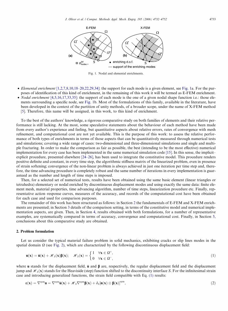
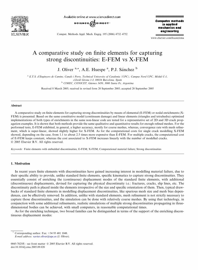
Fig. 1. Nodal and elemental enrichments.

J. Oliver et al. / Comput. Methods Appl. Mech. Engrg. 195 (2006) 4732–4752 4733

• Elemental enrichment [1,2,7,8,10,18–20,22,29,34]: the support for each mode is a given element, see Fig. 1a. For the pur-poses of identification of this kind of enrichment, in the remaining of this work it will be termed as E-FEM enrichment.

• Nodal enrichment [4,5,16,17,33,35]: the support of each mode is the one of a given nodal shape function i.e.: those ele-ments surrounding a specific node, see Fig. 1b. Most of the formulations of this family, available in the literature, havebeen developed in the context of the partition of unity methods, of a broader scope, under the name of X-FEM method[5]. Therefore, this name will be assigned, in this work, to this kind of enrichment.

To the best of the authors’ knowledge, a rigorous comparative study on both families of elements and their relative per-formance is still lacking. At the most, some speculative statements about the behaviour of each method have been madefrom every author’s experience and feeling, but quantitative aspects about relative errors, rates of convergence with meshrefinement, and computational cost are not yet available. This is the purpose of this work: to assess the relative perfor-mance of both types of enrichments in terms of those aspects that can be quantitatively measured through numerical testsand simulations; covering a wide range of cases: two-dimensional and three-dimensional simulations and single and multi-ple fracturing. In order to make the comparison as fair as possible, the best (intending to be the most effective) numericalimplementation for every case has been implemented in the same numerical simulation code [15]. In this sense, the implicit–explicit procedure, presented elsewhere [24–26], has been used to integrate the constitutive model. This procedure renderspositive definite and constant, in every time step, the algorithmic stiffness matrix of the linearized problem, even in presenceof strain softening; convergence of the non-linear problem is always achieved in just one iteration per time step and, there-fore, the time advancing procedure is completely robust and the same number of iterations in every implementation is guar-anteed as the number and length of time steps is imposed.

Then, for a selected set of numerical tests, results have been obtained using the same basic element (linear triangles ortetrahedra) elementary or nodal enriched by discontinuous displacement modes and using exactly the same data: finite ele-ment mesh, material properties, time advancing algorithm, number of time steps, linearization procedure etc. Finally, rep-resentative action–response curves, measures of the accuracy, and records of the computational cost have been obtainedfor each case and used for comparison purposes.

The remainder of this work has been structured as follows: in Section 2 the fundamentals of E-FEM and X-FEM enrich-ments are presented; in Section 3 details of the comparison setting, in terms of the constitutive model and numerical imple-mentation aspects, are given. Then, in Section 4, results obtained with both formulations, for a number of representativeexamples, are systematically compared in terms of accuracy, convergence and computational cost. Finally, in Section 5,conclusions about this comparative study are obtained.

2. Problem formulation

Let us consider the typical material failure problem in solid mechanics, exhibiting cracks or slip lines modes in thespatial domain X (see Fig. 2), which are characterized by the following discontinuous displacement field:

uðxÞ ¼ �uðxÞ þHSðxÞbðxÞ; HSðxÞ ¼1 8x 2 Xþ;

0 8x 2 X�;

�ð1Þ

where u stands for the displacement field, �u and b are, respectively, the regular displacement field and the displacementjump and HSðxÞ stands for the Heaviside (step) function shifted to the discontinuity interface S. For the infinitesimal straincase and introducing generalized functions, the strain field compatible with Eq. (1) results:

eðxÞ ¼ rsymu ¼ rsym�uðxÞ þHSrsymbðxÞ þ dS ½nðxÞ � bðxÞ�sym; ð2Þ

Fig. 2. Strong discontinuity kinematics.

4734 J. Oliver et al. / Comput. Methods Appl. Mech. Engrg. 195 (2006) 4732–4752

where n is normal to S and dS stands for the Dirac’s delta-function shifted to S. For the spatially discretized body, Xh, thevariational governing equation, in the standard form and in absence of body forces, reads:Z

Xhrsym duh � rdX ¼

ZCh

r

duh ��tdCr 8duh 2Vh0; ð3Þ

where Chr � oXh is the boundary with prescribed tractions, �t, and Vh

0 is the space of admissible displacements, which shouldbe appropriately defined. Both the displacement field (1) and the space Vh

0 are represented in different ways by the elemen-tal and nodal embedded strong discontinuity enrichments.

2.1. X-FEM enrichment

The space of interpolation functions is defined by

VhX-FEM ¼ uhðxÞjuhðxÞ ¼

Xnnode

i¼1

ðN iðxÞdi þHSN iðxÞbiÞ( )

; ð4Þ

Ni standing for the standard interpolation finite element shape functions, di are the nodal regular displacement vector, bi isthe nodal displacement jump vector and nnode is the number of nodes of the finite element mesh. The corresponding (infin-itesimal) strain field results:

ehðxÞ ¼ rsymuh ¼Xnnode

i¼1

½ðrN i � diÞsym þHSðrN i � biÞsym þ dSðn� NibiÞ

sym�. ð5Þ

Then the variations, with respect to parameters (di,bi) in Eq. (4) lead to the discrete equilibrium equations:

ddi �Z

XhrNi � rdX�

ZCh

r

Ni ��tdC

!¼ 0 8ddi; i ¼ 1; nnode;

dbi �Z

XhHSrN i � rdXþ

ZS

N i � ðrS � nÞdS� �

¼ 0 8dbi; i ¼ 1; nnode.

ð6Þ

The term rS � n ¼ tS , in Eq. (6b), can be interpreted as an interface cohesive traction.

2.2. E-FEM enrichment

In this approach, the discontinuous displacement is interpolated by using the following functional space:

VhE-FEM ¼ uhðxÞjuhðxÞ ¼

Xnnode

i¼1

ðNiðxÞdiÞ þXnelem

e¼1

MðeÞS be

( );

MðeÞS ¼HS � uðeÞ; uðeÞ ¼

XnðeÞnodeþ

i¼1

N ðeÞi ;

ð7Þ


where, nelem is the number of elements and nðeÞnodeþ refers to those nodes of element e placed in X+ (see Fig. 1). In Eq. (7) be

are degrees of freedom describing the elemental displacement jumps and MðeÞS is the so-called elemental unit jump function

whose support is the elemental domain X(e) [28]. The corresponding strain field reads:

ehðxÞ ¼ rsymuh ¼Xnnode

i¼1

ðrNi � diÞsym �Xnelem

e¼1

ð½ðruðeÞ � beÞsym � dSðn� beÞ

sym�Þ; ð8Þ

and variations, in Eq. (8), with respect to parameters (di,be) lead to the discrete variational equations defining a kinemat-ically consistent E-FEM implementation [10,13]:

ddi �Z

XhrNi � rdX�

ZCh

r

Ni ��tdC

!¼ 0 8ddi; i ¼ 1; nnode;

dbe �Z

XðeÞruðeÞ � rdXþ

ZSðeÞðrS � nÞdS

� �¼ 0 8dbe; e ¼ 1; nelem.

ð9Þ

3. Comparison setting

In order to make a rigorous comparison, a common comparison setting for both methods has to be defined in terms ofthe constitutive model, the numerical algorithms and the finite element implementation. This is described in next sections.

3.1. Constitutive model: degenerated traction-separation law

For the sake of simplicity, an isotropic continuum damage model, equipped with strain softening, has been chosen tomodel the mechanical behaviour of the material. The essentials of the model are the following:

uðe; rÞ ¼ 1

2

qðrÞrðe : C : eÞ ¼ 1

2

qðrÞrð�k tr2ðeÞ þ 2le : eÞ;

r ¼ ouðe; rÞoe

¼ qr|{z}

1�d

C : e ¼ ð1� dÞ C : e|ffl{zffl}�rðeÞ

ðeffective stressÞ

¼ ð1� dÞ�r

_r ¼ c; rðtÞjt¼t0� r0 ¼

ruffiffiffiffiEp ;

_q ¼ HðqÞ_r; qðtÞjt¼t0� q0 ¼ r0;

c P 0; Frðr; qÞ 6 0; cFr ¼ 0;

Frðr; qÞ ¼ sr � q; sr ¼ffiffiffiffiffiffiffiffiffiffiffiffiffiffiffiffiffiffiffiffiffiffiffiffirþ : C�1 : r

p|fflfflfflfflfflfflfflfflfflffl{zfflfflfflfflfflfflfflfflfflffl}equivalent stress

¼ qr

ffiffiffiffiffiffiffiffiffiffiffiffiffiffiffiffiffiffiffiffiffiffiffiffiffiffiffiffiffiffiffiffiffiffiffiffi�rþðeÞ : C�1 : �rðeÞ

q|fflfflfflfflfflfflfflfflfflfflfflfflfflfflfflffl{zfflfflfflfflfflfflfflfflfflfflfflfflfflfflfflffl}

equivalent strain se

;

ð10Þ

where u(e, r) is the free energy, depending on the strain tensor e, and the internal variable r, C ¼ �kð1� 1Þ þ 2lI is the elas-tic constitutive tensor, where �k and l are the Lame’s parameters and 1 and I are the identity tensors of second and fourthorder, respectively. In Eq. (10) d = 1 � q(r)/r is the continuum damage variable, r stands for the stress tensor and �r ¼ C : eis the effective stress tensor. Its positive counterpart is then defined as

�rþ ¼Xi¼3

i¼1

h�riipi � pi; ð11Þ

where h�rii stands for the positive part (Mac Auley bracket) of the ith principal effective stress �ri ðh�rii ¼ �ri for �ri > 0 andh�rii ¼ 0 for �ri < 0Þ and pi stands for the ith stress eigenvector. The initial elastic domain in the damage model is defined as

E0r :¼ fr;

ffiffiffiffiffiffiffiffiffiffiffiffiffiffiffiffiffiffiffiffiffiffiffiffirþ � Ce�1 � r

p< r0g and, therefore, it is unbounded for compressive stress states (r+ = 0) so that damage be-

comes only associated to tensile stress states as it is usual for modelling tensile failure in quasi-brittle materials. Materialsoftening is defined by the evolution of the internal variable q(r) in terms of the continuum softening modulus H(q) 6 0.Finally, ru and E are, respectively, the tensile strength and the Young’s modulus. One of the advantages of the previ-ous model, infrequent in non-linear constitutive models, is that the internal variable r can be integrated in closed form as

rðtÞ ¼ maxs2½0;t�

seðeðsÞ; r0Þ ð12Þ

and, from this, the complete constitutive model can be analytically integrated from Eq. (10).


In the context of the continuum strong discontinuity approach (CSDA) the preceding constitutive model should beadapted to return bounded stresses when the singular (unbounded) strain field (2) is introduced into the standard contin-uum context. This regularization is achieved by substituting the Dirac’s delta function dS by a regularized sequence,dS � lS=k ðk ! 0Þ, where lSðxÞ is a collocation function on the discontinuity interface SðlSðxÞ ¼ 1 8x 2 S andlSðxÞ ¼ 0 otherwise). In addition, the continuum softening modulus, H, in Eq. (10), is reinterpreted, in the distributionalsense [32] and, then, regularized as

HðqÞ ¼ kHðqÞ ð13Þin terms of a discrete softening modulus H , considered a material property available from the mechanical and fracturingproperties of the material (peak stress ru, Young modulus E, and fracture energy Gf; see [21,27] for additional details).

In this context it can be shown [21] that the following traction separation law, relating the traction, tS ¼ rS � n, and thedisplacement jump, b, is automatically fulfilled at the discontinuity interface S after activation of the strong discontinuitykinematics (2):

uSðb; aÞ ¼1

2

qðaÞa½b : Qe : b� ¼ 1

2

qðaÞa½ð�kþ lÞðb � nÞ2 þ lb � b�;

Qe ¼ n � C � n ¼ ð�kþ lÞn� nþ l1;

tS ¼ouSðb; aÞ

ob¼ q

a|{z}1�x

Qe � b ¼ ð1� xÞQe � b;

_a ¼ c; aðtÞjt¼tloc¼ 0;

_q ¼ HðqÞa; qðtÞjt¼tloc� qloc;

c P 0; Ftðt; qÞ 6 0; cFt ¼ 0;

Ftðt; qÞ ¼ st � q; st ¼ffiffiffiffiffiffiffiffiffiffiffiffiffiffiffiffiffiffiffiffiffiffiffiffiffiffiffiffiffitþS � ðQ

eÞ�1 � tS

q|fflfflfflfflfflfflfflfflfflfflfflfflffl{zfflfflfflfflfflfflfflfflfflfflfflfflffl}

equivalent traction

;

ðtS ¼ rS � n; tþS ¼ rþS � nÞ;

ð14Þ

where uS ¼ limk!0ðkuðeS ; rSÞÞ is the free energy density per unit of area at the discontinuity interface, q and a ¼ limk!0krare the internal variables, and tloc stands for the localization time or the time of activation of the traction separation law(see Section 3.3). The (discrete) model in Eq. (14) is said to be a projection (degeneration) of the continuum model inEq. (10) onto the discontinuity interface S. Then, as for implementation, two options emerge:

• A continuum implementation of the model (10), rðeð�e; bÞÞ, into the variational equations (6) and (9). This is the procedurefollowed in the continuum strong discontinuity approach (CSDA) [27].

• A discrete implementation, based on the substitution of the traction separation law (14), tSðbÞ, in the term rS � n in thevariational equations (6) and (9). This is the procedure followed in the discrete strong discontinuity approach (DSDA),see for instance [2].

Due to the equivalence of both models, the results obtained with the first option will only differ from the ones obtainedwith the second one in accounting for those volume dissipation mechanisms taking place before the localization time, tloc.In this comparison study, the first option (continuum implementation) has been chosen, for both E-FEM and X-FEMenrichments, and considered representative of both implementation procedures.

3.2. Finite element implementation

Linear elements (triangles in 2D and tetrahedra in 3D) are selected as the basic elements to be enriched. Since one of the mostrelevant issues to be compared is the computational cost, a fairly optimized numerical implementation and coding of the math-ematical models has been intended for both enrichments. In this sense, the E-FEM enriching degrees of freedom are condensedout at elemental level. As for X-FEM, those nodal degrees of freedom associated to the enriching modes, and the memory allo-cated to the corresponding dimensions of the elemental matrices, are exclusively activated for those nodes belonging to elementsof the mesh that are intersected by the discontinuity path, and only after the time that failure in those elements is detected. More-over, the additional nodal degrees of freedom are numbered as to minimize their impact on the banded structure of the resultingstiffness matrix. The remaining elements are computed following the classical implementation without enrichment.

As for the specific integration rules, they are sketched in Fig. 3. For the linear triangle and E-FEM enrichment two inte-gration points have been considered, one corresponding to the regular domain X(e)/S(e) and the other to the singular

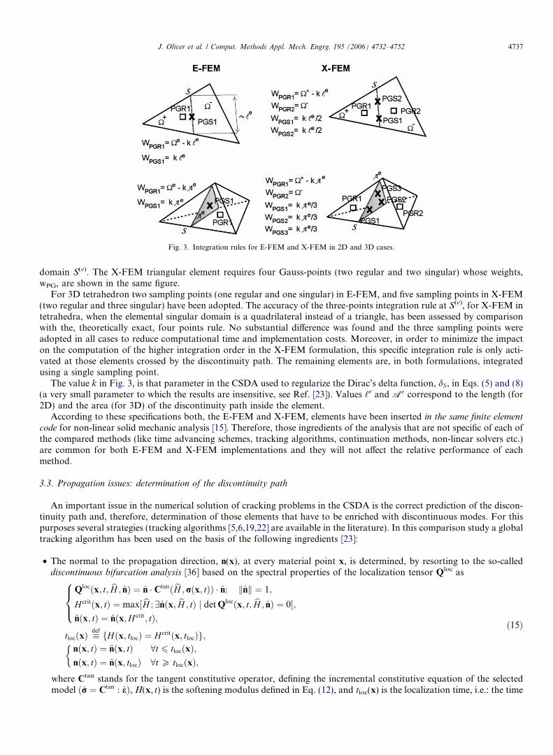
Fig. 3. Integration rules for E-FEM and X-FEM in 2D and 3D cases.


domain S(e). The X-FEM triangular element requires four Gauss-points (two regular and two singular) whose weights,wPG, are shown in the same figure.

For 3D tetrahedron two sampling points (one regular and one singular) in E-FEM, and five sampling points in X-FEM(two regular and three singular) have been adopted. The accuracy of the three-points integration rule at S(e), for X-FEM intetrahedra, when the elemental singular domain is a quadrilateral instead of a triangle, has been assessed by comparisonwith the, theoretically exact, four points rule. No substantial difference was found and the three sampling points wereadopted in all cases to reduce computational time and implementation costs. Moreover, in order to minimize the impacton the computation of the higher integration order in the X-FEM formulation, this specific integration rule is only acti-vated at those elements crossed by the discontinuity path. The remaining elements are, in both formulations, integratedusing a single sampling point.

The value k in Fig. 3, is that parameter in the CSDA used to regularize the Dirac’s delta function, dS, in Eqs. (5) and (8)(a very small parameter to which the results are insensitive, see Ref. [23]). Values ‘e and Ae correspond to the length (for2D) and the area (for 3D) of the discontinuity path inside the element.

According to these specifications both, the E-FEM and X-FEM, elements have been inserted in the same finite element

code for non-linear solid mechanic analysis [15]. Therefore, those ingredients of the analysis that are not specific of each ofthe compared methods (like time advancing schemes, tracking algorithms, continuation methods, non-linear solvers etc.)are common for both E-FEM and X-FEM implementations and they will not affect the relative performance of eachmethod.

3.3. Propagation issues: determination of the discontinuity path

An important issue in the numerical solution of cracking problems in the CSDA is the correct prediction of the discon-tinuity path and, therefore, determination of those elements that have to be enriched with discontinuous modes. For thispurposes several strategies (tracking algorithms [5,6,19,22] are available in the literature). In this comparison study a globaltracking algorithm has been used on the basis of the following ingredients [23]:

• The normal to the propagation direction, n(x), at every material point x, is determined, by resorting to the so-calleddiscontinuous bifurcation analysis [36] based on the spectral properties of the localization tensor Qloc as

Qlocðx; t; bH ; nÞ ¼ n � Ctanð bH ; rðx; tÞÞ � n; knk ¼ 1;

H critðx; tÞ ¼ max½ bH ; 9nðx; bH ; tÞ j det Qlocðx; t; bH ; nÞ ¼ 0�;~nðx; tÞ ¼ nðx;H crit; tÞ;

8><>:tlocðxÞ �

def fHðx; tlocÞ ¼ H critðx; tlocÞg;nðx; tÞ ¼ ~nðx; tÞ 8t 6 tlocðxÞ;nðx; tÞ ¼ ~nðx; tlocÞ 8t P tlocðxÞ;

�ð15Þ

where Ctan stands for the tangent constitutive operator, defining the incremental constitutive equation of the selectedmodel ð _r ¼ Ctan : _eÞ, H(x, t) is the softening modulus defined in Eq. (12), and tloc(x) is the localization time, i.e.: the time


as the chosen constitutive model becomes unstable allowing local bifurcation of the strain field and the formation of aweak discontinuity. It is characterized by the loss of positive definiteness of the localization tensor Qloc in Eq. (15).Closed form formulas for determination of n, for several families of constitutive models, can be found elsewhere[23,31,36]. The value of n(x, t) is computed for every material point (the single elemental sampling point for numericalpurposes) at every time step and it is frozen after the localization time, tloc, of the element.

• Construction, at every time step, of the enveloping family (lines in 2D or surfaces in 3D) of the vector field orthogonal ton(x, t) i.e.: the propagation vector field. This is done through a so-called pseudo-thermal algorithm (more details can befound in [22]). Then, those elements crossed by the same member (envelop) of that family and fulfilling the localizationcondition (t(x) P tloc(x)) are enriched with the discontinuous modes according to the respective E-FEM and X-FEMprocedures.

3.4. Robustness issues. Implicit–explicit time integration scheme

It is a very well-known fact the lack of robustness typical of models involving strain softening in computational materialfailure. Even as the B.V.P. is mathematically well posed, the loss of the positive definite character of the tangent constitu-tive operator progressively deteriorates the algorithmic stiffness of the problem, as material failure propagates through thefinite element mesh. As a consequence, the robustness of the convergence procedure for solving the non-linear problem isstrongly affected and, in most cases, convergence can be achieved only by using very skilful procedures, which translate intolarge computational costs. In order to overcome this problem, an implicit/explicit integration scheme, presented elsewhere[24,25], for integration of the constitutive model has been adopted for both the E-FEM and X-FEM procedures. Two arethe main advantages of that scheme:

• The resulting algorithmic tangent operator is always positive definite, which avoids the fundamental reasons for loss ofrobustness (at the cost of introducing an additional time-integration error in comparison with the standard implicit inte-gration scheme). In consequence, a result is always obtained whatever is the length of the time step. The accuracy of theresults can be then increased, and controlled, by shortening the length of the time step.

• The resulting algorithmic tangent operator is constant (for the adopted infinitesimal strain format) inside the time step. Inconsequence, convergence of the iteration procedure, to balance the internal and external forces, is achieved in just oneiteration per time step.

The beneficial effects of that integration procedure in computations involving strain softening are dramatic, both inrobustness and computational costs, as compared with the ones of the implicit scheme [24]. This is why, in the spirit, ofusing the best available algorithmic procedures in the comparison setting, the implicit/explicit integration scheme has beenadopted in this study for both the computations using E-FEM and X-FEM. In addition, and since robustness is almostcomplete, this guaranties the same number of time steps (and, therefore, of iterations) required to trace the response ofa given problem with both methods, and makes the comparison completely objective in terms of accuracy and computa-tional cost.

4. Numerical tests

In the computational setting defined in Section 3, the relative performances of the E-FEM vs. the X-FEM formulationsare compared by solving a set of two- and three-dimensional material failure problems in concrete, for single or multiplecrack cases. The following questions are aimed at being answered through this comparison:

• When applied to the same problem, do E-FEM and X-FEM provide the same (qualitative and quantitative) results?• How do both formulations compare in terms of accuracy?• What is their convergence rate with mesh refinement?• What is their relative computational cost?

All the examples shown below have been run in a standard PC equipped with a single Pentium 4 – 3.0 GHz, 512 MB Ram –processor. As for comparison of the computational cost in the tables below, the following nomenclature has been adoptedto identify some of the features and results for every problem:

• Nstep: number of time steps used for the complete analysis.• Nei: number of initial equations (at the beginning of the analysis without any enriching degree of freedom).• Nef: number of final equations (at the end of the analysis, including the additional enriching degrees of freedom).• RNe: ratio of number of equations Nef/Nei.


• bwi: initial average half bandwidth of the stiffness matrix.• bwf: final average half bandwidth of the stiffness matrix.• Rbw: ratio of average bandwidths bwf/bwi.• Ta: absolute CPU time for the problem (in seconds) for each formulation.• RCC: relative computational cost (Ta with X-FEM/Ta with E-FEM).

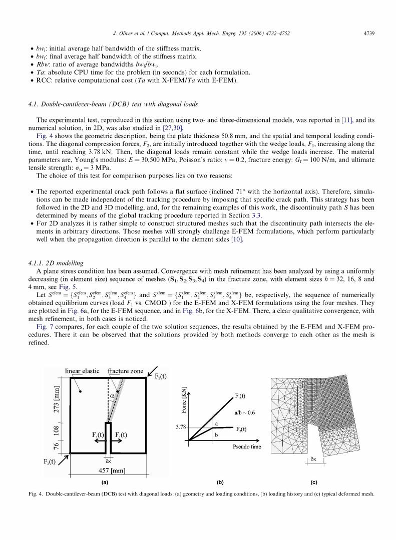
4.1. Double-cantilever-beam (DCB) test with diagonal loads

The experimental test, reproduced in this section using two- and three-dimensional models, was reported in [11], and itsnumerical solution, in 2D, was also studied in [27,30].

Fig. 4 shows the geometric description, being the plate thickness 50.8 mm, and the spatial and temporal loading condi-tions. The diagonal compression forces, F2, are initially introduced together with the wedge loads, F1, increasing along thetime, until reaching 3.78 kN. Then, the diagonal loads remain constant while the wedge loads increase. The materialparameters are, Young’s modulus: E = 30,500 MPa, Poisson’s ratio: m = 0.2, fracture energy: Gf = 100 N/m, and ultimatetensile strength: ru = 3 MPa.

The choice of this test for comparison purposes lies on two reasons:

• The reported experimental crack path follows a flat surface (inclined 71� with the horizontal axis). Therefore, simula-tions can be made independent of the tracking procedure by imposing that specific crack path. This strategy has beenfollowed in the 2D and 3D modelling, and, for the remaining examples of this work, the discontinuity path S has beendetermined by means of the global tracking procedure reported in Section 3.3.

• For 2D analyzes it is rather simple to construct structured meshes such that the discontinuity path intersects the ele-ments in arbitrary directions. Those meshes will strongly challenge E-FEM formulations, which perform particularlywell when the propagation direction is parallel to the element sides [10].

4.1.1. 2D modelling

A plane stress condition has been assumed. Convergence with mesh refinement has been analyzed by using a uniformlydecreasing (in element size) sequence of meshes (S1,S2,S3,S4) in the fracture zone, with element sizes h = 32, 16, 8 and4 mm, see Fig. 5.

Let Sefem ¼ fSefem1 ; Sefem

2 ; Sefem3 ; Sefem

4 g and Sxfem ¼ fSxfem1 ; Sxfem

2 ; Sxfem3 ; Sxfem

4 g be, respectively, the sequence of numericallyobtained equilibrium curves (load F1 vs. CMOD ) for the E-FEM and X-FEM formulations using the four meshes. Theyare plotted in Fig. 6a, for the E-FEM sequence, and in Fig. 6b, for the X-FEM. There, a clear qualitative convergence, withmesh refinement, in both cases is noticed.

Fig. 7 compares, for each couple of the two solution sequences, the results obtained by the E-FEM and X-FEM pro-cedures. There it can be observed that the solutions provided by both methods converge to each other as the mesh isrefined.

Fig. 4. Double-cantilever-beam (DCB) test with diagonal loads: (a) geometry and loading conditions, (b) loading history and (c) typical deformed mesh.

Fig. 5. 2D double-cantilever-beam (DCB) test with diagonal loads. Structured mesh sequence (S1,S2,S3,S4).

Fig. 6. 2D double-cantilever-beam (DCB) test with diagonal loads. Equilibrium curves (load F1 vs. CMOD): (a) E-FEM and (b) X-FEM solutions.


However, in order to translate these qualitative observations into figures, L2-norms of the differences are computed bymeans of the following formula:

keCMODikL2¼kSi � SrefkL2

kSrefkL2

¼

ffiffiffiffiffiffiffiffiffiffiffiffiffiffiffiffiffiffiffiffiffiffiffiffiffiffiffiffiffiffiffiffiffiffiffiffiffiffiffiffiffiffiffiffiffiffiffiffiffiffiffiZ maxðCMODÞ

0

ðSi � SrefÞ2 dx

sffiffiffiffiffiffiffiffiffiffiffiffiffiffiffiffiffiffiffiffiffiffiffiffiffiffiffiffiffiffiffiffiffiffiffiffiffiffiffiffiffiffiZ maxðCMODÞ

0

ðSrefÞ2 dx

s ; i ¼ 1; 2; 3; ð16Þ

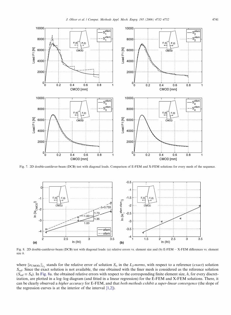
Fig. 7. 2D double-cantilever-beam (DCB) test with diagonal loads. Comparison of E-FEM and X-FEM solutions for every mesh of the sequence.

Fig. 8. 2D double-cantilever-beam (DCB) test with diagonal loads: (a) relative errors vs. element size and (b) E-FEM � X-FEM differences vs. elementsize h.


where keCMODikL2stands for the relative error of solution Si, in the L2-norms, with respect to a reference (exact) solution

Sref. Since the exact solution is not available, the one obtained with the finer mesh is considered as the reference solution(Sref � S4). In Fig. 8a. the obtained relative errors with respect to the corresponding finite element size, h, for every discret-ization, are plotted in a log–log diagram (and fitted in a linear regression) for the E-FEM and X-FEM solutions. There, itcan be clearly observed a higher accuracy for E-FEM, and that both methods exhibit a super-linear convergence (the slope ofthe regression curves is at the interior of the interval [1,2]).


The L2-norm of the difference of solutions in the two sequences of solutions Sefem ¼ fSefem1 ; Sefem

2 ; Sefem3 ; Sefem

4 g andSxfem ¼ fSxfem

1 ; Sxfem2 ; Sxfem

3 ; Sxfem4 g is obtained as

keefem�xfemi kL2

¼kSefem

i � Sxfemi kL2

kSxfemi kL2

¼

ffiffiffiffiffiffiffiffiffiffiffiffiffiffiffiffiffiffiffiffiffiffiffiffiffiffiffiffiffiffiffiffiffiffiffiffiffiffiffiffiffiffiffiffiffiffiffiffiffiffiffiffiffiffiffiffiffiffiffiZ maxðCMODÞ

0

ðSefemi � Sxfem

i Þ2 dx

sffiffiffiffiffiffiffiffiffiffiffiffiffiffiffiffiffiffiffiffiffiffiffiffiffiffiffiffiffiffiffiffiffiffiffiffiffiffiffiffiffiffiffiffiZ maxðCMODÞ

0

ðSxfemi Þ2 dx

s ; i ¼ 1; . . . ; 4; ð17Þ

where now keefem�xfemi kL2

is a measure of the difference of the solutions between the E-FEM and X-FEM procedures for thesame mesh. In Fig. 8b the corresponding results are plotted in a log–log diagram and fitted with a linear regression. Theclear reduction of the error with decreasing element size proves the convergence of both formulations, with mesh refinement,to the same value ðlimh!0ðSefem

i � Sxfemi Þ ¼ 0Þ.

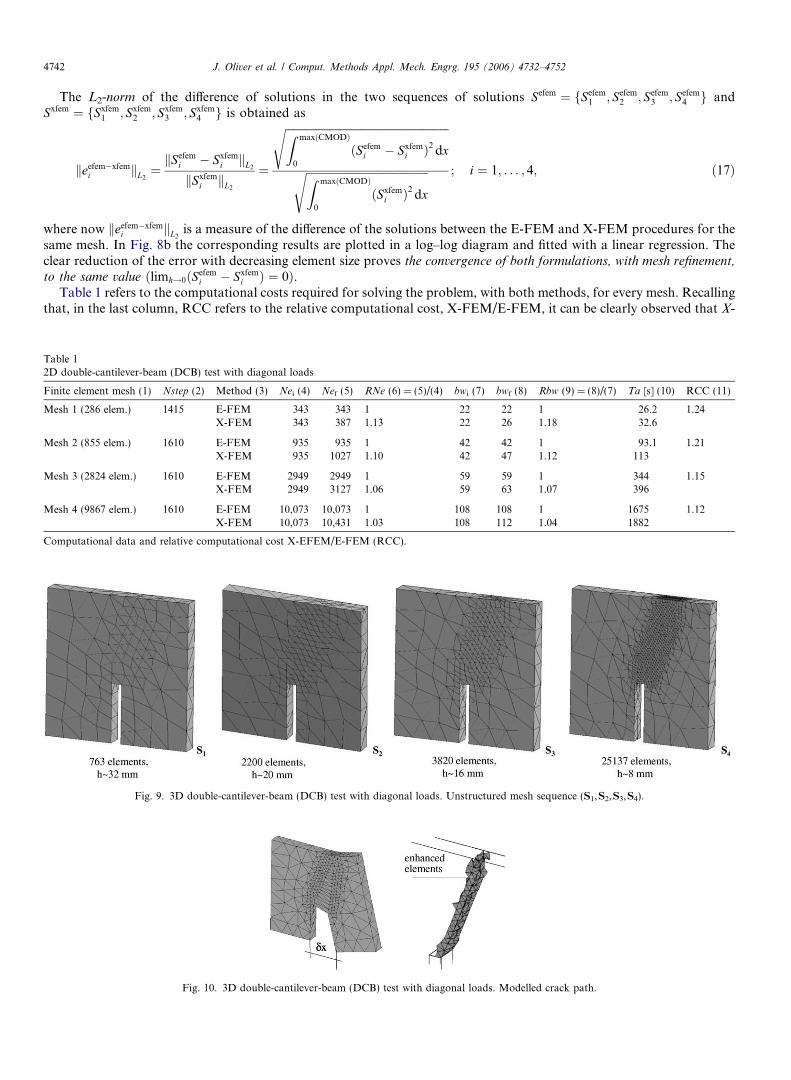
Table 1 refers to the computational costs required for solving the problem, with both methods, for every mesh. Recallingthat, in the last column, RCC refers to the relative computational cost, X-FEM/E-FEM, it can be clearly observed that X-

Fig. 9. 3D double-cantilever-beam (DCB) test with diagonal loads. Unstructured mesh sequence (S1,S2,S3,S4).

Fig. 10. 3D double-cantilever-beam (DCB) test with diagonal loads. Modelled crack path.

Table 12D double-cantilever-beam (DCB) test with diagonal loads

Finite element mesh (1) Nstep (2) Method (3) Nei (4) Nef (5) RNe (6) = (5)/(4) bwi (7) bwf (8) Rbw (9) = (8)/(7) Ta [s] (10) RCC (11)

Mesh 1 (286 elem.) 1415 E-FEM 343 343 1 22 22 1 26.2 1.24X-FEM 343 387 1.13 22 26 1.18 32.6

Mesh 2 (855 elem.) 1610 E-FEM 935 935 1 42 42 1 93.1 1.21X-FEM 935 1027 1.10 42 47 1.12 113

Mesh 3 (2824 elem.) 1610 E-FEM 2949 2949 1 59 59 1 344 1.15X-FEM 2949 3127 1.06 59 63 1.07 396

Mesh 4 (9867 elem.) 1610 E-FEM 10,073 10,073 1 108 108 1 1675 1.12X-FEM 10,073 10,431 1.03 108 112 1.04 1882

Computational data and relative computational cost X-EFEM/E-FEM (RCC).


FEM is, in all meshes, more expensive than E-FEM though the relative extra cost tends to decrease as the mesh is refined.This is the general trend observed in all the analyzed examples in this work.

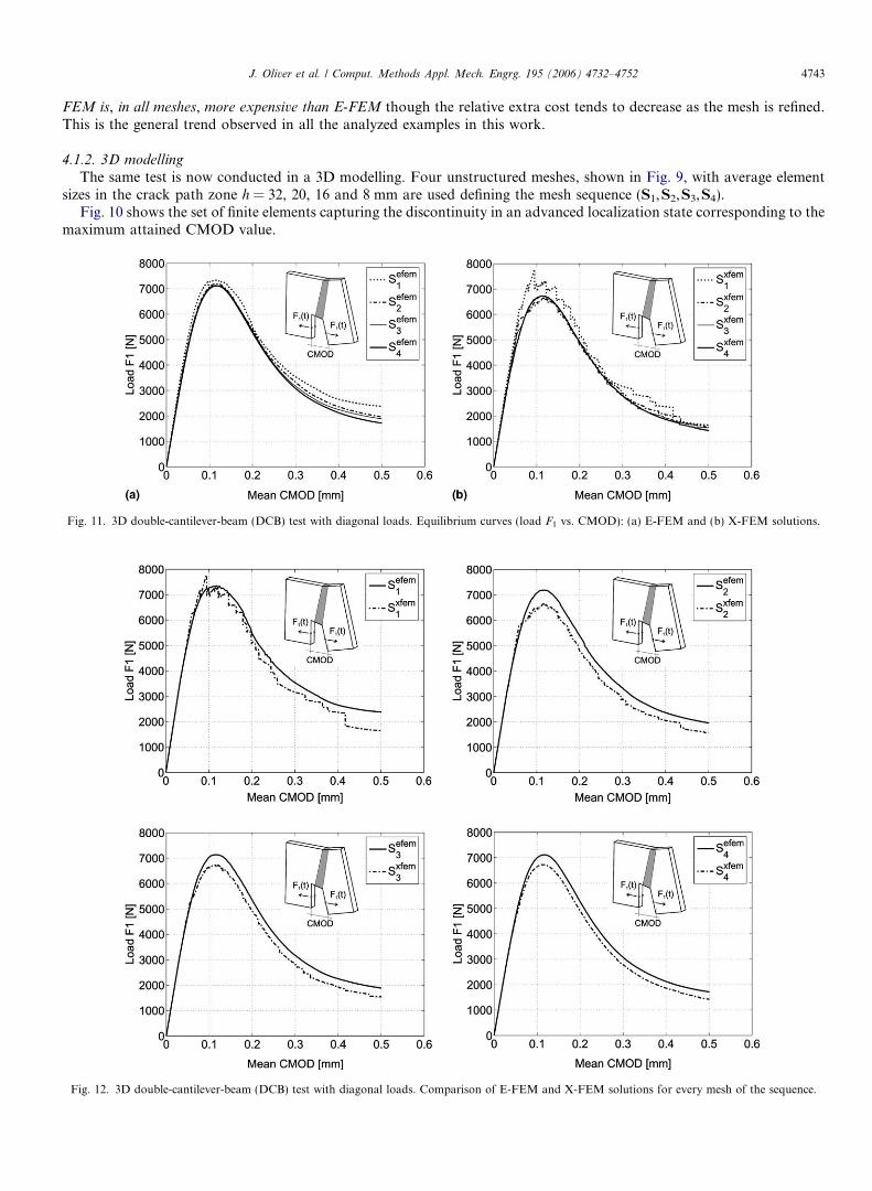
4.1.2. 3D modelling

The same test is now conducted in a 3D modelling. Four unstructured meshes, shown in Fig. 9, with average elementsizes in the crack path zone h = 32, 20, 16 and 8 mm are used defining the mesh sequence (S1,S2,S3,S4).

Fig. 10 shows the set of finite elements capturing the discontinuity in an advanced localization state corresponding to themaximum attained CMOD value.

Fig. 11. 3D double-cantilever-beam (DCB) test with diagonal loads. Equilibrium curves (load F1 vs. CMOD): (a) E-FEM and (b) X-FEM solutions.

Fig. 12. 3D double-cantilever-beam (DCB) test with diagonal loads. Comparison of E-FEM and X-FEM solutions for every mesh of the sequence.

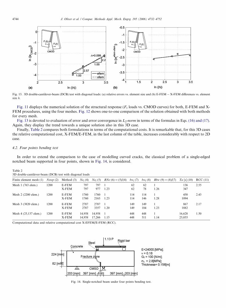
Fig. 13. 3D double-cantilever-beam (DCB) test with diagonal loads: (a) relative errors vs. element size and (b) E-FEM � X-FEM differences vs. elementsize h.


Fig. 11 displays the numerical solution of the structural response (F1 loads vs. CMOD curves) for both, E-FEM and X-FEM procedures, using the four meshes. Fig. 12 shows one-to-one comparison of the solution obtained with both methodsfor every mesh.

Fig. 13 is devoted to evaluation of error and error convergence in L2-norm in terms of the formulas in Eqs. (16) and (17).Again, they display the trend towards a unique solution also in this 3D case.

Finally, Table 2 compares both formulations in terms of the computational costs. It is remarkable that, for this 3D casesthe relative computational cost, X-FEM/E-FEM, in the last column of the table, increases considerably with respect to 2Dcase.

4.2. Four points bending test

In order to extend the comparison to the case of modelling curved cracks, the classical problem of a single-edgednotched beam supported in four points, shown in Fig. 14, is considered.

Table 23D double-cantilever-beam (DCB) test with diagonal loads





Mesh 4 (25,137 elem.) 1200 E-FEM 14,958 14,958 1 448 448 1 16,628 1.50X-FEM 14,958 17,266 1.15 448 511 1.14 25,055


Fig. 14. Single-notched beam under four points bending test.

Fig. 15. 2D four points bending test. Finite element meshes in the cracked zone and captured discontinuity paths with E-FEM and X-FEM enrichments.


The numerical simulations, for both two- and three-dimensional cases, have been done without imposing, beforehand,the discontinuity path, which is obtained using the methodology presented in Section 3.3.

4.2.1. 2D modelling

The four meshes, displayed in Fig. 15, are considered for the analyzes defining the sequences (S1,S2,S3,S4). Their aver-age element sizes in the fracture zone are, respectively, h = 32, 16, 8 and 4 mm. The same figure shows the obtained dis-continuity paths for both E-FEM and X-FEM enrichments (the elements crossed by the discontinuity path are shown indark). It can be checked as the captured discontinuity path tends to be the same as the mesh is refined. The solutionsequences Sefem ¼ fSefem

1 ; Sefem2 ; Sefem

3 ; Sefem4 g; Sxfem ¼ fSxfem

1 ; Sxfem2 ; Sxfem

3 ; Sxfem4 g for the structural responses, (load P vs. CMSD)

are plotted in Fig. 16 (for every enrichment in the complete mesh sequence) and in Fig. 17 (for both enrichments in thesame mesh of the sequence). Fig. 18 refers to the relative errors provided by E-FEM and X-FEM and the relative L2-norm

of the differences of solutions.Table 3 shows the comparative computational cost required for solving the different cases.

4.2.2. 3D modelling

The same problem is now solved using a 3D model and the four unstructured meshes of Fig. 19.In Fig. 20, 3D four points bending test details about the obtained three-dimensional curved crack surface are presented.Fig. 21 displays the sequences of solutions, with progressively refined meshes, supplied by the E-FEM and X-FEM

procedures. The abscissa (CSMD) has been computed as the average value of CSMD along the specimen thickness.

Fig. 16. 2D four points bending test. Load P vs. CMSD curves: (a) E-FEM and (b) X-FEM solutions.

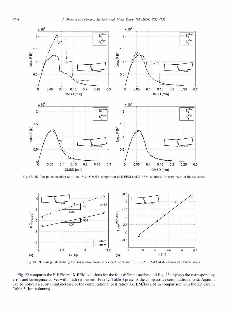
Fig. 17. 2D four points bending test. Load P vs. CMSD: comparison of E-FEM and X-FEM solutions for every mesh of the sequence.

Fig. 18. 2D four points bending test: (a) relative errors vs. element size h and (b) E-FEM � X-FEM differences vs. element size h.


Fig. 22 compares the E-FEM vs. X-FEM solutions for the four different meshes and Fig. 23 displays the correspondingerror and covergence curves with mesh refinement. Finally, Table 4 presents the comparative computational cost. Again itcan be noticed a substantial increase of the computational cost ratios X-FEM/E-FEM in comparison with the 2D case inTable 3 (last columns).

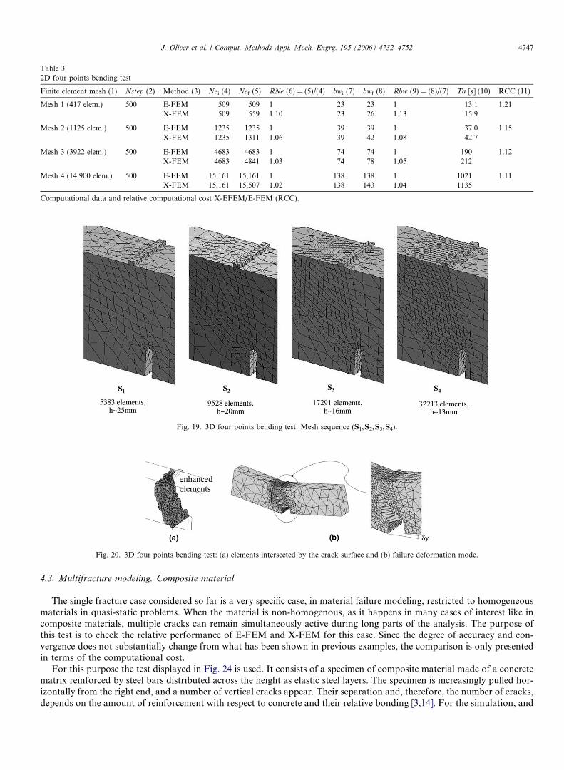
Table 32D four points bending test





Mesh 4 (14,900 elem.) 500 E-FEM 15,161 15,161 1 138 138 1 1021 1.11X-FEM 15,161 15,507 1.02 138 143 1.04 1135


Fig. 19. 3D four points bending test. Mesh sequence (S1,S2,S3,S4).

Fig. 20. 3D four points bending test: (a) elements intersected by the crack surface and (b) failure deformation mode.


4.3. Multifracture modeling. Composite material

The single fracture case considered so far is a very specific case, in material failure modeling, restricted to homogeneousmaterials in quasi-static problems. When the material is non-homogenous, as it happens in many cases of interest like incomposite materials, multiple cracks can remain simultaneously active during long parts of the analysis. The purpose ofthis test is to check the relative performance of E-FEM and X-FEM for this case. Since the degree of accuracy and con-vergence does not substantially change from what has been shown in previous examples, the comparison is only presentedin terms of the computational cost.

For this purpose the test displayed in Fig. 24 is used. It consists of a specimen of composite material made of a concretematrix reinforced by steel bars distributed across the height as elastic steel layers. The specimen is increasingly pulled hor-izontally from the right end, and a number of vertical cracks appear. Their separation and, therefore, the number of cracks,depends on the amount of reinforcement with respect to concrete and their relative bonding [3,14]. For the simulation, and

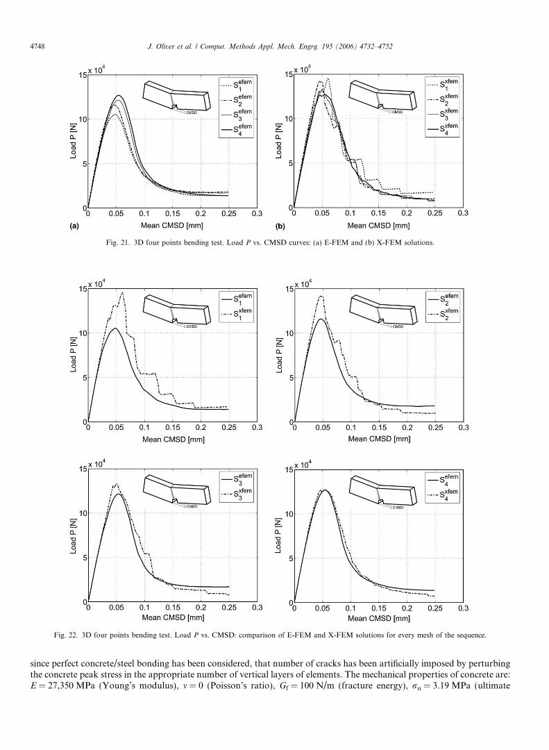
Fig. 21. 3D four points bending test. Load P vs. CMSD curves: (a) E-FEM and (b) X-FEM solutions.

Fig. 22. 3D four points bending test. Load P vs. CMSD: comparison of E-FEM and X-FEM solutions for every mesh of the sequence.


since perfect concrete/steel bonding has been considered, that number of cracks has been artificially imposed by perturbingthe concrete peak stress in the appropriate number of vertical layers of elements. The mechanical properties of concrete are:E = 27,350 MPa (Young’s modulus), m = 0 (Poisson’s ratio), Gf = 100 N/m (fracture energy), ru = 3.19 MPa (ultimate

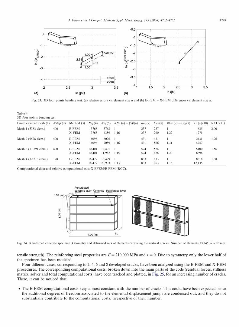
Fig. 23. 3D four points bending test: (a) relative errors vs. element size h and (b) E-FEM � X-FEM differences vs. element size h.

Table 43D four points bending test




Mesh 3 (17,291 elem.) 400 E-FEM 10,401 10,401 1 524 524 1 5400 1.56X-FEM 10,401 11,967 1.15 524 628 1.20 8398

Mesh 4 (32,213 elem.) 178 E-FEM 18,479 18,479 1 833 833 1 8818 1.38X-FEM 18,479 20,903 1.13 833 963 1.16 12,135


Fig. 24. Reinforced concrete specimen. Geometry and deformed sets of elements capturing the vertical cracks. Number of elements 23,245, h � 26 mm.


tensile strength). The reinforcing steel properties are E = 210,000 MPa and m = 0. Due to symmetry only the lower half ofthe specimen has been modeled.

Four different cases, corresponding to 2, 4, 6 and 8 developed cracks, have been analyzed using the E-FEM and X-FEMprocedures. The corresponding computational costs, broken down into the main parts of the code (residual forces, stiffnessmatrix, solver and total computational costs) have been tracked and plotted, in Fig. 25, for an increasing number of cracks.There, it can be noticed that

• The E-FEM computational costs keep almost constant with the number of cracks. This could have been expected, sincethe additional degrees of freedom associated to the elemental displacement jumps are condensed out, and they do notsubstantially contribute to the computational costs, irrespective of their number.

Fig. 25. Reinforced concrete plate. Computational CPU time as a function of the crack number for different parts of the simulation procedure: (a) residualevaluation and assembly; (b) stiffness matrix evaluation and assembly; (c) solving the linearized system of equations and (d) total computational cost.


• The X-FEM computational cost is always larger than the corresponding in E-FEM and grows linearly with the numberof modeled cracks. The most affected operations are the stiffness matrix construction and the solver (in turn the mosttime consuming operations). This should also be expected since the additional nodal degrees of freedom are not con-densed in this case.

• As a result, the relative computational cost X-FEM/E-FEM grows linearly with the number of modeled cracks.

5. Conclusions

Along this work a comparison of nodal (X-FEM) and elemental (E-FEM) enrichments in finite elements for capturingstrong discontinuities has been done. Both enrichments have been implemented in the same finite element code, on the basisof optimized algorithms and coding, and tested on a set of 2D and 3D examples under exactly the same conditions. Theobtained results can be summarized as follows:

• When implemented on the basis of the same element (linear triangles and linear tetrahedra in this study), both formu-

lations converge to the same results, either the qualitative (captured discontinuity paths) or the quantitative ones.• The rate of convergence of both enrichments is similar. Substantial differences in terms of convergence rates, in L2-norms,

have not been found (for both cases the convergence rates are fairly superior to linear).• Therefore, unlike what some times has been asserted, the different kind of interpolation of the displacement jump provided

by both types of enrichments (linear for X-FEM, element wise constant for E-FEM) does not affect neither the accuracy

of the representation of the discontinuity nor the convergence rate. Neither the fact that X-FEM, unlike E-FEM, allows

discontinuous elemental regular strains across the discontinuity interface seems to affect the accuracy and convergence rates.

They rather seem to be dependent on the degree of interpolation for the standard displacement modes of the chosenbasic element (linear in this study).

• It has been observed that, for rather coarse meshes, both the accuracy and the smoothness of the response are generallyhigher with the E-FEM formulation. More specifically: the response curves corresponding to X-FEM exhibit, as com-pared with those with E-FEM, a more abrupt shape and jumps that can be associated to the relative delay of the former in


the activation of the degrees of freedom of the enriching modes as a new element is crossed by the crack path. This effect,that can be also observed to a lesser extent in the E-FEM results, diminishes with the mesh refinement and also appearsin the results provided by other authors using X-FEM [9,35]. It has been reported the addition of new enriching modesat the crack tip [37] that might, at least partially, correct this response, but this type of techniques, that belong to ahigher level of sophistication and that are still under development [12], has not been applied here in none of the E-FEM and X-FEM formulations.

• Computational costs are, in all cases, favourable to the E-FEM enrichment. For single crack modelling X-FEM is 1.1–1.2times (in 2D cases) and 1.3–2.5 times (in 3D cases) more expensive than E-FEM. These ratios decrease with increasinglevels of discretizations. The reasons for the higher cost for X-FEM seem to be the additional, not condensable at ele-mental level, degrees of freedom and the higher order integration necessary in X-FEM. Certainly, those figures shouldbe taken as a trend, since they could be modified in any sense by alternative implementations. They correspond to thebest implementation knowledge of the authors, after a substantial coding effort in a reasonably well-checked finite ele-ment code.

• As for multiple cracking modelling, the computational costs associated to the E-FEM enrichment remain almost constantfor increasing number of cracks. On the contrary, for the X-FEM enrichment, the computational cost increases linearly

with the number of involved cracks. For the considered 3D case this increase is up to around 20% of the total costper every additional crack.

• In the context of the implicit/explicit integration of the constitutive model both formulations are very robust. All simulationshave been conducted beyond the critical loads and up to almost complete exhaustion of the loading capacity.

In summary, from the specific comparison setting devised for this study, based on standard formulations of both methods

and their optimized implementations and coding, the main differences are: (a) the higher relative computational cost of X-FEM with respect to E-FEM, associated to the possibility of condensation at elemental level in E-FEM and the higherintegration order in X-FEM, and (b) the higher accuracy in E-FEM, mainly for coarse meshes. Anyhow, both methodsare amenable to be reformulated and improved, which could define different scenarios for which the corresponding com-parison studies should be done.

Acknowledgements

Financial support from the Spanish Ministry of Science and Technology, through Grant BIA 2004-02080, and from theCatalan Government Research Department, through the CIRIT Grant 2001-SGR 00262, is gratefully acknowledged.

The third author was supported by the Programme Alban, the European Union Programme of High Level Scholarshipsfor Latin American, scholarship, Ref. No. E04D035536AR.

References

[1] J. Alfaiate, New developments in the study of strong embedded discontinuities infinite elements, Adv. Fract. Damage Mech. 251–252 (2003) 109–114.[2] F. Armero, K. Garikipati, An analysis of strong discontinuities in multiplicative finite strain plasticity and their relation with the numerical simulation

of strain localization in solids, Int. J. Solids Struct. 33 (1996) 2863–2885.[3] Z. Bazant, L. Cedolin, Fracture mechanics of reinforced concrete, J. Eng. Mech. Div. ASCE (1980) 1287–1305.[4] T. Belytschko, H. Chen, J.X. Xu, G. Zi, Dynamic crack propagation based on loss of hyperbolicity and a new discontinuous enrichment, Int. J.

Numer. Methods Engrg. 58 (2003) 1873–1905.[5] T. Belytschko, N. Moes, S. Usui, C. Parimi, Arbitrary discontinuities in finite elements, Int. J. Numer. Methods Engrg. 50 (2001) 993–1013.[6] C. Feist, G. Hofstetter, Computational aspects of concrete fracture simulations in the framework of the SDA. Presented at Fracture Mechanics of

Concrete Structures FRAMCOS 2004, Vale, Co, USA, 2004.[7] K. Garikipati, T.J.R. Hughes, A study of strain-localization in a multiple scale framework. The one dimensional problem, Comput. Methods Appl.

Mech. Engrg. 159 (1998) 193–222.[8] T.C. Gasser, G.A. Holzapfel, Geometrically non-linear and consistently linearized embedded strong discontinuity models for 3D problems with an

application to the dissection analysis of soft biological tissues, Comput. Methods Appl. Mech. Engrg. 192 (2003) 5059–5098.[9] T.C. Gasser, G.A. Holzapfel, Modeling 3D crack propagation in unreinforced concrete using PUFEM, Comput. Methods Appl. Mech. Engrg. 194

(2005) 2859–2896.[10] M. Jirasek, Comparative study on finite elements with embedded discontinuities, Comput. Methods Appl. Mech. Engrg. 188 (2000) 307–330.[11] A.S. Kobayashi, M.N. Hawkins, D.B. Barker, B.M. Liaw, Fracture process zone of concrete, in: S.S.P. (Ed.), Application of Fracture Mechanics to

Cementitious Composites, Marinus Nujhoff Publ., Dordrecht, 1985, pp. 25–50.[12] P. Laborde, J. Pommier, Y. Renard, M. Salaun, High order extended finite element method for cracked domains. Presented at Computational

Plasticity VIII: Fundamentals and Applications, Barcelona, Spain, 2005.[13] R. Larsson, K. Runesson, N.S. Ottosen, Discontinuous displacement approximation for capturing plastic localization, Int. J. Numer. Methods Engrg.

36 (1993) 2087–2105.[14] K. Liao, K.L. Reifsnider, A tensile strength model for unidirectional fiber-reinforced brittle matrix composite, Int. J. Fract. 106 (2000) 95–115.[15] M. Cervera, C. Agelet, M. Chiumenti, COMET: A Multipurpose Finite Element Code for Numerical Analysis in Solid Mechanics, Technical

University of Catalonia (UPC), 2001.


[16] S. Mariani, U. Perego, Extended finite element method for quasi-brittle fracture, Int. J. Numer. Methods Engrg. 58 (2003) 103–126.[17] N. Moes, N. Sukumar, B. Moran, T. Belytschko, An extended finite element method (X-FEM) for two and three-dimensional crack modelling.

Presented at ECCOMAS 2000, Barcelona, Spain, 2000.[18] J. Mosler, G. Meschke, 3D modelling of strong discontinuities in elastoplastic solids: fixed and rotating localization formulations, Int. J. Numer.

Methods Engrg. 57 (2003) 1553–1576.[19] J. Mosler, G. Meschke, Embedded crack vs. smeared crack models: a comparison of elementwise discontinuous crack path approaches with emphasis

on mesh bias, Comput. Methods Appl. Mech. Engrg. 193 (2004) 3351–3375.[20] J. Oliver, Modelling strong discontinuities in solid mechanics via strain softening constitutive equations. 2. Numerical simulation, Int. J. Numer.

Methods Engrg. 39 (1996) 3601–3623.[21] J. Oliver, On the discrete constitutive models induced by strong discontinuity kinematics and continuum constitutive equations, Int. J. Solids Struct.

37 (2000) 7207–7229.[22] J. Oliver, A.E. Huespe, Continuum approach to material failure in strong discontinuity settings, Comput. Methods Appl. Mech. Engrg. 193 (2004)

3195–3220.[23] J. Oliver, A.E. Huespe, Theoretical and computational issues in modelling material failure in strong discontinuity scenarios, Comput. Methods Appl.

Mech. Engrg. 193 (2004) 2987–3014.[24] J. Oliver, A.E. Huespe, S. Blanco, D.L. Linero, Stability and robustness issues in numerical modeling of material failure in the strong discontinuity

approach, Comput. Methods Appl. Mech. Engrg. accepted for publication.[25] J. Oliver, A.E. Huespe, M.D.G. Pulido, S. Blanco, Recent advances in computational modelling of material failure. Presented at 4th European

Congress on Computational Methods in Applied Sciences and Engineering (ECCOMAS 2004), University of Jyvaskyla, Jyvaskyla, Finland, 2004.[26] J. Oliver, A.E. Huespe, M.D.G. Pulido, S. Blanco, D. Linero, New developments in computational material failure mechanics. Presented at Sixth

World Congress on Computational Mechanics (WCCM VI), Beijing, PR China, 2004.[27] J. Oliver, A.E. Huespe, M.D.G. Pulido, E. Chaves, From continuum mechanics to fracture mechanics: the strong discontinuity approach, Engrg.

Fract. Mech. 69 (2002) 113–136.[28] J. Oliver, A.E. Huespe, E. Samaniego, A study on finite elements for capturing strong discontinuities, Int. J. Numer. Methods Engrg. 56 (2003) 2135–

2161.[29] R.L. Borja, R.A. Regueiro, A finite element model for strain localization analysis of strongly discontinuous fields based on standard Galerkin

approximation, Comput. Methods Appl. Mech. Engrg. (2000) 1529–1549.[30] J.G. Rots, Computational Modeling of Concrete Fractures, Delft University of Technology, 1988.[31] K. Runesson, Z. Mroz, A note on nonassociated plastic flow rules, Int. J. Plast. 5 (1989) 639–658.[32] J. Simo, J. Oliver, F. Armero, An analysis of strong discontinuities induced by strain-softening in rate-independent inelastic solids, Comput. Mech.

12 (1993) 277–296.[33] A. Simone, Partition of unity-based discontinuous elements for interface phenomena: computational issues, Commun. Numer. Methods Engrg.

20 (2004) 465–478.[34] B.W. Spencer, P.B. Shing, Rigid-plastic interface for an embedded crack, Int. J. Numer. Methods Engrg. 56 (2003) 2163–2182.[35] G.N. Wells, L.J. Sluys, A new method for modelling cohesive cracks using finite elements, Int. J. Numer. Methods Engrg. 50 (2001) 2667–2682.[36] K. Willam, N. Sobh, Bifurcation analysis of tangential material operators, in: G.N. Pande, J. Middleton (Eds.), Transient/Dynamic Analysis and

Constitutive Laws for Engineering Materials, vol. 2, Martinus-Nijhoff Publishers, 1987, pp. C4/1–C4/13.[37] G. Zi, T. Belytschko, New crack-tip elements for XFEM and applications to cohesive cracks, Int. J. Numer. Methods Engrg. 57 (2003) 2221–2240.

Documents

A comparative study on ﬁnite elements for capturing strong ... J., A... · A comparative study on ﬁnite elements for capturing strong discontinuities: E-FEM vs X-FEM J. Oliver