Open Journal of Civil Engineering, 2017, 7, 539-552 http://www.scirp.org/journal/ojce

ISSN Online: 2164-3172 ISSN Print: 2164-3164

DOI: 10.4236/ojce.2017.74036 Dec. 7, 2017 539 Open Journal of Civil Engineering

A Comparison among Manual and Automatic Calibration Methods in VISSIM in an Expressway (Chihuahua, Mexico)

Daphne Espejel-Garcia1, Jose Alejandro Saniger-Alba2, Gilberto Wenglas-Lara1, Vanessa Veronica Espejel-Garcia1, Alejandro Villalobos-Aragon1

1Facultad de Ingenieria, Universidad Autonoma de Chihuahua, Chihuahua, Mexico 2PTV Group Mexico, Ciudad de Mexico, Mexico

Abstract Traffic microsimulation is an essential tool in urban transportation and road planning. Its calibration is essential to attain representative results validated with real-world conditions. VISSIM (Verkehr in Städten—SIMulationsmodell) oper-ates with the Wiedemann’s psycho-physical car-following model for freeway travel that considers safety distances (standstill and movement) during simu-lation. Calibration in this paper was achieved by using two different ap-proaches: a) manual and b) genetic algorithm (with the GEH statistic formula) calibration techniques. Calibration and validation of this model were per-formed at the Periferico de la Juventud expressway in Chihuahua City, in northern Mexico. The Periferico de la Juventud (PDJ) has a N-S orientation and a length of ca. 20 km, with its northern section being its most congested portion. Its highest vehicle volume occurs at noon, with 3700 vehicles per hour, with 95% being passenger cars and the other 5% heavy goods vehicles. PDJ’s speed limit is 70 km∙h−1, but the driver’s behavior has a tendency to-wards the aggressive performance. A total of 82 standstill and 82 look-ahead distances were obtained from unmanned aerial vehicles (UAV) images, with values ranging from 0.8 to 4.7 m and from 0.2 to 28 m, respectively. VISSIM calibrated parameter values were calculated for this expressway, being slightly above than the VISSIM default ones; and was validated with travel times and look-ahead distances. Results contribute information for the city’s future in-stallment of public transportation systems, and should help decision makers deal with future urban planning.

Keywords VISSIM, Genetic Algorithm Calibration, Expressway, Chihuahua

How to cite this paper: Espejel-Garcia, D., Saniger-Alba, J.A., Wenglas-Lara, G., Espe-jel-Garcia, V.V. and Villalobos-Aragon, A. (2017) A Comparison among Manual and Automatic Calibration Methods in VISSIM in an Expressway (Chihuahua, Mexico). Open Journal of Civil Engineering, 7, 539-552. https://doi.org/10.4236/ojce.2017.74036 Received: October 16, 2017 Accepted: December 4, 2017 Published: December 7, 2017 Copyright © 2017 by authors and Scientific Research Publishing Inc. This work is licensed under the Creative Commons Attribution International License (CC BY 4.0). http://creativecommons.org/licenses/by/4.0/

Open Access

D. Espejel-Garcia et al.

DOI: 10.4236/ojce.2017.74036 540 Open Journal of Civil Engineering

1. Introduction

Traffic microsimulation is the main traffic analysis method used to solve trans-portation issues. Simulation models provide analyzed traffic data under distinct conditions at low cost [1]. VISSIM (Verkehr in Städten—SIMulationsmodell developed by the German company Planung Transport Verkehr, PTV) is one of the most popular traffic flow microsimulation softwares due to its modelling based on the interactions among pedestrians, vehicles, heavy goods vehicles (HGV) and any other type of transportation [2] [3], which also analyses and op-timizes traffic flow in detail [4]. VISSIM employs the car following model for freeway travel that accounts the Wiedemann model [5] [6] and consider differ-ent aspects such as free driving, approaching, following, and braking [3] [7].

Transportation and its environmental impact, as well as mobility, are two of the most important factors considered in urban economy and quality of life [8]. Hence traffic simulation is crucial for transportation and road planning [4]. Ca-libration of certain parameters is needed to evaluate traffic and planning opera-tions and applications, being critical for obtaining realistic microsimulation re-sults [9]. Calibration is essential to obtain reliable results, along with the appro-priate data collecting technique, which mostly depends on cost and access [1]. Unmanned Aerial Vehicles (UAV or drones) images represent a low cost and accessible method to capture vehicle operations over time [1]. Several techniques have been used to improve calibration in VISSIM. Occasionally, the parameter configuration (such as average standstill distance and additive part of safety dis-tance) should be determined for one location, due to the area’s distinct characte-ristics. Without proper calibration, the simulated traffic outcome does not coin-cide with real-world settings, and microsimulation models cannot help analysts to solve any traffic issue [1].

Several methods have been developed to calibrate traffic microsimulation pa-rameters, and can be divided in manual and automated [10]. Although the ma-nual technique is broadly used due to its precision without dealing with compli-cated computer coding [10], it is generally considered as a time-consuming me-thod. Many authors have attempted and successfully developed computerized calibration methods (e.g. [11] [12] [13] [14] [15]) using different types of algo-rithms, such as genetic algorithm (GA), evolutionary algorithm (EA), Neld-er-Mead algorithm (NMA), sensitivity analysis method (SA), pareto archived dynamically dimensioned search (PA-DDS), and particle swarm optimization (PSO) [16], but they are still time consuming due to the large number of itera-tions, and are difficult to use due to their inherent complexity.

This project compares the manual method outcomes with those resulting from the use of a relatively simpler calibration method: an application of the GEH statistics formula within VISSIM’s software through a genetic algorithm (GA). It is now possible to link a programming software (e.g. Matlab, used in this paper) containing both the GA code and the GEH equation within VISSIM, making it possible to calibrate parameters in a shorter amount of time. Though

D. Espejel-Garcia et al.

DOI: 10.4236/ojce.2017.74036 541 Open Journal of Civil Engineering

the manual method is still widely accepted and employed by traffic analysts, the automatic technique offers its accuracy and it takes less time, once the correct equation is selected and executed.

2. Scope and Purpose

This project provides road data (such as flow and vehicular classification, speeds, and flow capacity) of the most important expressway of Chihuahua city: Perife-rico de la Juventud (PDJ). This data is not currently available and previous records do not exist (as for most of roads in Chihuahua), making it difficult to model it over the years. Manual calibration is the main technique used in pre-vious work performed in the city. This paper uses the genetic algorithm method using the GEH statistic formula within VISSIM, allowing a comparison between both methods. Microscopic simulation of this roadway will allow users (and au-thorities) to visualize its current behavior, and future scenarios’ projection; as well as propose strategies to solve road congestions along its way.

2.1. Background

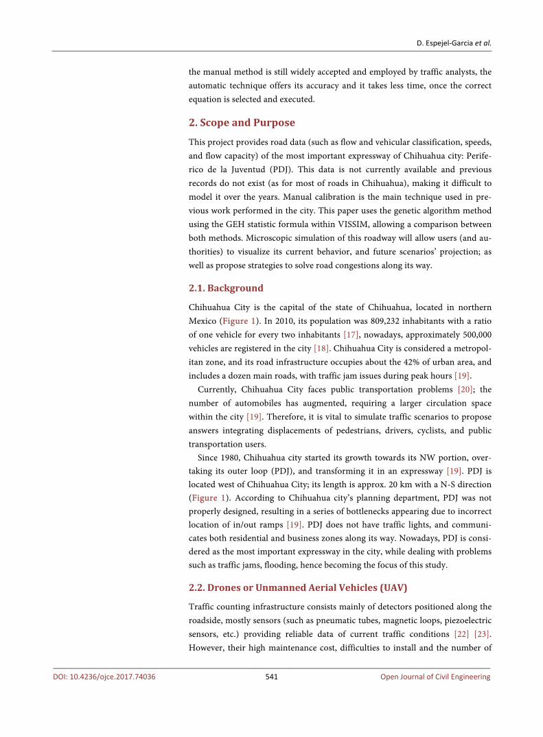
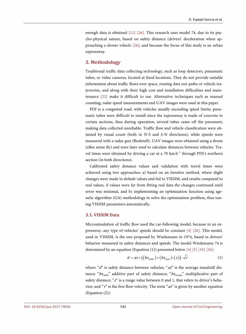
Chihuahua City is the capital of the state of Chihuahua, located in northern Mexico (Figure 1). In 2010, its population was 809,232 inhabitants with a ratio of one vehicle for every two inhabitants [17], nowadays, approximately 500,000 vehicles are registered in the city [18]. Chihuahua City is considered a metropol-itan zone, and its road infrastructure occupies about the 42% of urban area, and includes a dozen main roads, with traffic jam issues during peak hours [19].

Currently, Chihuahua City faces public transportation problems [20]; the number of automobiles has augmented, requiring a larger circulation space within the city [19]. Therefore, it is vital to simulate traffic scenarios to propose answers integrating displacements of pedestrians, drivers, cyclists, and public transportation users.

Since 1980, Chihuahua city started its growth towards its NW portion, over-taking its outer loop (PDJ), and transforming it in an expressway [19]. PDJ is located west of Chihuahua City; its length is approx. 20 km with a N-S direction (Figure 1). According to Chihuahua city’s planning department, PDJ was not properly designed, resulting in a series of bottlenecks appearing due to incorrect location of in/out ramps [19]. PDJ does not have traffic lights, and communi-cates both residential and business zones along its way. Nowadays, PDJ is consi-dered as the most important expressway in the city, while dealing with problems such as traffic jams, flooding, hence becoming the focus of this study.

2.2. Drones or Unmanned Aerial Vehicles (UAV)

Traffic counting infrastructure consists mainly of detectors positioned along the roadside, mostly sensors (such as pneumatic tubes, magnetic loops, piezoelectric sensors, etc.) providing reliable data of current traffic conditions [22] [23]. However, their high maintenance cost, difficulties to install and the number of

D. Espejel-Garcia et al.

DOI: 10.4236/ojce.2017.74036 542 Open Journal of Civil Engineering

Figure 1. Location map of the case study [21]. needed devices, limit the use of such technique [24]. In contrast, lower cost and flexible techniques controlled by remote observations, such as manual counts, infra-red readers, radar, video image detection, drones (or UAV), etc. are also used [1] [23].

A main issue while collecting traffic data for microsimulation modeling and calibration is its high cost. All the above has motivated researchers to look for more economical tools, such as the use of video and/or photographic images storing single vehicle operations over time, while offering valuable tools and data for calibration and validation of traffic models. UAV technologies were intro-duced for traffic surveillance and traffic parameters estimation [1] [25]. Drones have been used to perform traffic conditions analyses, because they provide high resolution georeferenced images at low costs and with short data collecting times, but there are also limiting factors, such as weather conditions, physical obstacles, battery life, and permission to fly certain areas, etc. [1] [25].

2.3. VISSIM Software

VISSIM is a traffic flow microsimulation software centered on traffic flow beha-vior and interactions between pedestrians with any type of vehicles [3]; and fo-cuses in analyses and optimization of traffic flow, to model in detailed real con-ditions [4]. VISSIM works with four different vehicles’ behavior models [26]: a) car-following; b) lane changes; c) lateral behavior; and d) reaction to the amber signal light. The car-following model is the one that recreates the better the con-ditions of an expressway (i.e. PDJ), and defines saturation flow. VISSIM operates with a model developed by Wiedemann [5] [6], and has two versions: a) 74, used for urban traffic and merging areas, works with only three parameters (average standstill distance, additive part of safety distance, and multiplicative part of safety distance), and b) 99, used for highways and freeways with no merging areas, which deals with nine parameters (standstill distance, headway time, and seven other parameters related to deceleration), and allows a finer calibration if

D. Espejel-Garcia et al.

DOI: 10.4236/ojce.2017.74036 543 Open Journal of Civil Engineering

enough data is obtained [12] [26]. This research uses model 74, due to its psy-cho-physical nature, based on safety distance (drivers’ deceleration when ap-proaching a slower vehicle [26]; and because the focus of this study is an urban expressway.

3. Methodology

Traditional traffic data collecting technology, such as loop detectors, pneumatic tubes, or video cameras, located at fixed locations. They do not provide suitable information about traffic flows over space, routing data nor paths or vehicle tra-jectories, and along with their high cost and installation difficulties and main-tenance [22] make it difficult to use. Alternative techniques such as manual counting, radar speed measurements and UAV images were used in this paper.

PDJ is a congested road, with vehicles usually exceeding speed limits; pneu-matic tubes were difficult to install since the expressway is made of concrete in certain sections, thus during operation, several tubes came off the pavement; making data collected unreliable. Traffic flow and vehicle classification were ob-tained by visual count (both in N-S and S-N directions), while speeds were measured with a radar gun (Bushnell). UAV images were obtained using a drone (eBee sense fly) and were later used to calculate distances between vehicles. Tra-vel times were obtained by driving a car at a 70 km∙h−1 through PDJ’s northern section (in both directions).

Calibrated safety distance values and validation with travel times were achieved using two approaches: a) based on an iterative method, where slight changes were made to default values and fed to VISSIM, and results compared to real values, if values were far from fitting real data the changes continued until error was minimal, and b) implementing an optimization function using age-netic algorithm (GA) methodology to solve the optimization problem, thus tun-ing VISSIM parameters automatically.

3.1. VISSIM Data

Microsimulation of traffic flow used the car-following model, because in an ex-pressway, any type of vehicles’ speeds should be constant [4] [26]. This model, used in VISSIM, is the one proposed by Wiedemann in 1974, based in drivers’ behavior measured in safety distances and speeds. The model Wiedemann 74 is determined by an equation (Equation (1)) presented below [4] [5] [10] [26]:

( ) ( ) ( )( )addit multd ax bx bx z v= + + ⋅ ⋅ (1)

where “d” is safety distance between vehicles; “ax” is the average standstill dis-tance; “bxaddit” additive part of safety distance; “bxmultip” multiplicative part of safety distance; “z” is a range value between 0 and 1, that refers to driver’s beha-vior; and “v” is the free flow velocity. The term “ax” is given by another equation (Equation (2)):

D. Espejel-Garcia et al.

DOI: 10.4236/ojce.2017.74036 544 Open Journal of Civil Engineering

1 1n add n multipax L ax RND ax−= + + ∗ (2)

where “Ln−1” is the vehicle length; “axadd and axmultip” are calibration parameters and “RND1n” is normal distribution of random vehicles’ number.

A road network was created in VISSIM based on Bing maps satellite images, and PDJ’s lane widths were verified in situ (3.5 m), only for its northern section, because it is also its busiest part.

3.2. Safety Distance

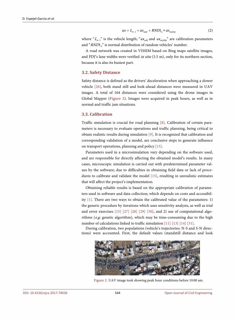
Safety distance is defined as the drivers’ deceleration when approaching a slower vehicle [26], both stand still and look-ahead distances were measured in UAV images. A total of 164 distances were considered using the drone images in Global Mapper (Figure 2). Images were acquired in peak hours, as well as in normal and traffic jam situations.

3.3. Calibration

Traffic simulation is crucial for road planning [8]. Calibration of certain para-meters is necessary to evaluate operations and traffic planning, being critical to obtain realistic results during simulation [9]. It is recognized that calibration and corresponding validation of a model, are conclusive steps to generate influence on transport operations, planning and policy [15].

Parameters used in a microsimulation vary depending on the software used, and are responsible for directly affecting the obtained model’s results. In many cases, microscopic simulation is carried out with predetermined parameter val-ues by the software; due to difficulties in obtaining field data or lack of proce-dures to calibrate and validate the model [15], resulting in unrealistic estimates that will affect the project’s implementation.

Obtaining reliable results is based on the appropriate calibration of parame-ters used in software and data collection; which depends on costs and accessibil-ity [1]. There are two ways to obtain the calibrated value of the parameters: 1) the generic procedure by iterations which uses sensitivity analysis, as well as trial and error exercises [15] [27] [28] [29] [30], and 2) use of computational algo-rithms (e.g. genetic algorithm), which may be time-consuming due to the high number of calculations linked to traffic simulation [11] [13] [14] [31].

During calibration, two populations (vehicle’s trajectories: N-S and S-N direc-tions) were accounted. First, the default values (standstill distance and look

Figure 2. UAV image took showing peak hour conditions before 10:00 am.

D. Espejel-Garcia et al.

DOI: 10.4236/ojce.2017.74036 545 Open Journal of Civil Engineering

ahead distance) in VISSIM were used, but the results were different from the ones obtained in the field. Slight changes of increments of 0.1 in these default parameters later were fed to VISSIM in an iterative way. Calibrated values were validated using real travel times and look ahead distances, and comparing them to the simulated times.

In the GA, through Matlab, the code was adapted, using the examples of ob-jective functions (GEH statistics) [32] [33] [34]. In the Geoffrey E. Havers GEH function (Equation (3)) [34], data obtained in the field was integrated and the comparison with the simulated data in VISSIM was performed, so that the error could be reduced, and the calibrated parameters could be obtained:

( )( )

22 M CGEH

M C∗ −

=+

(3)

It is possible to link Matlab with VISSIM through a COM library, which al-lows the extraction of information from the simulations to be considered in GA iterations. In the same way, as in the iterative analysis, the parameters bxadd and bxmult were calibrated, so that the particles were optimized within a wide range of data, and the most appropriate selected.

4. Results 4.1. Vehicle Capacity and Speeds

PDJ is a N-S expressway with long lasting traffic jams at peak hours throughout the day. Its highest traffic flow occurs from the north to south direction. Vehicle count was measured at its northern section, from its north entrance at its inter-section with Homero Avenue, all the way to its southern entrance where it joins Cantera Avenue, almost 8.5 km in length. The highest vehicle volume occurs at noon, reaching almost 3700 vehicles per hour (Table 1). The visual count al-lowed a vehicle type classification, with 95% being passenger cars and the re-maining 5%, distributed between heavy goods vehicles (HGV) with different axes number.

PDJ’s speed limit is 70 km∙h−1, but the driver’s behavior has a tendency to-wards the aggressive performance. Radar speeds ranged from 40 to 120 km∙h−1, and from a total of 2244 measurements, the average speed was 67.75 km∙h−1.

4.2. Safety Distance

A total of 82 standstill and 82 look-ahead distances were obtained from UAV images, with values ranging from 0.8 to 4.7 m and from 0.2 to 28 m, respectively. Travel times were obtained as described in the methodology section.

4.3. Calibration and Validation

Manual calibration parameter values were acquired performing several simula-tions in VISSIM, by changing default standstill distance values (in meters), and both additive and multiplicative part of safety distance (dimensionless).

D. Espejel-Garcia et al.

DOI: 10.4236/ojce.2017.74036 546 Open Journal of Civil Engineering

Table 1. Traffic count for PDJ, for both directions N-S and S-N.

Time Passenger cars HGV Total count

North entrance

South entrance

North entrance

South entrance

North entrance

South entrance

7:00 3105 1974 98 61 3203 2035

8:00 3082 1659 102 102 3184 1761

9:00 3165 1420 131 122 3296 1542

10:00 3113 1393 121 150 3234 1543

11:00 3170 1504 114 86 3284 1590

12:00 3403 1713 112 148 3515 1861

13:00 3579 2252 97 133 3676 2385

14:00 3249 2467 80 148 3329 2615

15:00 3168 2391 72 152 3240 2543

16:00 2903 2170 62 132 2965 3302

17:00 2870 2290 63 121 2933 2411

18:00 2846 2448 54 93 2900 2541

19:00 2591 2649 33 81 2624 2730

Simulation results were later compared to real look ahead distances and travel

times, and then those close to real media values were calibrated. A comparison between VISSIM default and adjusted values are presented in Table 2.

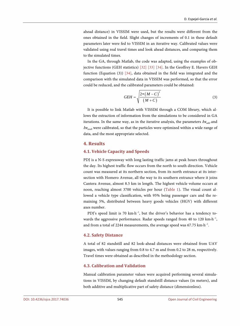
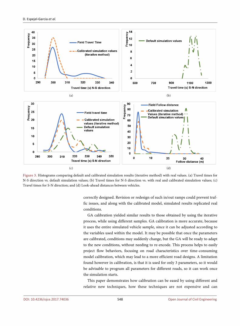
To validate calibration, a comparison between real, default and calibrated val-ues of travel times and follow distances was performed (Figure 3 and Figure 4). Data analysis of travel times and follow distances’ peaks show a similar behavior, thus validating the simulation. Histograms also reflect how simulated results us-ing adjusted VISSIM parameter values (presented in Table 2) match field data. Iterative (manual method) results do not precisely overlap with real and cali-brated travel time values (Figure 3(a)), however major peaks coincide, again va-lidating calibration; default values cannot be used in PDJ because they do not overlap and are offset (Figure 3(b), Figure 3(c)). Manual calibration offers then better results in follow distances (Figure 3(d)), with a major coincidence be-tween the major peaks.

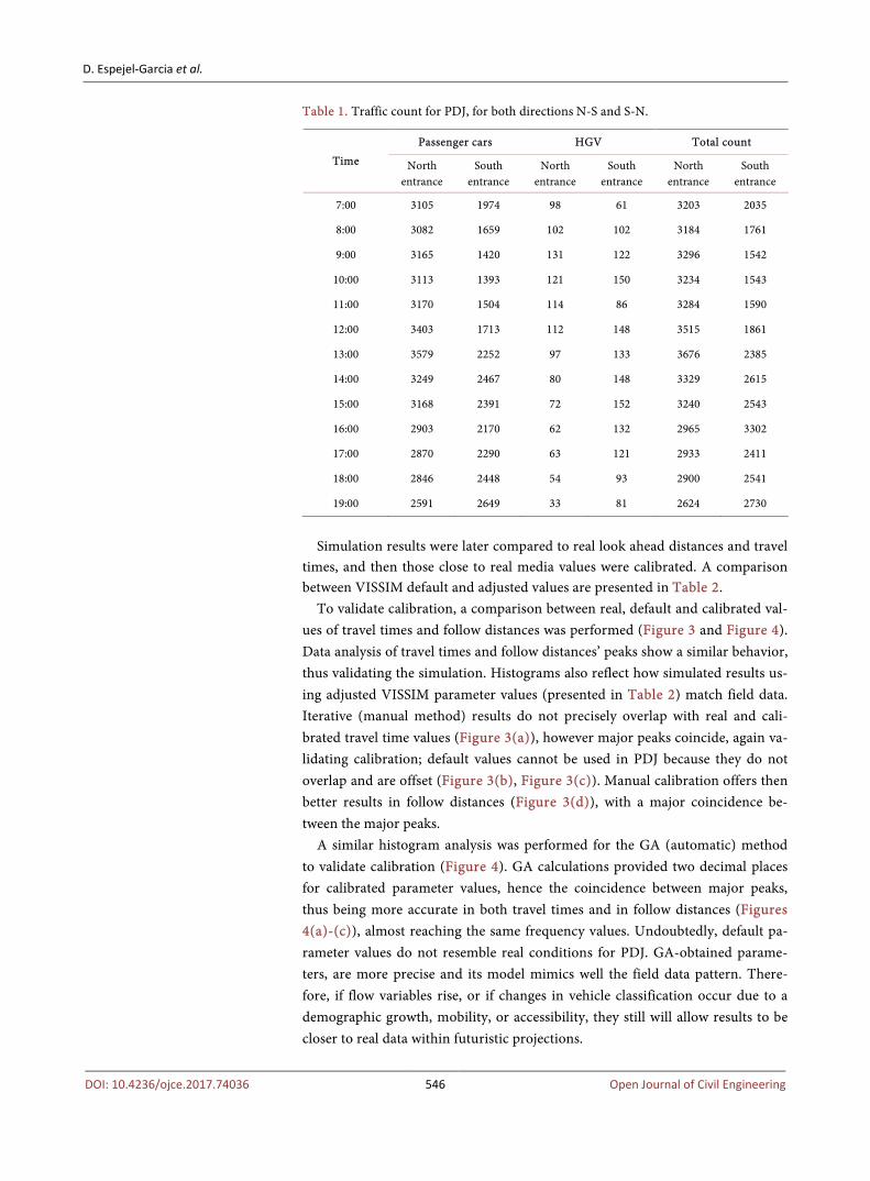
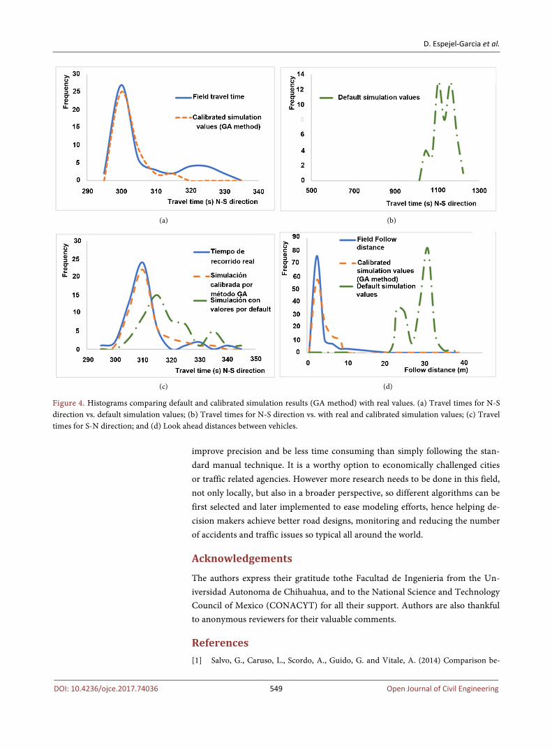
A similar histogram analysis was performed for the GA (automatic) method to validate calibration (Figure 4). GA calculations provided two decimal places for calibrated parameter values, hence the coincidence between major peaks, thus being more accurate in both travel times and in follow distances (Figures 4(a)-(c)), almost reaching the same frequency values. Undoubtedly, default pa-rameter values do not resemble real conditions for PDJ. GA-obtained parame-ters, are more precise and its model mimics well the field data pattern. There-fore, if flow variables rise, or if changes in vehicle classification occur due to a demographic growth, mobility, or accessibility, they still will allow results to be closer to real data within futuristic projections.

D. Espejel-Garcia et al.

DOI: 10.4236/ojce.2017.74036 547 Open Journal of Civil Engineering

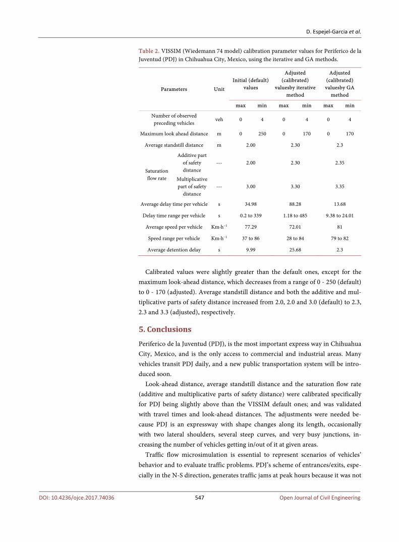
Table 2. VISSIM (Wiedemann 74 model) calibration parameter values for Periferico de la Juventud (PDJ) in Chihuahua City, Mexico, using the iterative and GA methods.

Parameters Unit

Initial (default) values

Adjusted (calibrated)

valuesby iterative method

Adjusted (calibrated) valuesby GA

method

max min max min max min

Number of observed preceding vehicles

veh 0 4 0 4 0 4

Maximum look ahead distance m 0 250 0 170 0 170

Average standstill distance m 2.00 2.30 2.3

Saturation flow rate

Additive part of safety distance

--- 2.00 2.30 2.35

Multiplicative part of safety

distance --- 3.00 3.30 3.35

Average delay time per vehicle s 34.98 88.28 13.68

Delay time range per vehicle s 0.2 to 339 1.18 to 485 9.38 to 24.01

Average speed per vehicle Km∙h−1 77.29 72.01 81

Speed range per vehicle Km∙h−1 37 to 86 28 to 84 79 to 82

Average detention delay s 9.99 25.68 2.3

Calibrated values were slightly greater than the default ones, except for the

maximum look-ahead distance, which decreases from a range of 0 - 250 (default) to 0 - 170 (adjusted). Average standstill distance and both the additive and mul-tiplicative parts of safety distance increased from 2.0, 2.0 and 3.0 (default) to 2.3, 2.3 and 3.3 (adjusted), respectively.

5. Conclusions

Periferico de la Juventud (PDJ), is the most important express way in Chihuahua City, Mexico, and is the only access to commercial and industrial areas. Many vehicles transit PDJ daily, and a new public transportation system will be intro-duced soon.

Look-ahead distance, average standstill distance and the saturation flow rate (additive and multiplicative parts of safety distance) were calibrated specifically for PDJ being slightly above than the VISSIM default ones; and was validated with travel times and look-ahead distances. The adjustments were needed be-cause PDJ is an expressway with shape changes along its length, occasionally with two lateral shoulders, several steep curves, and very busy junctions, in-creasing the number of vehicles getting in/out of it at given areas.

Traffic flow microsimulation is essential to represent scenarios of vehicles’ behavior and to evaluate traffic problems. PDJ’s scheme of entrances/exits, espe-cially in the N-S direction, generates traffic jams at peak hours because it was not

D. Espejel-Garcia et al.

DOI: 10.4236/ojce.2017.74036 548 Open Journal of Civil Engineering

(a) (b)

(c) (d)

Figure 3. Histograms comparing default and calibrated simulation results (iterative method) with real values. (a) Travel times for N-S direction vs. default simulation values; (b) Travel times for N-S direction vs. with real and calibrated simulation values; (c) Travel times for S-N direction; and (d) Look-ahead distances between vehicles.

correctly designed. Revision or redesign of such in/out ramps could prevent traf-fic issues, and along with the calibrated model, simulated results replicated real conditions.

GA calibration yielded similar results to those obtained by using the iterative process, while using different samples. GA calibration is more accurate, because it uses the entire simulated vehicle sample, since it can be adjusted according to the variables used within the model. It may be possible that once the parameters are calibrated, conditions may suddenly change, but the GA will be ready to adapt to the new conditions, without needing to re-encode. This process helps to easily project flow behaviors, focusing on road characteristics over time-consuming model calibration, which may lead to a more efficient road designs. A limitation found however in calibration, is that it is used for only 3 parameters, so it would be advisable to program all parameters for different roads, so it can work once the simulation starts.

This paper demonstrates how calibration can be eased by using different and relative new techniques, how these techniques are not expensive and can

D. Espejel-Garcia et al.

DOI: 10.4236/ojce.2017.74036 549 Open Journal of Civil Engineering

(a) (b)

(c) (d)

Figure 4. Histograms comparing default and calibrated simulation results (GA method) with real values. (a) Travel times for N-S direction vs. default simulation values; (b) Travel times for N-S direction vs. with real and calibrated simulation values; (c) Travel times for S-N direction; and (d) Look ahead distances between vehicles.

improve precision and be less time consuming than simply following the stan-dard manual technique. It is a worthy option to economically challenged cities or traffic related agencies. However more research needs to be done in this field, not only locally, but also in a broader perspective, so different algorithms can be first selected and later implemented to ease modeling efforts, hence helping de-cision makers achieve better road designs, monitoring and reducing the number of accidents and traffic issues so typical all around the world.

Acknowledgements

The authors express their gratitude tothe Facultad de Ingenieria from the Un-iversidad Autonoma de Chihuahua, and to the National Science and Technology Council of Mexico (CONACYT) for all their support. Authors are also thankful to anonymous reviewers for their valuable comments.

References [1] Salvo, G., Caruso, L., Scordo, A., Guido, G. and Vitale, A. (2014) Comparison be-

D. Espejel-Garcia et al.

DOI: 10.4236/ojce.2017.74036 550 Open Journal of Civil Engineering

tween Vehicle Speed Profiles Acquired by Differential GPS and UAV. 17th Meeting of the Euro Working Group on Transportation Ewgt 2014, Sevilla, 2-4 July 2014.

[2] Choa, F., Milam, R.T. and Stanek, D. (2003) CORSIM, PARAMICS and VISSIM: What the Manuals Never Told You. In: Benner, G. and Donnelly, R., Eds., Pro-ceedings of the Ninth TRB Conference on the Application of Transportation Plan-ning Methods, Baton Rouge, 6-10 April 2003, 392-402.

[3] Lownes, N.E. and Machemehl, R.B. (2006) VISSIM, a Multi-Parameter Sensitivity Analysis. In: Perrone, L.F., Wieland, F.P., Liu, J., Lawson B.G., Nicol, D.M. and Fu-jimoto, R.M., Eds., Proceedings of the 2006 Winter Simulation Conference IEEE Xplore, Monterrey, 3-6 December 2006, 1406-1413. https://doi.org/10.1109/WSC.2006.323241

[4] Fellendorf, M. and Vortisch, P. (2010) Microscopic Traffic Flow Simulator VISSIM. In: Barceló, J., Ed., Fundamentals of Traffic Simulation, International Series in Op-erations Research & Management Science, Springer, New York, 145, 63-93. https://doi.org/10.1007/978-1-4419-6142-6_2

[5] Wiedemann, R. (1974) Simulation des Straßenverkehrsflusses. (In German) Schtiftenreibe des Institus fur Verkehrswesen der Universitat Karlsruhe, Heft 8.

[6] Wiedemann, R. (1999) Modeling of RTI-Elements on Multi-Lane Roads. Advanced Telematics in Road Transport, Edited by the Comission of the European Community, DG XIII.

[7] Panwai, S. and Dia, H. (2005) Comparative Evaluation of Microscopic Car-Following Behavior. IEEE Transactions on Intelligent Transportation Systems, 6, 314-325. https://doi.org/10.1109/TITS.2005.853705

[8] Fedra, K. (2000) Urban Environmental Management: Monitoring GIS and Model-ing. Computers, Environment and Urban Systems, 23, 443-457. https://doi.org/10.1016/S0198-9715(99)00038-1

[9] Kim, S.J., Kim, W. and Rilett, L. (2005) Calibration of Microsimulation Models Us-ing Nonparametric Statistical Techniques. Transportation Research Broad of the National Academies, Washington DC, 111-119. https://doi.org/10.3141/1935-13

[10] Park, B. and Won, J. (2006) Microscopic Simulation Model Calibration and Valida-tion Handbook. Publication FHWA/VTRC 07-CR6. FHWA, U.S. Department of Transportation, Washington DC.

[11] Lee, D., Yang, X. and Chandrasekar, P. (2000) Parameter Calibration for PARAMICS Using Genetic Algorithm, Proceedings of 80th Annual Meeting of the Transportation Research Board, Washington, DC., 2000.

[12] Miller, D.M. (2009) Developing a Procedure to Identify Parameters for Calibration of a VISSIM Model. Master in Science Thesis, Georgia Institute of Technology, Georgia.

[13] Ma, T. and Abdulhai, B. (2002) Genetic Algorithm-Based Optimization Approach and Generic Tool for Calibrating Traffic Microscopic Simulation Parameters. Transportation Research Record: Journal of the Transportation Research Board, 1800, 6-15. https://doi.org/10.3141/1800-02

[14] Park, B. and Qi, H. (2005) Development and Evaluation of a Procedure for the Ca-libration of Simulation Models. Transportation Research Record: Journal of the Transportation Research Board, 1934, 208-217. https://doi.org/10.3141/1934-22

[15] Park, B. and Schneeberger, J. (2003) Microscopic Simulation Model Calibration and Validation: Case Study of VISSIM Simulation Model for a Coordinated Actuated Signal System. Transportation Research Record: Journal of the Transportation Re-

D. Espejel-Garcia et al.

DOI: 10.4236/ojce.2017.74036 551 Open Journal of Civil Engineering

search Board, 1856, 185-192. https://doi.org/10.3141/1856-20

[16] Rrecaj, A.A. and Bombol, K.M. (2015) Calibration and Validation of the VISSIM Parameters—State of the Art. TEM Journal-Technology Education Management Informatics, 4, 255-269.

[17] Censo de población y vivienda México (2010) INEGI (Instituto Nacional de Estadística y Geografía) http://www.inegi.org.mx/

[18] Carrasco, H. (2016) Supera Tráfico a Vialidades. El Diario de Juárez, June 2016. http://diario.mx/Local/2016-06-16_9d3948b1/supera-trafico-a-vialidades/

[19] Plan de Desarrollo Urbano del Centro de Población Chihuahua, Tercera Actualización. IMPLAN, H. Ayuntamiento de Chihuahua (2009). http://www.implanchihuahua.gob.mx/IMPLAN-Datos/PDU2040/pdf/PDU2040_2009/Documento/PDU2040_2009-02%20Diagnostico.pdf

[20] Quezada, M. and Barrientos, H. (2016) Se queda Chihuahua sin transporte público. El Diario de Chihuahua, July 2016. http://diario.mx/Estado/2016-07-02_1290468f/se-queda-chihuahua-sin-transporte-publico/

[21] Google Earth (2016) “Chihuahua City” 28°40’14.74” N and 106°05’24.63” W. Google Earth. October 6, 2017. November 22, 2017.

[22] US Department Transportation (2006) Traffic Detector Handbook. 3rd Edition, Vol. 1, FHWA-HRT-06-108, 1-2. http://www.fhwa.dot.gov/publications/research/operations/its/06108/06108.pdf

[23] Garber, N.J. and Hoel, L.A. (2005) Traffic and Highway Engineering. 5th Edition, Cengage Learning, Stamford.

[24] Leduc, G. (2008) Road Traffic Data: Collection Methods and Applications. Working Papers on Energy, Transport and Climate Change, 1(55).

[25] Cusack, B. and Khaleghparast, R. (2015). Evaluating Small Drone Surveillance Ca-pabilities to Enhance Traffic Conformance Intelligence. The Proceedings of the 8th Australian Security and Intelligence Conference, Perth, 30 November-2 December 2015, 21-27.

[26] VISSIM User’s Guide. PTV (Planung Transport Verkehr) VISSIM 8.0 (2014) http://www.et.byu.edu/~msaito/CE662MS/Labs/VISSIM_530_e.pdf

[27] Gardes, Y., May, A.D., Dahlgren, J. and Skabardonis, A. (2002) Freeway Calibration and Application of the PARAMICS Model. 81st Annual Meeting of the Transporta-tion Research Board, Washington DC.

[28] Chu, L., Liu, H.X., Oh, J.S. and Recker, W. (2003) A Calibration Procedure for Mi-croscopic Traffic Simulation. Intelligent Transportation Systems Proceedings, 2, 1574-1579.

[29] Moridpour, S., Sarvi, M., Rose, G. and Mazloumi, E. (2012) Lane-Changing Deci-sion Model for Heavy Vehicle Drivers. Journal of Intelligent Transportation Sys-tems, 16, 24-35. https://doi.org/10.1080/15472450.2012.639640

[30] Duong, D.D., Saccomanno, F.F. and Hellinga, B.R. (2011) Effects of Microscopic Traffic Platform Calibration on Errors in Safety and Traffic Metrics. 3rd Interna-tional Conference on Road Safety and Simulation, Indianapolis.

[31] Menneni, S., Sun, C. and Vortisch, P. (2008) Microsimulation Calibration Using Speed-Flow Relationships. Transportation Research Record: Journal of the Trans-portation Research Board, 2088, 1-9. https://doi.org/10.3141/2088-01

[32] Yang, Y., Dong, H., Qin, Y. and Zhang, Q. (2016) Parameter Calibration Method of

D. Espejel-Garcia et al.

DOI: 10.4236/ojce.2017.74036 552 Open Journal of Civil Engineering

Microscopic Traffic Flow Simulation Models Based on Orthogonal Genetic Algo-rithm. The 22nd International Conference on Distributed Multimedia Systems, Sa-lerno, 25-26 November 2016, 55-60.

[33] Manjunatha, P., Vortisch, P. and Mathew, T.V. (2013) Methodology for the Cali-bration of VISSIM in Mixed Traffic. Transportation Research Board 92nd Annual Meeting, 13-3677.

[34] UKHA (UK Highways Agency) (1975) Design Manual for Roads and Bridges. 12, Section 2.