A Comparison between Radiation Damage

Calculated with NASA-LaRCs HZETRN and with

GEANT4

A thesis submitted in partial fulfillment of the requirementfor the degree of Bachelor of Science

Physics from the College of William and Mary in Virginia,

by

Christopher E. Hendricks

Accepted for: BS in Physics

Advisor: W. J. Kossler

Gina Hoatson

Williamsburg, VirginiaMay 2007

Abstract

This project uses GEANT4, a Monte Carlo based program, to simulate radiation damage

caused by Galactic Cosmic Rays and Solar Particle Events. NASA uses a very different program,

the HZETRN, to simulate the passage of particles through shielding materials. The purpose of

this project is to determine the sources of discrepancies between the results of GEANT4 and

HZETRN seen in the thesis work of C. O’Neill.

i

Acknowledgements

I would like to thank Professor Kossler for all of his help throughout this project. In addition, C.

O’Neill’s previous work with GEANT4 formed the basis of this project. By contacting him, I was

able to become acquainted with the program and learn how it works.

ii

Contents

1 Introduction 1

2 Passage of Particles Through Shielding Materials 4

3 HZETRN and GEANT4 9

4 Progress to Date 12

5 Future Work 20

6 Conclusion 21

iii

1 Introduction

When discussing space radiation, there are three main sources of radiation to consider.

First are the inner and outer Van Allen belts which contain high energy electrons

trapped in the Earth’s geomagnetic field. While these protons have enough energy to

cause significant damage to astronauts and equipment, the time spent within these

belts is minimal. [1] For this reason, this source of radiation will be ignored for

the project. Instead, the project is focusing on the radiation damage caused by

both Galactic Cosmic Rays (GCR) and Solar Particle Events (SPE) and looking at

the effect of changing the thickness of shielding materials on the resulting radiation

damage experienced by astronauts.

Galactic cosmic rays are atomic nuclei that travel close to the speed of light.

The majority of GCRs have energies between the values of 100 MeV and 10 GeV.

These energies are equivalent to a proton traveling between 43 % to 99.6 % of the

speed of light. [2] However, the number of cosmic rays at these higher energies falls

off drastically after 1 GeV. [2] GCR spectrum consist mostly of protons and alpha

particles, however it also contains heavier particles including carbon, oxygen, silicon,

and iron.[3] These high charge and energy (HZE) ions cause a large amount of the

damage due to fragmentation when traveling through a shielding material.[1] The

fragmentation occurs when an incoming ion collides with a nucleus in the shielding

material with enough energy that both of the nuclei can shatter and form two or more

smaller nuclei. [4]

Solar Particle Events or Solar Energetic Particles, on the other hand, are created

when solar storms cause ions to accelerate to dangerously high energies such that they

can penetrate space suits and space ships.[1] These events can last up to a week and

the particles are mostly protons. While the protons of SPE are lighter, their higher

flux poses a significant risk.

GCRs are a constant source of radiation, however, SPEs are unpredictable and

1

could occur at any time. The Earths magnetic field offers protection from GCR

and SPE radiation on the Earth itself, however the concern is with long-term space

missions outside of this protection. Radiation damage has always been a concern

in space travel, however, as astronauts spend longer periods of time in space, it is

even more important to properly shield them from the hazards of radiation. It is

interesting to note that heightened solar activity can actually reduce the effects of

GCR radiation.[5] This is a result of magnetic fields being carried away from the

solar surface. Since it has been shown by several simulations that the relatively thin

shielding available for spacecraft cannot affect GCR dose, but can decrease SPE dose,

the lowest amount of radiation will be experienced inside a shielded environment

during one of these solar storms. This seems counterintuitive, but as long as the

astronaut is not caught outside of the spacecraft during one of these infrequent storms,

he or she is better off than in the absence of solar storms.

The effects of radiation can be both short and long-term and both are a concern

to NASA. The dose of radiation received in Grays is the energy in Joules deposited

in a kg of material. Another measure of the relative biological effectiveness (RBE) of

radiation is the sievert (Sv). This is obtained by multiplying the dose by an experi-

mentally determined quality factor and is known as Dose Equivalent.[1] This means

that the dose equivalent is very similar to dose, however it is simply multiplied by a

quality factor. Acute radiation sickness can occur with a radiation dose equivalent

greater than 1 Sv througout the course of a day. The ordinary amount of radiation

that Americans are exposed to over the course of a year is roughly 300 millirem. [6]

This is equivalent to 3 mSv over the course of a year. Receiving over 300 times this

yearly radiation dose induces radiation sickness.

In addition, the probability of vomiting and death increases as the radiation dose

increases. This radiation sickness is obviously a concern because it could delay or

compromise missions. An even more long term effect is the possibility of cancer

2

developing due to the radiation. NASA has set a 3 % risk of induced cancer guideline

and is even thinking about lowering this guideline to a lower value[1]. This means that

if the lifetime risk for cancer is around 20 %, NASA wants to prevent the lifetime risk

of cancer from increasing by 3 % and thus increasing the lifetime risk to 20.6 %. [7]

The more reliable information that can be gathered about the shielding of radiation,

the more NASA can be confident in sending astronuats on longer missions without

sacrificing safety guidelines.

0.01 1 100 10000E/Nucleon(MeV/u)

1e-06

0.0001

0.01

1

100

Flu

x (

Par

ticl

es/c

m^2*day

*M

eV)

p

HeCOSiFe

NASA GCR Spectrum

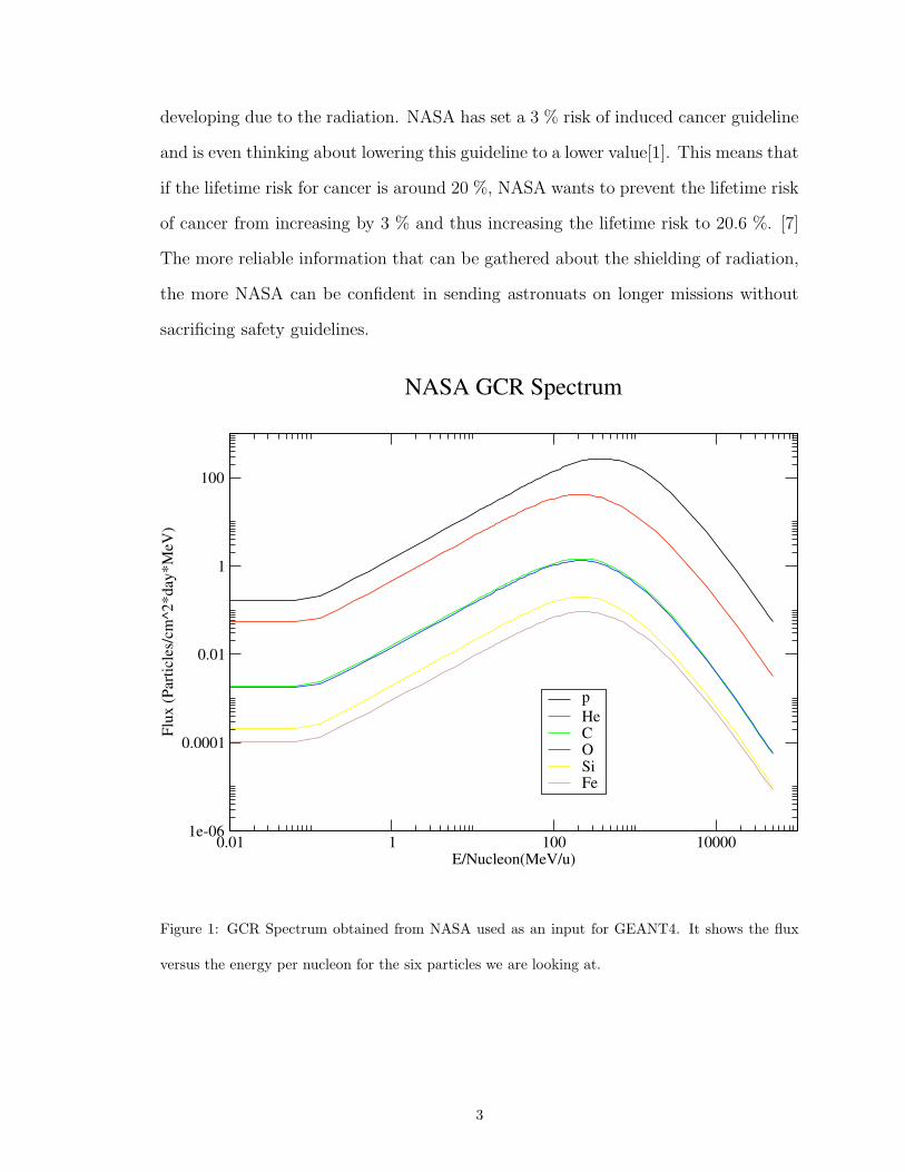
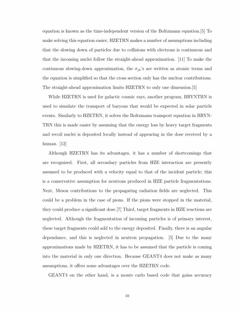
Figure 1: GCR Spectrum obtained from NASA used as an input for GEANT4. It shows the flux

versus the energy per nucleon for the six particles we are looking at.

3

1 10 100 1000 10000 1e+05Energy/Nucleon (MeV/u)

1e-05

0.0001

0.001

0.01

0.1

1

10

100

1000

10000R

elat

ive

Flu

ence

ProtonHeliumCarbonOxygen

SiliconIron

GEANT4 GCR Spectrum: Relative Fluence vs. Energy

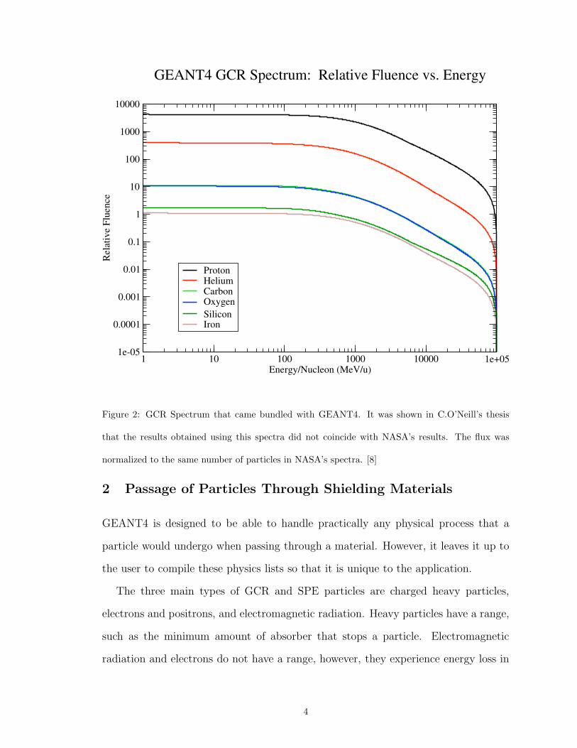
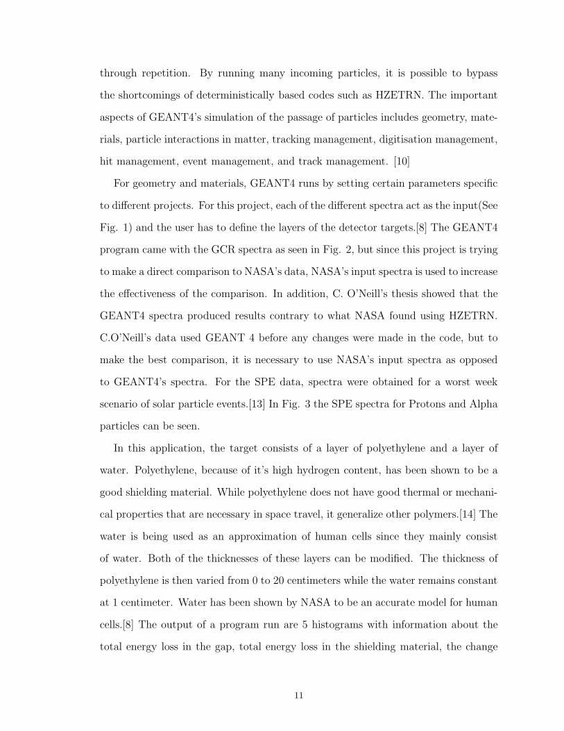
Figure 2: GCR Spectrum that came bundled with GEANT4. It was shown in C.O’Neill’s thesis

that the results obtained using this spectra did not coincide with NASA’s results. The flux was

normalized to the same number of particles in NASA’s spectra. [8]

2 Passage of Particles Through Shielding Materials

GEANT4 is designed to be able to handle practically any physical process that a

particle would undergo when passing through a material. However, it leaves it up to

the user to compile these physics lists so that it is unique to the application.

The three main types of GCR and SPE particles are charged heavy particles,

electrons and positrons, and electromagnetic radiation. Heavy particles have a range,

such as the minimum amount of absorber that stops a particle. Electromagnetic

radiation and electrons do not have a range, however, they experience energy loss in

4

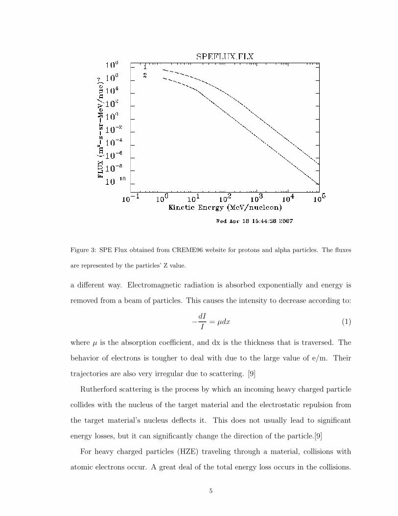
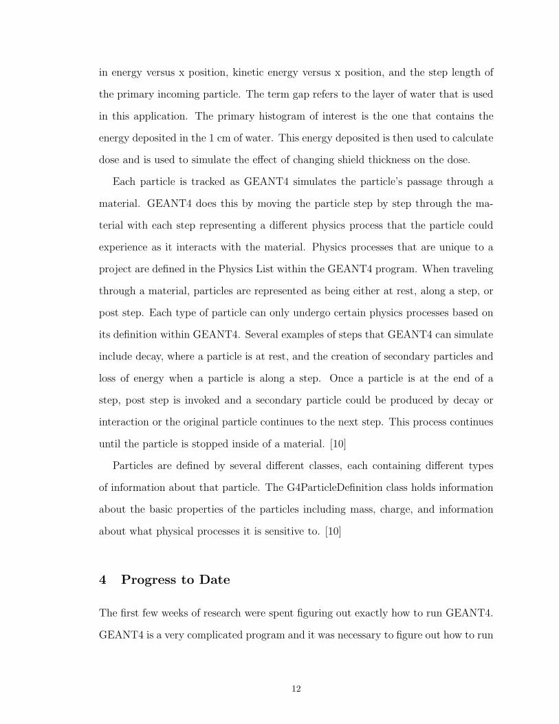
Figure 3: SPE Flux obtained from CREME96 website for protons and alpha particles. The fluxes

are represented by the particles’ Z value.

a different way. Electromagnetic radiation is absorbed exponentially and energy is

removed from a beam of particles. This causes the intensity to decrease according to:

−dI

I= µdx (1)

where µ is the absorption coefficient, and dx is the thickness that is traversed. The

behavior of electrons is tougher to deal with due to the large value of e/m. Their

trajectories are also very irregular due to scattering. [9]

Rutherford scattering is the process by which an incoming heavy charged particle

collides with the nucleus of the target material and the electrostatic repulsion from

the target material’s nucleus deflects it. This does not usually lead to significant

energy losses, but it can significantly change the direction of the particle.[9]

For heavy charged particles (HZE) traveling through a material, collisions with

atomic electrons occur. A great deal of the total energy loss occurs in the collisions.

5

Sometimes the atomic electrons are imparted with enough energy to escape their orbit

and move freely in the material.[9] As an example, consider a particle with charge

ze as it travels through a medium with N electrons/cm3. It is assumed that the

electrons are free and at rest and that the collision lasts for a short time so that the

electron receives the impulse without changing position during the collision. In this

case, the impulse is perpindicular to the trajectory of the incoming heavy particle

and is represented by the following equation:

∆p⊥ =∫

∞

−∞

e · E⊥dt =∫

e · E⊥

dx

v= z · e2

∫∞

−∞

1

r2· cos θ

dx

v(2)

where E⊥ is the perpindicular component of the electric field at position of the elec-

tron. The v is the velocity of the heavy particle and is assumed to be constant

throughout the collision. If we solve the second integral using Gauss’s theorem, we

obtain:[9]

Φ =∫

E⊥ · 2πb · dx = 4πze (3)

and

∆p =2 · z · e2

b · v(4)

Because the energy transferred equals (∆p)2/2m, and there are 2πNbdb · dx elec-

trons per length dx that have a distance between b and b+ db, the heavy ion will lose

energy per path length dx equal to:

−dE

dx= 2πN

∫bdb

(∆p)2

2m= 4πN

z2e4

mv2

∫ bmax

bmin

db

b= 4πN

z2e4

mv2log

bmax

bmin

(5)

For heavier particles, the energy loss to electrons far outweighs the energy loss due

to collisions with other nuclei. While lighter particles hit a nuclei, and lose energy in

that process, heavier particles can keep going without losing much energy.

The issue of multiple scattering has to be dealt with as well when looking at the

passage of different particles through the shielding materials. While Rutherford scat-

tering dealt with a single instance of scattering, a separate process needs to be defined

6

for multiple scattering where there is a cumulative effect of several different smaller

nuclear deflections that change the direction of the incoming particle. However, it

is hard to tell whether the change in direction θ is a result of just single scattering

or multiple scattering. The way it is often dealt with is by defining a θ1 where a

particle that only scatters once is likely to have an angle as large as θ1. If this is

the case, any scattering deflections larger than θ1 are most likely single scattering

events and any deflections less than θ1 are the result of multiple scattering. This is a

simple explanation, but the process of figuring out whether a deflection is the result

of multiple scatterings or just one scattering event is much more complicated.[9]

When electromagnetic radiation interacts with matter, three different types of

effects are seen. First, the photoelectric effect or photoelectric absorption which is a

process that is simulated in GEANT4 and other programs. If an incoming particle

has enough energy, it can remove one of the electrons from an inner shell of an atom

in the target material. The amount of energy required depends on what shell the

electron is being removed from and is described by the equation:

E = R · h · c ·(Z − σ)2

n2(6)

Rhc is the value 13.605 eV, Z is the atomic number, n is the principal quantum

number of the different electronic orbits, and σ is the screening constant and depends

on the different shells. Next, Thomson and Compton scattering can occur when

incoming photons scatter off of free electrons as opposed to the bound electrons that

cause the photoelectric effect. Thomson scattering is the same as Compton scattering,

but for low energies. Compton scattering is the process by which there is a change

of wavelength or frequency upon scattering and this theory can handle the particles

with higher energies. Third, Pair production is another phenomena that GEANT4

can simulate. It is also referred to as materialization and it takes place when a gamma

ray is transformed into an electron-positron pair. Since energy has to be conserved,

this cannot happen in free space, however, it can occur in the presence of a nucleus

7

or electron. It is possible for the electrons and positrons to gain significant momenta

from this pair production mechanism. Pairs can also be produced by heavy particle

collisions, electron-electron collisions, and the decay of mesons. [9]

For electrons travelling through a material at high speeds, the main source of

energy loss is the electromagnetic radiation that it emits due to acceleration. If the

energy of an electron is really low (E ≪ mc2), the loss of energy to radiation is very

small compared to ionization losses. The ratio of these losses is represented as:

(dE/dx)rad

(dE/dx)ion

=EZ

1600mc2=

EZ

800(7)

where E is in MeV. This equation shows that when the value EZ is large, the elec-

tromagnetic radiation dominates the ionization factor and when EZ is small, the

ionization loss is the predominate one. [9]

GEANT4 also deals with many different forms of decay through the G4Decay

class which implements both at rest and post-step actions for decaying particles.

there are already default tables for more common particles including π, K mesons,

Σ, Λ hyperons, and resonant baryons, but the user can also add more modifications.

GEANT4 figures out how a particle decays by using different decay models based on

the particle. For example, the V-A theory is used for muon decay. [10]

Finally, neutrons produced as secondary particles have to be accounted for in the

GEANT code. As opposed to charged particles or gamma rays which lose their en-

ergy through electromagnetic effects, neutrons primarily lose energy through nuclear

collisions. There are two types of collisions that can occur. The first type is an

inelastic collision where the nucleus gets excited by the neutron; the neutron must

have at least 1 MeV of energy for this to occur. If it doesn’t have this energy, the

neutron can only have elastic collisions. To figure out the loss of energy of neutrons

in these collisions, a center-of-mass system has to be described. If the nucleus that

the neutron strikes has a mass of A and the neutron has a velocity of V1, this makes

8

the velocity of the center of mass system, v1 equal to:

v1 = (A/(A + 1)) · V1 (8)

and the velocity of the target:

v2 = (−1/(A + 1)) · V1 (9)

The neutron velocity is the vector difference between these two velocities and the law

of cosines produces:

V ′2

1 = (AV1

A + 1)2 + (

V1

A + 1)2

− 2V 2

1 A(1

A + 1)2 =

V 21

(A + 1)2(A2 + 1 + 2A cos θ) (10)

where V ′

1 is the velocity of the neutron and θ is the scattering angle in the center-of-

mass system.

A lot of the information in this section came from Segre’s book Nuclei and Par-

ticles and an even more in depth description of these interactions can be gained by

consulting that text. [9]

3 HZETRN and GEANT4

HZETRN is a deterministic code that uses a one-dimensional space-marching formu-

lation of the Boltzmann transport equation. The Boltzmann transport equation takes

the form of:

Ω ·∇Φj(x, Ω, E) =∑k

∫σjk(Ω, Ω′, E, E ′) · Φk(x, Ω′, E ′)dE ′dΩ

′− σj(E) · Φj(x, Ω, E)

(11)

In this equation, σj is the total reaction cross section and the σjk values are the

channel changing cross sections. The Ω terms are vectors pointing in the direction of

the particles. HZETRN solves this Boltzmann equation for the particle flux, defined

as Φj(x, E) where j is the type of the ion with energy E and depth x. This particular

9

equation is known as the time-independent version of the Boltzmann equation.[5] To

make solving this equation easier, HZETRN makes a number of assumptions including

that the slowing down of particles due to collisions with electrons is continuous and

that the incoming nuclei follow the straight-ahead approximation. [11] To make the

continuous slowing-down approximation, the σjk’s are written as atomic terms and

the equation is simplified so that the cross section only has the nuclear contributions.

The straight-ahead approximation limits HZETRN to only one dimension.[5]

While HZETRN is used for galactic cosmic rays, another program, BRYNTRN is

used to simulate the transport of baryons that would be expected in solar particle

events. Similarly to HZETRN, it solves the Boltzmann transport equation in BRYN-

TRN this is made easier by assuming that the energy loss by heavy target fragments

and recoil nuclei is deposited locally instead of appearing in the dose received by a

human. [12]

Although HZETRN has its advantages, it has a number of shortcomings that

are recognized. First, all secondary particles from HZE interaction are presently

assumed to be produced with a velocity equal to that of the incident particle; this

is a conservative assumption for neutrons produced in HZE particle fragmentations.

Next, Meson contributions to the propagating radiation fields are neglected. This

could be a problem in the case of pions. If the pions were stopped in the material,

they could produce a significant dose.[7] Third, target fragments in HZE reactions are

neglected. Although the fragmentation of incoming particles is of primary interest,

these target fragments could add to the energy deposited. Finally, there is an angular

dependance, and this is neglected in neutron propagation. [5] Due to the many

approximations made by HZETRN, it has to be assumed that the particle is coming

into the material in only one direction. Because GEANT4 does not make as many

assumptions, it offers some advantages over the HZETRN code.

GEANT4 on the other hand, is a monte carlo based code that gains accuracy

10

through repetition. By running many incoming particles, it is possible to bypass

the shortcomings of deterministically based codes such as HZETRN. The important

aspects of GEANT4’s simulation of the passage of particles includes geometry, mate-

rials, particle interactions in matter, tracking management, digitisation management,

hit management, event management, and track management. [10]

For geometry and materials, GEANT4 runs by setting certain parameters specific

to different projects. For this project, each of the different spectra act as the input(See

Fig. 1) and the user has to define the layers of the detector targets.[8] The GEANT4

program came with the GCR spectra as seen in Fig. 2, but since this project is trying

to make a direct comparison to NASA’s data, NASA’s input spectra is used to increase

the effectiveness of the comparison. In addition, C. O’Neill’s thesis showed that the

GEANT4 spectra produced results contrary to what NASA found using HZETRN.

C.O’Neill’s data used GEANT 4 before any changes were made in the code, but to

make the best comparison, it is necessary to use NASA’s input spectra as opposed

to GEANT4’s spectra. For the SPE data, spectra were obtained for a worst week

scenario of solar particle events.[13] In Fig. 3 the SPE spectra for Protons and Alpha

particles can be seen.

In this application, the target consists of a layer of polyethylene and a layer of

water. Polyethylene, because of it’s high hydrogen content, has been shown to be a

good shielding material. While polyethylene does not have good thermal or mechani-

cal properties that are necessary in space travel, it generalize other polymers.[14] The

water is being used as an approximation of human cells since they mainly consist

of water. Both of the thicknesses of these layers can be modified. The thickness of

polyethylene is then varied from 0 to 20 centimeters while the water remains constant

at 1 centimeter. Water has been shown by NASA to be an accurate model for human

cells.[8] The output of a program run are 5 histograms with information about the

total energy loss in the gap, total energy loss in the shielding material, the change

11

in energy versus x position, kinetic energy versus x position, and the step length of

the primary incoming particle. The term gap refers to the layer of water that is used

in this application. The primary histogram of interest is the one that contains the

energy deposited in the 1 cm of water. This energy deposited is then used to calculate

dose and is used to simulate the effect of changing shield thickness on the dose.

Each particle is tracked as GEANT4 simulates the particle’s passage through a

material. GEANT4 does this by moving the particle step by step through the ma-

terial with each step representing a different physics process that the particle could

experience as it interacts with the material. Physics processes that are unique to a

project are defined in the Physics List within the GEANT4 program. When traveling

through a material, particles are represented as being either at rest, along a step, or

post step. Each type of particle can only undergo certain physics processes based on

its definition within GEANT4. Several examples of steps that GEANT4 can simulate

include decay, where a particle is at rest, and the creation of secondary particles and

loss of energy when a particle is along a step. Once a particle is at the end of a

step, post step is invoked and a secondary particle could be produced by decay or

interaction or the original particle continues to the next step. This process continues

until the particle is stopped inside of a material. [10]

Particles are defined by several different classes, each containing different types

of information about that particle. The G4ParticleDefinition class holds information

about the basic properties of the particles including mass, charge, and information

about what physical processes it is sensitive to. [10]

4 Progress to Date

The first few weeks of research were spent figuring out exactly how to run GEANT4.

GEANT4 is a very complicated program and it was necessary to figure out how to run

12

everything again. Because this project is a continuation of C. ONeills work, it was

difficult figuring out exactly what all of the files represented and how to import all of

the spectra into GEANT4. One of GEANT4’s main drawbacks is the amount of work

it takes to get acquainted with all of the nuances of the program. Once everything

was sorted out, it was possible to start running the spectra through the program.

It was possible to run the program with GCR spectra obtained from NASA. C.

O’Neill’s research used the GCR spectra that came with GEANT4 and he ran into

problems when comparing the data to NASA’s data. While NASAs radiation dose

was pretty much constant with changing shielding material depth, C. ONeills results

decreased dramatically before leveling out. This project resumes where C. O’Neill’s

ended. Unfortunately, even when using the GCR spectrum that NASA provided as

the input, the results still did not agree with the HZETRN results from NASA. At

this point, it seemed likely that something had to be wrong with the GEANT4 code

because both NASAs results and results using other Monte Carlo based codes[15]

showed that GCR radiation dose did not increase or decrease when the shielding

thickness was increased.

It was discovered that the main problem with the results was a consequence of

the way the Monte Carlo code was integrating the spectra. The Monte Carlo based

code is a process used to simulate data and this project is considering the process

by which an initial energy is chosen for a given particle. The NASA GCR spectra

serves as the probability distribution of GCR energies. For a particular particle such

that dP/dE(E)dE is the probablity of an energy between E and E + dE, one then

integrates this and normalizes, obtaining:

IP (E) =

E∫0

dP/dE ′dE ′

∞∫0

dP/dE ′dE ′

(12)

Then one uses a numeric random number generator to choose a number, r, between

13

0 and 1[7] and an energy, Es is chosen as indicated in Fig. 4

Figure 4: Monte Carlo selection of Energy

Originally, the code assumed that the spectra consisted of evenly spaced points.

However, the NASA GCR spectra used to run the program had a lot of data clustered

around the lower energies and data that was more spread out as the energy was

increased. This discrepancy turned out to have a huge effect on the results. To correct

this mistake, the code was modified to take the difference between one energy and

the next energy and then multiplied this difference by the average of the probability

of energy to get an approximate integral of the spectra.

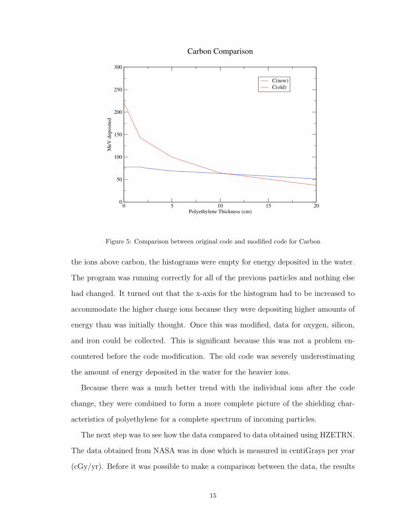
The difference between the results from the original code and results from the

modified code is obvious in Fig. 5. The energy does not change nearly as much with

changing shielding thicknesses as it did before the code was changed and it should

be at least a little bit closer to NASAs results once all of the incoming particles are

combined together. However, there is still a decrease in the energy deposited as the

shielding thickness is increased. This trend is also seen in all of the other ions which

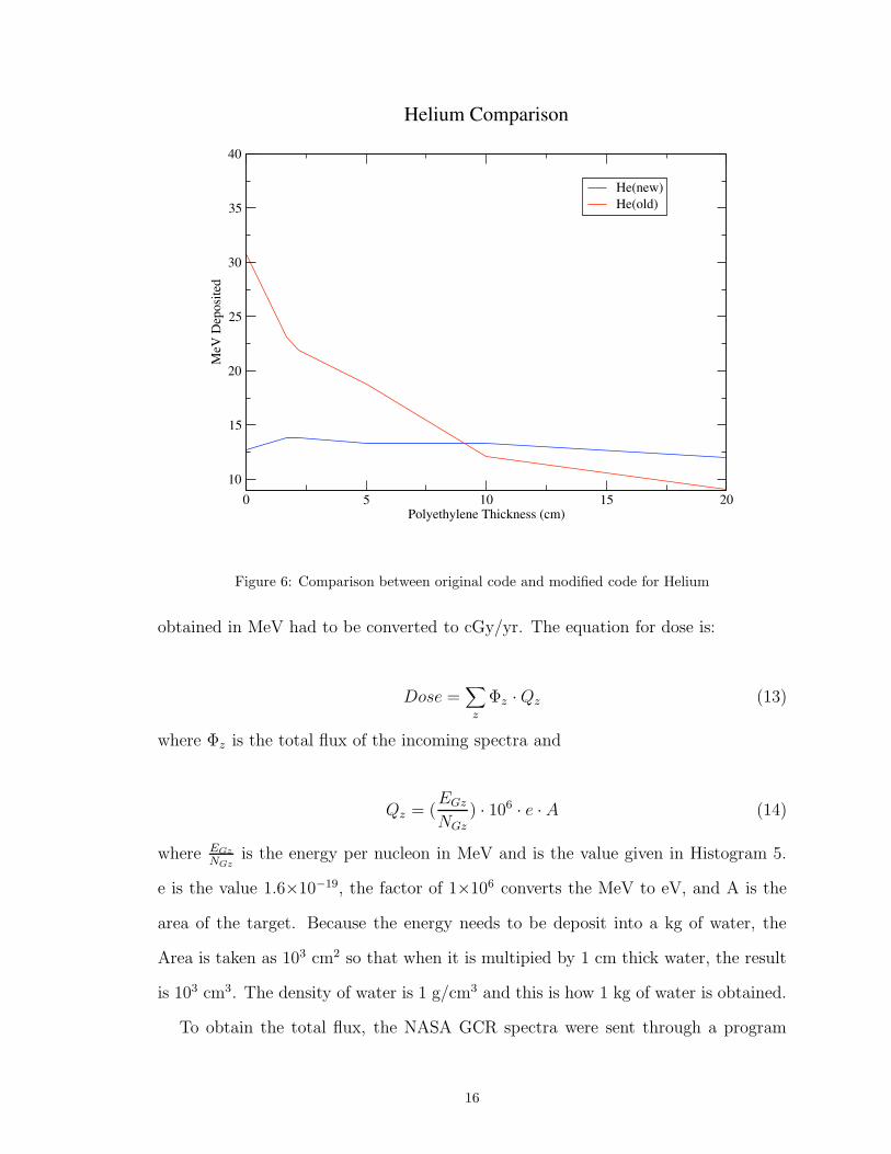
is promising. The modified code allowed for much less change in dose with changing

shield thickness as seen in Fig.6.

One final problem encountered was found after modifying the code. For any of

14

0 5 10 15 20Polyethylene Thickness (cm)

0

50

100

150

200

250

300

MeV

dep

osi

ted

C(new)

C(old)

Carbon Comparison

Figure 5: Comparison between original code and modified code for Carbon

the ions above carbon, the histograms were empty for energy deposited in the water.

The program was running correctly for all of the previous particles and nothing else

had changed. It turned out that the x-axis for the histogram had to be increased to

accommodate the higher charge ions because they were depositing higher amounts of

energy than was initially thought. Once this was modified, data for oxygen, silicon,

and iron could be collected. This is significant because this was not a problem en-

countered before the code modification. The old code was severely underestimating

the amount of energy deposited in the water for the heavier ions.

Because there was a much better trend with the individual ions after the code

change, they were combined to form a more complete picture of the shielding char-

acteristics of polyethylene for a complete spectrum of incoming particles.

The next step was to see how the data compared to data obtained using HZETRN.

The data obtained from NASA was in dose which is measured in centiGrays per year

(cGy/yr). Before it was possible to make a comparison between the data, the results

15

0 5 10 15 20Polyethylene Thickness (cm)

10

15

20

25

30

35

40

MeV

Dep

osi

ted

He(new)

He(old)

Helium Comparison

Figure 6: Comparison between original code and modified code for Helium

obtained in MeV had to be converted to cGy/yr. The equation for dose is:

Dose =∑z

Φz · Qz (13)

where Φz is the total flux of the incoming spectra and

Qz = (EGz

NGz

) · 106· e · A (14)

where EGz

NGzis the energy per nucleon in MeV and is the value given in Histogram 5.

e is the value 1.6×10−19, the factor of 1×106 converts the MeV to eV, and A is the

area of the target. Because the energy needs to be deposit into a kg of water, the

Area is taken as 103 cm2 so that when it is multipied by 1 cm thick water, the result

is 103 cm3. The density of water is 1 g/cm3 and this is how 1 kg of water is obtained.

To obtain the total flux, the NASA GCR spectra were sent through a program

16

that was able to approximately integrate it according to the equation:

Φz =∑

i

(Ei) − (Ei+1) ·1

2· (Fi + Fi+1) (15)

where Ei is the energy value on the x-axis of the GCR Spectra (See Fig. 1) and Fi is

the value of the flux on the y-axis of the same graph.

The result of these equations is in the units of Grays per day, which is not exactly

the units necessary for comparison. The final step was to multiply by 3.65 × 104 to

convert it into cGy/yr to coincide with NASA’s units.

The dose of the different particles was obtained using these equations and after

adding all of the ions together for each thickness of polyethylene it was possible to

make a comparison to the NASA data [16]. The trends are very similar between the

two, but since they are not the same material, a direct comparison wasn’t possible.

The HZETRN data that was available for comparison with GEANT4 data made use

out of the Martian Regolith as the shielding material. Regolith is defined as a layer of

unconsolidated rocky material covering solid rock. NASA wanted to see how effective

shielding material made from Martian rocks and regolith was affected by radiation.

By adding an epoxy, and thus increasing the hydrogen content, NASA speculated

that the regolith could serve as a shielding material if structures were to be built on

the surface in the future. This is important because it makes sense to use materials

already present on Mars for building structures.[16] If there is more knowledge about

the shielding characteristics of martian regolith, a plan for its utilization as a building

material can be determined. The elemental constituents of the regolith were also

found in the article that contained the regolith data.[16] The regolith consists almost

entirely of five different elements and has a density of 1.4 g/cm3. The elements

and their percentage composition are as follows: Oxygen (62.5%), Silicon (21.77 %),

Iron (6.73 %), Magnesium (6.06%), and Calcium (2.92 %). [16] Using GEANT4’s

ExN03DetectorConstruction source file, a new Martian Regolith target was added as

the elements that were not already included in the code including Magnesium, Iron,

17

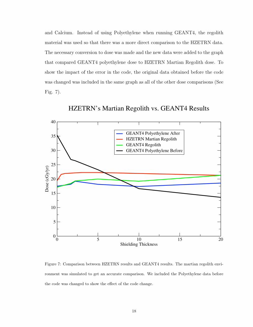
and Calcium. Instead of using Polyethylene when running GEANT4, the regolith

material was used so that there was a more direct comparison to the HZETRN data.

The necessary conversion to dose was made and the new data were added to the graph

that compared GEANT4 polyethylene dose to HZETRN Martian Regolith dose. To

show the impact of the error in the code, the original data obtained before the code

was changed was included in the same graph as all of the other dose comparisons (See

Fig. 7).

0 5 10 15 20Shielding Thickness

0

5

10

15

20

25

30

35

40

Do

se (

cGy

/yr)

GEANT4 Polyethylene After

HZETRN Martian Regolith

GEANT4 Regolith

GEANT4 Polyethylene Before

HZETRN’s Martian Regolith vs. GEANT4 Results

Figure 7: Comparison between HZETRN results and GEANT4 results. The martian regolith envi-

ronment was simulated to get an accurate comparison. We included the Polyethylene data before

the code was changed to show the effect of the code change.

18

As seen in Fig. 7, the change in code was necessary. It was later discovered that

Dr. Susan Guatelli, author of the CERN cosmic ray simulation examples code was

aware of this problem with the code and had updated it in the newest version. The

Polyethylene looks very similar to the Martian Regolith data obtained by NASA,

however it is shifted downward. The GEANT4 regolith data that were collected

shifted the curve up a bit more and improves confidence in the results.

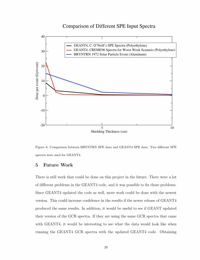
The SPE results were not as promising as the GCR results because the shapes of the

graphs were different. Using two different SPE spectra, it was not possible to replicate

results found using BRYNTRN. To make comparisons between the BRYNTRN data

and our data, we converted the energy deposited in the water from MeV to Gy/event

in a matter similar to that used for the GCR data. The only differences were that

the time interval considered was a week and the flux was converted from per radian

to per 2π radians.

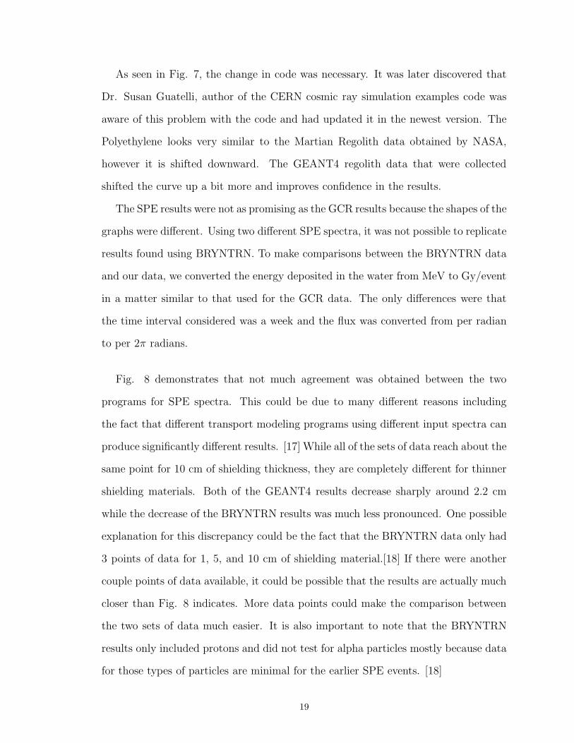
Fig. 8 demonstrates that not much agreement was obtained between the two

programs for SPE spectra. This could be due to many different reasons including

the fact that different transport modeling programs using different input spectra can

produce significantly different results. [17] While all of the sets of data reach about the

same point for 10 cm of shielding thickness, they are completely different for thinner

shielding materials. Both of the GEANT4 results decrease sharply around 2.2 cm

while the decrease of the BRYNTRN results was much less pronounced. One possible

explanation for this discrepancy could be the fact that the BRYNTRN data only had

3 points of data for 1, 5, and 10 cm of shielding material.[18] If there were another

couple points of data available, it could be possible that the results are actually much

closer than Fig. 8 indicates. More data points could make the comparison between

the two sets of data much easier. It is also important to note that the BRYNTRN

results only included protons and did not test for alpha particles mostly because data

for those types of particles are minimal for the earlier SPE events. [18]

19

5 10Shielding Thickness (cm)

-20

-10

0

10

20

30

40D

ose

per

ev

ent

(Gy

/ev

ent)

GEANT4, C. O’Neill’s SPE Spectra (Polyethylene)

GEANT4, CREME96 Spectra for Worst Week Scenario (Polyethylene)

BRYNTRN 1972 Solar Particle Event (Aluminum)

Comparison of Different SPE Input Spectra

Figure 8: Comparison between BRYNTRN SPE data and GEANT4 SPE data. Two different SPE

spectra were used for GEANT4.

5 Future Work

There is still work that could be done on this project in the future. There were a lot

of different problems in the GEANT4 code, and it was possible to fix those problems.

Since GEANT4 updated the code as well, more work could be done with the newest

version. This could increase confidence in the results if the newer release of GEANT4

produced the same results. In addition, it would be useful to see if GEANT updated

their version of the GCR spectra. If they are using the same GCR spectra that came

with GEANT4, it would be interesting to see what the data would look like when

running the GEANT4 GCR spectra with the updated GEANT4 code. Obtaining

20

data for other shielding materials could also prove useful to show the wide range of

shielding possibilities. In addition, code could be added to the program to add a new

histogram that gives the dose and the dose equivalent of the deposited radiation.

6 Conclusion

In his thesis, C. O’Neill used Polyethylene as a shielding material instead of martian

regolith. However, this should not account for the results that he saw because the only

discrepancy should be a shift of the graph. His main problem dealt with the shape of

the curve for GCR dose when compared to shielding thickness. This project sought

to more closely replicate results obtained by NASA using the HZETRN code. The

major obstacle of this project was the discovery of incorrect code within GEANT4.

Once the code modification was made and this error was corrected, it was possible

to make a more direct comparison to NASA’s results. The results using the newly

modified code and Polyethylene as a shielding material produced a similar shape to

NASA’s data. After creating a regolith shielding material in GEANT4, the results

were within 5 % of NASA’s results. GEANT4 also updated their code and this new

version included a fix to the error that was found when resolving the discrepancies

between results. Because this code change was discovered by the authors of GEANT,

there is much more of a reason to trust the data that the modified version of GEANT4

produced. For even more confidence in results, it would be useful to install the newest

version of GEANT4. Finally, HZETRN may be updated in the future to include

all 3 dimensions. This could actually prove very useful because it might actually

reduce some of the discrepancy seen between GEANT4 and HZETRN. HZETRN’s

main disadvantage is the fact that it can only operate in one dimension due to it’s

assumptions, so this could help increase confidence in all results. [19]

21

References

[1] Radiation and the International Space Station: Recommendations to Reduce Risk,

2000.

[2] R. A. Mewaldt. Cosmic Rays, 1996. www.srl.caltech.edu/personnel/dick/cos encyc.html.

[3] NASA’s Cosmicopia - Galactic Cosmic Rays, 2006. helios.gsfc.nasa.gov/gcr.html.

[4] P. Scampoli et al. Fragmentation studies of relativistic iron ions using plastic

nuclear track detectors. Advances in Space Research, 35:230, 2005.

[5] John W. Wilson. HZETRN: Description of a Free-Space Ion and Nucleon Trans-

port and Shielding Computer Program, 1995. Pages 3 - 32.

[6] Fact Sheet on Biological Effects of Radiation, 2007. www.nrc.gov/reading-

rm/doc-collections/fact-sheets/bio-effects-radiation.html.

[7] W. J. Kossler. Personal Communication, 2006.

[8] Christopher O’Neill. Computer Simulations of Radiation Shiedling Materials for

Use in the Space Radiation Environment, 2006.

[9] Emilio Segre. Nuclei and Particles, chapter 2. W. A. Benjamin, Inc., New York,

New York, 1964.

[10] S. Agostinelli et al. GEANT4 - a simulation toolkit, 2003. Pages 272 - 279.

[11] P. Saganti et al. Marie measurements and model predictions of solar modulation

of galactic cosmic rays. 29th International Cosmic Ray Conference Pune, 00:101–

104, 2005.

[12] J. W. Wilson et. al. Shielding Strategies for Human Space Exploration, 1997.

[13] United States Navy. Cosmic Ray Effects on Micro Electronics, 2007.

https://creme96.nrl.navy.mil/ This webpage allows users to create spectra based

on different criteria.

22

[14] Fire Away, Sun, and Stars! Shields to Protect Future Space Crews, 2004.

http://www.nasa.gov/vision/space/travelinginspace/radiation shielding.html.

[15] F. Ballarini et al. Gcr and spe organ doses in deep space with different shielding:

Monte carlo simulations based on the fluka code coupled to anthropomorphic

phantoms. Advances in Space Research, 37:1791, 2006.

[16] Myung-Hee Y. Kim et al. Comparison of Martian Meteorites and Martian Re-

golith as Shield Materials for Galactic Cosmic Rays, 1998. Pages 5-10.

[17] Lawrence W. Townsend et. al. Dose uncertainties for large solar particle events:

Input spectra variability and human geometry approximations. Radiation Mea-

surements, 30:337 – 343, 1998.

[18] Lawrence W. Townsend. Implications of the space radiation environment for

human exploration in deep space. Radiation Protection Dosimetry, 115:44–50,

2005.

[19] Lawrence W. Townsend. Nasa space radiation transport code development con-

sortium. Radiation Protection Dosimetry, 116:118–122, 2005.

23