A Comparison of Actuarial Financial Scenario Generators - Variance

A Comparison of Actuarial FinancialScenario Generators

by Kevin C. Ahlgrim, Stephen P. D’Arcy, and Richard W. Gorvett

ABSTRACT

Significant work on the modeling of asset returns and othereconomic and financial processes is occurring within theactuarial profession, in support of risk-based capital analy-sis, dynamic financial analysis, pricing embedded options,solvency testing, and other financial applications. Althoughthe results of most modeling efforts remain proprietary, twomodels are in the public domain. One is the CAS-SOA re-search project, Modeling of Economic Series Coordinatedwith Interest Rate Scenarios. The other was developed asthe result of American Academy of Actuaries study in sup-port of the C-3 Phase 2 RBC for Variable Annuities. Bothdata sets provide practitioners with a large number of iter-ations for key financial values, including short- and long-term interest rates and equity returns. This paper examinesthe role of stochastic modeling in actuarial work, focus-ing on a comparison of the underlying models and theiroutputs, to determine the impact of the use of differentassumptions and parameter selection on the modeling pro-cess.

KEYWORDS

Financial scenario generator, stochastic modeling, risk-based capital,interest rates, inflation, equity returns, cash flow testing

VOLUME 2/ISSUE 1 CASUALTY ACTUARIAL SOCIETY 111

Variance Advancing the Science of Risk

1. IntroductionIn May 2001, the Casualty Actuarial Society

(CAS) and the Society of Actuaries (SOA) jointlyissued a request for proposals on the researchtopic “Modeling of Economic Series Coordinatedwith Interest Rate Scenarios.” The objectives ofthis request were to develop a research relation-ship with persons selected to investigate thistopic; produce a literature review of work pre-viously done in the area of economic scenariomodeling; determine appropriate data sourcesand methodologies to enhance economic mod-eling efforts relevant to the actuarial profession;and produce a working model of economic se-ries, coordinated with interest rates, that couldbe made public via the CAS and SOA Web sitesand used by actuaries to project future economicscenarios. Categories of economic series to bemodeled included interest rates, equity price lev-els, inflation rates, unemployment rates, and realestate price levels. In addition to providing thefinancial scenario generator model, this projectalso produced a set of output scenarios for theseeconomic series that could be used directly infinancial analysis. This work is summarized inAhlgrim, D’Arcy, and Gorvett (2004b; 2005).The Life Capital Adequacy Subcommittee

(LCAS) of the American Academy of Actuar-ies (AAA) recommended in a series of reports(1999; 2002; 2005) that life insurers implementnew tests of capital adequacy which utilize sto-chastic models for scenario testing of variableproducts with guarantees. Although the ultimaterecommendation is for each insurer to develop itsown models, the LCAS encouraged the AAA toprovide 10,000 prepackaged scenarios that couldbe used as an alternative to internal models.As a result of these two projects, practitioners

now have a choice between two publicly avail-able financial scenario generators. This paper willserve to explain the underlying processes used ineach of the models, compare the output valuesfor common factors, and describe the issues

that should be considered when using thesemodels.The remainder of this paper is organized as

follows. Section 2 describes the historical devel-opment of actuarial modeling of economic andfinancial processes, highlighting the growth inpopularity of stochastic modeling. Section 3 pro-vides some background on risk-based capitalwhich has become one of the primary uses ofstochastic modeling. Section 4 discusses themathematical and economic details underlyingeach of the two publicly available financial sce-nario models. Section 5 analyzes and comparesthe output and results from each model. Section6 illustrates the impact of these differences usingtwo separate actuarial applications.

2. Stochastic modeling

Actuarial analysis has progressed through sev-eral stages of development regarding the useof economic variables. Initially, the standard ap-proach was to use deterministic values for in-terest rates, equity returns, and other key finan-cial variables. Judgment was used to estimate therange of expected outcomes and to value embed-ded options such as investment return and mini-mum benefit guarantees. This approach often ledto the mispricing of key features of insurancepolicies and consequent financial difficulties fora number of insurers. Many of these problemswere due to inadequately reflecting the potentialrisk and volatility associated with dynamic eco-nomic and financial conditions.Given the disappointing results of determin-

istic assumptions, actuaries began to recognizethe inherent uncertainty surrounding economicvariables through predetermined scenarios. Forexample, New York regulation 126 requires in-surers to test asset adequacy and assess theirresulting hypothetical financial conditions un-der seven prescribed interest rate scenarios. Al-though these prespecified scenarios marked animprovement over the deterministic approach, the

112 CASUALTY ACTUARIAL SOCIETY VOLUME 2/ISSUE 1

A Comparison of Actuarial Financial Scenario Generators

use of a limited number of scenarios provided noindication of the relative frequency of any par-ticular outcome, and typically did not reflect thefull range of economic conditions that could beexpected to occur.The latest stage in actuarial analysis has been

the development of stochastic models to reflectthe underlying uncertainty of economic and fi-nancial variables (Wilkie 1986; 1995; Hibbert,Mowbray, and Turnbull 2001). When these so-phisticated models are properly developed, theycan be used to more accurately price embeddedoptions in insurance contracts, to set appropri-ate solvency margins for diverse insurance op-erations, and to evaluate alternative operationalchoices within an insurer. Stochastic models formthe basis of dynamic financial analysis (DFA),in which the underwriting and investment com-ponents of an insurance company are evaluated,in aggregate, under a large number of potentialfuture environments. Stochastic models are alsoused in regulation to set risk-based capital (RBC)levels and by rating agencies to establish com-pany ratings.One of the major concerns raised by the

Morris Review of the Actuarial Profession in GreatBritain (2004) is that actuaries failed to adequate-ly reflect particular interest rate paths and eq-uity returns over the last decade. Recent advancesin the field of financial economics, combinedwith the increased power and speed of comput-ers, have provided actuaries with powerful sto-chastic modeling tools. However, understandingthe diverse models that have been proposed, andappreciating their underlying philosophical andtechnical differences, is a significant challenge.

3. Risk-based capital

One of the primary uses of stochastic mod-els is in establishing regulatory capital require-ments for insurers. The history of capital stan-dards in insurance shares a similar progressionto actuarial assumptions for financial variables.

Initial capital standards were simply flat amountsthat did not reflect relative risk levels. Minimummargin requirements for European insurers be-gan to be set based on the risks inherent in acompany. By the mid-1990s, regulation in theUnited States, Japan, and other countries movedto a RBC system to define the minimum level ofcapital an insurer must hold to avoid impositionof regulatory controls. The formula attempted tobetter correlate an insurer’s inherent risk withits required surplus position. To determine tar-get surplus amounts, RBC factors (or loads) areapplied to statutory statement data. Whereas themost dominant risks of life insurers are asset andinvestment risks, liability and pricing risks aremore crucial for property-liability insurers.

3.1. RBC risk types

Since risks have different consequences foreach type of insurer, separate RBC formulas havebeen developed. While the relative weights ofrisks may be different, the types of risks facedby insurers are identical. Some of these include:

² Asset or investment risks. Capital is requiredto offset the potential loss in market value ofthe insurer’s asset portfolio. Higher factors areused for classes of assets that inherently havemore risk. For example, the RBC factor ap-plied to stocks is significantly higher than in-vestment grade bonds.

² Insurance/underwriting risks. Given the in-evitable random fluctuations in an insurer’sloss experience, RBC is used to protect policy-holders from the inherent uncertainty in an in-surer’s liabilities. Since the risk characteristicsof each line of business are unique, differentcapital charges are separately applied to eachproduct. For life insurers, RBC charges are ap-plied to the net amount of risk over and aboveestablished reserves. For property-liabilitylines, the RBC charge is applied to existingloss reserves and written premium amounts.



² Business risks. These charges stem from var-ious risks that may not be covered by otherRBC charges, such as loan guarantees to sub-sidiaries and reinsurance default. While mea-suring these risks is difficult, the general ap-proach is based on the potential assessment bystate guaranty funds.

Life insurers also include a charge for asset-liability management (ALM) risk. In addition tothe capital charges levied to reflect the under-lying asset risk, an additional layer of risk ispresent if the values of insurer liabilities are notperfectly coordinated with asset movements. Tra-ditional asset/liability risk is based on the po-tential mismatch of interest rate sensitivities be-tween the invested assets of the insurer and theirpolicy obligations. For example, if an insurer at-tempts to obtain a higher interest rate by extend-ing the maturity of their bond portfolio (with nochange in the duration of liabilities), the insurerhas increased its interest rate exposure. Shouldyields increase, the value of assets will declinemore than the value of the liabilities and thesurplus position of the life insurer is impaired.Given the potential for interest rate risk mis-matches, the insurer is required to hold a largeramount of capital to support this risk. In thelife insurer RBC formula, these risks are termedC-3 risks. In contrast, the value of liabilities forproperty-liability insurers remains fairly stablewith respect to interest rate changes since statu-tory reserves are not discounted, although themarket value of the liabilities would be impactedby interest rate changes (see Ahlgrim, D’Arcy,and Gorvett 2004a and D’Arcy and Gorvett 2000for a fuller analysis of this issue).In the early development of the RBC formula,

C-3 risks were coined interest rate risks. Tra-ditional life insurance products are affected byinterest rates since the value of policy benefitsand policyholder options is closely related to in-terest rate movements. The potential mismatchbetween the cash flows of assets and liabilities

are most severe with products that have substan-tial favorable policyholder guarantees (embed-ded options), notably single premium life prod-ucts and annuities with rate guarantees. Recentlife insurance product development, especiallyvariable annuities and other equity indexed prod-ucts, pose additional challenges given the height-ened sensitivity of liability values to changesin stock market prices. Therefore, the nature ofC-3 risks now encompasses broader asset/liabil-ity matching risks, not just interest rate risk.

3.2. American Academy of ActuariesRBC guidance

Over time it became evident that the one-size-fits-all application of RBC factors to assessC-3 risk was insufficient to adequately differenti-ate weakly capitalized insurers from adequatelycapitalized ones. Given the development of alltypes of product variations issued by insurers, itwas recognized that a single factor which blan-kets all insurance products would not fit everysituation. At the request of the National Asso-ciation of Insurance Commissioners (NAIC), theLife Risk-Based Capital Task Force of the Amer-ican Academy of Actuaries began to investigatealternative approaches to better reflect C-3 riskof life insurers.In October 1999, the task force released its

“Phase I Report” (AAA 1999), which providesinitial guidance for life insurance companies tomeasure ALM risks. The report focuses on prod-ucts with substantial interest rate guarantees, pri-marily annuities and single premium life prod-ucts. These guidelines were implemented effec-tive December 31, 2000.Building upon the modeling techniques that

became widespread for asset adequacy testing,the task force recommended scenario testing as atool for establishing appropriate capital standardsinstead of the application of RBC factor load-ings. The Academy’s aim is to set capital require-ments based on the 95th percentile of the dis-



tribution stemming from interest rate risks. TheAcademy’s approach stresses modeling underreal-world probability measures. While the risk-neutral measure is important for pricing, it is notuseful when estimating the tails of the distribu-tion which ultimately determines the risk expo-sure for life insurers.To facilitate development of internal propri-

etary stochastic models, the Academy providesspecific guidance on generating interest rate sce-narios. In lieu of developing their own models,companies may choose to use prepackaged sce-narios, which are posted on the Academy’s Website. Details of their interest rate model are de-scribed in Section 4.The Phase I report acknowledges that C-3 risk

consists of more than just interest rate risk. Re-cent product innovation also incorporates signif-icant equity risk and has greatly expanded theasset/liability risks of insurers. In 2005, theAcademy’s task force (now under the name LifeCapital Adequacy Subcommittee or LCAS) ad-dressed the equity-related component of C-3 riskby releasing its “Phase II Report” (AAA 2005).These guidelines include “certain standards thatmust be satisfied” when developing equity re-turn scenarios. For example, Appendix 2 ofthe June 2005 report includes a “table of calibra-tion points” as a cumulative distribution func-tion of stock returns over various investmenthorizons.The LCAS report describes several reasonable

approaches to equity modeling. All of these ap-proaches are variations and extensions on theBlack-Scholes geometric Brownian motion as-sumption for stock price movements. While notlimiting actuaries to those included, the Acad-emy’s report specifically mentions three equitysimulation models:

² Independent lognormal (ILN), where (contin-uous) stock returns are normally distributed.However, the report highlights the fat-tailednature of historical stock returns over short

horizons that create some difficulty for the ILNapproach.

² Two-state regime switching lognormal(RSLN2), where stock returns at any point intime are selected from one of two regimes.The specific regime at each moment is dic-tated by transition probabilities. It is typicalthat one regime is characterized by low uncer-tainty and better stock performance while theother regime has considerable volatility in re-turns. Extensions of the regime-switchingmodel are possible as well, including varyingthe time dimension of each period (daily vs.monthly) or incorporating more regimes. TheRSLN2 model has received significant public-ity by life actuaries. In fact, the original set ofscenarios released by the LCAS in 2002 (AAA2002) was based on the RSLN2 model.

² Stochastic log volatility (SLV), where (log)volatility is a mean-reverting process with con-stant variance.

4. Model specifications

Two key financial variables of economic mod-els used by insurers are nominal interest ratesand equity returns. This section provides detailsof both the CAS-SOA financial scenario modeland the LCAS’s 10,000 scenarios. For reference,the attached Appendix lists and identifies eachof the variables included in both scenario gener-ators.

4.1. Interest rates—CAS-SOA model

In the CAS-SOA model, the nominal interestrate is developed from the combined effects ofthe inflation rate and the real interest rate, eachof which is modeled separately.Inflation (denoted by q) is assumed to follow

an Ornstein-Uhlenbeck process of the form (incontinuous time):

dqt = ·q(¹q¡ qt)dt+¾qdBq: (4.1)



The simulation model samples the equivalent dis-crete form of this process:

qt+1 = qt+·q(¹q¡ qt)¢t+ "q¾qp¢t

= ·q¢t ¢¹q+(1¡·q¢t) ¢ qt+ "q¾qp¢t:

(4.2)

From (4.2), we can see that the expected levelof future inflation is a weighted average of themost recent value of inflation (qt) and a mean re-version level of inflation, ¹q. The weight put onthe mean reversion level is based on the speed ofreversion coefficient parameter ·q. In the con-tinuous model, mean reversion can be seen byconsidering the first term on the right-hand sideof (4.1), called the drift of the process. If thecurrent level of inflation (qt) is above the aver-age, the drift is negative. In this case, the firstequation predicts that the expected change in in-flation will be negative–that is, inflation is ex-pected to fall. The second term on the right-handside represents the uncertainty in the process. InEquation (4.2), this uncertainty is modeled using"q, which is a random draw from a standardizednormal distribution. The amount of uncertaintyis scaled by the volatility parameter ¾q, whichis assumed to be constant over time. In the con-tinuous time model (4.1), the random nature ofinflation is based on the changes in a Brownianmotion (dBq).The following parameters are used as the “base

case” in the model. See Ahlgrim, D’Arcy, andGorvett (2005) for details about the parameterselection process.

·q ¹q ¾q q0

0.40 4.8% 4.0% 1.0%

Real interest rates are derived from a simplecase of the two-factor Hull-White model (Hulland White 1990). In this model, the short-termrate (denoted by r) reverts to a long-term rate (de-noted by l) that is itself stochastic. The stochasticfactors are updated over time, analogous to thesituation for inflation presented above.

drt = ·1(lt¡ rt)dt+¾1dB1dlt = ·2(¹l¡ lt)dt+¾2dB2:

The discrete analog of the model is:

rt+1 = rt+·1(lt¡ rt)¢t+¾1"1tp¢t

= ·1¢t ¢ lt+(1¡·1¢t) ¢ rt+¾1"1tp¢t

lt+1 = lt+·2(¹l¡ lt)¢t+¾2"2tp¢t

= ·2¢t ¢¹l+(1¡·2¢t) ¢ lt+¾2"2tp¢t:

In its discrete form, the expected future short rateis a weighted average between the current levelrt and the (stochastic) mean reversion factor lt.The mean reversion level is itself changing; it isa weighted average of some long-term mean (¹l)and its current value.Fisher (1930) provides a thorough presentation

of the interaction of real interest rates and infla-tion and their effects on nominal interest rates.He argues that nominal interest rates compensateinvestors not only for the time value of money,but also for the erosion of purchasing power thatresults from inflation. Therefore, when pricingbonds in the CAS/SOA model (i.e., determiningthe term structure of nominal interest rates), in-vestors’ expectations for inflation and real inter-est rates over the investment horizon must firstbe derived.Using an Ornstein-Uhlenbeck process, Vasicek

(1977) provides closed-form solutions for bondprices of all maturities which are simple func-tions of the underlying process parameters.Therefore, under a stochastic inflationary envi-ronment, we denote bond prices at time t with amaturity of (T¡ t) as Pq(t,T). See Hull (2003)for the analogous solutions for the real interestrate process [denoted here as Pr(t,T)]. Nominalinterest rates are then determined by combiningthe individual effects of inflation and real interestrates over a bond’s maturity:

Pi(t,T) = Pr(t,T)£Pq(t,T)



The following parameters are used in CAS-SOA model for real interest rates:

·1 ¹l ¾1 ·2 ¾2 r0 l0

1.0 2.8% 1.00% 0.1 1.65% 0.0% 0.7%

4.2. Interest rates—Academy model

While the CAS-SOA model develops nomi-nal interest rates by combining the inflation andreal interest rate processes, in the AAA scenar-ios, nominal interest rates are modeled directly.Appendix 3 of the Phase I report provides somebackground on the development of the interestrate model used to develop their 10,000 scenar-ios. According to the report, the goal of theirmodel is to “reproduce as closely as possible cer-tain historical relationships and patterns,” includ-ing “minimum and maximum interest rates, thenumber and length of interest rate inversions, andthe absolute and relative distribution of interestrates” (AAA 1999).Given the inherent focus of RBC on the tail

of the distribution, the Academy rejected simpledistributional assumptions for interest rates, in-cluding normal and lognormal models. As notedin their report, historical interest rate movementshad been more “peaked” and “fat-tailed” thanthose suggested by either distribution, in additionto other shortcomings exhibited by those distri-butions.To generate interest rate scenarios, the Acad-

emy uses a stochastic (log) volatility model withmean reversion. This interest rate model incor-porates changes in three different variables:

² `t, (the log of) the long-term rate² 't, the spread of long-term rates over shortrates

² ºt, (the log of) the volatility of the long-termrate

Each of these variables in the Academy’s modelis assumed to follow a mean reverting process.The Academy’s model has been developed spe-

cifically for discrete time simulation; new ob-servations for volatility are generated annuallywhile both the long rate and the spread are sam-pled monthly. The continuous time equivalent ofthe model1 is:

d(ln`t) = ·`(μ`¡ ln`t)dt+ a't+ ºtdB`t(4.3)

d't = ·'(μ'¡'t)dt+ b`t+¾'dB't(4.4)

d(lnº2t ) = ·º(μº ¡ lnº2t )dt+¾ºdBºt : (4.5)

μ`, μ', and μv are levels of mean reversion forthe long-rate, spread, and volatility respectively.· represents the speed of reversion and ¾ rep-resents the volatility of the processes. a and bare constants. B`t and B

't represent two standard

Brownian motions that are correlated with eachother, while Bºt is an independent Brownian mo-tion.Equation (4.3) shows that the mean reverting

process for the long-term rate has stochastic vol-atility. The volatility of the long rate followsa Gaussian process with constant variance asshown in Equation (4.5). The spread processshown in Equation (4.4) has constant variance.In Equations (4.3) and (4.4), the existing spreadinfluences the movement of the long rate whilethe long rate impacts the future spread. These si-multaneous equations indicate that the level ofinterest rates and the spread between long andshort interest rates are influenced by the currentshape of the term structure.To create 10,000 scenarios, the AAA sampled

long-term interest rates and the yield curvespread [Equations (4.3) and (4.4)] at monthly in-tervals and sampled the variance of interest rates

1The Academy’s original model was presented in discrete form,but is presented here in its continuous time equivalent to highlightthe similarities and differences between the two actuarial scenariogenerators. Rather than duplicate all of the details of the Academymodel here, interested readers are referred to Appendix III of thePhase I report of the Academy (AAA 1999).



[Equation (4.5)] at annual intervals based on thefollowing parameters:

Long RateLong Rate Process Spread Process Volatility Process

·` 0.0048 ·' 0.042 ·º 0.347

μ` ln0:104 μ' ¡0:0261 μº ¡6:92

a 0.21 ¾' 0.0038 ¾º 0.59

b ¡0:0024

In contrast to the CAS-SOA model, closed-form solutions for the entire term structure arenot used with the Academy model. Instead, theAcademy develops the yield curve from the sam-pled long- and short-rates from the model. Then,using an iterative procedure, individual interestrates on the term structure are interpolated basedon historical relationships among various for-ward rates [see Appendix III of the Phase I report(AAA 1999) for details].

4.3. Equity returns—CAS-SOA model

The CAS-SOA model uses a regime-switchingequity return model, following the approach ofHardy (2001). In this model, at any point in time,stock returns are generated from one of two log-normal distributions called regimes, one with lowvolatility and one with high volatility. The CAS-SOA model uses the excess equity return whichis added to the modeled nominal interest rate foreach period to get st, the equity return at time t.

st = rt+ qt+ xt

lnxt j ½t »N(¹½t ,¾½t):(4.6)

Here, ½t represents the regime which dictates thespecific distribution of excess returns (xt) at timet. While more regimes could be incorporated intothe model, Hardy’s (2001) work shows that tworegimes appear sufficient for both U.S. and Cana-dian data. Therefore, the CAS-SOA model usestwo regimes (½t = 1 or 2). The parameters forlarge stocks are shown in Table 1. With theregime-switching model, when investors perceive

Table 1. CAS-SOA model. Large stock parameters for theregime switching model

Low Volatility High VolatilityParameter Regime (%) Regime (%)

Mean 0.8 ¡1:1Standard Deviation 3.9 11.3Probability of Switching 1.1 5.9

increased uncertainty in the economy, the stockprocess switches to the high volatility regime. Asa result, investors’ increased level of risk aver-sion leads to falling stock prices (on average).However, given the high uncertainty, stock pricesare quite volatile during these times. As investorsgather more information and sense normal eco-nomic times returning, there is a probability ofswitching to the low-volatility regime.

4.4. Equity returns—Academy model

The initial guidance by the LCAS (AAA 2002)also used the regime-switching lognormal pro-cess for stock returns. However, in the June 2005report (AAA 2005), the committee released newscenarios based on a stochastic log volatility(SLV) model. The continuous time equivalent ofthis model is:

d[St] = ¹tdt+ vtdBst (4.7)

d(lnvt) = Á£ [ln¿ ¡ lnvt]dt+¾vdBvt (4.8)

¹t = A+Bvt+Cv2t : (4.9)

The major feature of the SLV model is that (log)volatility follows an Ornstein-Uhlenbeck processwith mean reversion level ¿ and constant volatil-ity ¾v [see Equation (4.8)]. The AAA model con-strains the volatility process with upper and lowerbounds. Equation (4.9) relates the drift in stockprices to the current level of volatility where A, B,and C are constants. The parameters are chosenwhere B > 0 and C < 0. The quadratic form ofthe drift assumption captures two concepts. First,mean-variance efficiency suggests that marketswith higher uncertainty receive extra compensa-tion B > 0). Second, given the discrete sampling



of the Academy’s scenarios, the quadratic driftcaptures the effects of volatility on continuouslycompounded returns. Specifically, the geomet-ric average return over any specific time hori-zon declines as volatility increases. Thus, C < 0.This risk-return relationship is a bit more com-plex than the typical two-stage regime switchingmodel, which often proposes lower returns in thehigh-volatility regime.Similar to the interest rate process, the Acad-

emy created its scenarios based on monthly sam-pling of Equations (4.7) through (4.9) and thefollowing parameters (see the Phase II reportfrom AAA 2005 for details):

Á ¿ ¾º A B C

0.35 0.125 0.33 0.055 0.56 ¡0:90

5. Comparison of results

The approaches used for the CAS-SOA andAAA models both have theoretical support, butare quite different from each other. In order tounderstand these models and when they couldbe used, it is important to view the values eachmodel generates. Output from the CAS-SOAeconomic model and the AAA RBC C-3 pre-packaged scenarios are compared in severalways. Tables 2—5 list the basic statistics for10,000 iterations of the CAS-SOA model andthe full sample of the 10,000 prepackaged sce-narios provided by the AAA RBC C-3 project,along with historical data for the relevant vari-able. Two types of graphs illustrate the relation-ship between the two sets of output. One setof graphs displays Redington’s (1952) funnel ofdoubt graphs over time, showing the 1st, 25th,50th, 75th, and 99th percentile values for theoutput distributions from their initial values outthrough 20 years. This format allows easy com-parison of the dispersion reflected in each model.The other type of graph displays a histogram ofthe model values one year after the start of thesimulation, along with historical values of the

Table 2. Descriptive statistics—3-month nominal interestrates (1st projection year)

CAS-SOAEconomic AAA RBC C-3 Actual

Model Scenarios (*) (01/34–01/06)

Mean 0.0328 0.0297 0.0391Median 0.0298 0.0293 0.0352StandardDeviation

0.0273 0.0140 0.0318

Kurtosis ¡0:2302 ¡0:1894 0.9699Skewness 0.6196 0.2492 0.9462Minimum 0.0000 0.0020 0.0001Maximum 0.1528 0.0910 0.163099th Percentile 0.1038 0.0635 0.14775th Percentile 0.0514 0.0391 0.056625th Percentile 0.0078 0.0197 0.01141st Percentile 0.0000 0.0031 0.0003

¤Source: http://www.actuary.org/life/phase2.asp3-month U.S. Treasury yields

Table 3. Descriptive statistics—10-year nominal interestrates (1st projection year)


Model Scenarios (*) (04/53–01/06)


0.0131 0.0069 0.0271

Kurtosis ¡0:0381 0.7320 0.5169Skewness ¡0:0301 0.4216 0.8865Minimum 0.0048 0.0231 0.0229Maximum 0.0998 0.0822 0.153299th Percentile 0.0818 0.0640 0.142875th Percentile 0.0603 0.0497 0.079125th Percentile 0.0424 0.0408 0.04231st Percentile 0.0210 0.0312 0.0238

¤Source: http://www.actuary.org/life/phase2.asp10-year U.S. Treasury yields

corresponding variable. These graphs provide amore detailed analysis of the distribution of eachvariable at a particular point on the funnel ofdoubt graphs, in this case after one year.This comparison indicates significant differ-

ences between the two models, especially for in-terest rates. Based on Table 2, the mean value ofthe 3-month nominal interest rate for the CAS-SOA model after one year, at 3.28%, demon-strates faster reversion to the long-run mean thanis reflected in the AAA RBC C-3 scenarios, at2.97%. The standard deviation of the CAS-SOAmodel of 2.7% is much higher than the stan-



Table 4. Descriptive statistics—large stock returns


Model Scenarios (*) (1871–2006)


0.2205 0.1661 0.1781

Kurtosis 4.9511 0.7003 0.0407Skewness 0.3639 0.1785 ¡0:0266Minimum ¡0:7775 ¡0:5904 ¡0:4310Maximum 2.2324 0.9203 0.548899th Percentile 0.6266 0.5173 0.537875th Percentile 0.2111 0.1895 0.210725th Percentile ¡0:0295 ¡0:0157 ¡0:02351st Percentile ¡0:5259 ¡0:2999 ¡0:3119

¤Source: http://www.actuary.org/life/phase2.aspDiversified large cap U.S. equity

Table 5. Descriptive statistics—small stock returns


Model Scenarios (*) (1926–2004)


0.3506 0.2255 0.3313

Kurtosis 12.5445 0.9684 1.8721Skewness 1.8007 0.3581 0.5787Minimum ¡0:8212 ¡0:7136 ¡0:5801Maximum 4.9939 1.4527 1.428799th Percentile 1.2972 0.7069 1.428775th Percentile 0.2954 0.2380 0.387525th Percentile ¡0:0587 ¡0:0448 ¡0:05391st Percentile ¡0:6181 ¡0:3961 ¡0:5801

¤Source: http://www.actuary.org/life/phase2.aspIntermediate risk equity

dard deviation of the AAA RBC C-3 scenarios, at1.4%, and the skewness of the CAS-SOA modelis .620, compared to .249 for the AAA model.Based on each value, the CAS-SOA model pro-duced results closer to the historical (1934—2006)values. The only statistic for which the CAS-SOA model did not produce closer agreementwas for kurtosis, which in both models is nega-tive (¡:230 and ¡:189), compared to the histor-ical value of .970.Figure 1 illustrates the differences in levels

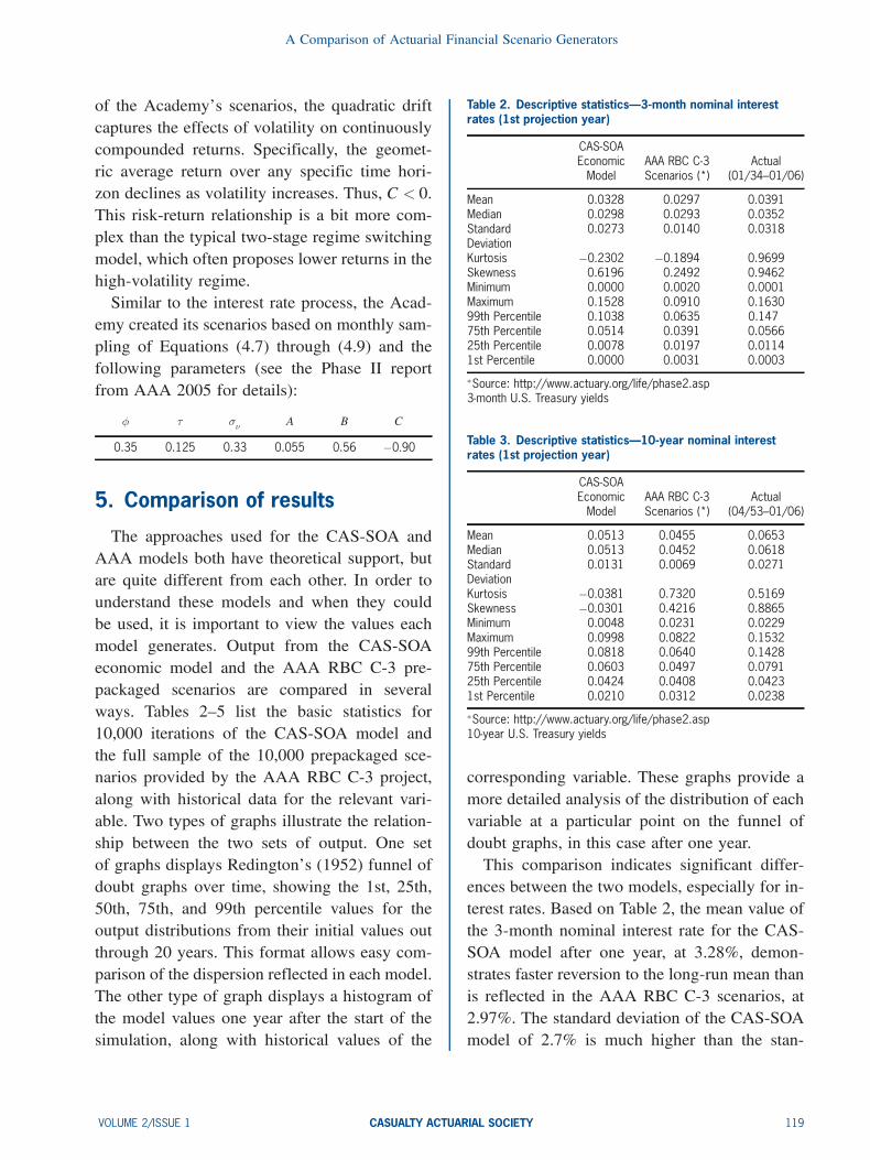
and dispersion for the 3-month nominal inter-est rate of the two models over a 20-year hori-zon. Both models start at approximately the same

level (CAS-SOA at 1.0% and the AAA at 1.21%),but the CAS-SOA model increases faster and to ahigher level with greater dispersion.2 Even after20 years, the AAA scenarios indicate a less than1% chance of 3-month interest rates exceeding13%, even though this value has been as highas 16% within the last 30 years. The histogramdisplayed in Figure 2 shows the distribution of 3-month nominal interest rates after one year. Thevalues for the AAA scenarios are almost entirelywithin the range of 1% to 5%. The CAS-SOAmodel has a much wider distribution, althoughnot as wide as the historical values.Comparing the results for the 10-year nomi-

nal interest rates produces a similar pattern. FromTable 3, the CAS-SOA values have a highermean, 5.1% to 4.6%, and standard deviation,1.3% to 0.7%, than the AAA scenarios. Actualvalues are only available for this data series from1953—2006, with a mean of 6.5%. Neither modelgenerates values for kurtosis or skewness that areclose to the limited period of historical valuesthat are available, but the signs of the AAA sce-narios are both positive, in line with actual val-ues. The funnel of doubt graphs in Figure 3 areboth higher and wider for the CAS-SOA valuesthan the AAA scenarios, except after 15 years.After this point, the AAA scenarios produce a99th percentile value above the values the CAS-SOA model produces, but the 50th and 75th per-centile values are still lower. Figure 4 shows thedistribution of the CAS-SOA model is wider thanthe AAA scenarios. Both are much lower thanthe historical values shown in the figure. How-ever, this discrepancy might not be a problem.Current interest rates, which are low by histori-cal standards, are used as the starting point forboth interest rate models. Despite mean rever-

2Immediately, readers may be drawn to the change in the slopeof the funnel of doubt graphs (Figures 1 and 3). This can be ex-plained by considering the time intervals illustrated in these graphs.The first half of these figures shows results at shorter (monthly)intervals. The second half of the figures indicates results at longerhorizons. The “kink” in the middle of these graphs reflects the shiftfrom monthly to annual intervals.



Figure 1. Funnel of doubt graphs: 3-month nominal interest rates

sion, high interest rates are less likely to occurwithin a year than they would be if interest rateswere starting at a higher level. However, fromJuly 1980 to July 1981, 10-year interest rates in-creased by 403 basis points, so the limited rangeof the AAA model might be considered too re-stricted.

Table 4 provides the basic statistics for largestock total returns for both models and for histor-ical values, based on the S&P 500 and its prede-cessor, the Cowles Index. The mean of the CAS-SOA model is 8.7%, and the mean for the AAAscenarios is 9.0%, both close to the historicalvalue of 10.4%. The standard deviation of the



Figure 2. Three-month nominal interest rates: model values and actual data (01/34–01/06)

CAS-SOA model, at 22.1%, is higher than theAAA scenarios, at 16.6%, and the historical val-ues, at 17.8%. The effect of the larger standarddeviation is evident in the 99th and 1st percentilevalues (largest 100 and smallest 100). These val-ues are 62.7% and ¡52:6% for the CAS-SOAmodel, but only 51.7% and ¡30:0% for the AAAscenarios. The AAA scenarios are in line withthe largest and smallest returns of the S&P 500(53.8% and ¡31:2%, respectively) over the 135-year period.The funnel of doubt graphs of Figure 5 nar-

row over time, rather than expand, due to theway stock returns are generated in the two mod-els. Stock return values represent the cumulativeaverage annual returns from investing in largestocks over the indicated time period. This pro-duces a portfolio effect over time, as large gainsor losses in one year are likely to be moderatedby the returns of the remaining years in the in-vestment horizon. Thus, the funnel of doubt isinverted, with returns more predictable for a 20-year investment horizon than for a single year.Since the standard deviation of returns is smaller

under the AAA approach, the compounded av-erage returns over longer periods converge morequickly. This difference is the result of the differ-ent approaches to the model, with the CAS-SOAmodel using regime switching and the AAAmodel based on the stochastic log volatilitymodel. The histogram in Figure 6 for large stockreturns after one year (which are measured sim-ilarly for both models) illustrate the similar dis-persion for the two models, both in line with ac-tual values.The results for small stock returns are indi-

cated in Table 5. In this case the CAS-SOA re-sults are closer to historical values. The meanvalue of the CAS-SOA model is 13.6%, com-pared with a mean of the AAA model of 10.3%and the historical mean of 17.5%. The standarddeviation of the CAS-SOA model, at 35.1%, iscloser than the AAA scenarios, at 22.6%, to thehistorical value of 33.1%. The 99th and 1st per-centile values are 129.7% and ¡61:8% for theCAS-SOA and 70.7% and ¡39:6% for the AAA.In this case the CAS-SOA results are closer to thehistorical range of 142.9% and ¡58:0% over a



Figure 3. Funnel of doubt graphs: 10-year nominal interest rates

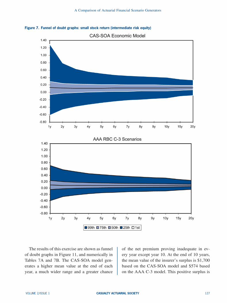
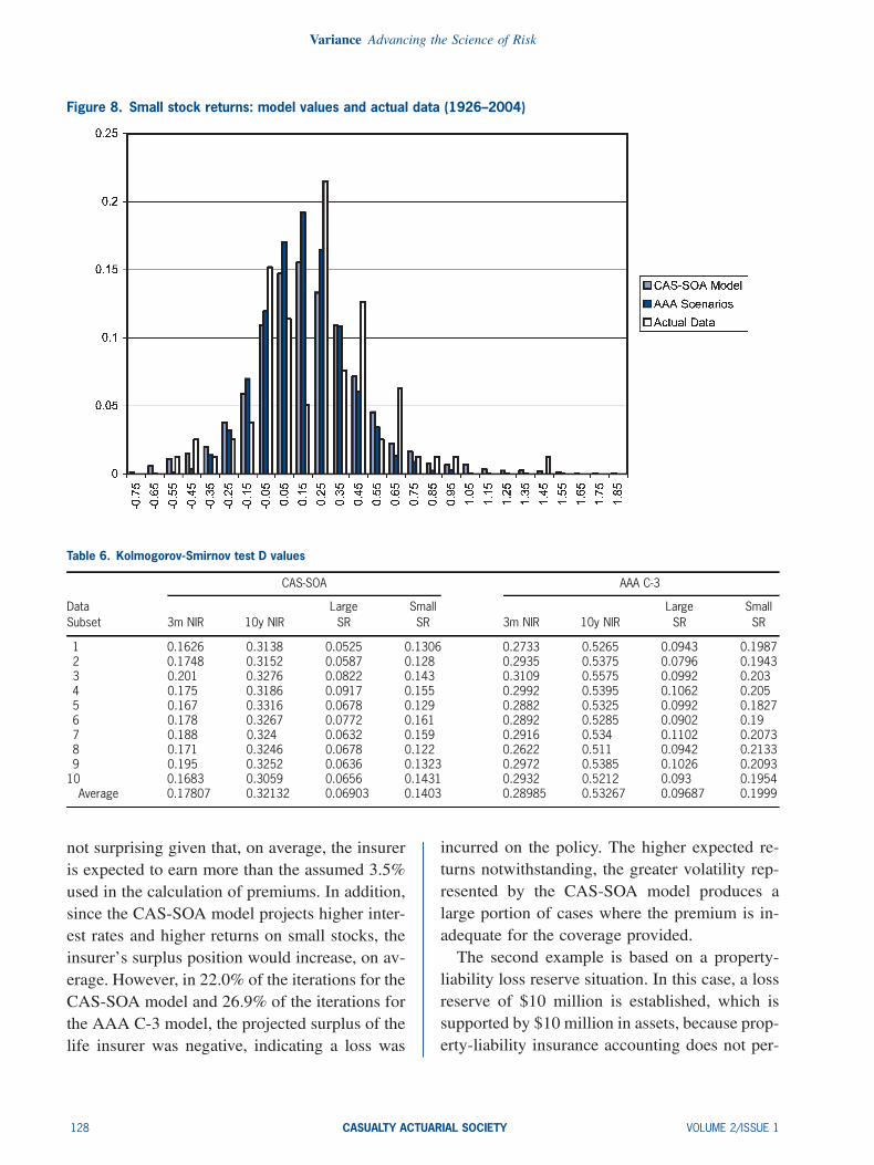
79-yearperiod.Thegreater initialdispersionof theCAS-SOA model is evident in Figure 7. The his-togram on Figure 8 provides another illustrationof the greater dispersion of the CAS-SOA model.Although the goal of each model is to pro-

vide a reasonable distribution of potential future

financial values, which cannot be quantified exante, it is possible to compare the output fromthe models to historical data to measure how wellthe models fit past experience. Two quantitativemetrics are used to test how closely the outputfrom the models conforms to historical values.



Figure 4. Ten-year nominal interest rates: model values and actual data (04/53–01/06)

The Kolmogorov-Smirnov (K-S) test measureswhether two datasets, in this case output fromeach model and actual observations, are signif-icantly different. This test does not depend onknowing the distribution of the underlying data,and therefore is not as sensitive as tests basedon specific distributions. The second test is thechi-square test that compares the distribution ofoutput from the model to the distribution of ac-tual observations.It should be noted that the models were not

developed solely to replicate history. Instead,the models are intended to provide a reasonableframework for understanding potential future un-certainty. Often, when choosing parameters foreconomic and financial models, users exploit his-torical relationships in time series data. Any teststatistic that measures historical fit is influencedby the weight given to past data. When param-eters are selected entirely from historical move-ments, statistical fit is likely to be affected. Inparticular, historical fit is likely to look better ifthere is significant overlap between the time pe-

riod used for parameter estimation and the timeperiod used to measure historical fit. Readersshould keep this in mind when looking at mea-sures of fit across competing models.The K-S test is illustrated graphically for 3-

month nominal interest rates in Figure 9. The cu-mulative distributions for historical interest ratesand both models (CAS-SOA and AAA) areshown. The K-S test metric D is the maximumvertical difference between the cumulative distri-bution of the actual data and cumulative distri-bution of each model. By comparing the D val-ues for the two models, we can determine whichmodel produces the better fit. Based on Figure9, the CAS-SOA model has a lower D and thusprovides a better fit to historical observations for3-month interest rates. In running this test, 10subsets of 1,000 observations each were drawnfrom the two models and the D values calcu-lated for each subset. The results are displayedin Table 6. For each variable, 3-month and 10-year interest rates and large and small stocks, theCAS-SOA model generated lower D values andtherefore produced a better fit.



Figure 5. Funnel of doubt graphs: large stock return (US equity)

Secondly, the chi-square method is used to testthe difference between the model output andactual values. The chi-square measure is thesquared difference between observed frequency(O) and the expected frequency (E), which isthen divided by the expected frequency. In this

case, observed frequency is the distribution ofhistorical interest rates or equity returns. Expect-ed frequency is the distribution of model val-ues from the underlying “known” distributionsas generated from CAS-SOA or AAA-C-3 mod-els. The sum of the differences between these



Figure 6. Large stock return: model values and actual data (1872–2006)

values from each of the multiple frequency inter-vals is the chi-square statistic, as shown in Equa-tion (5.1).

Â2 =X (O¡E)2

E: (5.1)

There are 42 bins based on 50 basis point in-tervals for interest rates and 17 bins (for largestocks) or 29 bins (for small stocks) based on 500basis point intervals for equity returns. The re-sults of chi-square test on both models are shownin Figure 10. For all cases the null hypothesis(that the model and observations are drawn fromthe same distribution) is rejected at the 10% level.However, the models do generate slightly differ-ent values for this metric. In general, the AAAmodel produces interest rates that correspondmore closely to historical distributions, whereasthe CAS-SOA model generates equity returnsthat correspond more closely with historical val-ues. The objective of the models, though, is toproject the potential distribution of future inter-est rates and equity returns, not to replicate dis-tributions of historical values.

6. Cash flow testingIn order to illustrate the differences between

the CAS-SOA financial scenario model and theAAA C-3 model, two simple examples are dem-onstrated here. The first example is a $100,000face value, single premium, ten-year term life in-surance policy for a 35-year-old male. The netpremium of $2,423 is determined by discount-ing the death benefits assuming 1980 CSO mor-tality rates and an interest rate of 3.5%. The sin-gle premium is invested in a portfolio that is al-located 50% to 3-month Treasury bills, 25% tolarge stocks, and 25% to small stocks. The in-vestment performance of each category is basedon 10,000 iterations of the competing financialmodels. At the end of each year, death benefitsare paid based on the assumed mortality table. Inthis simplified example, only the investment per-formance is assumed to be stochastic; a more re-alistic example would incorporate stochasticmortality rates, company expenses, and policycancellations. However, these situations are be-yond the scope of this project.



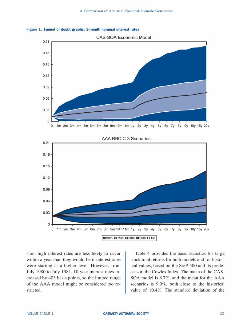
Figure 7. Funnel of doubt graphs: small stock return (intermediate risk equity)

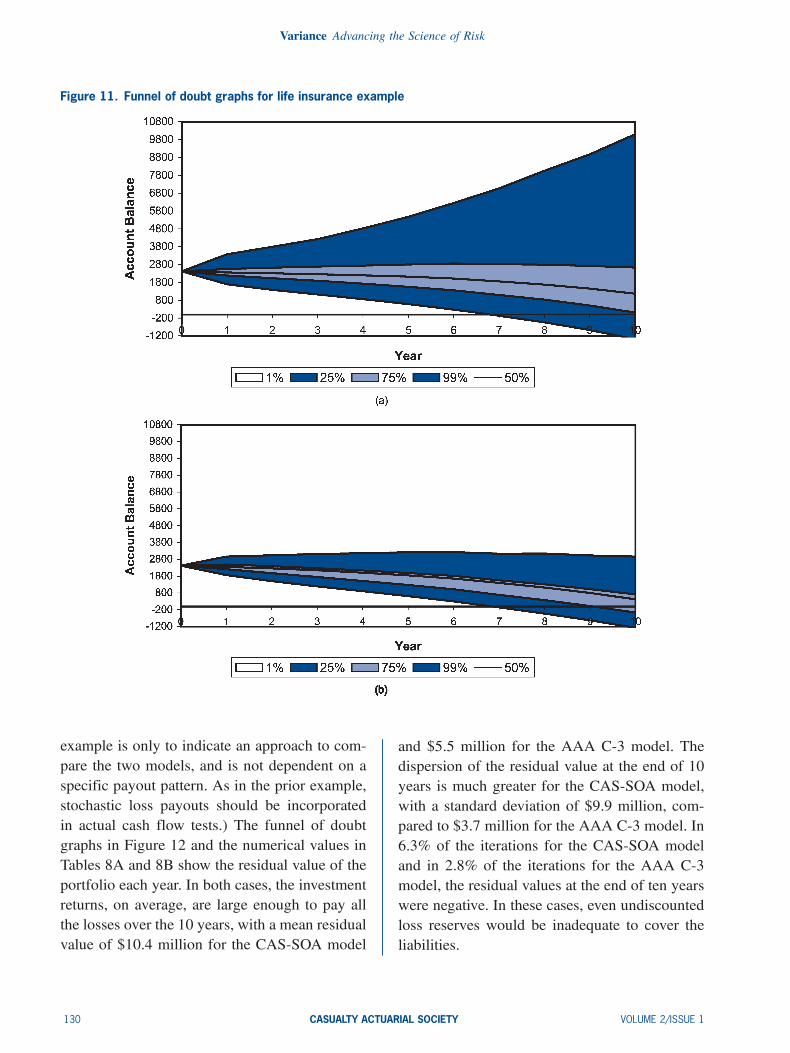
The results of this exercise are shown as funnelof doubt graphs in Figure 11, and numerically inTables 7A and 7B. The CAS-SOA model gen-erates a higher mean value at the end of eachyear, a much wider range and a greater chance

of the net premium proving inadequate in ev-ery year except year 10. At the end of 10 years,the mean value of the insurer’s surplus is $1,700based on the CAS-SOA model and $574 basedon the AAA C-3 model. This positive surplus is



Figure 8. Small stock returns: model values and actual data (1926–2004)

Table 6. Kolmogorov-Smirnov test D values

CAS-SOA AAA C-3

Data Large Small Large SmallSubset 3m NIR 10y NIR SR SR 3m NIR 10y NIR SR SR

1 0.1626 0.3138 0.0525 0.1306 0.2733 0.5265 0.0943 0.19872 0.1748 0.3152 0.0587 0.128 0.2935 0.5375 0.0796 0.19433 0.201 0.3276 0.0822 0.143 0.3109 0.5575 0.0992 0.2034 0.175 0.3186 0.0917 0.155 0.2992 0.5395 0.1062 0.2055 0.167 0.3316 0.0678 0.129 0.2882 0.5325 0.0992 0.18276 0.178 0.3267 0.0772 0.161 0.2892 0.5285 0.0902 0.197 0.188 0.324 0.0632 0.159 0.2916 0.534 0.1102 0.20738 0.171 0.3246 0.0678 0.122 0.2622 0.511 0.0942 0.21339 0.195 0.3252 0.0636 0.1323 0.2972 0.5385 0.1026 0.2093

10 0.1683 0.3059 0.0656 0.1431 0.2932 0.5212 0.093 0.1954Average 0.17807 0.32132 0.06903 0.1403 0.28985 0.53267 0.09687 0.1999

not surprising given that, on average, the insureris expected to earn more than the assumed 3.5%used in the calculation of premiums. In addition,since the CAS-SOA model projects higher inter-est rates and higher returns on small stocks, theinsurer’s surplus position would increase, on av-erage. However, in 22.0% of the iterations for theCAS-SOA model and 26.9% of the iterations forthe AAA C-3 model, the projected surplus of thelife insurer was negative, indicating a loss was

incurred on the policy. The higher expected re-turns notwithstanding, the greater volatility rep-resented by the CAS-SOA model produces alarge portion of cases where the premium is in-adequate for the coverage provided.The second example is based on a property-

liability loss reserve situation. In this case, a lossreserve of $10 million is established, which issupported by $10 million in assets, because prop-erty-liability insurance accounting does not per-



Table 7A. Projected surplus—life insurance example based on the CAS-SOA model

Year 1 2 3 4 5 6 7 8 9 10

Mean 2,381 2,351 2,326 2,302 2,270 2,219 2,120 2,017 1,877 1,700Median 2,357 2,315 2,260 2,200 2,127 2,016 1,856 1,678 1,450 1,170Standard Deviation 325 485 646 827 1,021 1,221 1,459 1,715 2,013 2,360Kurtosis 7.069 3.406 2.429 2.934 3.312 3.108 4.162 5.284 6.559 9.006Skewness 1.230 0.913 0.925 1.072 1.221 1.283 1.493 1.675 1.878 2.156Minimum 1,352 994 559 ,300 ¡15 ¡326 ¡724 ¡1,077 ¡1,687 ¡2,386Maximum 6,583 6,836 7,166 10,373 10,576 10,604 14,192 18,166 22,049 27,662# of Negative Values 0 0 0 0 1 14 142 534 1,254 2,20399th Percentile 3,371 3,793 4,222 4,824 5,473 6,247 7,061 8,045 8,970 10,09175th Percentile 2,550 2,620 2,682 2,739 2,803 2,852 2,823 2,792 2,722 2,63325th Percentile 2,184 2,031 1,889 1,730 1,554 1,356 1,094 834 507 1155th Percentile 1,905 1,637 1,404 1,163 911 660 317 ¡21 ¡417 ¡8871st Percentile 1,699 1,383 1,120 868 574 272 ¡77 ¡441 ¡872 ¡1,38510% TCE ¡942

Table 7B. Projected surplus—life insurance example based on the AAA C-3 model

Year 1 2 3 4 5 6 7 8 9 10

Mean 2,358 2,281 2,184 2,065 1,918 1,738 1,497 1,238 932 574Median 2,351 2,264 2,161 2,023 1,862 1,673 1,417 1,143 826 457Standard Deviation 225 321 401 476 547 614 680 747 813 879Kurtosis 0.747 0.358 0.486 0.624 0.670 0.884 1.272 1.439 1.649 1.944Skewness 0.323 0.341 0.422 0.535 0.618 0.704 0.807 0.875 0.936 0.997Minimum 1,479 1,276 1,001 787 494 203 ¡180 ¡553 ¡1,041 ¡1,610Maximum 3,563 3,687 3,963 4,700 4,688 5,063 5,730 5,600 5,782 6,371# of Negative Values 0 0 0 0 0 0 11 170 1,003 2,68699th Percentile 2,960 3,126 3,272 3,380 3,471 3,518 3,461 3,482 3,372 3,29675th Percentile 2,494 2,482 2,429 2,357 2,240 2,101 1,883 1,652 1,376 1,04625th Percentile 2,212 2,065 1,906 1,730 1,532 1,309 1,018 714 365 ¡395th Percentile 2,004 1,784 1,565 1,346 1,124 857 537 195 ¡189 ¡6241st Percentile 1,859 1,597 1,350 1,125 870 592 266 ¡87 ¡484 ¡94510% TCE ¡668

Figure 9. Three-month nominal interest rates: K-S testresults

mit discounting of loss reserves. The assets areinvested in the same portfolio used for the lifeinsurance example (50% 3-month Treasury bills,25% large stocks, and 25% small stocks). The

Figure 10. Chi-square test

loss payments are $1 million per year, paid atthe end of each year for 10 years. (More realisticloss payout patterns could be substituted for thisuniform set of payments, but the purpose of this



Figure 11. Funnel of doubt graphs for life insurance example

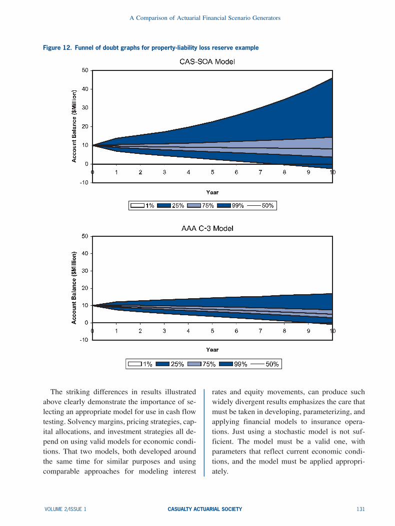
example is only to indicate an approach to com-pare the two models, and is not dependent on aspecific payout pattern. As in the prior example,stochastic loss payouts should be incorporatedin actual cash flow tests.) The funnel of doubtgraphs in Figure 12 and the numerical values inTables 8A and 8B show the residual value of theportfolio each year. In both cases, the investmentreturns, on average, are large enough to pay allthe losses over the 10 years, with a mean residualvalue of $10.4 million for the CAS-SOA model

and $5.5 million for the AAA C-3 model. Thedispersion of the residual value at the end of 10years is much greater for the CAS-SOA model,with a standard deviation of $9.9 million, com-pared to $3.7 million for the AAA C-3 model. In6.3% of the iterations for the CAS-SOA modeland in 2.8% of the iterations for the AAA C-3model, the residual values at the end of ten yearswere negative. In these cases, even undiscountedloss reserves would be inadequate to cover theliabilities.



Figure 12. Funnel of doubt graphs for property-liability loss reserve example

The striking differences in results illustratedabove clearly demonstrate the importance of se-lecting an appropriate model for use in cash flowtesting. Solvency margins, pricing strategies, cap-ital allocations, and investment strategies all de-pend on using valid models for economic condi-tions. That two models, both developed aroundthe same time for similar purposes and usingcomparable approaches for modeling interest

rates and equity movements, can produce suchwidely divergent results emphasizes the care thatmust be taken in developing, parameterizing, andapplying financial models to insurance opera-tions. Just using a stochastic model is not suf-ficient. The model must be a valid one, withparameters that reflect current economic condi-tions, and the model must be applied appropri-ately.



Table 8A. Property-liability loss reserve example based on the CAS-SOA model

Year 1 2 3 4 5 6 7 8 9 10

Mean 9.72 9.54 9.45 9.43 9.48 9.56 9.70 9.89 10.12 10.42Median 9.62 9.39 9.18 9.01 8.89 8.74 8.61 8.49 8.32 8.20Standard Deviation 1.34 1.99 2.64 3.38 4.17 5.00 6.00 7.09 8.39 9.92Kurtosis 7.07 3.44 2.44 2.95 3.33 3.10 4.15 5.23 6.45 8.82Skewness 1.23 0.92 0.93 1.08 1.22 1.28 1.49 1.67 1.87 2.14Minimum 5.48 3.97 2.23 1.26 0.14 ¡0:86 ¡1:95 ¡2:92 ¡4:06 ¡5:72Maximum 27.07 28.06 29.24 42.40 43.41 43.87 59.40 76.55 93.58 118.20# of Negative Values 0 0 0 0 0 5 32 131 321 63199th Percentile 13.81 15.49 17.22 19.72 22.60 26.05 30.04 34.49 39.61 46.0075th Percentile 10.42 10.65 10.91 11.22 11.65 12.17 12.60 13.10 13.70 14.4125th Percentile 8.91 8.23 7.66 7.10 6.55 6.02 5.49 4.99 4.39 3.695th Percentile 7.76 6.61 5.68 4.79 3.93 3.18 2.29 1.47 0.57 ¡0:391st Percentile 6.91 5.57 4.51 3.57 2.55 1.62 0.70 ¡0:28 ¡1:32 ¡2:3810% TCE ¡0:64

Table 8B. Property-liability loss reserve example based on the AAA C-3 model

Year 1 2 3 4 5 6 7 8 9 10

Mean 9.63 9.26 8.87 8.47 8.04 7.59 7.13 6.63 6.10 5.54Median 9.60 9.19 8.78 8.30 7.82 7.32 6.80 6.24 5.66 5.02Standard Deviation 0.93 1.32 1.64 1.95 2.24 2.52 2.80 3.09 3.39 3.69Kurtosis 0.75 0.36 0.49 0.63 0.67 0.88 1.27 1.44 1.65 1.97Skewness 0.32 0.34 0.42 0.54 0.62 0.70 0.81 0.88 0.94 1.01Minimum 6.00 5.14 4.04 3.26 2.23 1.32 0.20 ¡0:80 ¡1:84 ¡2:99Maximum 14.60 15.03 16.16 19.29 19.34 21.24 24.50 24.67 26.38 30.00# of Negative Values 0 0 0 0 0 0 0 10 72 28099th Percentile 12.11 12.74 13.32 13.84 14.40 14.91 15.20 15.98 16.36 16.8775th Percentile 10.19 10.09 9.87 9.66 9.36 9.08 8.72 8.36 7.95 7.5525th Percentile 9.02 8.37 7.74 7.10 6.46 5.84 5.16 4.45 3.73 2.955th Percentile 8.17 7.22 6.33 5.53 4.79 3.98 3.18 2.32 1.46 0.551st Percentile 7.57 6.45 5.45 4.63 3.76 2.90 2.06 1.15 0.14 ¡0:8410% TCE 0.36

7. Conclusions

Both the CAS-SOA model and the AAA pre-packaged scenarios provide values for interestrates and equity returns that can be used in ac-tuarial modeling. The different approaches usedin each procedure lead to significant differencesin the resulting output. The CAS-SOA modelleads to a wider set of distributions, especiallyfor interest rates, than the AAA scenarios. Beforeadopting either approach, the user should under-stand the factors considered by each model andhow their specific application may be affected bythe output.

ReferencesAhlgrim, K., S. P. D’Arcy, and R. W. Gorvett, “The Effec-tive Duration and Convexity of Liabilities for Property-Liability Insurers Under Stochastic Interest Rates,”Geneva Papers on Risk and Insurance Theory 29, 2004a,pp. 75—108.

Ahlgrim, K., S. P. D’Arcy, and R. W. Gorvett, “Report onModeling of Economic Series Coordinated with InterestRate Scenarios,” Arlington, VA: Casualty Actuarial So-ciety, 2004b, http://www.casact.org/research/econ/.

Ahlgrim, K., S. P. D’Arcy, and R. W. Gorvett, “ModelingFinancial Scenarios: A Framework for the Actuarial Pro-fession,” Proceedings of the Casualty Actuarial Society 92,2005, pp. 177—238.

American Academy of Actuaries, “Phase I Report of theAmerican Academy of Actuaries’ C-3 Subgroup of theLife Risk-Based Capital Task Force to the National As-sociation of Insurance Commissioners’ Risk-Based Cap-ital Work Group,” Washington, DC: American Academyof Actuaries, 1999, http://www.actuary.org/pdf/life/lrbcoctober.pdf.



AmericanAcademy ofActuaries, “RecommendedApproachfor Setting Regulatory Risk-Based Capital Requirementsfor Variable Products with Guarantees (Excluding IndexGuarantees),” Report of the Life Capital AdequacySubcommittee, Washington, DC: American Academyof Actuaries, 2002, http://www.actuary.org/pdf/life/rbc16dec02.pdf.

AmericanAcademy ofActuaries, “RecommendedApproachfor Setting Regulatory Risk-Based Capital Requirementsfor Variable Annuities and Similar Products,” Report ofthe Life Capital Adequacy Subcommittee, Washington,DC: American Academy of Actuaries, 2005, http://www.actuary.org/pdf/life/c3 june05.pdf.

D’Arcy, S. P., and R. W. Gorvett, “Measuring the InterestRate Sensitivity of Loss Reserves,” Proceedings of theCasualty Actuarial Society 87, 2000, pp. 365—400.

Fisher, I., Theory of Interest, New York: Macmillan, 1930.Hardy, M. R., “A Regime-Switching Model of Long-TermStock Returns,” North American Actuarial Journal 5 (2),2001, pp. 41—53, http://www.soa.org/library/naaj/1997-09/naaj0104 4.pdf.

Hibbert, J., P. Mowbray, and C. Turnbull, “A StochasticAsset Model and Calibration for Long-Term FinancialPlanning Purposes,” Technical Report, Edinburgh: Barrieand Hibbert, 2001.

Hull, J., Options, Futures, and Other Derivatives, Upper Sad-dle River, NJ: Prentice Hall, 2003.

Hull, J., and A. White, “Pricing Interest-Rate-Derivative Se-curities,” Review of Financial Studies 3, 1990, pp. 573—592.

Morris Commission, Morris Review of the Actuarial Profes-sion: Interim Assessment, Norwich, UK: HM Treasury,2004.

Redington, F. M., “Review of the Principles of Life OfficeValuations,” Journal of the Institute of Actuaries 78, 1952,pp. 1—40.

Vasicek, O., “An Equilibrium Characterization of the TermStructure,” Journal of Financial Economics 5, 1977, pp.177—188.

Wilkie, A. D., “A Stochastic Investment Model for ActuarialUse,” Transactions of the Faculty of Actuaries 39, 1986,pp. 341—403.

Wilkie, A. D., “More on a Stochastic Model for ActuarialUse,” British Actuarial Journal 1, 1995, pp. 777—964.

Appendix

List of Variables in Actuarial Scenario Genera-tors Panel A: CAS-SOA Model

Inflation Process

dqt = ·q(¹q¡ qt)dt+¾qdBq

qt Value of inflation at time t¹q Reversion level of inflation process

·q Speed of reversion

¾q Volatility of inflation process

Real Interest Rate Process

drt = ·1(lt¡ rt)dt+¾1dB1dlt = ·2(¹l¡ lt)dt+¾2dB2

rt Value of (instantaneous) real interest rateat time t

·1 Speed of reversion of real interest rate¾1 Volatility of real interest ratelt Value of reversion level of interest rate at

time t¹l Mean value of reversion level·2 Speed of reversion to mean value¾q Volatility of reversion level process

Equity Return Process

st = rt+ qt+ xt

lnxt j ½t »N(¹½t ,¾½t)

st (Total) equity return at time txt Excess equity return at time t (equity risk

premium)½t Regime at time t (½t = 1 or 2)List of Variables in Actuarial Scenario Genera-

tors Panel B: Academy Model

Interest Rate Process

d(ln`t) = ·`(μ`¡ ln`t)dt+ a't+ ºtdB`td't = ·'(μ'¡'t)dt+ b`t+¾'dB't

d(lnº2t ) = ·º(μº ¡ lnº2t )dt+¾ºdBºt

`t Value of long-term nominal interest rate attime t

μ` Reversion level of long-term rate process



·` Speed of reversion of long-term rateprocess

ºt Volatility of long-term rate process attime t

't Value of excess of short rate over longrate at time t

μ' Reversion level of spread process

·' Speed of reversion of spread process

¾' Volatility of spread process

μº Reversion level of long-term rate volatilityprocess

·º Speed of reversion of long-term ratevolatility process

¾º Volatility of long-term rate volatilityprocess

a, b Coefficients estimated from history

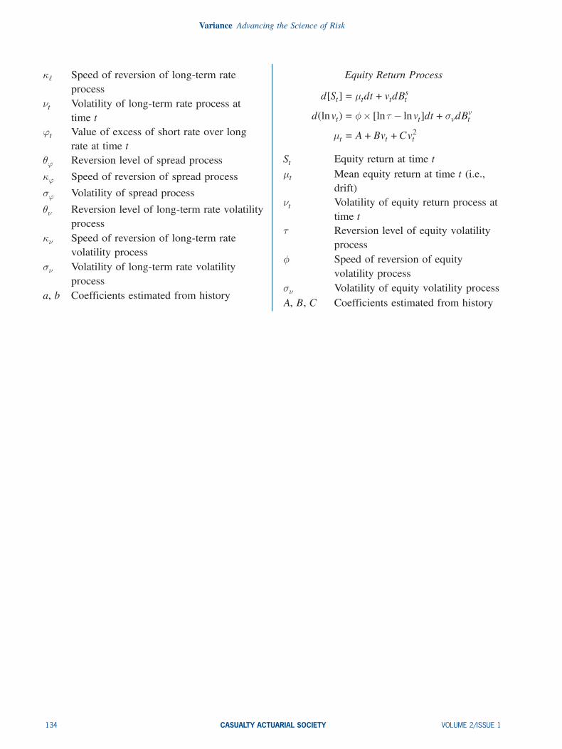
Equity Return Process

d[St] = ¹tdt+ vtdBst

d(lnvt) = Á£ [ln¿ ¡ lnvt]dt+¾vdBvt¹t = A+Bvt+Cv

2t

St Equity return at time t¹t Mean equity return at time t (i.e.,

drift)ºt Volatility of equity return process at

time t¿ Reversion level of equity volatility

processÁ Speed of reversion of equity

volatility process¾º Volatility of equity volatility processA, B, C Coefficients estimated from history


Documents

A Comparison of Actuarial Financial Scenario Generators - Variance