A Comparison of Edge Detectors in the Framework of Wake … · A Comparison of Edge Detectors in the Framework of Wake Pattern Modeling for Wind Turbines Yanjun Yan1, James Z. Zhang2,

A Comparison of Edge Detectors in the Framework of Wake PatternModeling for Wind Turbines

Yanjun Yan1, James Z. Zhang2, and Hayrettin Bora Karayaka3

1,3 Department of Engineering and Technology, Western Carolina University, Cullowhee, NC, 28723, [email protected]

[email protected]

2 Department of Electrical and Computer Engineering, Kettering University, Flint, MI, 48504, [email protected]

ABSTRACT

To monitor wind turbine health, wind farm operators can takeadvantage of the historical SCADA (supervisory control anddata acquisition) data to generate the wake pattern beforehandfor each wind turbine, and then decide in real time whetherobserved reduction in power generation is due to wake or truefaults. In our earlier efforts, we proposed an effective wakepattern modeling approach based on edge detector using Lin-ear Prediction (LP) with entropy-thresholding, and smoothingusing Empirical Mode Decomposition (EMD) on the windspeed difference plots. In this paper, we compare the LPbased edge detector with two other predominant edge detec-tors, Sobel and Canny edge detectors, to quantitatively justifythe appropriateness and effectiveness of the LP based edgedetector in wind turbine wake pattern analysis. We generatea fused wake model for the turbine of interest with multipleneighboring turbines, and then analyze the wake effect on tur-bine power generation. With a fused wake pattern, we do notneed to identify the individual source of wake any more. Weexpect that wakes cause reduced wind speed and hence re-duced power generation, but we have also observed from theSCADA data that the wind turbines in wake zones tend tooverreact when the wind speed is not yet close to the high-wind-shut-down threshold, which causes further power gen-eration loss.

1. INTRODUCTION

With the rapid development of the wind energy industry, themodern wind farms consist of hundreds of wind turbines.The effect of wake (Burton et al., 2001) is that, when a tur-

Yanjun Yan et al. This is an open-access article distributed under the terms ofthe Creative Commons Attribution 3.0 United States License, which permitsunrestricted use, distribution, and reproduction in any medium, provided theoriginal author and source are credited.

bine extracts energy from the wind, it leaves behind a wakecharacterized by reduced wind speeds and increased levels ofturbulence. Since wake adversely affects power generation,when a wind farm is being designed, the wind map informa-tion will be used to simulate the wake propagation for variousconfigurations of wind turbines. The optimal locationing ofthe wind turbines should enable the turbines to generate themost power in some windy locations while incurring the leastamount of wake. However, the co-existence of the large num-ber of turbines complicates the air dynamics, and the practicalconstraints (such as property ownerships, road building capa-bilities to transport and build the wind turbines) restrict wherethe wind turbines can be built. As a result, wake effect is un-avoidable at a certain wind direction for a certain turbine, al-though the likelihood is supposed to be minimized by properwind farm planning. When wake happens, the power gener-ation will be hampered. However, once the wind changes itsdirection and the downwind turbine is no longer in the wakeregion, the power generation will return to normal. There-fore, wake is not a fault of the wind turbine in itself, becausethe wind turbine can return to its full operational capacity assoon as it is no longer in wakes. Of course, while wake hap-pens, the air turbulence will stress the wind turbine more thannormal, which may lead to potential faults, but it is a grad-ual process, in a similar time scale as other wear and tear ef-fects. When we observe reduced power generation, we needto identify the wake effect to separate such temporary powerreduction from true faults.

There have been many efforts to model wake propagationacross the wind farm, mostly for wind farm design purposes(Ainslie, 1988; Quarton & Ainslie, 1990; Hassan, 1992; Wu& Port-Agel, 2011; Nilsson, 2012). Such models are moreaccurate over an averaging of 30 degree bins than across 5degree bins or 10 degree bins (Beaucage et al., 2012), be-cause the wake effect in a wider angular range may cancelout to yield a better overall power prediction accuracy. Once

International Journal of Prognostics and Health Management, ISSN2153-2648, 2015 028 1

INTERNATIONAL JOURNAL OF PROGNOSTICS AND HEALTH MANAGEMENT

the wind farms are built, the wake effects can be measuredby sodar (Barthelmie et al., 2006), lidar (Lang & McKeogh,2011), or remote sensing (Clive et al., 2012), in the entire at-mosphere of the wind farm. Arthelmie et al. (Barthelmie etal., 2006) compared several state-of-the-art theoretical wakemodels with the sodar measurements to discover that the spreadaway from the wake model predictions is considerable evenfor relatively simple offshore single wake cases. Recently,Philippe Beaucag et al. proposed the Deep-Array Wake Model(DAWM) that agrees with the real data better than other mod-els (such as Park (Jensen), Eddy Viscosity (Ainslie), and Com-putational Fluid Dynamics (CFD) models) for the offshorewind farms (Beaucage et al., 2012). For onshore applications,however, a better wake model is still of great interest in thewind energy community, particularly when the wake effect iscaused by multiple sources and complex terrains other thanthe sea surface.

Once the wind turbines are built and the wind farm is estab-lished, the main interest in wake analysis is for operationalmonitoring purpose. However, the models mentioned in theprevious paragraph are developed based on the physics ofair dynamics, often under simplified assumptions, and theycan not provide sufficiently fine resolution (Beaucage et al.,2012). Meanwhile, the models mentioned in the previousparagraph aim at estimating the entire wind farm’s powergeneration to help the investors decide whether they want tobuild the wind farm or not. Once the wind farm is built, thewake models should aim at estimating the individual windturbine’s power generation to help monitor the wind turbine’shealth and repair it in a timely fashion, if needed. A wakemodel using SCADA data is discussed in this paper, whichprovides an operational model of wake effects for each tur-bine of interest on the wind farm. Using the same frameworkbut individual data sets collected from each wind turbine, thegenerated wind pattern is customized for each wind turbine.This procedure is automatic and adaptive, which is desirablewhen handling a large number of wind turbines.

Yan et al. (Yan et al., 2009) proposed to model wake phe-nomena using SCADA data, where the major wake patternswere segmented using morphological imaging operators (di-lation and erosion) to automate the wake pattern identifica-tion. Then on the wake patterns, a threshold based deci-sion strategy was implemented to determine the existence ofwakes. However, the morphological operators were restrictedby the structuring element’s shape and size, and the bound-ary detected by the morphological operators could be im-proved. Meanwhile, the threshold based approach needs apriori knowledge on how much the wake effect would influ-ence the wind speed significantly, and such knowledge mightnot apply to different terrains. These issues were addressedin a recent paper (Yan & Zhang, 2014), where a solution ofmultiple steps was proposed: 1. In the wind speed differenceversus wind direction scatter plot, the data points within the

wake pattern might still be unconnected, and hence a movingwindow based intensity map was used to connect such sparsedata points. This intensity map was finer and more accuratethan using morphological operators in (Yan et al., 2009). 2.The “valleys” in the wake data represented the wake region’swidth and severity. An edge detector was used to capturethe characteristic pattern of the “valley”, based on the rel-ative depth calculated from the majority of the data, whichwas more adaptive than the threshold-based decision makerin (Yan et al., 2009). 3. A novel edge detector using LinearPrediction and Entropy Thresholding was used. The analysisin (Yan & Zhang, 2014) was qualitative without comprehen-sive comparison with other well-known edge detectors.

Therefore, the contributions of this paper include: 1. It presentsa comparison of the LP edge detector with Canny edge detec-tor and Sobel edge detector in the framework of wake patternmodeling. 2. It provides a comprehensive quantitative eval-uation of all these approaches. 3. It includes discussions onthe observations in wake pattern analysis and interpretationsof the observations in each wake zone.

The rest of the paper is organized as follows. The previouswork on wake pattern extraction is briefly explained in Sec-tion 2. The LP edge detector in this wake modeling frame-work is compared with other edge detectors in Section 3,where the properties of each approach are discussed. Sec-tion 4 demonstrates the wake pattern fusion of multiple neigh-boring turbines. Section 5 presents a metric to compare thethree approaches. Based on the best wake pattern, we parti-tion the data based on whether there is wake or not in Sec-tion 6, and interpret the data in Section 7. This paper is con-cluded in Section 8 with some future research areas identified.

2. WAKE REPRESENTATION AND INFORMATION EXTRAC-TION

In wind turbine’s operation, wind speed measurement is cru-cial, because wind speed is the input to the wind turbine’scontrol system, and the wind is the energy source that deter-mines how much power can be generated.

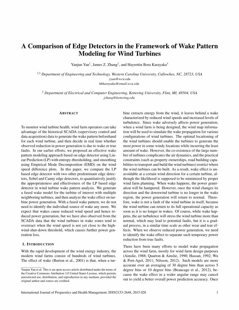
Figure 1. Compass coordinate to define the wind direction.

Wind direction is defined in the compass coordinate (US Deptof Commerce et al., 2002), as shown in Figure 1. In the wake

2


pattern, the x axis is the wind direction defined by Figure 1,the y axis is the normalized wind speed difference (Yan et al.,2009; Yan & Zhang, 2014) defined by

wsd =ws1 − ws2

(ws1 + ws2)/2= 2− 4

ws1/ws2 + 1, (1)

where ws1 is the wind speed of the 1st turbine (let say X),and ws2 is that of the 2nd turbine (let say Y ). The theoreti-cal data range of wsd is −2 to 2, but actual data range rarelygoes beyond −1 or 1. In wake analysis, we only care aboutthe negativewsd value when the current turbine is in the wakeof another turbine or obstruction , because the positive wsdvalue, when X blocks the wind to Y , is reflected in Y ’s wakepattern, and hence does not matter in X’s wake analysis. Theprominent features in this wake representation are the val-ley’s width (wake angular span) and depth (wake intensity).With hundreds of turbines on the wind farm, an automatedprocedure of wake pattern analysis is desirable, where imageprocessing is a handy tool to automate this procedure. Thesteps in this image processing procedure consist of intensitymap generation, edge detection, envelope extraction, and en-velope smoothing, to help estimate valley width and depth.

2.1. Intensity Map

Yan et al. proposed morphological imaging operators to seg-ment the majority of the data (Yan et al., 2009), but the pre-cision was limited by the shape and size of the structuringelements. To improve upon that approach and inspired by thefact that the data points were still sparse in the wake region(although much denser than the region with outliers), Yan andZhang proposed the intensity map, a moving window baseddata intensity measure (Yan & Zhang, 2014).

2.2. LP Based Edge Detection Method

Linear prediction (LP) uses a linear model to predict futurevalues of a discrete time signal using past and present values(Makhoul, 1975), while minimizing the the error between theestimated value and the real value. In images, however, edgescan be viewed as discontinuities in the given 2-D signal, andlarge errors in the estimated image represents the edge in-formation of that image (Zhang & Punch, 2012). After ap-plying the LP edge detection to an image, Yan and Zhangemployed an entropy-based threshold to further eliminate thebackground information and retain the edge information (Yan& Zhang, 2014; Zhang & Punch, 2012).

2.3. Envelope Extraction and Smoothing using EmpiricalMode Decomposition

Measurement of the valley width and the depth directly froman edge map is difficult given the irregular distribution ofedge pixels. It is desirable to convert the edge map into a“time-series like” data sequence so that standard mathemati-

cal techniques can be applied to calculate the span of a seg-ment as well as the extrema of the function. A lower envelopeof an edge map is extracted by simply keeping the minimalintensity value at each corresponding direction of the wake.The challenge is that there may be excessive ringing effectscaused by small variations in intensity around neighboringdirections. Consequently, appropriate smoothing needs to beapplied to the envelope to sufficiently remove ringing with-out significantly attenuate the amplitude. Due to its uniquefiltering characteristics, Yan and Zhang chose the EmpiricalMode Decomposition method (ur Rehman & Mandic, 2011)(Flandrin et al., 2004) (Huang et al., 1998) for smoothing.

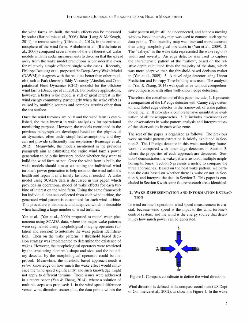
The basic concept of EMD is to identify proper time scalesthat reveals physical characteristics of the signals, and thendecompose the signal into modes intrinsic to the function,which are referred to as Intrinsic Mode Functions (IMF). Thefollowing signal is used as the input to the algorithm to ex-amine the output components for verification.

x(t) = sin(2.5πt) + 0.1 cos(50πt) + 0.8 sin(5πt) (2)

A signal defined in (2) is used as an example to show the pro-cedure of EMD in this waking modeling framework, becausethis signal contains various known frequency components andit looks like a typical envelope observed in wake pattern anal-ysis. The extracted IMFs are shown in figure 2 (a)-(c), whichillustrate that the amplitude and frequency contents of the sig-nal can be accurately extracted by EMD.

Figure 2. IMFs of x(t)

2.4. Wake Location and Severity Decision Maker

After the envelope of the scatter data is detected, the locationand information of the “valleys” are determined. Given anypoint on the envelope (the boundary points are considered ina circular fashion), if the points on its left and right are higherthan this point on the envelope, this point is considered a can-didate of valley point. The candidates of peak points canbe similarly identified. A segment of envelope with a val-ley point candidate in between two peak point candidates isconsidered an oscillation. The “valleys” are oscillations thatare significantly deeper than normal and are wide enough tobe substantial (Yan & Zhang, 2014). Meanwhile, the “smalldents” are consolidated into its neighboring “valleys” if thedents’ depth is small. The selected valleys’ depth indicates

3


the severity of the wakes, and the pixel breadth is convertedinto the corresponding angular width of the wakes.

3. COMPARISON WITH OTHER EDGE DETECTORS

The Canny edge detector (Canny, 1986) and Sobel edge de-tector (Farid & Simoncelli, 2004) are well established edgedetectors, and they could be used in place of the LP edge de-tector. However, one needs to understand the mechanism andthe purpose of the edge detector in our data processing to ap-preciate the differences in these edge detectors.

3.1. Sobel edge detector

The Sobel edge detector is one of the first-order differentia-tion based edge detectors (Belyaev, 2011), defined by

∆Ix =

−1 0 +1−2 0 +2−1 0 +1

· I (3)

∆Iy =

−1 −2 −10 0 0

+1 +2 +1

· I (4)

where I is an image, and its Sobel edge map is defined by

Iedge =√

∆I2x + ∆I2y (5)

3.2. Canny edge detector

The initial step in the Canny edge detector can be the Sobeledge detector (or other edge detectors), and then the pixelsthat are not within thin lines (regarded as not part of an edge)are removed (Canny, 1986). The Canny edge detector useshysteresis to declare a pixel, pd, with certain gradient value,d, to be an edge pixel (E(pd) = 1) or not (E(pd) = 0), basedon the following rule:

E(pd) =

0, if d < τl

1, if τl ≤ d ≤ τu and ∃E(neighbor(pd)) = 1

0, if τl ≤ d ≤ τu and ∀E(neighbor(pd)) = 0

1, if d > τu(6)

where τu is an upper threshold, τl is a lower threshold, anda typical ratio between τu and τl is between 2 : 1 and 3 : 1.When τl ≤ d ≤ τu, the pixel, pd, is declared an edge pixelonly if it is connected to another edge pixel.

3.3. Results when using different edge detectors

Wake pattern analysis includes edge map generation, enve-lope extraction, EMD smoothing, and deep “valley” charac-teristic derivation. The LP edge detector can be replaced bySobel and Canny edge detectors in this framework.

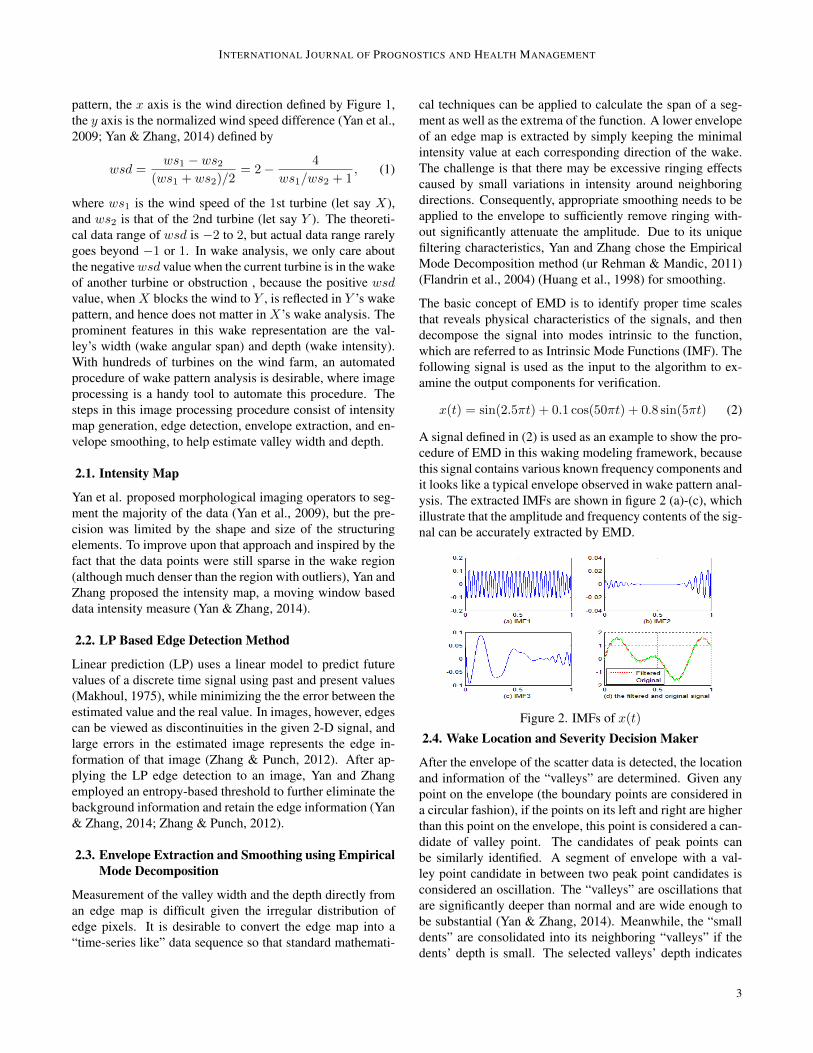
For a single turbine of interest with multiple neighboring tur-

bines, there are multiple wakes at different wind directions.Take real data as an example, turbine A is surrounded bytwelve other turbines within 1000 meter radius, as shown inFigure 3, which is an extraction from a much larger windfarm.

x (meter)0 200 400 600 800 1000 1200 1400 1600

y (m

eter

)

0

200

400

600

800

1000

1200

A B

1

2 3 4

5

6 7 8 9

10 11

Figure 3. All the turbines surrounding turbine A within a1000-meter radius.

The pair-wise wind speed difference versus wind directionplots are shown in Figures 4 and 5. The twelve pairs areshown in three blocks with four pairs in one block. The firstrow of each block shows the results from using LP edge de-tector, the second row using Sobel edge detector, and the thirdrow using Canny edge detectors. Each column is for a pair ofwind turbines. In each subplot, the x axis is the wind direc-tion in degrees (from 0 to 360), and the y axis is the normal-ized wind speed difference from -1 to 1 as defined in (1). Themagenta lines indicate the centers of the wakes.

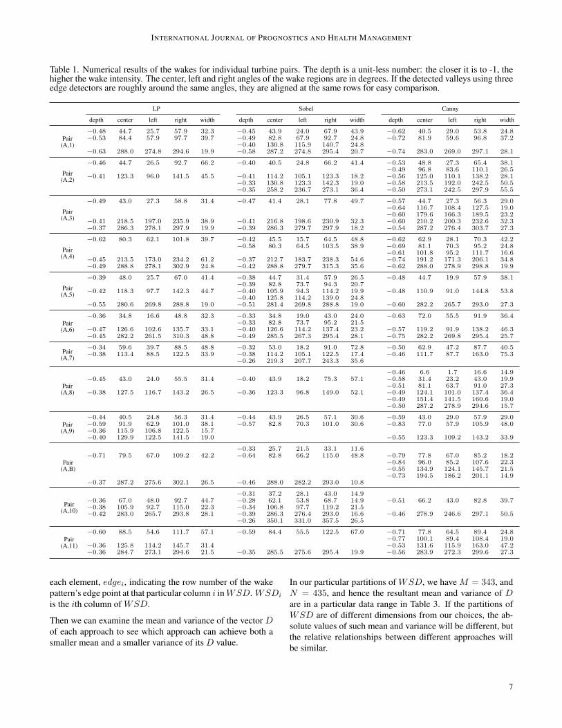
The numerical results showing the wake angle regions andthe intensity of the wake effect are listed in Table 1. Thedepth is a unit-less number: the closer it is to -1, the higherthe wake intensity. The center, left and right angles of thewake regions are in degrees. If the detected valleys usingthree edge detectors are roughly around the same angles, theyare aligned at the same rows for easy comparison.

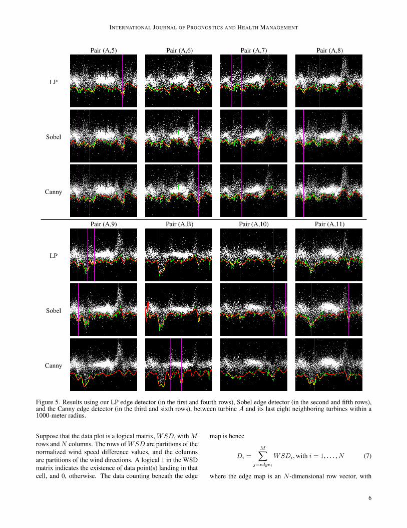
As observed, Sobel edge detector renders similar results tothose of the LP edge detector, but the edge extraction can beinaccurate to cause unnecessary oscillations and hence trivialwake regions, such as in Turbine pair (A, 5) in Figure 5. TheCanny edge detector renders some edges that are so low thatthey include outlier data points. Canny edge detector is anoptimal edge detector if the purpose is to extract objects froma natural scene (Canny, 1986), but given a scatter plot withpatches of different data densities, Canny edge detector is notas effective as a gradient based edge detector, such as Sobeledge detector and our LP edge detector. Another caveat to useSobel and Canny edge detectors is that when the envelope isspiky, the boundary condition in EMD smoothing may affectthe result, as shown in the Sobel pair (A,B) in Figure 5, andCanny edge detector’s Sim IDW fusion result in Figure 6.

4


4. FUSION FOR A COMPREHENSIVE WAKE PATTERN

A complete understanding of the wake pattern of a centralturbine demands an analysis from all of its neighbors, such asin Figures 4 and 5. The individual pairs’ results are furtherfused by the four schemes (Yan et al., 2009):

1. Equal-weight fusion (EW), where all data scatters arecombined with equal weight.

2. Inverse-distance-weight fusion (IDW), where the data scat-ters are combined with heavier weight on the closer neigh-bors.

3. Similarity clustering based EW fusion (Sim EW), wherethe similar clusters are fused first, and the clusters aretreated equally.

4. Similarity clustering based IDW fusion (Sim IDW), wherethe clusters are weighted based on their distances to thecentering turbine.

The numerical results showing the fused wake patterns usingthe proposed framework and the comparison of three edgedetectors are listed in Table 2.

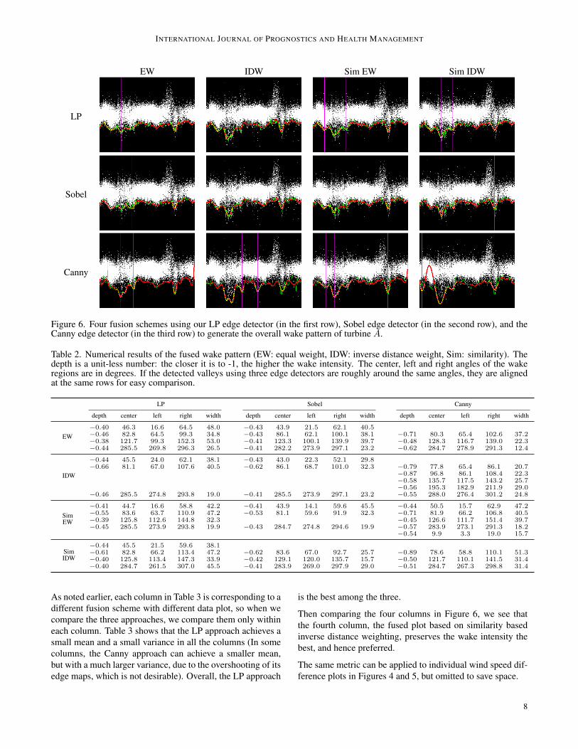
Figure 6 shows the fused wake pattern using the LP edge de-tector, the Sobel edge detector, and the Canny edge detector.The similarity-clustering based fusion preserves the wake in-tensity information better than the ones without clustering,and the equal-weight based fusion turns out to be more ro-bust than the inverse-distance-weight scheme, which further

indicates that distance alone is not necessarily a stable indi-cator of wake intensity.

As mentioned earlier, Sobel and Canny edge maps can bespikier than LP edge map, yielding harder constraints on theboundary conditions for the EMD procedure to cause unde-sired smoothing results, such as in the right-most plot in thelast row in Figure 6, where the filtered envelope using Cannyedge detector fails to follow the edge map in certain segments.This did not happen for LP edge detector in our experiments,because LP edge detector uses entropy thresholding to effec-tively adjust its edge declaration threshold for each plot.

5. A METRIC TO EVALUATE THE WAKE PATTERN

To quantify the goodness of an approach to derive the wakepattern, we propose a numerical metric, besides the analysisearlier. The desired property of such a metric is that the de-rived wake pattern should follow the data accurately. Namely,the data points beneath the smoothed edge map should be rea-sonable few, with low density.

Take Figure 6 as an example: In each column of subplots,the same fused data plot is fed into the wake pattern analysissystem. Depending on the choice of edge detector, the edgemap is different. Different columns use different fused data.While comparing different edge detectors, we focus on eachcolumn of Figure 6.

Pair (A,1) Pair (A,2) Pair (A,3) Pair (A,4)

LP

Sobel

Canny

Figure 4. Results using our LP edge detector (in the first row), Sobel edge detector (in the second row), and the Canny edgedetector (in the third row), between turbineA and its first four neighboring turbines within a 1000-meter radius. In each subplotof this figure and the next two figures, the x axis is the wind direction in degrees (from 0 to 360), and the y axis is the normalizedwind speed difference from -1 to 1 as defined in (1).

5


Pair (A,5) Pair (A,6) Pair (A,7) Pair (A,8)

LP

Sobel

Canny

Pair (A,9) Pair (A,B) Pair (A,10) Pair (A,11)

LP

Sobel

Canny

Figure 5. Results using our LP edge detector (in the first and fourth rows), Sobel edge detector (in the second and fifth rows),and the Canny edge detector (in the third and sixth rows), between turbine A and its last eight neighboring turbines within a1000-meter radius.

Suppose that the data plot is a logical matrix, WSD, with Mrows andN columns. The rows ofWSD are partitions of thenormalized wind speed difference values, and the columnsare partitions of the wind directions. A logical 1 in the WSDmatrix indicates the existence of data point(s) landing in thatcell, and 0, otherwise. The data counting beneath the edge

map is hence

Di =

M∑j=edgei

WSDi,with i = 1, . . . , N (7)

where the edge map is an N -dimensional row vector, with

6


Table 1. Numerical results of the wakes for individual turbine pairs. The depth is a unit-less number: the closer it is to -1, thehigher the wake intensity. The center, left and right angles of the wake regions are in degrees. If the detected valleys using threeedge detectors are roughly around the same angles, they are aligned at the same rows for easy comparison.

LP Sobel Canny

depth center left right width depth center left right width depth center left right width

Pair(A,1)

−0.48 44.7 25.7 57.9 32.3 −0.45 43.9 24.0 67.9 43.9 −0.62 40.5 29.0 53.8 24.8−0.53 84.4 57.9 97.7 39.7 −0.49 82.8 67.9 92.7 24.8 −0.72 81.9 59.6 96.8 37.2

−0.40 130.8 115.9 140.7 24.8−0.63 288.0 274.8 294.6 19.9 −0.58 287.2 274.8 295.4 20.7 −0.74 283.0 269.0 297.1 28.1

Pair(A,2)

−0.46 44.7 26.5 92.7 66.2 −0.40 40.5 24.8 66.2 41.4 −0.53 48.8 27.3 65.4 38.1−0.49 96.8 83.6 110.1 26.5

−0.41 123.3 96.0 141.5 45.5 −0.41 114.2 105.1 123.3 18.2 −0.56 125.0 110.1 138.2 28.1−0.33 130.8 123.3 142.3 19.0 −0.58 213.5 192.0 242.5 50.5−0.35 258.2 236.7 273.1 36.4 −0.50 273.1 242.5 297.9 55.5

Pair(A,3)

−0.49 43.0 27.3 58.8 31.4 −0.47 41.4 28.1 77.8 49.7 −0.57 44.7 27.3 56.3 29.0−0.64 116.7 108.4 127.5 19.0−0.60 179.6 166.3 189.5 23.2

−0.41 218.5 197.0 235.9 38.9 −0.41 216.8 198.6 230.9 32.3 −0.60 210.2 200.3 232.6 32.3−0.37 286.3 278.1 297.9 19.9 −0.39 286.3 279.7 297.9 18.2 −0.54 287.2 276.4 303.7 27.3

Pair(A,4)

−0.62 80.3 62.1 101.8 39.7 −0.42 45.5 15.7 64.5 48.8 −0.62 62.9 28.1 70.3 42.2−0.58 80.3 64.5 103.5 38.9 −0.69 81.1 70.3 95.2 24.8

−0.61 101.8 95.2 111.7 16.6−0.45 213.5 173.0 234.2 61.2 −0.37 212.7 183.7 238.3 54.6 −0.74 191.2 171.3 206.1 34.8−0.49 288.8 278.1 302.9 24.8 −0.42 288.8 279.7 315.3 35.6 −0.62 288.0 278.9 298.8 19.9

Pair(A,5)

−0.39 48.0 25.7 67.0 41.4 −0.38 44.7 31.4 57.9 26.5 −0.48 44.7 19.9 57.9 38.1−0.39 82.8 73.7 94.3 20.7

−0.42 118.3 97.7 142.3 44.7 −0.40 105.9 94.3 114.2 19.9 −0.48 110.9 91.0 144.8 53.8−0.40 125.8 114.2 139.0 24.8

−0.55 280.6 269.8 288.8 19.0 −0.51 281.4 269.8 288.8 19.0 −0.60 282.2 265.7 293.0 27.3

Pair(A,6)

−0.36 34.8 16.6 48.8 32.3 −0.33 34.8 19.0 43.0 24.0 −0.63 72.0 55.5 91.9 36.4−0.33 82.8 73.7 95.2 21.5

−0.47 126.6 102.6 135.7 33.1 −0.40 126.6 114.2 137.4 23.2 −0.57 119.2 91.9 138.2 46.3−0.45 282.2 261.5 310.3 48.8 −0.49 285.5 267.3 295.4 28.1 −0.75 282.2 269.8 295.4 25.7

Pair(A,7)

−0.34 59.6 39.7 88.5 48.8 −0.32 53.0 18.2 91.0 72.8 −0.50 62.9 47.2 87.7 40.5−0.38 113.4 88.5 122.5 33.9 −0.38 114.2 105.1 122.5 17.4 −0.46 111.7 87.7 163.0 75.3

−0.26 219.3 207.7 243.3 35.6

Pair(A,8)

−0.46 6.6 1.7 16.6 14.9−0.45 43.0 24.0 55.5 31.4 −0.40 43.9 18.2 75.3 57.1 −0.58 31.4 23.2 43.0 19.9

−0.51 81.1 63.7 91.0 27.3−0.38 127.5 116.7 143.2 26.5 −0.36 123.3 96.8 149.0 52.1 −0.49 124.1 101.0 137.4 36.4

−0.49 151.4 141.5 160.6 19.0−0.50 287.2 278.9 294.6 15.7

Pair(A,9)

−0.44 40.5 24.8 56.3 31.4 −0.44 43.9 26.5 57.1 30.6 −0.59 43.0 29.0 57.9 29.0−0.59 91.9 62.9 101.0 38.1 −0.57 82.8 70.3 101.0 30.6 −0.83 77.0 57.9 105.9 48.0−0.36 115.9 106.8 122.5 15.7−0.40 129.9 122.5 141.5 19.0 −0.55 123.3 109.2 143.2 33.9

Pair(A,B)

−0.33 25.7 21.5 33.1 11.6−0.71 79.5 67.0 109.2 42.2 −0.64 82.8 66.2 115.0 48.8 −0.79 77.8 67.0 85.2 18.2

−0.84 96.0 85.2 107.6 22.3−0.55 134.9 124.1 145.7 21.5−0.73 194.5 186.2 201.1 14.9

−0.37 287.2 275.6 302.1 26.5 −0.46 288.0 282.2 293.0 10.8

Pair(A,10)

−0.31 37.2 28.1 43.0 14.9−0.36 67.0 48.0 92.7 44.7 −0.28 62.1 53.8 68.7 14.9 −0.51 66.2 43.0 82.8 39.7−0.38 105.9 92.7 115.0 22.3 −0.34 106.8 97.7 119.2 21.5−0.42 283.0 265.7 293.8 28.1 −0.39 286.3 276.4 293.0 16.6 −0.46 278.9 246.6 297.1 50.5

−0.26 350.1 331.0 357.5 26.5

Pair(A,11)

−0.60 88.5 54.6 111.7 57.1 −0.59 84.4 55.5 122.5 67.0 −0.71 77.8 64.5 89.4 24.8−0.77 100.1 89.4 108.4 19.0

−0.36 125.8 114.2 145.7 31.4 −0.53 131.6 115.9 163.0 47.2−0.36 284.7 273.1 294.6 21.5 −0.35 285.5 275.6 295.4 19.9 −0.56 283.9 272.3 299.6 27.3

each element, edgei, indicating the row number of the wakepattern’s edge point at that particular column i inWSD. WSDi

is the ith column of WSD.

Then we can examine the mean and variance of the vector Dof each approach to see which approach can achieve both asmaller mean and a smaller variance of its D value.

In our particular partitions of WSD, we have M = 343, andN = 435, and hence the resultant mean and variance of Dare in a particular data range in Table 3. If the partitions ofWSD are of different dimensions from our choices, the ab-solute values of such mean and variance will be different, butthe relative relationships between different approaches willbe similar.

7


EW IDW Sim EW Sim IDW

LP

Sobel

Canny

Figure 6. Four fusion schemes using our LP edge detector (in the first row), Sobel edge detector (in the second row), and theCanny edge detector (in the third row) to generate the overall wake pattern of turbine A.

Table 2. Numerical results of the fused wake pattern (EW: equal weight, IDW: inverse distance weight, Sim: similarity). Thedepth is a unit-less number: the closer it is to -1, the higher the wake intensity. The center, left and right angles of the wakeregions are in degrees. If the detected valleys using three edge detectors are roughly around the same angles, they are alignedat the same rows for easy comparison.

LP Sobel Canny

depth center left right width depth center left right width depth center left right width

EW−0.40 46.3 16.6 64.5 48.0 −0.43 43.9 21.5 62.1 40.5−0.46 82.8 64.5 99.3 34.8 −0.43 86.1 62.1 100.1 38.1 −0.71 80.3 65.4 102.6 37.2−0.38 121.7 99.3 152.3 53.0 −0.41 123.3 100.1 139.9 39.7 −0.48 128.3 116.7 139.0 22.3−0.44 285.5 269.8 296.3 26.5 −0.41 282.2 273.9 297.1 23.2 −0.62 284.7 278.9 291.3 12.4

IDW

−0.44 45.5 24.0 62.1 38.1 −0.43 43.0 22.3 52.1 29.8−0.66 81.1 67.0 107.6 40.5 −0.62 86.1 68.7 101.0 32.3 −0.79 77.8 65.4 86.1 20.7

−0.87 96.8 86.1 108.4 22.3−0.58 135.7 117.5 143.2 25.7−0.56 195.3 182.9 211.9 29.0

−0.46 285.5 274.8 293.8 19.0 −0.41 285.5 273.9 297.1 23.2 −0.55 288.0 276.4 301.2 24.8

SimEW

−0.41 44.7 16.6 58.8 42.2 −0.41 43.9 14.1 59.6 45.5 −0.44 50.5 15.7 62.9 47.2−0.55 83.6 63.7 110.9 47.2 −0.53 81.1 59.6 91.9 32.3 −0.71 81.9 66.2 106.8 40.5−0.39 125.8 112.6 144.8 32.3 −0.45 126.6 111.7 151.4 39.7−0.45 285.5 273.9 293.8 19.9 −0.43 284.7 274.8 294.6 19.9 −0.57 283.9 273.1 291.3 18.2

−0.54 9.9 3.3 19.0 15.7

SimIDW

−0.44 45.5 21.5 59.6 38.1−0.61 82.8 66.2 113.4 47.2 −0.62 83.6 67.0 92.7 25.7 −0.89 78.6 58.8 110.1 51.3−0.40 125.8 113.4 147.3 33.9 −0.42 129.1 120.0 135.7 15.7 −0.50 121.7 110.1 141.5 31.4−0.40 284.7 261.5 307.0 45.5 −0.41 283.9 269.0 297.9 29.0 −0.51 284.7 267.3 298.8 31.4

As noted earlier, each column in Table 3 is corresponding to adifferent fusion scheme with different data plot, so when wecompare the three approaches, we compare them only withineach column. Table 3 shows that the LP approach achieves asmall mean and a small variance in all the columns (In somecolumns, the Canny approach can achieve a smaller mean,but with a much larger variance, due to the overshooting of itsedge maps, which is not desirable). Overall, the LP approach

is the best among the three.

Then comparing the four columns in Figure 6, we see thatthe fourth column, the fused plot based on similarity basedinverse distance weighting, preserves the wake intensity thebest, and hence preferred.

The same metric can be applied to individual wind speed dif-ference plots in Figures 4 and 5, but omitted to save space.

8


Table 3. The mean and variance comparison of metric D (agood approach achieves both small µ and small σ). Each col-umn is corresponding to a different fused data set, so the com-parison is within each column.

µ EW IDW Sim EW Sim IDWLP 1.7678 2.1195 1.8391 1.9011

Sobel 2.2552 3.2069 2.2161 2.4483Canny 1.292 0.7839 1.2552 5.308

σ EW IDW Sim EW Sim IDWLP 3.3354 3.7368 3.3105 3.4626

Sobel 4.8172 7.123 3.8933 4.5751Canny 47.6035 15.308 33.1721 283.3565

6. DATA PARTITION BASED ON THE WAKE PATTERN

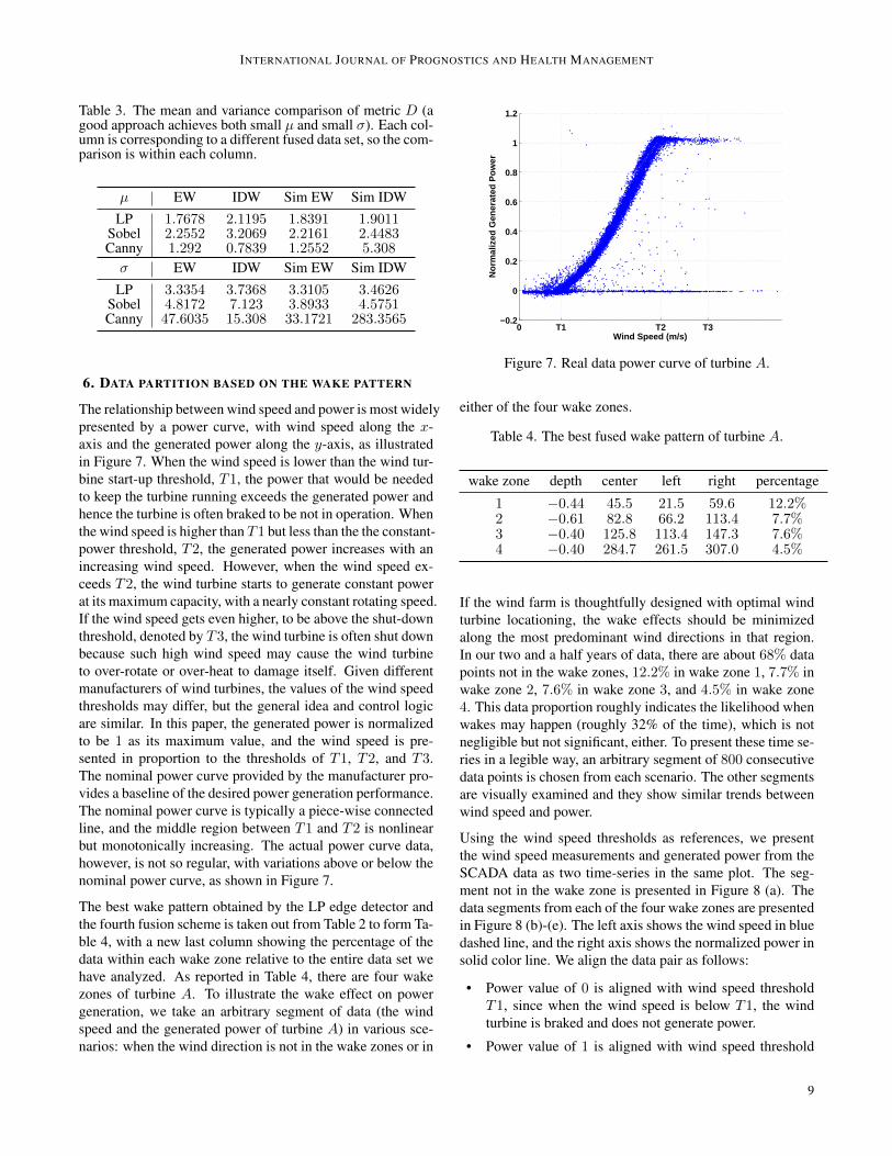
The relationship between wind speed and power is most widelypresented by a power curve, with wind speed along the x-axis and the generated power along the y-axis, as illustratedin Figure 7. When the wind speed is lower than the wind tur-bine start-up threshold, T1, the power that would be neededto keep the turbine running exceeds the generated power andhence the turbine is often braked to be not in operation. Whenthe wind speed is higher than T1 but less than the the constant-power threshold, T2, the generated power increases with anincreasing wind speed. However, when the wind speed ex-ceeds T2, the wind turbine starts to generate constant powerat its maximum capacity, with a nearly constant rotating speed.If the wind speed gets even higher, to be above the shut-downthreshold, denoted by T3, the wind turbine is often shut downbecause such high wind speed may cause the wind turbineto over-rotate or over-heat to damage itself. Given differentmanufacturers of wind turbines, the values of the wind speedthresholds may differ, but the general idea and control logicare similar. In this paper, the generated power is normalizedto be 1 as its maximum value, and the wind speed is pre-sented in proportion to the thresholds of T1, T2, and T3.The nominal power curve provided by the manufacturer pro-vides a baseline of the desired power generation performance.The nominal power curve is typically a piece-wise connectedline, and the middle region between T1 and T2 is nonlinearbut monotonically increasing. The actual power curve data,however, is not so regular, with variations above or below thenominal power curve, as shown in Figure 7.

The best wake pattern obtained by the LP edge detector andthe fourth fusion scheme is taken out from Table 2 to form Ta-ble 4, with a new last column showing the percentage of thedata within each wake zone relative to the entire data set wehave analyzed. As reported in Table 4, there are four wakezones of turbine A. To illustrate the wake effect on powergeneration, we take an arbitrary segment of data (the windspeed and the generated power of turbine A) in various sce-narios: when the wind direction is not in the wake zones or in

0 T1 T2 T3−0.2

0

0.2

0.4

0.6

0.8

1

1.2

Wind Speed (m/s)

Nor

mal

ized

Gen

erat

ed P

ower

Figure 7. Real data power curve of turbine A.

either of the four wake zones.

Table 4. The best fused wake pattern of turbine A.

wake zone depth center left right percentage

1 −0.44 45.5 21.5 59.6 12.2%2 −0.61 82.8 66.2 113.4 7.7%3 −0.40 125.8 113.4 147.3 7.6%4 −0.40 284.7 261.5 307.0 4.5%

If the wind farm is thoughtfully designed with optimal windturbine locationing, the wake effects should be minimizedalong the most predominant wind directions in that region.In our two and a half years of data, there are about 68% datapoints not in the wake zones, 12.2% in wake zone 1, 7.7% inwake zone 2, 7.6% in wake zone 3, and 4.5% in wake zone4. This data proportion roughly indicates the likelihood whenwakes may happen (roughly 32% of the time), which is notnegligible but not significant, either. To present these time se-ries in a legible way, an arbitrary segment of 800 consecutivedata points is chosen from each scenario. The other segmentsare visually examined and they show similar trends betweenwind speed and power.

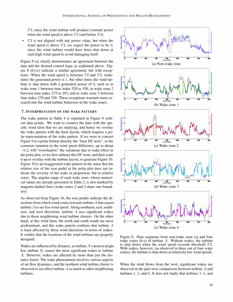
Using the wind speed thresholds as references, we presentthe wind speed measurements and generated power from theSCADA data as two time-series in the same plot. The seg-ment not in the wake zone is presented in Figure 8 (a). Thedata segments from each of the four wake zones are presentedin Figure 8 (b)-(e). The left axis shows the wind speed in bluedashed line, and the right axis shows the normalized power insolid color line. We align the data pair as follows:

• Power value of 0 is aligned with wind speed thresholdT1, since when the wind speed is below T1, the windturbine is braked and does not generate power.

• Power value of 1 is aligned with wind speed threshold

9


T2, since the wind turbine will produce constant powerwhen the wind speed is above T2 (and below T3).

• T3 is not aligned with any power value, but when thewind speed is above T3, we expect the power to be 0,since the wind turbine would have been shut down atsuch high wind speed to avoid damaging itself.

Figure 8 (a) clearly demonstrates an agreement between thedata and the desired control logic as explained above. Fig-ure 8 (b)-(e) indicate a similar agreement, but with excep-tions: When the wind speed is between T2 and T3, some-times the generated power is 1, but other times the wind tur-bine is shut down with a generated power of 0, such as inwake zone 1 between time index 520 to 550, in wake zone 2between time index 275 to 293, and in wake zone 3 betweentime index 278 and 329. These exceptions warrants more re-search into the wind turbine behaviors in the wake zones.

7. INTERPRETATION OF THE WAKE PATTERN

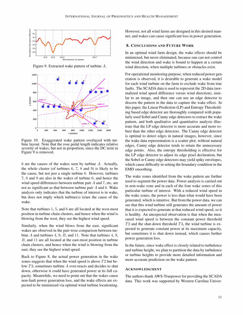
The wake pattern in Table 4 is replotted in Figure 9 with-out data points. We want to connect the data with the spe-cific wind farm that we are studying, and hence we overlaythe wake pattern with the farm layout, which requires a po-lar representation of the wake pattern. If we were to convertFigure 9 to a polar format directly, the “base DC term”, or thecommon variation in the wind speed difference, up to about−0.2, will “overshadow” the variations due to wake effect inthe polar plot, so we first subtract this DC term, and then scaleit up to overlay with the turbine layout, to generate Figure 10.Figure 10 is an exaggerated wake pattern in the sense that therelative size of the rose pedal in the polar plot does not in-dicate the severity of the wake in proportion, but in relativesense. The angular range of each wake zone, whose numeri-cal values are already presented in Table 2, is also marked bymagenta dashed lines (wake zones 2 and 3 share one bound-ary).

As observed from Figure 10, the rose pedals indicate the di-rections from which wind comes towards turbineA that causesturbineA to see less wind speed. Along northeast, east, south-east, and west directions, turbine A sees significant wakesdue to those neighboring wind turbine clusters. On the otherhand, at this wind farm, the north and south winds are mostpredominant, and this wake pattern confirms that turbine Ais least affected by those wind directions in terms of wakes.It verifies that the locations of the wind turbines are properlydesigned.

Wakes are influenced by distance, as turbineA’s nearest neigh-bor, turbine B, causes the most significant wakes to turbineA. However, wakes are affected by more than just the dis-tance factor. The wake phenomenon involves various aspectsof air flow dynamics, and the northern wind turbine cluster isobserved to not affect turbineA as much as other neighboringturbines.

0 100 200 300 400 500 600 700 8000

T1

T2

T3

Win

d S

pee

d (

m/s

)

0 100 200 300 400 500 600 700 800

0

1

No

rmal

ized

Gen

erat

ed P

ow

er

Time Index

(a) Non-wake zone

0 100 200 300 400 500 600 700 8000

T1

T2

T3

Win

d S

pee

d (

m/s

)

0 100 200 300 400 500 600 700 800

0

1

No

rmal

ized

Gen

erat

ed P

ow

er

Time Index

(b) Wake zone 1

0 100 200 300 400 500 600 700 8000

T1

T2

T3

Win

d S

pee

d (

m/s

)

0 100 200 300 400 500 600 700 800

0

1

No

rmal

ized

Gen

erat

ed P

ow

er

Time Index

(c) Wake zone 2

0 100 200 300 400 500 600 700 8000

T1

T2

T3

Win

d S

pee

d (

m/s

)

0 100 200 300 400 500 600 700 800

0

1

No

rmal

ized

Gen

erat

ed P

ow

er

Time Index

(d) Wake zone 3

0 100 200 300 400 500 600 700 8000

T1

T2

T3

Win

d S

pee

d (

m/s

)

0 100 200 300 400 500 600 700 800

0

1

No

rmal

ized

Gen

erat

ed P

ow

er

Time Index

(e) Wake zone 4

Figure 8. Data segments from non-wake zone (a) and fourwake zones (b-e) of turbine A. Without wakes, the turbineis shut down when the wind speed exceeds threshold T3.With wakes, however, (as observed in three out of four wakezones), the turbine is shut down at relatively low wind speeds.

When the wind blows from the west, significant wakes areobserved in the pair-wise comparison between turbine A andturbines 1, 5, and 6. It does not imply that turbines 1, 5, and

10


45.5 82.8 125.8 284.7

−0.6

−0.5

−0.4

−0.3

−0.2

−0.1

0

Wind direction (in degree)

Nor

mal

ized

win

d sp

eed

diffe

renc

e

Figure 9. Extracted wake pattern of turbine A.

x (meter)0 200 400 600 800 1000 1200 1400 1600

y (m

eter

)

0

200

400

600

800

1000

1200

A B

1

2 3 4

5

6 7 8 9

10 11

wake 1

wake 2

wake 3

wake 4

Figure 10. Exaggerated wake pattern overlayed with tur-bine layout. Note that the rose pedal length indicates relativeseverity of wakes, but not in proportion, since the DC term inFigure 9 is removed.

6 are the causes of the wakes seen by turbine A. Actually,the whole cluster (of turbines 6, 7, 8 and 9) is likely to bethe cause, but not just a single turbine 6. However, turbines7, 8 and 9 are also in the wakes of turbine 6, and hence thewind speed differences between turbine pair A and 7, etc, arenot as significant as that between turbine pair A and 6. Wakeanalysis only indicates that the turbine of interest is in wake,but does not imply which turbine(s) is/are the cause of thewake.

Note that turbines 1, 5, and 6 are all located at the west-mostposition in turbine chain clusters, and hence when the wind isblowing from the west, they see the highest wind speed.

Similarly, when the wind blows from the east, significantwakes are observed in the pair-wise comparison between tur-bine A and turbines 4, 9, B, and 11. Note that turbines 4, 9,B, and 11 are all located at the east-most position in turbinechain clusters, and hence when the wind is blowing from theeast, they see the highest wind speed.

Back to Figure 8, the actual power generation in the wakezones suggests that when the wind speed is above T2 but be-low T3, sometimes turbine A over-reacts and decides to shutdown, otherwise it could have generated power at its full ca-pacity. Meanwhile, we need to point out that the wakes causenon-fault power generation loss, and the wake effects are ex-pected to be minimized via optimal wind turbine locationing.

However, not all wind farms are designed in this desired man-ner, and wakes can cause significant loss in power generation.

8. CONCLUSIONS AND FUTURE WORK

In an optimal wind farm design, the wake effects should beminimized, but never eliminated, because one can not controlthe wind direction and wake is bound to happen at a certainwind direction, when multiple turbines or obstacles exist.

For operational monitoring purpose, when reduced power gen-eration is observed, it is desirable to generate a wake modelfor each wind turbine on the farm to exclude wake from truefaults. The SCADA data is used to represent the 2D data (nor-malized wind speed difference versus wind direction), simi-lar to an image, and then one can use an edge detector todiscern the pattern in the data to capture the wake effect. Inthis paper, the Linear Prediction (LP) and Entropy Threshold-ing based edge detector are thoroughly compared with popu-larly used Sobel and Canny edge detectors to extract the wakepattern, and both qualitative and quantitative analysis illus-trate that the LP edge detector is more accurate and more ro-bust than the other edge detectors. The Canny edge detectoris optimal to detect edges in natural images, however, sincethe wake data representation is a scatter plot, without naturaledges, Canny edge detector tends to retain the unnecessaryedge points. Also, the entropy thresholding is effective forthe LP edge detector to adjust its edge pixel declaration, butthe Sobel or Canny edge detectors may yield spiky envelopes,which cause difficulty in setting the boundary condition in theEMD smoothing.

The wake zones identified from the wake pattern are furtherused to segment the power data. Power analysis is carried outin non-wake zone and in each of the four wake zones of thisparticular turbine of interest. With a reduced wind speed inthe wake zones, the power is less than what would have beengenerated, which is intuitive. But from the power data, we cansee that this wind turbine still generates the amount of powerthat it is expected to generate at that reduced wind speed, so itis healthy. An unexpected observation is that when the mea-sured wind speed is between the constant power thresholdT2 and the shut-down threshold T3, the wind turbine is ex-pected to generate constant power at its maximum capacity,but sometimes it is shut down instead, which causes furtherpower generation loss.

In the future, since wake effect is closely related to turbulenceand turbine height, we plan to partition the data by turbulenceor turbine heights to provide more detailed information andmore accurate prediction on the wake pattern.

ACKNOWLEDGMENT

The authors thank AWS-Truepower for providing the SCADAdata. This work was supported by Western Carolina Univer-

11


sity Faculty Research and Creative Activities Award 2014-2015, and the Center for Rapid Product Realization and theKimmel School Award 2014-2016.

REFERENCES

Ainslie, J. F. (1988). Calculating the flowfield in the wakeof wind turbines. Journal of Wind Engineering andIndustrial Aerodynamics, 27(1-3), 213-224.

Barthelmie, R. J., Larsen, G. C., Frandsen, S. T., Folkerts,L., Rados, K., Pryor, S. C., . . . Schepers, G. (2006).Comparison of wake model simulations with offshorewind turbine wake profiles measured by sodar. Journalof Atmospheric and Oceanic Technology, 23(7), 888-901.

Beaucage, P., Brower, M., Robinson, N., & Alonge, C.(2012). Overview of six commercial and research wakemodels for large offshore wind farms. In EWEA 2012.

Belyaev, A. (2011). On implicit image derivatives and theirapplications. In Proceedings of the british machine vi-sion conference (pp. 72.1–72.12). BMVA Press.

Burton, T., Sharpe, D., Jenkins, N., & Bossanyi, E. (Eds.).(2001). Wind energy handbook. Wiley.

Canny, J. (1986). A computational approach to edge detec-tion. Pattern Analysis and Machine Intelligence, IEEETransactions on, PAMI-8(6), 679-698.

Clive, P. J. M., Dinwoodie, I., & Quail, F. (2012). Direct mea-surement of wind turbine wakes using remote sensing.SgurrEnergy Ltd Technical Report.

Farid, H., & Simoncelli, E. (2004). Differentiation of discretemultidimensional signals. Image Processing, IEEETransactions on, 13(4), 496-508.

Flandrin, P., Rilling, G., & Goncalves, P. (2004). Empiricalmode decomposition as a filter bank. Signal ProcessingLetters, IEEE, 11(2), 112-114.

Hassan, U. (1992). A wind tunnel investigation of the wakestructure within small wind turbine farms. Departmentof Energy in ETSU, UK.

Huang, N. E., Shen, Z., Long, S. R., Wu, M. C., Shih, H. H.,Zheng, Q., . . . Liu, H. H. (1998). The empirical modedecomposition and the hilbert spectrum for nonlinearand nonstationary time series analysis. Proc. Roy. Soc.Lond. A, 903-1005.

Lang, S., & McKeogh, E. (2011). Lidar and sodar measure-ments of wind speed and direction in upland terrain forwind energy purposes. Remote Sensing, 3, 1871-1901.

Makhoul, J. (1975). Linear prediction: A tutorial review.Proceedings of the IEEE, 63(4), 561-580.

Nilsson, K. (2012). Numerical computations of wind turbinewakes and wake interaction: Optimization and control.Trita-MEK, KTH, Mechanics(2012:18), vi, 56.

Quarton, D., & Ainslie, J. (1990). Turbulence in wind turbinewakes. Wind Engineering, 14(1).

ur Rehman, N., & Mandic, D. P. (2011). Filter bank propertyof multivariate empirical mode decomposition. SignalProcessing, IEEE Transactions on, 59(5), 2421 - 2426.

US Dept of Commerce, National Oceanic and AtmosphericAdministration, & National Weather Service. (2002).http://www.ndbc.noaa.gov/educate/seabreeze.shtml.NDBC Science Education Pages.

Wu, Y.-T., & Port-Agel, F. (2011). Large-eddy simulation ofwind-turbine wakes: Evaluation of turbine parametri-sations. Boundary-Layer Meteorology, 138(3), 345-366.

Yan, Y., Kamath, G., Osadciw, L. A., Benson, G., Legac, P.,Johnson, P., & White, E. (2009). Fusion for modelingwake effects on wind turbines. In Proceedings of 12thinternational conference on information fusion. Seat-tle,Washington, USA.

Yan, Y., & Zhang, J. (2014). Using edge-detector tomodel wake effects on wind turbines. In IEEE interna-tional conference on prognostics and health manage-ment 2014.

Zhang, J. Z., & Punch, A. J. (2012). Pattern extraction ofsonar images using an lpc edge detector with entropythresholding. OCEANS, 2012, 1-8.

BIOGRAPHIES

Yanjun Yan received her B.S. and M.S. degrees in Electri-cal Engineering from Harbin Institute of Technology (China),and the M.S. degree in Applied Statistics and the Ph.D. degreein Electrical Engineering from Syracuse University. She is anassistant professor in engineering and technology at WesternCarolina University. Her research interests are statistical sig-nal processing, diagnostics, and particle swarm optimization.

James Z. Zhang received his B.S.E.E. degree from HunanUniversity (China), the M.A. degree in Telecommunicationsfrom Indiana University-Bloomington, and the M.S.E. andthe Ph.D. degrees from Purdue University-West Lafayette,both in Electrical Engineering. He is a professor in electricaland computer engineering at Kettering University. His cur-rent research interests include signal processing techniquesand their applications, wireless communication systems, sig-nal design and modulation schemes for wireless communica-tion.

H. Bora Karayaka received his B.S. and M.S. degrees inControl and Computer Engineering from Istanbul TechnicalUniversity (Istanbul, Turkey), in 1987 and 1990 respectively,and his Ph.D. degree in Electrical Engineering from The OhioState University (Columbus, OH, USA), in 2000. He is cur-rently an Assistant Professor in the Department of Engineer-ing and Technology, Western Carolina University. His re-search interests are power engineering, ocean wave energy,identification, modeling and control for electrical machinesand smart grid.

12

Documents

A Comparison of Edge Detectors in the Framework of Wake … · A Comparison of Edge Detectors in the Framework of Wake Pattern Modeling for Wind Turbines Yanjun Yan1, James Z. Zhang2,