142 Telfor Journal, Vol. 6, No. 2, 2014.

1 Abstract — We compare the computational performance

of the Fast Marching Method, the Fast Sweeping Method and the Fast Iterative Method to determine a numerical solution to the eikonal equation. We point out how the Fast Iterative Method outperforms the other two thanks to its parallel processing capabilities.

Keywords — Eikonal equation, Fast Marching, Fast Sweeping, Fast Iterative, CUDA, GPUs.

I. INTRODUCTION

N many applications of electromagnetics, the solution of Maxwell's equations is required in electrically large

domains, so that the use of "full wave" methods becomes impractical or very burdensome [1], [2]. In these cases, depending on the propagation scenario, a valid alternative is to employ asymptotic methods based on geometrical optics.

Setting up very fast geometrical optics approaches is of relevant interest, especially when they must be employed in iterative procedures, for example, in direct solvers for inversion and synthesis problems as, among others, the synthesis of Luneburg lenses [3] and of fiber optics profiles [4].

A key aspect in the solution of Maxwell's equation under the geometrical optics approximation is resolving the eikonal equation. Two approaches can be considered.

The first one is ray tracing [5], [6], which is typically used when dealing with homogeneous media. In this case, the explicit resolution of the eikonal equation is dismissed and the approach consists in tracing the rays from the source up to a target location and in the subsequent transport of the field along each ray.

The second one is based on the explicit solution of the eikonal equation and is more convenient when the scene

Paper received May 7, 2014; revised August 5, 2014; accepted August 19, 2014. Date of publication November 15, 2014. The associate editor coordinating the review of this manuscript and approving it for publication was Prof. Vladimir Petrović.

This paper is a revised and expanded version of the paper presented at the 21th Telecommunications Forum TELFOR 2013.

This work was partially funded by the Italian Ministry of Education,

University and Research (MIUR) within the framework of project PON01_02425 "Services for wIreless netwoRk Infrastructure beyOnd 3G" (SIRIO).

The Authors are with Università di Napoli Federico II, Dipartimento

di Ingegneria Elettrica e delle Tecnologie dell'Informazione (DIETI), via Claudio 21, I 80125 Napoli (Italy). Phone: +39 081 7683358; email: a.capozzoli@unina.it.

hosts inhomogeneous media. The transport of intensity can be performed either along the rays, and in this case only the rays of interest can be traced which results to be significantly favorable, or by alternative techniques [7].

Obtaining the geometrical optics solution in a complex medium must be obtained in the most convenient way so that the approach can be used for a direct solver in iterative algorithms employed, for example, in synthesis techniques. To this end, different computational schemes have been proposed, most of them conceived to be run on sequential computing architectures (CPUs), such as the Fast Marching Method (FMM) [8] and the Fast Sweeping Method (FSM) [9]. Recently, the Fast Iterative Method (FIM) [10] has been proposed, explicitly developed to be executed on parallel computing, Single Instruction Multiple Data (SIMD) architectures.

Among the SIMD architectures, in the last 5 years Graphics Processing Units (GPUs) have gained a considerable interest for numerical computations [11]-[15] as parallel computing platforms following the introduction of the NVIDIA CUDA™ language and due to the widespread availability of these processors for graphics and gaming purposes [16]. The aim of this paper is to compare the performance of the above mentioned three methods, namely, the FMM, the FSM and the FIM, and to point out how the FIM outperforms the other two thanks to its parallel processing capabilities.

II. THE PROBLEM

The problem we are facing in this paper is finding a numerical solution to the 2D eikonal equation

on )()(

in )()(

gu

Fu (1)

where u is the unknown eikonal, F>0 is the known refraction index of the medium in which propagation occurs, is the 2D domain wherein determining the solution, is a portion of the boundary of on which the boundary conditions are given, is the vector position of a point in or on and g is the initial condition for u.

A numerical solution to eq. (1) can be given by an iterative procedure.

Let us assume to be embedded in the rectangle ],[],[ MMMM yyxx and let us introduce a Cartesian

numerical calculation grid ij=(xi,yi)=(i,j)h on , with

A Comparison of Fast Marching, Fast Sweeping and Fast Iterative Methods for the Solution of

the Eikonal Equation

A. Capozzoli, Member, IEEE, C. Curcio, A. Liseno, and S. Savarese

I

Capozzoli et al.: A Comparison of Methods for the Solution of the Eikonal Equation 143

12/,...,2/, NNji and h being the discretization step.

Let us also define )(kiju to be the discrete value of u at the

computational point ij evaluated at the k-th iteration step, and Fij=F(xi,yj). Eq. (1) discretized by the usual Godunov upwind difference scheme [6] has the following expression

222)(min

)(2)(min

)( ])[(])[( hFuuuu ijk

yk

ijk

xk

ij (2)

where

)1(1,

)1(1,

)(min

)1(,1

)1(,1

)(min

,min

,minkji

kji

ky

kji

kji

kx

uuu

uuu (3)

and

0

0 0)(

xx

xx . (4)

The solution to eq. (2) at the k-th iteration step can be given by solving, for each grid node, the quadratic equation (2) in )(k

iju assuming that the neighboring grid

values for (k)iju are given [6]. According to this "brute-

force" scheme and for an NN grid, the computational cost of the k-th step of the algorithm is qN2, where q is the cost for the solution of the quadratic equation. If we stipulate that the scheme in [6] will converge in N iterations as highlighted in [6], then the overall cost of the algorithm is qN3 and thus the computational complexity scales as O(N3) with the number of grid nodes. An alternative and more efficient procedure is offered by the FMM.

III. FAST MARCHING METHOD

The idea underlying the FMM follows the observation that the solution constructed according to the "brute-force" method described above is "essentially" updated around "wavefronts" "moving", iteration after iteration, from the boundary (where "initial conditions" are given) in the directions of increasing values of the actual solution u. This "growing behavior" relation can be exploited by setting up an effective way to scanning the computational grid.

Fig. 1. Illustration of the NB and the upwind and

downwind nodes for the FMM.

In more detail, a narrowband (NB, see Fig. 1) at iteration k is defined which is appointed to contain all the active points for which the numerical approximation to the eikonal )(k

iju is updated from iteration k to iteration k+1 by

solving eq. (2). The NB is advanced so as to traverse all the computational domain. In the region upwind the NB,

i.e., in the region comprised by and the NB itself, the nodes for which the numerical approximation of the eikonal has reached convergence are placed (see Fig. 1).

Downwind the NB, the nodes corresponding to numerical values of the eikonal not yet updated are located (see Fig. 1). Since the "wavefront" progresses from lower to higher values of the eikonal, the node of the NB corresponding to the least value of )(k

iju cannot be

influenced by the eikonal at other nodes of the NB. Accordingly, such a node, the trial node, is removed

from the NB, the four near nodes are added to NB and the corresponding value of the eikonal at the trial node is updated according to eqs. (2), (3) and (4). A key point in implementing an efficient version of the FMM lies in a fast way of locating the trial node. To this end, a heapsort-like algorithm can be employed [17].

Unfortunately, the FMM is based on an irregular data updating rule and on a heterogeneous data structure which hinder implementing it on parallel architectures. This is especially true for SIMD parallel architectures, as GPUs, which exhibit the best performance when the computational task enables the large number of available computing cores to perform exactly the same operation (on different data) at the same time. For example, grid points must be updated practically one at a time, and the heap update must be performed whenever a node changes value and cannot be done in parallel.

Example

In order to provide an example, let us consider the case of a homogeneous medium for which the source is located at the center (0,0)h of the computational domain, so that the eikonal is known at (0,0)h as an initial condition (see Fig. 2(a)). In this case, the domain is the whole computational domain except for a small circle around the source and is a portion of the boundary of .

(a) (b)

(c) (d)

Fig. 2. Advancement of the NB during the first steps of the FMM for the case of a homogeneous medium and of a point source located at the center of the computational

domain.

At the beginning, the eikonal is initialized to a high value, ideally "infinite", at all the grid points except for the points corresponding to the initial conditions where it is

144 Telfor Journal, Vol. 6, No. 2, 2014.

set equal to the initial values. The initial condition point is then added to the NB and to the heap.

More concretely, in the first step, the trial node is extracted from the heap. For the case at hand, the trial node in the first step is (0,0)h since all the other neighboring points have been initialized to "infinity" (Fig. 2(a), "initial condition"). Subsequently, the neighbor grid points not belonging either to the NB or to the converged list (upwind region) are added to the NB: (-1,0)h, (1,0)h, (0,-1)h, (0,1)h (Fig. 2(b)). The eikonal is calculated in these added nodes according to eqs. (2), (3) and (4). The trial node is then added to the converged list and removed from the heap.

As a second step, among the points left in the NB (four, in this case), the one with the smallest value of u is picked from the heap and denoted as the new trial node and the procedure iterates (Fig. 2(c)). Of course, for the particular considered example, all the four nodes surrounding the center of the computational grid correspond to the same value of the eikonal, so that the choice now becomes arbitrary. The operations detailed for the first step are now performed for this new step.

The iterations continue (Fig. 2(d)) and are stopped when the NB is completely emptied.

Under the hypothesis that each node is visited only once, so that one needs N2 orderings, the FMM reduces the computational complexity of the "brute-force" approach from O(N3) to O(N2logN). The O(N2logN) complexity is an upper bound. Indeed, in the worst case of a NB formed by N2 elements (the entire computational domain), the heapsort demands O(logN2)=O(2logN) time to carry an element all the way from top to bottom.

IV. FAST SWEEPING METHOD

The FSM [9] takes the name from the way the computational grid is swept since it completely avoids the use of a NB and thus of the heap and "sweeps" the computational domain along a prefixed number of directions.

Fig. 3. The sweeping approach of the FSM. The blue

arrow indicates the order in which the columns are swept, while the red arrows indicate the sweeping direction.

The idea behind the FSM is to "group" the "wavefronts" according to the sweeping directions and to simultaneously meet the "growing behavior" relation mentioned in the foregoing Section for all the "wavelets" expanding along the sweeping directions [9].

Typically, the coordinate directions of a Cartesian computational grid are used (see Fig. 3). This means that, for a 2D problem, four sweeps are performed, two in the positive and negative directions of the x axis and two in the positive and negative directions of the y axis.

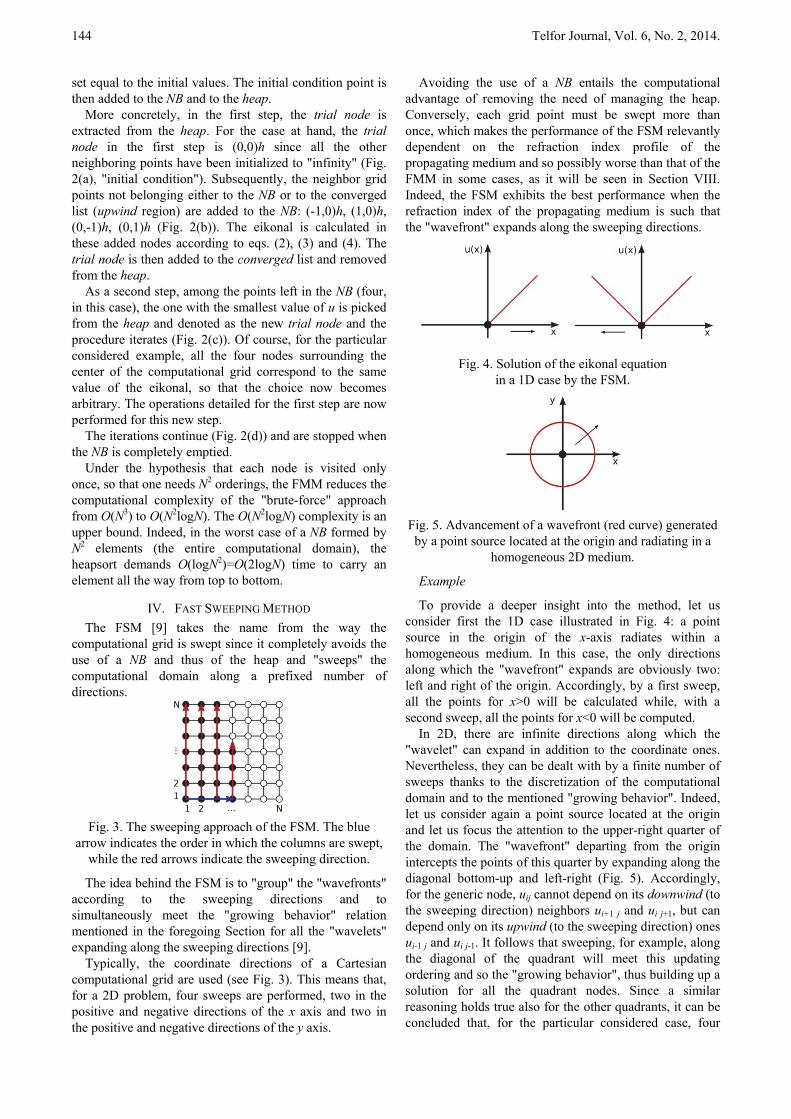
Avoiding the use of a NB entails the computational advantage of removing the need of managing the heap. Conversely, each grid point must be swept more than once, which makes the performance of the FSM relevantly dependent on the refraction index profile of the propagating medium and so possibly worse than that of the FMM in some cases, as it will be seen in Section VIII. Indeed, the FSM exhibits the best performance when the refraction index of the propagating medium is such that the "wavefront" expands along the sweeping directions.

Fig. 4. Solution of the eikonal equation

in a 1D case by the FSM.

Fig. 5. Advancement of a wavefront (red curve) generated by a point source located at the origin and radiating in a

homogeneous 2D medium.

Example

To provide a deeper insight into the method, let us consider first the 1D case illustrated in Fig. 4: a point source in the origin of the x-axis radiates within a homogeneous medium. In this case, the only directions along which the "wavefront" expands are obviously two: left and right of the origin. Accordingly, by a first sweep, all the points for x>0 will be calculated while, with a second sweep, all the points for x<0 will be computed.

In 2D, there are infinite directions along which the "wavelet" can expand in addition to the coordinate ones. Nevertheless, they can be dealt with by a finite number of sweeps thanks to the discretization of the computational domain and to the mentioned "growing behavior". Indeed, let us consider again a point source located at the origin and let us focus the attention to the upper-right quarter of the domain. The "wavefront" departing from the origin intercepts the points of this quarter by expanding along the diagonal bottom-up and left-right (Fig. 5). Accordingly, for the generic node, uij cannot depend on its downwind (to the sweeping direction) neighbors ui+1 j and ui j+1, but can depend only on its upwind (to the sweeping direction) ones ui-1 j and ui j-1. It follows that sweeping, for example, along the diagonal of the quadrant will meet this updating ordering and so the "growing behavior", thus building up a solution for all the quadrant nodes. Since a similar reasoning holds true also for the other quadrants, it can be concluded that, for the particular considered case, four

Capozzoli et al.: A Comparison of Methods for the Solution of the Eikonal Equation 145

sweeping directions will be enough to construct the solution in the whole computational domain. This reasoning can be extended to the 3D case. In general, for an n dimensional problem, 2n sweeping directions are needed to construct the solution.

However, it should be noticed that, for an arbitrary profile of the refraction index, the wavefront will be represented by an arbitrary curve, so that the four directions must be swept more than once to obtain the solution.

V. FAST ITERATIVE METHOD

The FIM conjugates the advantages of the approach in [6] with those of the FMM.

The "brute-force" method in [6] simultaneously updates all the grid nodes until the algorithm convergence is not reached. It is extremely simple to be implemented and does not exploit any ordering or selection, inspired by the "growing behavior", when updating the nodes, thus fitting the SIMD programming model.

As mentioned, the FMM selectively updates the grid nodes by the NB with the aid of a heap structure.

The main idea of the FIM is to selectively update the nodes without maintaining computationally expensive data structures. The FIM has been indeed expressly devised for GPU computing. It is based on three key points:

1. The algorithm must not use any particular order to scan the grid nodes;

2. The algorithm must enable the simultaneous update of grid nodes;

3. The algorithm must not use any heterogeneous data structure to be ordered for storing the active nodes.

The first point is required to guarantee coalesced accesses to the global memory while it should be noticed that the node update scheme of the FMM based on the "growing behavior" would lead to an irregular data access pattern.

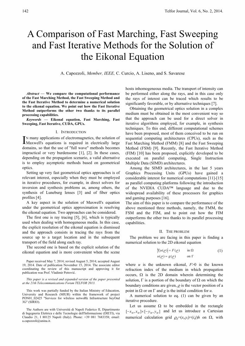
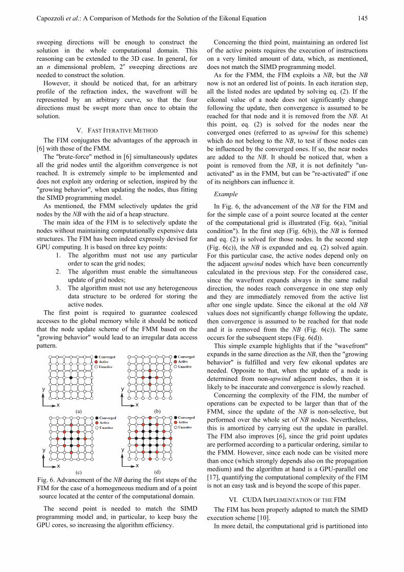
(a) (b)

(c) (d)

Fig. 6. Advancement of the NB during the first steps of the FIM for the case of a homogeneous medium and of a point source located at the center of the computational domain.

The second point is needed to match the SIMD programming model and, in particular, to keep busy the GPU cores, so increasing the algorithm efficiency.

Concerning the third point, maintaining an ordered list of the active points requires the execution of instructions on a very limited amount of data, which, as mentioned, does not match the SIMD programming model.

As for the FMM, the FIM exploits a NB, but the NB now is not an ordered list of points. In each iteration step, all the listed nodes are updated by solving eq. (2). If the eikonal value of a node does not significantly change following the update, then convergence is assumed to be reached for that node and it is removed from the NB. At this point, eq. (2) is solved for the nodes near the converged ones (referred to as upwind for this scheme) which do not belong to the NB, to test if those nodes can be influenced by the converged ones. If so, the near nodes are added to the NB. It should be noticed that, when a point is removed from the NB, it is not definitely "un-activated" as in the FMM, but can be "re-activated" if one of its neighbors can influence it.

Example

In Fig. 6, the advancement of the NB for the FIM and for the simple case of a point source located at the center of the computational grid is illustrated (Fig. 6(a), "initial condition"). In the first step (Fig. 6(b)), the NB is formed and eq. (2) is solved for those nodes. In the second step (Fig. 6(c)), the NB is expanded and eq. (2) solved again. For this particular case, the active nodes depend only on the adjacent upwind nodes which have been concurrently calculated in the previous step. For the considered case, since the wavefront expands always in the same radial direction, the nodes reach convergence in one step only and they are immediately removed from the active list after one single update. Since the eikonal at the old NB values does not significantly change following the update, then convergence is assumed to be reached for that node and it is removed from the NB (Fig. 6(c)). The same occurs for the subsequent steps (Fig. 6(d)).

This simple example highlights that if the "wavefront" expands in the same direction as the NB, then the "growing behavior" is fulfilled and very few eikonal updates are needed. Opposite to that, when the update of a node is determined from non-upwind adjacent nodes, then it is likely to be inaccurate and convergence is slowly reached.

Concerning the complexity of the FIM, the number of operations can be expected to be larger than that of the FMM, since the update of the NB is non-selective, but performed over the whole set of NB nodes. Nevertheless, this is amortized by carrying out the update in parallel. The FIM also improves [6], since the grid point updates are performed according to a particular ordering, similar to the FMM. However, since each node can be visited more than once (which strongly depends also on the propagation medium) and the algorithm at hand is a GPU-parallel one [17], quantifying the computational complexity of the FIM is not an easy task and is beyond the scope of this paper.

VI. CUDA IMPLEMENTATION OF THE FIM

The FIM has been properly adapted to match the SIMD execution scheme [10].

In more detail, the computational grid is partitioned into

146 Telfor Journal, Vol. 6, No. 2, 2014.

a certain number of blocks, each containing a set of nodes and each block is dealt with as it were a node of the above described FMM. The active list now stores the active blocks instead of the active nodes as before so that all the nodes in each block can be simultaneously updated to match the SIMD scheme. Such an update can be performed by a single CUDA kernel launch for which the thread blocks correspond to the node blocks.

After the eikonal values of the generic block have been updated, the block is marked as converged only if all of its nodes have reached convergence. Testing whether all nodes in a block have converged is implemented as a reduction operation.

It should be noticed that the overhead of launching a kernel, and in particular the above mentioned block update kernel, can severely impact the performance of a CUDA application if the kernel is invoked many times. To reduce the impact of this overhead, one possibility is trying to reducing the total number of kernel calls. Since in this scheme a kernel update is invoked for each iteration step, it becomes then crucial to reduce the overall number of iterations. This is obtained by invoking, in each iteration step, a kernel block update also for the blocks near the converged ones.

VII. ALGORITHMS CONVERGENCE

When the NB is completely emptied, the FMM converges.

The FSM and the FIM update the eikonal at a node only if the new value is smaller than the previous one. Accordingly, the numerical solution )(k

iju is a non-

increasing function of k so that

jiuu kij

kij , )1()( (5)

and thus the sequences are converging. In order to show that the solution found by those

algorithms coincides with the solution of the eikonal equation, let us define, according to eq. (2), the quantity

)(kijG as

222)(min

)(2)(min

)()( ])[(])[( hFuuuuG ijk

yk

ijk

xk

ijk

ij

(6)

In [18], it is shown that )(kijG is bounded by (k) defined

as

)(max )()1()( kij

kij

ij

k uu (7)

Thanks to the convergence of )(kiju , we have that

0lim )(

k

k (8)

so that )(k

ijG tends to zero for k.

VIII. RESULTS

In this Section, we compare the computational efficiency of the FMM, the FSM and the FIM on two test cases involving the propagation within a simple

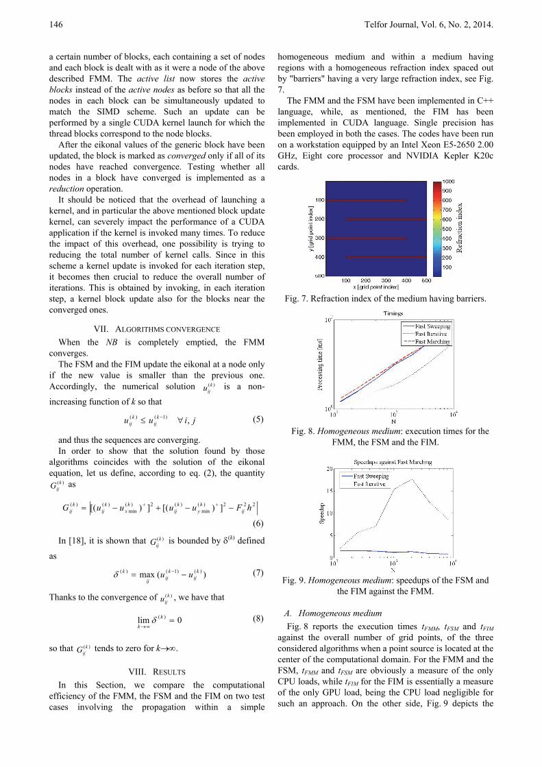
homogeneous medium and within a medium having regions with a homogeneous refraction index spaced out by "barriers" having a very large refraction index, see Fig. 7.

The FMM and the FSM have been implemented in C++ language, while, as mentioned, the FIM has been implemented in CUDA language. Single precision has been employed in both the cases. The codes have been run on a workstation equipped by an Intel Xeon E5-2650 2.00 GHz, Eight core processor and NVIDIA Kepler K20c cards.

Fig. 7. Refraction index of the medium having barriers.

Fig. 8. Homogeneous medium: execution times for the

FMM, the FSM and the FIM.

Fig. 9. Homogeneous medium: speedups of the FSM and

the FIM against the FMM.

A. Homogeneous medium

Fig. 8 reports the execution times tFMM, tFSM and tFIM against the overall number of grid points, of the three considered algorithms when a point source is located at the center of the computational domain. For the FMM and the FSM, tFMM and tFSM are obviously a measure of the only CPU loads, while tFIM for the FIM is essentially a measure of the only GPU load, being the CPU load negligible for such an approach. On the other side, Fig. 9 depicts the

Capozzoli et al.: A Comparison of Methods for the Solution of the Eikonal Equation 147

(adimensional) speedups of the FSM and the FIM against the FMM expressed as tFMM/tFSM and tFMM/tFIM, respectively. For the sake of simplicity, the free space refraction index has been considered. As it can be seen, the CUDA-implemented FIM is significantly faster than the compared approaches, while the FSM results have a better performance than the FMM.

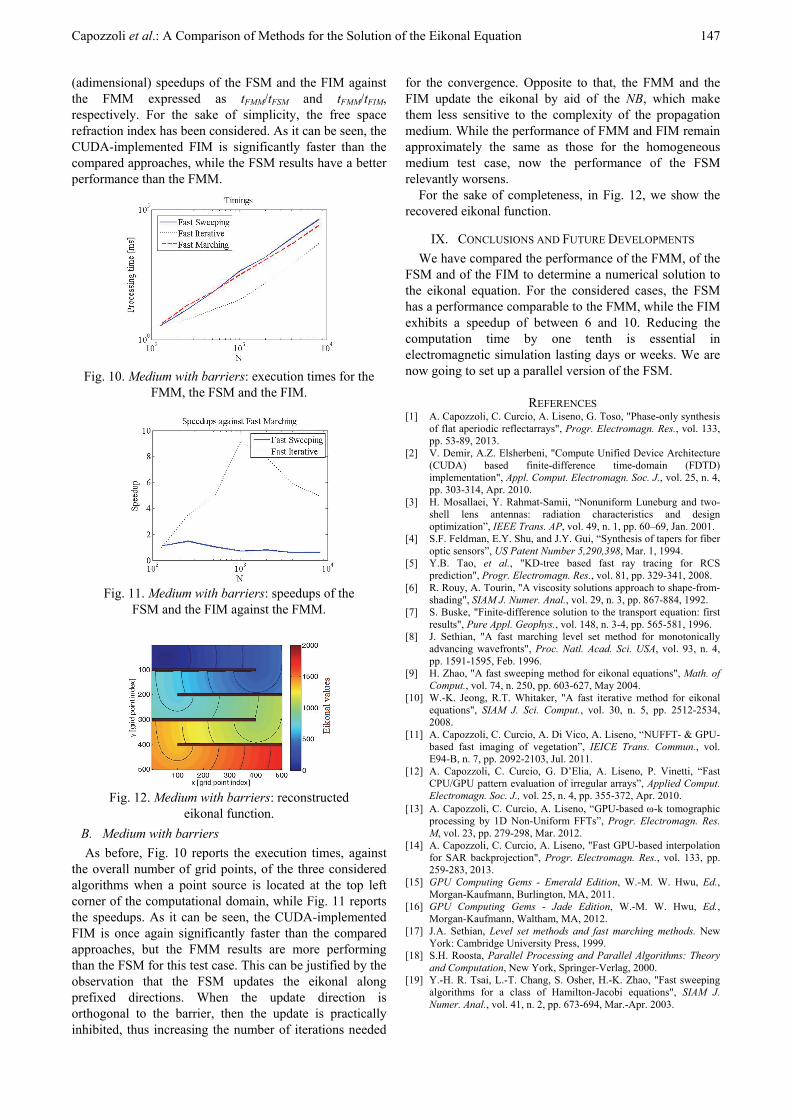
Fig. 10. Medium with barriers: execution times for the

FMM, the FSM and the FIM.

Fig. 11. Medium with barriers: speedups of the

FSM and the FIM against the FMM.

Fig. 12. Medium with barriers: reconstructed

eikonal function.

B. Medium with barriers

As before, Fig. 10 reports the execution times, against the overall number of grid points, of the three considered algorithms when a point source is located at the top left corner of the computational domain, while Fig. 11 reports the speedups. As it can be seen, the CUDA-implemented FIM is once again significantly faster than the compared approaches, but the FMM results are more performing than the FSM for this test case. This can be justified by the observation that the FSM updates the eikonal along prefixed directions. When the update direction is orthogonal to the barrier, then the update is practically inhibited, thus increasing the number of iterations needed

for the convergence. Opposite to that, the FMM and the FIM update the eikonal by aid of the NB, which make them less sensitive to the complexity of the propagation medium. While the performance of FMM and FIM remain approximately the same as those for the homogeneous medium test case, now the performance of the FSM relevantly worsens.

For the sake of completeness, in Fig. 12, we show the recovered eikonal function.

IX. CONCLUSIONS AND FUTURE DEVELOPMENTS

We have compared the performance of the FMM, of the FSM and of the FIM to determine a numerical solution to the eikonal equation. For the considered cases, the FSM has a performance comparable to the FMM, while the FIM exhibits a speedup of between 6 and 10. Reducing the computation time by one tenth is essential in electromagnetic simulation lasting days or weeks. We are now going to set up a parallel version of the FSM.

REFERENCES [1] A. Capozzoli, C. Curcio, A. Liseno, G. Toso, "Phase-only synthesis

of flat aperiodic reflectarrays", Progr. Electromagn. Res., vol. 133, pp. 53-89, 2013.

[2] V. Demir, A.Z. Elsherbeni, "Compute Unified Device Architecture (CUDA) based finite-difference time-domain (FDTD) implementation", Appl. Comput. Electromagn. Soc. J., vol. 25, n. 4, pp. 303-314, Apr. 2010.

[3] H. Mosallaei, Y. Rahmat-Samii, “Nonuniform Luneburg and two-shell lens antennas: radiation characteristics and design optimization”, IEEE Trans. AP, vol. 49, n. 1, pp. 60–69, Jan. 2001.

[4] S.F. Feldman, E.Y. Shu, and J.Y. Gui, “Synthesis of tapers for fiber optic sensors”, US Patent Number 5,290,398, Mar. 1, 1994.

[5] Y.B. Tao, et al., "KD-tree based fast ray tracing for RCS prediction", Progr. Electromagn. Res., vol. 81, pp. 329-341, 2008.

[6] R. Rouy, A. Tourin, "A viscosity solutions approach to shape-from-shading", SIAM J. Numer. Anal., vol. 29, n. 3, pp. 867-884, 1992.

[7] S. Buske, "Finite-difference solution to the transport equation: first results", Pure Appl. Geophys., vol. 148, n. 3-4, pp. 565-581, 1996.

[8] J. Sethian, "A fast marching level set method for monotonically advancing wavefronts", Proc. Natl. Acad. Sci. USA, vol. 93, n. 4, pp. 1591-1595, Feb. 1996.

[9] H. Zhao, "A fast sweeping method for eikonal equations", Math. of Comput., vol. 74, n. 250, pp. 603-627, May 2004.

[10] W.-K. Jeong, R.T. Whitaker, "A fast iterative method for eikonal equations", SIAM J. Sci. Comput., vol. 30, n. 5, pp. 2512-2534, 2008.

[11] A. Capozzoli, C. Curcio, A. Di Vico, A. Liseno, “NUFFT- & GPU-based fast imaging of vegetation”, IEICE Trans. Commun., vol. E94-B, n. 7, pp. 2092-2103, Jul. 2011.

[12] A. Capozzoli, C. Curcio, G. D’Elia, A. Liseno, P. Vinetti, “Fast CPU/GPU pattern evaluation of irregular arrays”, Applied Comput. Electromagn. Soc. J., vol. 25, n. 4, pp. 355-372, Apr. 2010.

[13] A. Capozzoli, C. Curcio, A. Liseno, “GPU-based -k tomographic processing by 1D Non-Uniform FFTs”, Progr. Electromagn. Res. M, vol. 23, pp. 279-298, Mar. 2012.

[14] A. Capozzoli, C. Curcio, A. Liseno, "Fast GPU-based interpolation for SAR backprojection", Progr. Electromagn. Res., vol. 133, pp. 259-283, 2013.

[15] GPU Computing Gems - Emerald Edition, W.-M. W. Hwu, Ed., Morgan-Kaufmann, Burlington, MA, 2011.

[16] GPU Computing Gems - Jade Edition, W.-M. W. Hwu, Ed., Morgan-Kaufmann, Waltham, MA, 2012.

[17] J.A. Sethian, Level set methods and fast marching methods. New York: Cambridge University Press, 1999.

[18] S.H. Roosta, Parallel Processing and Parallel Algorithms: Theory and Computation, New York, Springer-Verlag, 2000.

[19] Y.-H. R. Tsai, L.-T. Chang, S. Osher, H.-K. Zhao, "Fast sweeping algorithms for a class of Hamilton-Jacobi equations", SIAM J. Numer. Anal., vol. 41, n. 2, pp. 673-694, Mar.-Apr. 2003.