A Comparison of Image Segmentation Algorithms · A Comparison of Image Segmentation Algorithms ... A system designer now has an array of available algorithm choices, how- ... mentation

A Comparison of Image SegmentationAlgorithms

Caroline Pantofaru Martial Hebert

CMU-RI-TR-05-40

September 1, 2005

The Robotics InstituteCarnegie Mellon University

Pittsburgh, Pennsylvania 15213

c© Carnegie Mellon University

Abstract

Unsupervised image segmentation algorithms have matured to the point where theygenerate reasonable segmentations, and thus can begin to be incorporated into largersystems. A system designer now has an array of available algorithm choices, how-ever, few objective numerical evaluations exist of these segmentation algorithms. As afirst step towards filling this gap, this paper presents an evaluation of two popular seg-mentation algorithms, the mean shift-based segmentation algorithm and a graph-basedsegmentation scheme. We also consider a hybrid method which combines the othertwo methods. This quantitative evaluation is made possible by the recently proposedmeasure of segmentation correctness, the Normalized Probabilistic Rand (NPR) index,which allows a principled comparison between segmentations created by different al-gorithms, as well as segmentations on different images.

For each algorithm, we consider its correctness as measured by the NPR index,as well as its stability with respect to changes in parameter settings and with respectto different images. An algorithm which produces correct segmentation results witha wide array of parameters on any one image, as well as correct segmentation resultson multiple images with the same parameters, will be a useful, predictable and easilyadjustable preprocessing step in a larger system.

Our results are presented on the Berkeley image segmentation database, whichcontains 300 natural images along with several ground truth hand segmentations foreach image. As opposed to previous results presented on this database, the algorithmswe compare all use the same image features (position and colour) for segmentation,thereby making their outputs directly comparable.

I

Contents

1 Introduction 1

2 Previous Work 2

3 The Segmentation Algorithms 23.1 Mean Shift Segmentation. . . . . . . . . . . . . . . . . . . . . . . . 3

3.1.1 Filtering. . . . . . . . . . . . . . . . . . . . . . . . . . . . . 33.1.2 Clustering. . . . . . . . . . . . . . . . . . . . . . . . . . . . 43.1.3 Discussion . . . . . . . . . . . . . . . . . . . . . . . . . . . 4

3.2 Efficient Graph-based Segmentation. . . . . . . . . . . . . . . . . . 53.3 Hybrid Segmentation Algorithm. . . . . . . . . . . . . . . . . . . . 6

4 Evaluation Methodology 74.1 Normalized Probabilistic Rand (NPR) Index. . . . . . . . . . . . . . 74.2 Comparisons . . . . . . . . . . . . . . . . . . . . . . . . . . . . . . 10

5 Experiments 105.1 Maximum performance. . . . . . . . . . . . . . . . . . . . . . . . . 115.2 Average performance per image. . . . . . . . . . . . . . . . . . . . 12

5.2.1 Average performance over all parameter combinations. . . . 125.2.2 Average performance over different values of the colour band-

width hr . . . . . . . . . . . . . . . . . . . . . . . . . . . . 145.2.3 Average performance over different values ofk . . . . . . . . 14

5.3 Average performance per parameter choice. . . . . . . . . . . . . . 195.3.1 Average performance over all images for different values ofhr 195.3.2 Average performance over all images for different values ofk 19

6 Summary and Conclusions 24

III

1 Introduction

Unsupervised image segmentation algorithms have matured to the point that they pro-vide segmentations which agree to a large extent with human intuition. The time hasarrived for these segmentations to play a larger role in object recognition. It is clearthat unsupervised segmentation can be used to help cue and refine various recognitionalgorithms. However, one of the stumbling blocks that remains is that it is unknownexactly how well these segmentation algorithms perform from an objective standpoint.Most presentations of segmentation algorithms contain superficial evaluations whichmerely display images of the segmentation results and appeal to the reader’s intuitionfor evaluation. There is a consistent lack of numerical results, thus it is difficult to knowwhich segmentation algorithms present useful results and in which situations they doso. Appealing to human intuition is convenient, however if the algorithm is going to beused in an automated system then objective results on large datasets are to be desired.

In this paper we present the results of an objective evaluation of two popular seg-mentation techniques: mean shift segmentation [1], and the efficient graph-based seg-mentation algorithm presented in [4]. As well, we look at a hybrid variant that com-bines these algorithms. For each of these algorithms, we examine three characteristics:

1. Correctness: the ability to produce segmentations which agree with human intu-ition. That is, segmentations which correctly identify structures in the image atneither too fine nor too coarse a level of detail.

2. Stability with respect to parameter choice: the ability to produce segmentationsof consistent correctness for a range of parameter choices.

3. Stability with respect to image choice: the ability to produce segmentations ofconsistent correctness using the same parameter choice on a wide range of dif-ferent images.

If a segmentation scheme satisfies these three characteristics, then it will give usefuland predictable results which can be reliably incorporated into a larger system.

The measure we use to evaluate these algorithms is the recently proposed Normal-ized Probabilistic Rand (NPR) index [6]. We chose to use this measure as it allows aprincipled comparison between segmentation results on different images, with differingnumbers of regions, and generated by different algorithms with different parameters.Also, the NPR index of one segmentation is meaningful as an absolute score, not just incomparison with that of another segmentation. These characteristics are all necessaryfor the comparison we wish to perform.

Our dataset for this evaluation is the Berkeley Segmentation Database [5], whichcontains 300 natural images with multiple ground truth hand segmentations of each im-age. To ensure a valid comparison between algorithms, we compute the same features(pixel location and colour) for every image and every segmentation algorithm.

This paper is organized as follows. We begin by presenting some previous work oncomparing segmentations and clusterings. Then, we present each of the segmentationalgorithms and the hybrid variant we considered. Next, we describe the NPR index andpresent the reasons for using this measure, followed by a description of our comparisonmethodology. Finally, we present our results.

1

2 Previous Work

There have been previous attempts at numerical image segmentation method compar-isons, although the number is small. Here we describe some examples and summarizehow our work differs.

A comparison of spectral clustering methods is given in [8]. The authors attemptedto compare variants of four popular spectral clustering algorithms: normalized cuts byShi and Malik [13], a variant by Kannan, Vempala and Vetta [9], the algorithm by Ng,Jordan and Weiss [11], and the Multicut algorithm by Meila and Shi [10], as well asSingle and Ward linkage as a base for comparison. They also combined different partsof different algorithms to create new ones. The measure of correctness used was theVariation of Information introduced in [12], which considers the conditional entropiesbetween the labels in two segmentations. The results of this comparison were largelyunexciting, with all of the algorithms and variants performing well on ‘easy’ data, andall performing roughly equally badly on ‘hard’ data.

Another attempt at segmentation algorithm comparison is presented on the Berke-ley database and segmentation comparison website [5]. Here a large set of imagesare made available for segmentation evaluation, and a framework is set up to facilitatecomparison. Comparisons currently exist between using cues of brightness, texture,and/or edges for segmentation. However, there are no current examples of comparisonsbetween actual algorithms which use the same features. The measure used for segmen-tation correctness is a precision-recall curve based on the correctness of each regionboundary pixel. Different boundary thresholds are used to obtain different points onthe curve. The reported statistic is the F-measure, the harmonic mean of the precisionand recall. This measure has the downside of considering only region boundaries in-stead of the regions themselves. Since region difference is a quadratic measure whereasboundary difference is a linear measure, small boundary imperfections will affect themeasure more than they necessarily should.

Our current work is the first which presents a segmentation algorithm comparisonwithin a framework which is independent of the features used, which compares eachof the three traits of correctness and stability with respect to parameters and images,and which uses a measure of correctness which can compare all of the necessary seg-mentations in a principled and valid manner. In addition, we consider two popular butpreviously unevaluated algorithms.

3 The Segmentation Algorithms

As mentioned, we will compare three different segmentation techniques, the meanshift-based segmentation algorithm [1], an efficient graph-based segmentation algo-rithm [4], and a hybrid of the two. We have chosen to look at mean shift-based segmen-tation as it is generally effective and has become widely-used in the vision community.The efficient graph-based segmentation algorithm was chosen as an interesting com-parison to the mean shift in that its general approach is similar, however it excludes themean shift filtering step itself, thus partially addressing the question of whether the fil-tering step is useful. The combination of the two algorithms is shown as an attempt toimprove the performance and stability of either one alone. In this section we describeeach algorithm and further discuss how they differ from one another.

2

3.1 Mean Shift Segmentation

The mean shift based segmentation technique was introduced in [1] and has becomewidely-used in the vision community. It is one of many techniques under the headingof “feature space analysis”. The mean shift technique is comprised of two basic steps:a mean shift filtering of the original image data (in feature space), and a subsequentclustering of the filtered data points. Below we will briefly describe each of these stepsand then discuss some of the strengths and weaknesses of this method.

3.1.1 Filtering

The filtering step of the mean shift segmentation algorithm consists of analyzing theprobability density function underlying the image data in feature space. Consider thefeature space consisting of the original image data represented as the(x, y) locationof each pixel, plus its colour in L*u*v* space(L∗, u∗, v∗). The modes of the pdfunderlying the data in this space will correspond to the locations with highest datadensity. In terms of a segmentation, it is intuitive that the data points close to thesehigh density points (modes) should be clustered together. Note that these modes arealso far less sensitive to outliers than the means of, say, a mixture of Gaussians wouldbe.

The mean shift filtering step consists of finding the modes of the underlying pdf andassociating with them any points in their basin of attraction. Unlike earlier techniques,the mean shift is a non-parametric technique and hence we will need to estimate thegradient of the pdf,f(x), in an iterative manner using kernel density estimation to findthe modes. For a data pointx in feature space, the density gradient is estimated asbeing proportional to the mean shift vector:

∇f(x) ∝∑n

i=1 xig(‖x−xi

h ‖)∑n

i=1 g(‖x−xi

h ‖) − x (1)

wherexi are the data points,x is a point in the feature space,n is the number ofdatapoints (pixels in the image), andg is the profile of the symmetric kernelG. We usethe simple case whereG is the uniform kernel with radius vectorh. Thus the aboveequation simplifies to:

∇f(x) ∝

1|Sx,hs,hr |

∑xi∈Sx,hs,hr

xi

− x (2)

whereSx,hs,hrrepresents the sphere in feature space centered atx and having spatial

radiushs and colour (range) radiushr, and thexi represent the data points within thatsphere.

For every data point (pixel in the original image)x we can iteratively compute thegradient estimate in Eqn.2 and movex in that direction, until the gradient is below athreshold. Thus we have found the points where∇f(x′) = 0, the modes of the densityestimate. We can then replace the pointx with x′, the mode with which it is associated.

Finding the mode associated with each data point helps to smooth the image whilepreserving discontinuities. Intuitively, if two pointsxi andxj are far from each otherin feature space, thenxi 6∈ Sxj ,hs,hr

and hencexj doesn’t contribute to the mean shiftvector gradient estimate and the trajectory ofxi will move it away fromxj . Hence,

3

(a) (b) (c) (d)

(e) (f) (g)

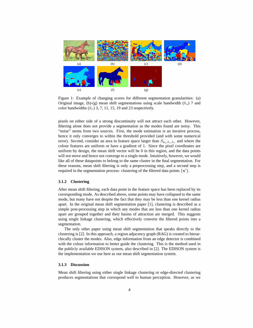
Figure 1: Example of changing scores for different segmentation granularities: (a)Original image, (b)-(g) mean shift segmentations using scale bandwidth (hs) 7 andcolor bandwidths (hr) 3, 7, 11, 15, 19 and 23 respectively.

pixels on either side of a strong discontinuity will not attract each other. However,filtering alone does not provide a segmentation as the modes found are noisy. This“noise” stems from two sources. First, the mode estimation is an iterative process,hence it only converges to within the threshold provided (and with some numericalerror). Second, consider an area in feature space larger thanSxj ,hs,hr and where thecolour features are uniform or have a gradient of 1. Since the pixel coordinates areuniform by design, the mean shift vector will be 0 in this region, and the data pointswill not move and hence not converge to a single mode. Intuitively, however, we wouldlike all of these datapoints to belong to the same cluster in the final segmentation. Forthese reasons, mean shift filtering is only a preprocessing step, and a second step isrequired in the segmentation process: clustering of the filtered data points{x′}.

3.1.2 Clustering

After mean shift filtering, each data point in the feature space has been replaced by itscorresponding mode. As described above, some points may have collapsed to the samemode, but many have not despite the fact that they may be less than one kernel radiusapart. In the original mean shift segmentation paper [1], clustering is described as asimple post-processing step in which any modes that are less than one kernel radiusapart are grouped together and their basins of attraction are merged. This suggestsusing single linkage clustering, which effectively converts the filtered points into asegmentation.

The only other paper using mean shift segmentation that speaks directly to theclustering is [2]. In this approach, a region adjacency graph (RAG) is created to hierar-chically cluster the modes. Also, edge information from an edge detector is combinedwith the colour information to better guide the clustering. This is the method used inthe publicly available EDISON system, also described in [2]. The EDISON system isthe implementation we use here as our mean shift segmentation system.

3.1.3 Discussion

Mean shift filtering using either single linkage clustering or edge-directed clusteringproduces segmentations that correspond well to human perception. However, as we

4

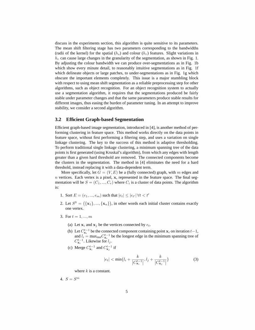
discuss in the experiments section, this algorithm is quite sensitive to its parameters.The mean shift filtering stage has two parameters corresponding to the bandwidths(radii of the kernel) for the spatial (hs) and colour (hr) features. Slight variations inhr can cause large changes in the granularity of the segmentation, as shown in Fig.1.By adjusting the colour bandwidth we can produce over-segmentations as in Fig.1bwhich show every minute detail, to reasonably intuitive segmentations as in Fig.1fwhich delineate objects or large patches, to under-segmentations as in Fig.1g whichobscure the important elements completely. This issue is a major stumbling blockwith respect to using mean shift segmentation as a reliable preprocessing step for otheralgorithms, such as object recognition. For an object recognition system to actuallyuse a segmentation algorithm, it requires that the segmentations produced be fairlystable under parameter changes and that the same parameters produce stable results fordifferent images, thus easing the burden of parameter tuning. In an attempt to improvestability, we consider a second algorithm.

3.2 Efficient Graph-based Segmentation

Efficient graph-based image segmentation, introduced in [4], is another method of per-forming clustering in feature space. This method works directly on the data points infeature space, without first performing a filtering step, and uses a variation on singlelinkage clustering. The key to the success of this method is adaptive thresholding.To perform traditional single linkage clustering, a minimum spanning tree of the datapoints is first generated (using Kruskal’s algorithm), from which any edges with lengthgreater than a given hard threshold are removed. The connected components becomethe clusters in the segmentation. The method in [4] eliminates the need for a hardthreshold, instead replacing it with a data-dependent term.

More specifically, letG = (V,E) be a (fully connected) graph, withm edges andn vertices. Each vertex is a pixel,x, represented in the feature space. The final seg-mentation will beS = (C1, ..., Cr) whereCi is a cluster of data points. The algorithmis:

1. SortE = (e1, ..., em) such that|et| ≤ |et′ | ∀t < t′

2. Let S0 =({x1}, ..., {xn}

), in other words each initial cluster contains exactly

one vertex.

3. For t = 1, ...,m

(a) Let xi andxj be the vertices connected byet.

(b) LetCt−1xi

be the connected component containing pointxi on iterationt−1,andli = maxmstC

t−1xi

be the longest edge in the minimum spanning tree ofCt−1

xi. Likewise forlj .

(c) MergeCt−1xi

andCt−1xj

if

|et| < min{li +k∣∣Ct−1xi

∣∣ , lj +k∣∣Ct−1xj

∣∣} (3)

wherek is a constant.

4. S = Sm

5

(a) (b) (c) (d)

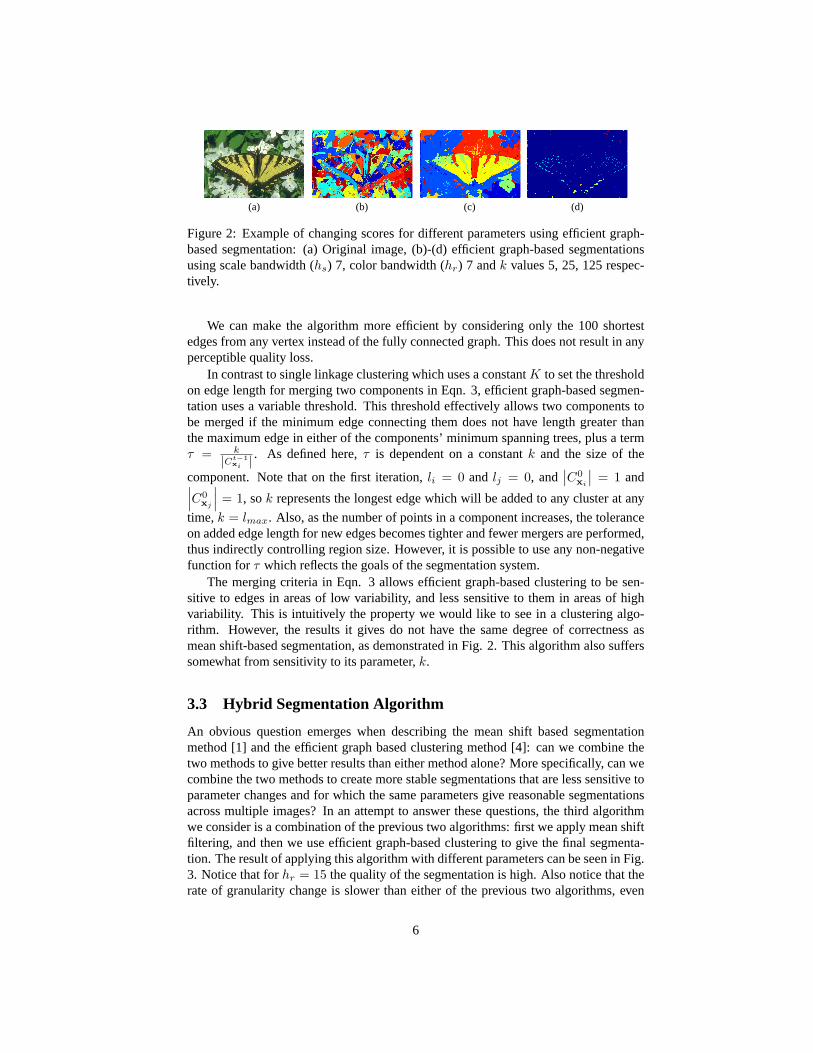
Figure 2: Example of changing scores for different parameters using efficient graph-based segmentation: (a) Original image, (b)-(d) efficient graph-based segmentationsusing scale bandwidth (hs) 7, color bandwidth (hr) 7 andk values 5, 25, 125 respec-tively.

We can make the algorithm more efficient by considering only the 100 shortestedges from any vertex instead of the fully connected graph. This does not result in anyperceptible quality loss.

In contrast to single linkage clustering which uses a constantK to set the thresholdon edge length for merging two components in Eqn.3, efficient graph-based segmen-tation uses a variable threshold. This threshold effectively allows two components tobe merged if the minimum edge connecting them does not have length greater thanthe maximum edge in either of the components’ minimum spanning trees, plus a termτ = k

|Ct−1xi | . As defined here,τ is dependent on a constantk and the size of the

component. Note that on the first iteration,li = 0 and lj = 0, and∣∣C0

xi

∣∣ = 1 and∣∣∣C0xj

∣∣∣ = 1, sok represents the longest edge which will be added to any cluster at any

time,k = lmax. Also, as the number of points in a component increases, the toleranceon added edge length for new edges becomes tighter and fewer mergers are performed,thus indirectly controlling region size. However, it is possible to use any non-negativefunction forτ which reflects the goals of the segmentation system.

The merging criteria in Eqn.3 allows efficient graph-based clustering to be sen-sitive to edges in areas of low variability, and less sensitive to them in areas of highvariability. This is intuitively the property we would like to see in a clustering algo-rithm. However, the results it gives do not have the same degree of correctness asmean shift-based segmentation, as demonstrated in Fig.2. This algorithm also sufferssomewhat from sensitivity to its parameter,k.

3.3 Hybrid Segmentation Algorithm

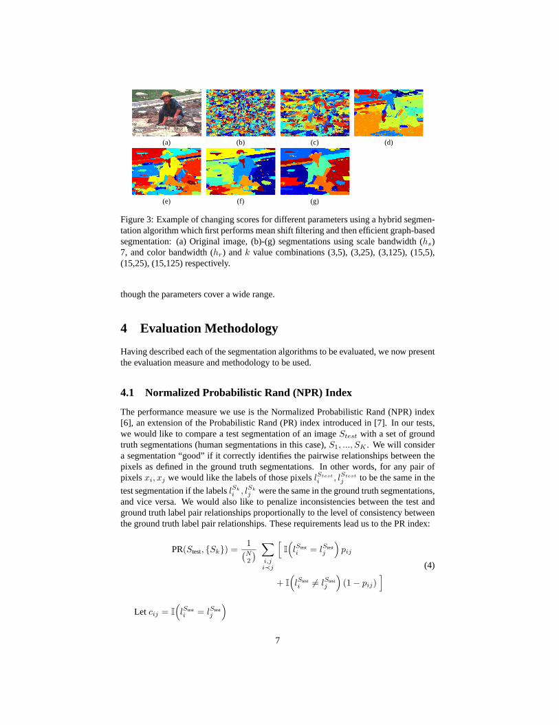
An obvious question emerges when describing the mean shift based segmentationmethod [1] and the efficient graph based clustering method [4]: can we combine thetwo methods to give better results than either method alone? More specifically, can wecombine the two methods to create more stable segmentations that are less sensitive toparameter changes and for which the same parameters give reasonable segmentationsacross multiple images? In an attempt to answer these questions, the third algorithmwe consider is a combination of the previous two algorithms: first we apply mean shiftfiltering, and then we use efficient graph-based clustering to give the final segmenta-tion. The result of applying this algorithm with different parameters can be seen in Fig.3. Notice that forhr = 15 the quality of the segmentation is high. Also notice that therate of granularity change is slower than either of the previous two algorithms, even

6

(a) (b) (c) (d)

(e) (f) (g)

Figure 3: Example of changing scores for different parameters using a hybrid segmen-tation algorithm which first performs mean shift filtering and then efficient graph-basedsegmentation: (a) Original image, (b)-(g) segmentations using scale bandwidth (hs)7, and color bandwidth (hr) andk value combinations (3,5), (3,25), (3,125), (15,5),(15,25), (15,125) respectively.

though the parameters cover a wide range.

4 Evaluation Methodology

Having described each of the segmentation algorithms to be evaluated, we now presentthe evaluation measure and methodology to be used.

4.1 Normalized Probabilistic Rand (NPR) Index

The performance measure we use is the Normalized Probabilistic Rand (NPR) index[6], an extension of the Probabilistic Rand (PR) index introduced in [7]. In our tests,we would like to compare a test segmentation of an imageStest with a set of groundtruth segmentations (human segmentations in this case),S1, ..., SK . We will considera segmentation “good” if it correctly identifies the pairwise relationships between thepixels as defined in the ground truth segmentations. In other words, for any pair ofpixelsxi, xj we would like the labels of those pixelslStest

i , lStestj to be the same in the

test segmentation if the labelslSki , lSk

j were the same in the ground truth segmentations,and vice versa. We would also like to penalize inconsistencies between the test andground truth label pair relationships proportionally to the level of consistency betweenthe ground truth label pair relationships. These requirements lead us to the PR index:

PR(Stest, {Sk}) =1(N2

) ∑i,ji≺j

[I(lStesti = lStest

j

)pij

+ I(lStesti 6= lStest

j

)(1− pij)

] (4)

Let cij = I(lStesti = lStest

j

)7

Then the PR index can be written as:

PR(Stest, {Sk}) =1(N2

) ∑i,ji≺j

[cijpij + (1− cij)(1− pij)] (5)

Where N is the number of pixels, andpij is the ground truth probability that

I(li = lj). In practicepij = 1K

∑I(lSki = lSk

j

), the mean pixel pair relationship

among the ground truth images. The PR index takes a value in the interval[0, 1], anda PR index of 0 or 1 can only be achieved when all of the ground truth segmentationsagree on every pixel pair relationship. A score of 0 indicates that every pixel pair inthe test image has the opposite relationship as every pair in the ground truth segmenta-tions, while a score of 1 indicates that every pixel pair in the test image has the samerelationship as every pair in the ground truth segmentations.

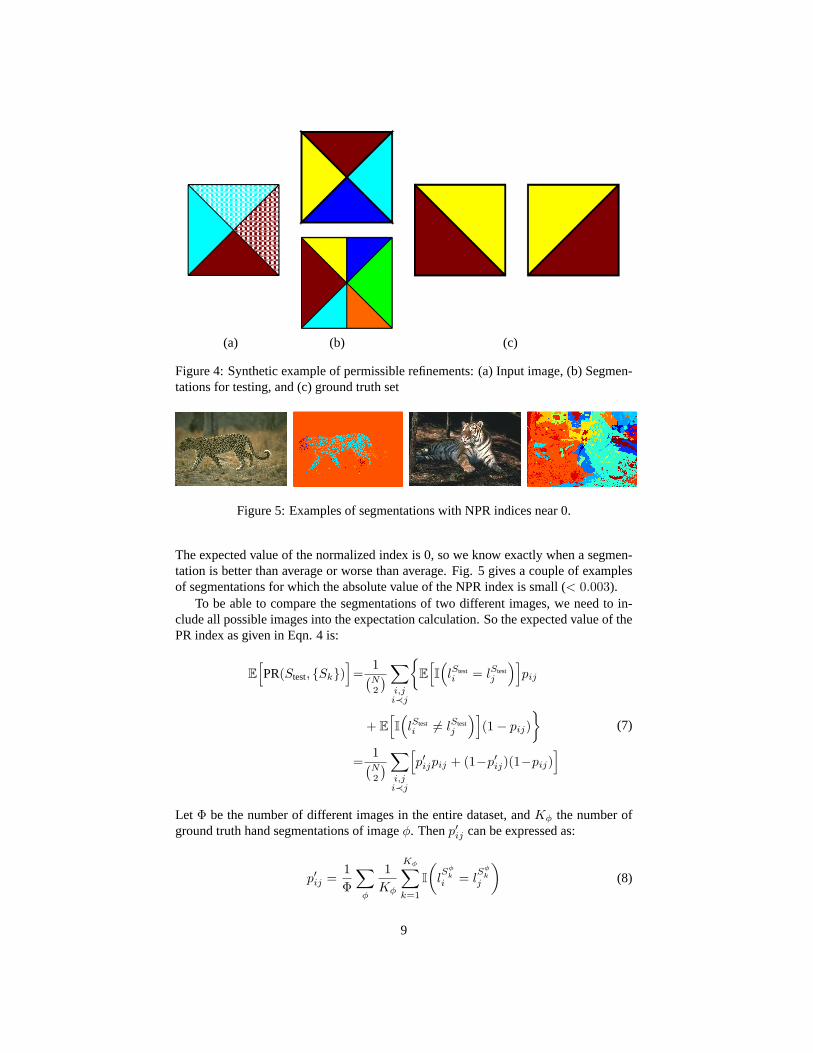
As described in [7], the PR index has the desirable property that it does not allowarbitrary refinements or generalizations of the ground truth segmentations. In otherwords, if two pixels are in the same region in most of the ground truth segmentations,they are penalized for not being in the same region in the test segmentation, and viceversa. Also, the penalization is dependent on the fraction of disagreeing ground truthsegmentations. Thus, there is a smaller penalty for disagreeing with an inherently am-biguous pixel pair than with a pixel pair on which all of the ground truths agree. Anexample of this refinement policy is shown in Fig.4. Fig. 4a shows an image, Fig.4b shows two test segmentations, and Fig.4c shows the ground truth hand segmen-tations for that image. It appears as though the first ground truth labeling is based ontexture, while the second is based on colour. The top test segmentation only has regiondivisions that exist in at least one of the two ground truth images, it has divided theimage based on both colour and texture. The bottom test segmentation, however, hasregion divisions which exist in neither of the ground truth images. Thus, the top testsegmentation will have a higher index than the bottom one.

This refinement policy is attractive for evaluating most segmentation tasks in whichwe would like to avoid arbitrary refining and coarsening of a segmentation. For exam-ple, for an object recognition system, it is important to differentiate between a segmen-tation which gives object-level regions, one which gives part-level regions, and onewhich gives even smaller over-segmented regions. However, if your application is notsensitive to different granularities, a different measure should be used, such as the LCE[14].

The PR index does however have one serious flaw. Note that the PR index is ona scale of 0-1, but there is no expected value for a given segmentation. That is, itis impossible to know if any given score is good or bad. The best we can hope todo is compare it to the score of another segmentation of the same image, but still wedo not know if the difference between the two scores is relevant or not. Also, wecertainly can not compare the score of a segmentation of one image with the score ofa segmentation of another image. All of these issues are resolved with normalizationto produce the Normalized Probabilistic Rand (NPR) index [6]. The NPR index uses atypical normalization scheme: if the baseline index value is the expected value of theindex of any given segmentation of a particular image, then

Normalized index=Index− Expected index

Maximum index− Expected index(6)

8

(a) (b) (c)

Figure 4: Synthetic example of permissible refinements: (a) Input image, (b) Segmen-tations for testing, and (c) ground truth set

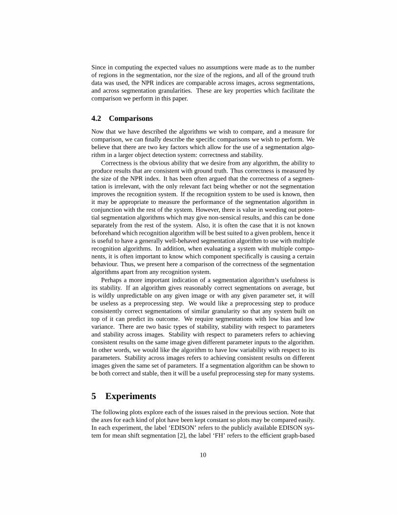
Figure 5: Examples of segmentations with NPR indices near 0.

The expected value of the normalized index is 0, so we know exactly when a segmen-tation is better than average or worse than average. Fig.5 gives a couple of examplesof segmentations for which the absolute value of the NPR index is small (< 0.003).

To be able to compare the segmentations of two different images, we need to in-clude all possible images into the expectation calculation. So the expected value of thePR index as given in Eqn.4 is:

E[PR(Stest, {Sk})

]=

1(N2

) ∑i,ji≺j

{E

[I(lStesti = lStest

j

)]pij

+ E[I(lStesti 6= lStest

j

)](1− pij)

}=

1(N2

) ∑i,ji≺j

[p′ijpij + (1−p′ij)(1−pij)

] (7)

Let Φ be the number of different images in the entire dataset, andKφ the number ofground truth hand segmentations of imageφ. Thenp′ij can be expressed as:

p′ij =1Φ

∑φ

1Kφ

Kφ∑k=1

I(

lSφ

ki = l

Sφk

j

)(8)

9

Since in computing the expected values no assumptions were made as to the numberof regions in the segmentation, nor the size of the regions, and all of the ground truthdata was used, the NPR indices are comparable across images, across segmentations,and across segmentation granularities. These are key properties which facilitate thecomparison we perform in this paper.

4.2 Comparisons

Now that we have described the algorithms we wish to compare, and a measure forcomparison, we can finally describe the specific comparisons we wish to perform. Webelieve that there are two key factors which allow for the use of a segmentation algo-rithm in a larger object detection system: correctness and stability.

Correctness is the obvious ability that we desire from any algorithm, the ability toproduce results that are consistent with ground truth. Thus correctness is measured bythe size of the NPR index. It has been often argued that the correctness of a segmen-tation is irrelevant, with the only relevant fact being whether or not the segmentationimproves the recognition system. If the recognition system to be used is known, thenit may be appropriate to measure the performance of the segmentation algorithm inconjunction with the rest of the system. However, there is value in weeding out poten-tial segmentation algorithms which may give non-sensical results, and this can be doneseparately from the rest of the system. Also, it is often the case that it is not knownbeforehand which recognition algorithm will be best suited to a given problem, hence itis useful to have a generally well-behaved segmentation algorithm to use with multiplerecognition algorithms. In addition, when evaluating a system with multiple compo-nents, it is often important to know which component specifically is causing a certainbehaviour. Thus, we present here a comparison of the correctness of the segmentationalgorithms apart from any recognition system.

Perhaps a more important indication of a segmentation algorithm’s usefulness isits stability. If an algorithm gives reasonably correct segmentations on average, butis wildly unpredictable on any given image or with any given parameter set, it willbe useless as a preprocessing step. We would like a preprocessing step to produceconsistently correct segmentations of similar granularity so that any system built ontop of it can predict its outcome. We require segmentations with low bias and lowvariance. There are two basic types of stability, stability with respect to parametersand stability across images. Stability with respect to parameters refers to achievingconsistent results on the same image given different parameter inputs to the algorithm.In other words, we would like the algorithm to have low variability with respect to itsparameters. Stability across images refers to achieving consistent results on differentimages given the same set of parameters. If a segmentation algorithm can be shown tobe both correct and stable, then it will be a useful preprocessing step for many systems.

5 Experiments

The following plots explore each of the issues raised in the previous section. Note thatthe axes for each kind of plot have been kept constant so plots may be compared easily.In each experiment, the label ‘EDISON’ refers to the publicly available EDISON sys-tem for mean shift segmentation [2], the label ‘FH’ refers to the efficient graph-based

10

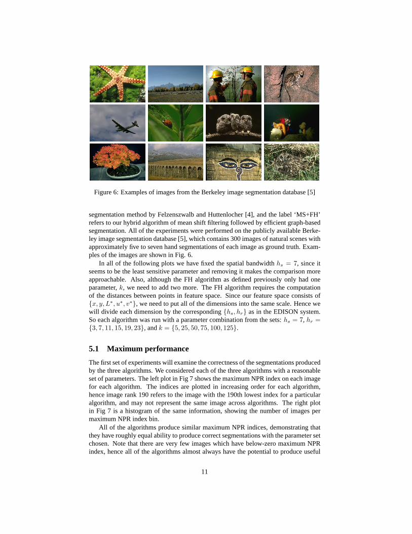
Figure 6: Examples of images from the Berkeley image segmentation database [5]

segmentation method by Felzenszwalb and Huttenlocher [4], and the label ‘MS+FH’refers to our hybrid algorithm of mean shift filtering followed by efficient graph-basedsegmentation. All of the experiments were performed on the publicly available Berke-ley image segmentation database [5], which contains 300 images of natural scenes withapproximately five to seven hand segmentations of each image as ground truth. Exam-ples of the images are shown in Fig.6.

In all of the following plots we have fixed the spatial bandwidthhs = 7, since itseems to be the least sensitive parameter and removing it makes the comparison moreapproachable. Also, although the FH algorithm as defined previously only had oneparameter,k, we need to add two more. The FH algorithm requires the computationof the distances between points in feature space. Since our feature space consists of{x, y, L∗, u∗, v∗}, we need to put all of the dimensions into the same scale. Hence wewill divide each dimension by the corresponding{hs, hr} as in the EDISON system.So each algorithm was run with a parameter combination from the sets:hs = 7, hr ={3, 7, 11, 15, 19, 23}, andk = {5, 25, 50, 75, 100, 125}.

5.1 Maximum performance

The first set of experiments will examine the correctness of the segmentations producedby the three algorithms. We considered each of the three algorithms with a reasonableset of parameters. The left plot in Fig7 shows the maximum NPR index on each imagefor each algorithm. The indices are plotted in increasing order for each algorithm,hence image rank 190 refers to the image with the 190th lowest index for a particularalgorithm, and may not represent the same image across algorithms. The right plotin Fig 7 is a histogram of the same information, showing the number of images permaximum NPR index bin.

All of the algorithms produce similar maximum NPR indices, demonstrating thatthey have roughly equal ability to produce correct segmentations with the parameter setchosen. Note that there are very few images which have below-zero maximum NPRindex, hence all of the algorithms almost always have the potential to produce useful

11

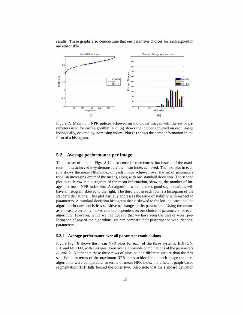
results. These graphs also demonstrate that our parameter choices for each algorithmare reasonable.

50 100 150 200 250−2

−1.5

−1

−0.5

0

0.5

1

Image rank

NP

R in

dex

Max NPR vs image

EDISONFHMS + FH

−1 −0.5 0 0.5 10

10

20

30

40

50

60

70

80

90

100Percent of images per max index

NPR index

Per

cent

of i

mag

es

EDISONFHMS + FH

(a) (b)

Figure 7: Maximum NPR indices achieved on individual images with the set of pa-rameters used for each algorithm. Plot (a) shows the indices achieved on each imageindividually, ordered by increasing index. Plot (b) shows the same information in theform of a histogram.

5.2 Average performance per image

The next set of plots in Figs.8-12 also consider correctness, but instead of the maxi-mum index achieved they demonstrate the mean index achieved. The first plot in eachrow shows the mean NPR index on each image achieved over the set of parametersused (in increasing order of the mean), along with one standard deviation. The secondplot in each row is a histogram of the mean information, showing the number of im-ages per mean NPR index bin. An algorithm which creates good segmentations willhave a histogram skewed to the right. The third plot in each row is a histogram of thestandard deviations. This plot partially addresses the issue of stability with respect toparameters. A standard deviation histogram that is skewed to the left indicates that thealgorithm in question is less sensitive to changes in its parameters. Using the meansas a measure certainly makes us more dependent on our choice of parameters for eachalgorithm. However, while we can not say that we have seen the best or worst per-formance of any of the algorithms, we can compare their performance with identicalparameters.

5.2.1 Average performance over all parameter combinations

Figure Fig. 8 shows the mean NPR plots for each of the three systems, EDISON,FH, and MS+FH, with averages taken over all possible combinations of the parametershr andk. Notice that these three rows of plots paint a different picture than the firstset. While in terms of the maximum NPR index achievable on each image the threealgorithms were comparable, in terms of mean NPR index the efficient graph-basedsegmentation (FH) falls behind the other two. Also note that the standard deviation

12

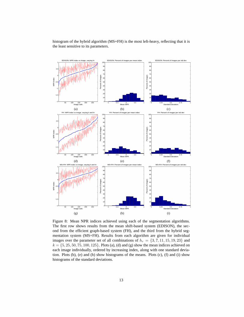
histogram of the hybrid algorithm (MS+FH) is the most left-heavy, reflecting that it isthe least sensitive to its parameters.

50 100 150 200 250−2

−1.5

−1

−0.5

0

0.5

1

Image rank

NP

R in

dex

EDISON: NPR index vs image, varying hr

−1 −0.5 0 0.5 10

10

20

30

40

50

60

70

80

90

100

Mean NPR

Per

cent

of i

mag

es

EDISON: Percent of images per mean index

0 0.25 0.5 0.75 10

10

20

30

40

50

60

70

80

90

100

Standard deviation

Per

cent

of i

mag

es

EDISON: Percent of images per std dev

(a) (b) (c)

50 100 150 200 250−2

−1.5

−1

−0.5

0

0.5

1

Image rank

NP

R in

dex

FH: NPR index vs image, varying k and hr

−1 −0.5 0 0.5 10

10

20

30

40

50

60

70

80

90

100

Mean NPR

Per

cent

of i

mag

es

FH: Percent of images per mean index

0 0.25 0.5 0.75 10

10

20

30

40

50

60

70

80

90

100

Standard deviation

Per

cent

of i

mag

es

FH: Percent of images per std dev

(d) (e) (f)

50 100 150 200 250−2

−1.5

−1

−0.5

0

0.5

1

Image rank

NP

R in

dex

MS+FH: NPR index vs image, varying k and hr

−1 −0.5 0 0.5 10

10

20

30

40

50

60

70

80

90

100

Mean NPR

Per

cent

of i

mag

es

MS+FH: Percent of images per mean index

0 0.25 0.5 0.75 10

10

20

30

40

50

60

70

80

90

100

Standard deviation

Per

cent

of i

mag

es

MS+FH: Percent of images per std dev

(g) (h) (i)

Figure 8: Mean NPR indices achieved using each of the segmentation algorithms.The first row shows results from the mean shift-based system (EDISON), the sec-ond from the efficient graph-based system (FH), and the third from the hybrid seg-mentation system (MS+FH). Results from each algorithm are given for individualimages over the parameter set of all combinations ofhr = {3, 7, 11, 15, 19, 23} andk = {5, 25, 50, 75, 100, 125}. Plots (a), (d) and (g) show the mean indices achieved oneach image individually, ordered by increasing index, along with one standard devia-tion. Plots (b), (e) and (h) show histograms of the means. Plots (c), (f) and (i) showhistograms of the standard deviations.

13

5.2.2 Average performance over different values of the colour bandwidthhr

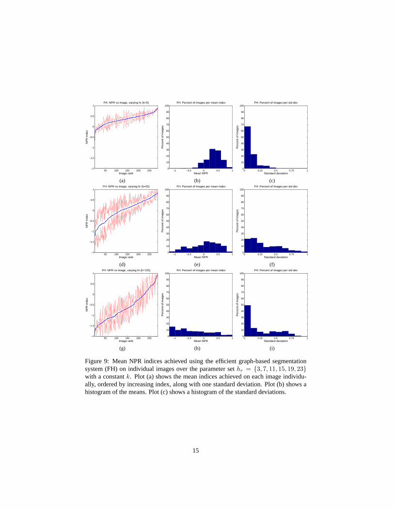
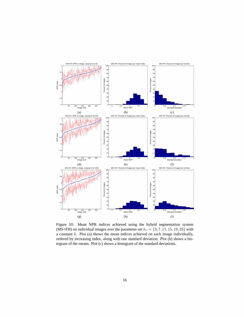
Although the above comparison is an interesting preliminary look at the data, it isactually biased since it is based on a different number of parameters for each algorithm,hence we now move on to more specific comparisons. This next comparison considersthe NPR indices averaged over values ofhr, with k held constant. The plots showingthis data for the EDISON method are the same as in the last section, in the first rowin Fig. 8. Fig. 9 gives the plots for the efficient graph-based segmentation system(FH) for k = {5, 25, 125}. We only show three out of the six values ofk in orderto keep the amount of data presented reasonable. Fig.10 gives the same informationfor the hybrid algorithm (MS+FH). The most interesting comparison here is betweenthe EDISON system and the hybrid system. We would like to judge what impact theaddition of the efficient graph-based clustering has had on the segmentations produced.

Notice that fork = 5, the performance of the hybrid (MS+FH) system in the firstrow of Fig. 10 is slightly better and certainly more stable than that of the mean shift-based (EDISON) system in Fig.8. For k = 25, in the second row of Fig.10, theperformance is more comparable, but the standard deviation is still somewhat lower.Finally, for k = 125, in the third row of Fig.10, the hybrid system performs compa-rably to the mean-shift based system. From these results we can see that the change tousing the efficient graph-based clustering after the mean shift filtering has maintainedthe correctness of the mean shift-based system while improving its stability.

Looking at the graphs for the efficient graph-based segmentation system alone inFig. 9, we can see that although fork = 5 the mean performance and standard deviationare promising, they quickly degrade for larger values ofk. This decline is much moregradual in the hybrid algorithm.

5.2.3 Average performance over different values ofk

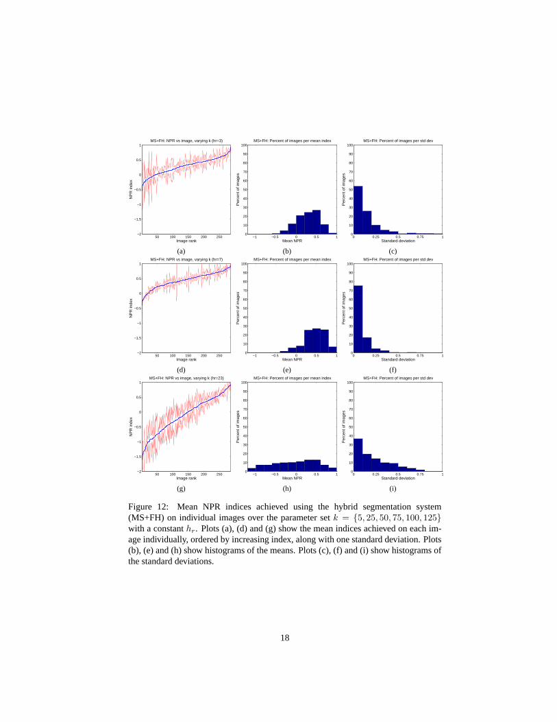
The final set of plots of this kind in figures Fig.11and Fig.12examine the mean NPRindices ask is varied throughk = {5, 25, 50, 75, 100, 125} andhr is held constant.Once again we only look at a representative three out of the six possiblehr values,hr = {3, 7, 23}. Since the mean shift-based system doesn’t usek, this comparison isbetween the efficient graph-based segmentation system and the hybrid system. It is im-mediately evident that the mean performance of the hybrid system is far superior to theefficient graph-based segmentation system, and that the results are much more stablewith respect to changing values ofk. Hence, adding a mean shift filtering preprocessingstep to the efficient graph-based segmentation system is clearly an improvement.

14

50 100 150 200 250−2

−1.5

−1

−0.5

0

0.5

1

Image rank

NP

R in

dex

FH: NPR vs image, varying hr (k=5)

−1 −0.5 0 0.5 10

10

20

30

40

50

60

70

80

90

100

Mean NPR

Per

cent

of i

mag

es


0 0.25 0.5 0.75 10

10

20

30

40

50

60

70

80

90

100

Standard deviation

Per

cent

of i

mag

es


(a) (b) (c)

50 100 150 200 250−2

−1.5

−1

−0.5

0

0.5

1

Image rank

NP

R in

dex


−1 −0.5 0 0.5 10

10

20

30

40

50

60

70

80

90

100

Mean NPR

Per

cent

of i

mag

es


0 0.25 0.5 0.75 10

10

20

30

40

50

60

70

80

90

100

Standard deviation

Per

cent

of i

mag

es


(d) (e) (f)

50 100 150 200 250−2

−1.5

−1

−0.5

0

0.5

1

Image rank

NP

R in

dex


−1 −0.5 0 0.5 10

10

20

30

40

50

60

70

80

90

100

Mean NPR

Per

cent

of i

mag

es


0 0.25 0.5 0.75 10

10

20

30

40

50

60

70

80

90

100

Standard deviation

Per

cent

of i

mag

es


(g) (h) (i)

Figure 9: Mean NPR indices achieved using the efficient graph-based segmentationsystem (FH) on individual images over the parameter sethr = {3, 7, 11, 15, 19, 23}with a constantk. Plot (a) shows the mean indices achieved on each image individu-ally, ordered by increasing index, along with one standard deviation. Plot (b) shows ahistogram of the means. Plot (c) shows a histogram of the standard deviations.

15

50 100 150 200 250−2

−1.5

−1

−0.5

0

0.5

1

Image rank

NP

R in

dex

MS+FH: NPR vs image, varying hr (k=5)

−1 −0.5 0 0.5 10

10

20

30

40

50

60

70

80

90

100

Mean NPR

Per

cent

of i

mag

es


0 0.25 0.5 0.75 10

10

20

30

40

50

60

70

80

90

100

Standard deviation

Per

cent

of i

mag

es


(a) (b) (c)

50 100 150 200 250−2

−1.5

−1

−0.5

0

0.5

1

Image rank

NP

R in

dex


−1 −0.5 0 0.5 10

10

20

30

40

50

60

70

80

90

100

Mean NPR

Per

cent

of i

mag

es


0 0.25 0.5 0.75 10

10

20

30

40

50

60

70

80

90

100

Standard deviation

Per

cent

of i

mag

es


(d) (e) (f)

50 100 150 200 250−2

−1.5

−1

−0.5

0

0.5

1

Image rank

NP

R in

dex


−1 −0.5 0 0.5 10

10

20

30

40

50

60

70

80

90

100

Mean NPR

Per

cent

of i

mag

es


0 0.25 0.5 0.75 10

10

20

30

40

50

60

70

80

90

100

Standard deviation

Per

cent

of i

mag

es


(g) (h) (i)

Figure 10: Mean NPR indices achieved using the hybrid segmentation system(MS+FH) on individual images over the parameter sethr = {3, 7, 11, 15, 19, 23} witha constantk. Plot (a) shows the mean indices achieved on each image individually,ordered by increasing index, along with one standard deviation. Plot (b) shows a his-togram of the means. Plot (c) shows a histogram of the standard deviations.

16

50 100 150 200 250−2

−1.5

−1

−0.5

0

0.5

1

Image rank

NP

R in

dex

FH: NPR vs image, varying k (hr=3)

−1 −0.5 0 0.5 10

10

20

30

40

50

60

70

80

90

100

Mean NPR

Per

cent

of i

mag

es


0 0.25 0.5 0.75 10

10

20

30

40

50

60

70

80

90

100

Standard deviation

Per

cent

of i

mag

es


(a) (b) (c)

50 100 150 200 250−2

−1.5

−1

−0.5

0

0.5

1

Image rank

NP

R in

dex


−1 −0.5 0 0.5 10

10

20

30

40

50

60

70

80

90

100

Mean NPR

Per

cent

of i

mag

es


0 0.25 0.5 0.75 10

10

20

30

40

50

60

70

80

90

100

Standard deviation

Per

cent

of i

mag

es


(d) (e) (f)

50 100 150 200 250−2

−1.5

−1

−0.5

0

0.5

1

Image rank

NP

R in

dex


−1 −0.5 0 0.5 10

10

20

30

40

50

60

70

80

90

100

Mean NPR

Per

cent

of i

mag

es


0 0.25 0.5 0.75 10

10

20

30

40

50

60

70

80

90

100

Standard deviation

Per

cent

of i

mag

es


(g) (h) (i)

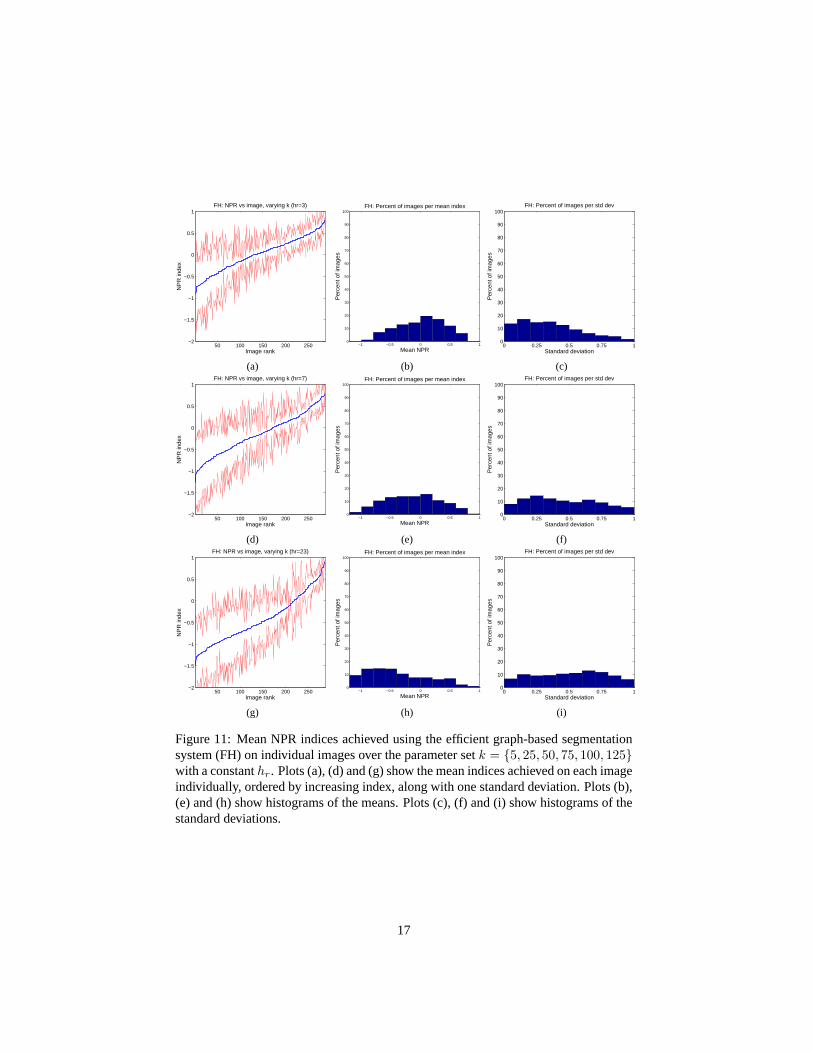
Figure 11: Mean NPR indices achieved using the efficient graph-based segmentationsystem (FH) on individual images over the parameter setk = {5, 25, 50, 75, 100, 125}with a constanthr. Plots (a), (d) and (g) show the mean indices achieved on each imageindividually, ordered by increasing index, along with one standard deviation. Plots (b),(e) and (h) show histograms of the means. Plots (c), (f) and (i) show histograms of thestandard deviations.

17

50 100 150 200 250−2

−1.5

−1

−0.5

0

0.5

1

Image rank

NP

R in

dex

MS+FH: NPR vs image, varying k (hr=3)

−1 −0.5 0 0.5 10

10

20

30

40

50

60

70

80

90

100

Mean NPRP

erce

nt o

f im

ages


0 0.25 0.5 0.75 10

10

20

30

40

50

60

70

80

90

100

Standard deviation

Per

cent

of i

mag

es


(a) (b) (c)

50 100 150 200 250−2

−1.5

−1

−0.5

0

0.5

1

Image rank

NP

R in

dex


−1 −0.5 0 0.5 10

10

20

30

40

50

60

70

80

90

100

Mean NPR

Per

cent

of i

mag

es


0 0.25 0.5 0.75 10

10

20

30

40

50

60

70

80

90

100

Standard deviation

Per

cent

of i

mag

es


(d) (e) (f)

50 100 150 200 250−2

−1.5

−1

−0.5

0

0.5

1

Image rank

NP

R in

dex


−1 −0.5 0 0.5 10

10

20

30

40

50

60

70

80

90

100

Mean NPR

Per

cent

of i

mag

es


0 0.25 0.5 0.75 10

10

20

30

40

50

60

70

80

90

100

Standard deviation

Per

cent

of i

mag

es


(g) (h) (i)

Figure 12: Mean NPR indices achieved using the hybrid segmentation system(MS+FH) on individual images over the parameter setk = {5, 25, 50, 75, 100, 125}with a constanthr. Plots (a), (d) and (g) show the mean indices achieved on each im-age individually, ordered by increasing index, along with one standard deviation. Plots(b), (e) and (h) show histograms of the means. Plots (c), (f) and (i) show histograms ofthe standard deviations.

18

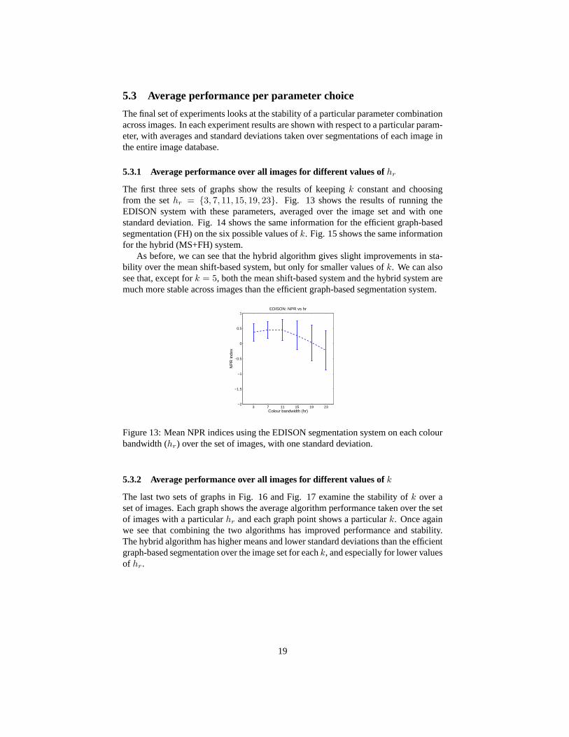
5.3 Average performance per parameter choice

The final set of experiments looks at the stability of a particular parameter combinationacross images. In each experiment results are shown with respect to a particular param-eter, with averages and standard deviations taken over segmentations of each image inthe entire image database.

5.3.1 Average performance over all images for different values ofhr

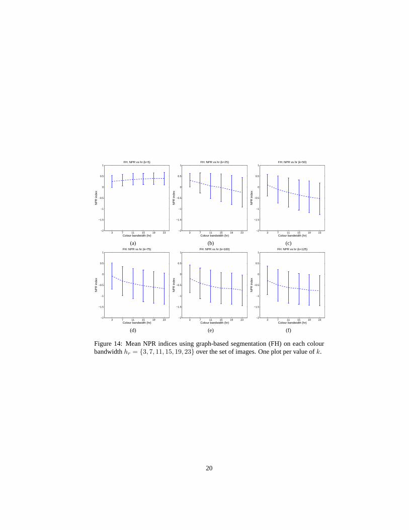
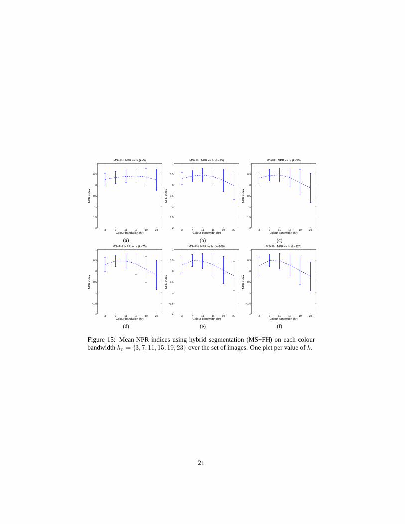
The first three sets of graphs show the results of keepingk constant and choosingfrom the sethr = {3, 7, 11, 15, 19, 23}. Fig. 13 shows the results of running theEDISON system with these parameters, averaged over the image set and with onestandard deviation. Fig.14 shows the same information for the efficient graph-basedsegmentation (FH) on the six possible values ofk. Fig. 15shows the same informationfor the hybrid (MS+FH) system.

As before, we can see that the hybrid algorithm gives slight improvements in sta-bility over the mean shift-based system, but only for smaller values ofk. We can alsosee that, except fork = 5, both the mean shift-based system and the hybrid system aremuch more stable across images than the efficient graph-based segmentation system.

3 7 11 15 19 23−2

−1.5

−1

−0.5

0

0.5

1

Colour bandwidth (hr)

NP

R in

dex

EDISON: NPR vs hr

Figure 13: Mean NPR indices using the EDISON segmentation system on each colourbandwidth (hr) over the set of images, with one standard deviation.

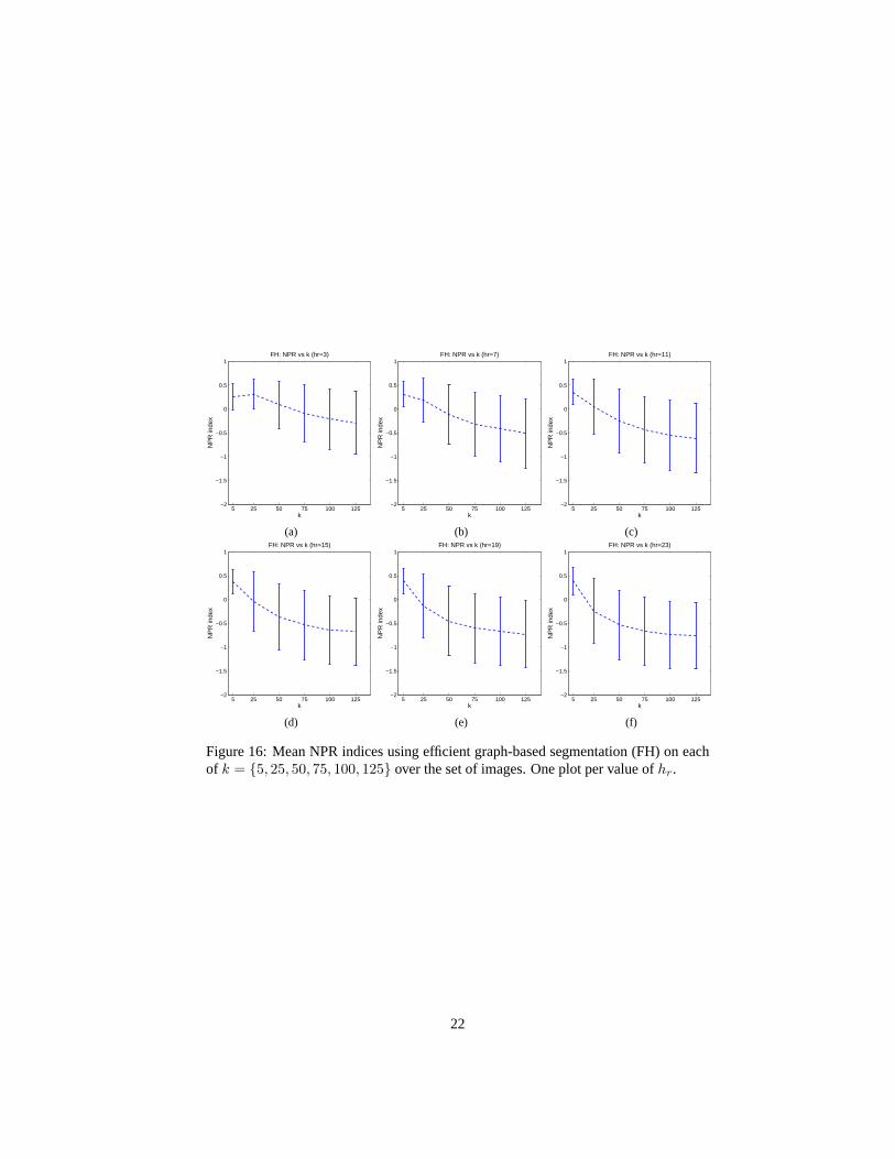
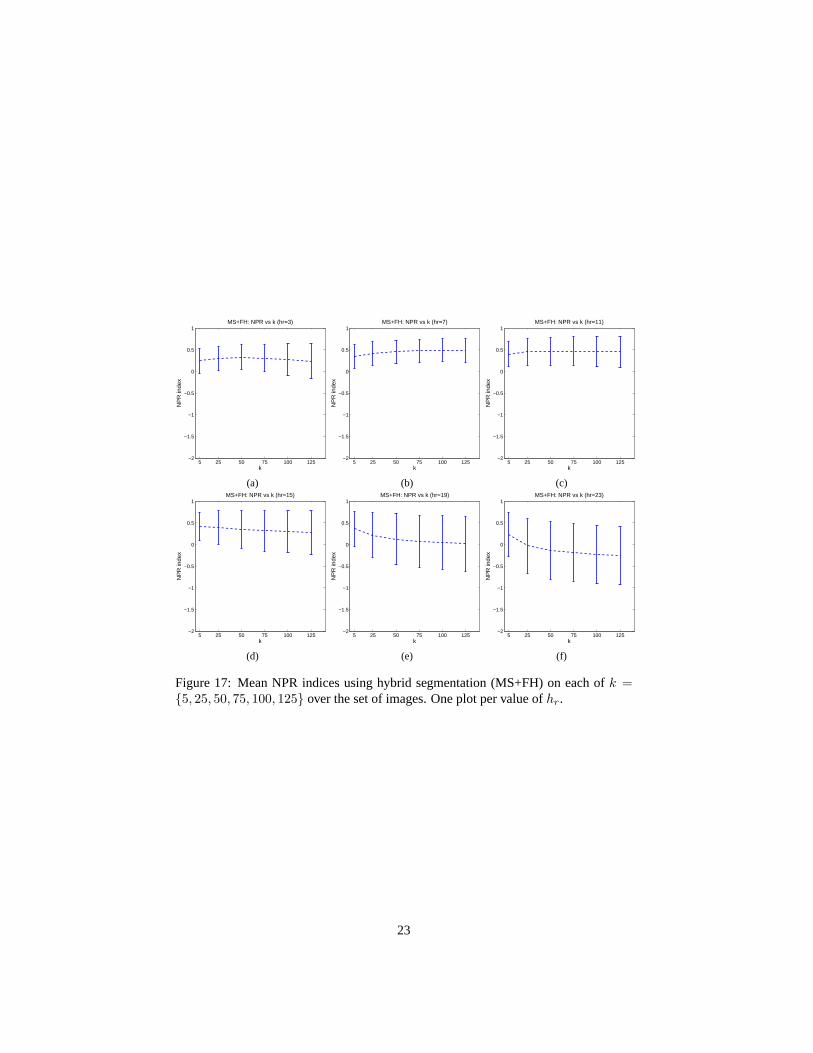
5.3.2 Average performance over all images for different values ofk

The last two sets of graphs in Fig.16 and Fig. 17 examine the stability ofk over aset of images. Each graph shows the average algorithm performance taken over the setof images with a particularhr and each graph point shows a particulark. Once againwe see that combining the two algorithms has improved performance and stability.The hybrid algorithm has higher means and lower standard deviations than the efficientgraph-based segmentation over the image set for eachk, and especially for lower valuesof hr.

19

3 7 11 15 19 23−2

−1.5

−1

−0.5

0

0.5

1


NP

R in

dex

FH: NPR vs hr (k=5)

3 7 11 15 19 23−2

−1.5

−1

−0.5

0

0.5

1


NP

R in

dex

FH: NPR vs hr (k=25)

3 7 11 15 19 23−2

−1.5

−1

−0.5

0

0.5

1


NP

R in

dex


(a) (b) (c)

3 7 11 15 19 23−2

−1.5

−1

−0.5

0

0.5

1


NP

R in

dex


3 7 11 15 19 23−2

−1.5

−1

−0.5

0

0.5

1


NP

R in

dex


3 7 11 15 19 23−2

−1.5

−1

−0.5

0

0.5

1


NP

R in

dex


(d) (e) (f)

Figure 14: Mean NPR indices using graph-based segmentation (FH) on each colourbandwidthhr = {3, 7, 11, 15, 19, 23} over the set of images. One plot per value ofk.

20

3 7 11 15 19 23−2

−1.5

−1

−0.5

0

0.5

1


NP

R in

dex

MS+FH: NPR vs hr (k=5)

3 7 11 15 19 23−2

−1.5

−1

−0.5

0

0.5

1


NP

R in

dex


3 7 11 15 19 23−2

−1.5

−1

−0.5

0

0.5

1


NP

R in

dex


(a) (b) (c)

3 7 11 15 19 23−2

−1.5

−1

−0.5

0

0.5

1


NP

R in

dex


3 7 11 15 19 23−2

−1.5

−1

−0.5

0

0.5

1


NP

R in

dex


3 7 11 15 19 23−2

−1.5

−1

−0.5

0

0.5

1


NP

R in

dex


(d) (e) (f)

Figure 15: Mean NPR indices using hybrid segmentation (MS+FH) on each colourbandwidthhr = {3, 7, 11, 15, 19, 23} over the set of images. One plot per value ofk.

21

5 25 50 75 100 125−2

−1.5

−1

−0.5

0

0.5

1

k

NP

R in

dex

FH: NPR vs k (hr=3)

5 25 50 75 100 125−2

−1.5

−1

−0.5

0

0.5

1

k

NP

R in

dex

FH: NPR vs k (hr=7)

5 25 50 75 100 125−2

−1.5

−1

−0.5

0

0.5

1

k

NP

R in

dex

FH: NPR vs k (hr=11)

(a) (b) (c)

5 25 50 75 100 125−2

−1.5

−1

−0.5

0

0.5

1

k

NP

R in

dex


5 25 50 75 100 125−2

−1.5

−1

−0.5

0

0.5

1

k

NP

R in

dex


5 25 50 75 100 125−2

−1.5

−1

−0.5

0

0.5

1

k

NP

R in

dex


(d) (e) (f)

Figure 16: Mean NPR indices using efficient graph-based segmentation (FH) on eachof k = {5, 25, 50, 75, 100, 125} over the set of images. One plot per value ofhr.

22

5 25 50 75 100 125−2

−1.5

−1

−0.5

0

0.5

1

k

NP

R in

dex

MS+FH: NPR vs k (hr=3)

5 25 50 75 100 125−2

−1.5

−1

−0.5

0

0.5

1

k

NP

R in

dex


5 25 50 75 100 125−2

−1.5

−1

−0.5

0

0.5

1

k

NP

R in

dex


(a) (b) (c)

5 25 50 75 100 125−2

−1.5

−1

−0.5

0

0.5

1

k

NP

R in

dex


5 25 50 75 100 125−2

−1.5

−1

−0.5

0

0.5

1

k

NP

R in

dex


5 25 50 75 100 125−2

−1.5

−1

−0.5

0

0.5

1

k

NP

R in

dex


(d) (e) (f)

Figure 17: Mean NPR indices using hybrid segmentation (MS+FH) on each ofk ={5, 25, 50, 75, 100, 125} over the set of images. One plot per value ofhr.

23

6 Summary and Conclusions

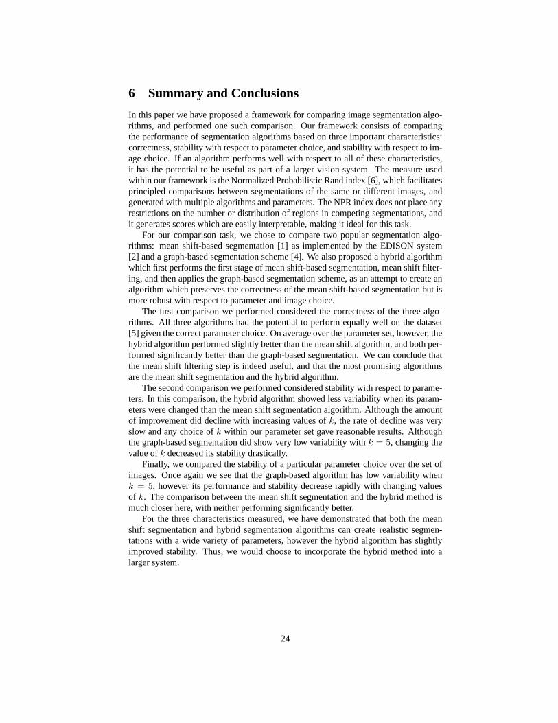
In this paper we have proposed a framework for comparing image segmentation algo-rithms, and performed one such comparison. Our framework consists of comparingthe performance of segmentation algorithms based on three important characteristics:correctness, stability with respect to parameter choice, and stability with respect to im-age choice. If an algorithm performs well with respect to all of these characteristics,it has the potential to be useful as part of a larger vision system. The measure usedwithin our framework is the Normalized Probabilistic Rand index [6], which facilitatesprincipled comparisons between segmentations of the same or different images, andgenerated with multiple algorithms and parameters. The NPR index does not place anyrestrictions on the number or distribution of regions in competing segmentations, andit generates scores which are easily interpretable, making it ideal for this task.

For our comparison task, we chose to compare two popular segmentation algo-rithms: mean shift-based segmentation [1] as implemented by the EDISON system[2] and a graph-based segmentation scheme [4]. We also proposed a hybrid algorithmwhich first performs the first stage of mean shift-based segmentation, mean shift filter-ing, and then applies the graph-based segmentation scheme, as an attempt to create analgorithm which preserves the correctness of the mean shift-based segmentation but ismore robust with respect to parameter and image choice.

The first comparison we performed considered the correctness of the three algo-rithms. All three algorithms had the potential to perform equally well on the dataset[5] given the correct parameter choice. On average over the parameter set, however, thehybrid algorithm performed slightly better than the mean shift algorithm, and both per-formed significantly better than the graph-based segmentation. We can conclude thatthe mean shift filtering step is indeed useful, and that the most promising algorithmsare the mean shift segmentation and the hybrid algorithm.

The second comparison we performed considered stability with respect to parame-ters. In this comparison, the hybrid algorithm showed less variability when its param-eters were changed than the mean shift segmentation algorithm. Although the amountof improvement did decline with increasing values ofk, the rate of decline was veryslow and any choice ofk within our parameter set gave reasonable results. Althoughthe graph-based segmentation did show very low variability withk = 5, changing thevalue ofk decreased its stability drastically.

Finally, we compared the stability of a particular parameter choice over the set ofimages. Once again we see that the graph-based algorithm has low variability whenk = 5, however its performance and stability decrease rapidly with changing valuesof k. The comparison between the mean shift segmentation and the hybrid method ismuch closer here, with neither performing significantly better.

For the three characteristics measured, we have demonstrated that both the meanshift segmentation and hybrid segmentation algorithms can create realistic segmen-tations with a wide variety of parameters, however the hybrid algorithm has slightlyimproved stability. Thus, we would choose to incorporate the hybrid method into alarger system.

24

References

[1] D. Comaniciu, P. Meer, “Mean shift: A robust approach toward feature spaceanalysis”, IEEE Trans. on Pattern Analysis and Machine Intelligence, 2002, 24,pp. 603-619

[2] C. Christoudias, B. Georgescu, P. Meer, “Synergism in Low Level Vision”, IntlConf on Pattern Recognition, 2002, 4, pp. 40190

[3] B. Georgescu, I. Shimshoni, P. Meer, “Mean Shift Based Clustering in High Di-mensions: A Texture Classification Example”, Intl Conf on Computer Vision,2003

[4] P. Felzenszwalb, D. Huttenlocher,“Efficient Graph-Based Image Segmentation”,Intl Journal of Computer Vision, 2004, 59 (2)

[5] D. Martin, C. Fowlkes, D. Tal, J. Malik, “A Database of Human Segmented Natu-ral Images and its Application to Evaluating Segmentation Algorithms and Mea-suring Ecological Statistics”, Intl Conf on Computer Vision, 2001.

[6] R. Unnikrishnan, C. Pantofaru, M. Hebert, “A Measure for Objective Evaluationof Image Segmentation Algorithms”, CVPR workshop on Empirical EvaluationMethods in Computer Vision, 2005.

[7] R. Unnikrishnan, M. Hebert, “Measures of Similarity”, IEEE Workshop on Com-puter Vision Applications, 2005, pp. 394–400.

[8] D. Verma, M. Meila, “A comparison of spectral clustering algorithms”, Univ ofWashington technical report, 2001.

[9] R. Kannan, S. Vempala, A. Vetta, “On clusterings - good, bad and spectral”,FOCS, 2000, pp. 367-377.

[10] M. Meila, J. Shi, “Learning segmentation by random walks”, NIPS, 2000,pp. 873-879.

[11] A. Y. Ng, M. I. Jordan, Y. Weiss, “On spectral clustering: Analysis and an algo-rithm”, NIPS, 2002, pp. 849-856.

[12] M. Meila, “Comparing clusterings”, Univ of Washington Technical Report, 2002.

[13] J. Shi, J. Malik, “Normalized cuts and image segmentation”, IEEE Transactionson Pattern Analysis and Machine Learning, 2000, pp. 888-905.

[14] D. Martin, “An Empirical Approach to Grouping and Segmentation”, Ph.D. dis-sertation, 2002, University of California, Berkeley.

25

Documents

A Comparison of Image Segmentation Algorithms · A Comparison of Image Segmentation Algorithms ... A system designer now has an array of available algorithm choices, how- ... mentation