Embed Size (px)
Citation preview
Biomech Model Mechanobiol (2012) 11:519–532DOI 10.1007/s10237-011-0330-2
ORIGINAL PAPER
A comparison of models of the isometric force of locust skeletalmuscle in response to pulse train inputs
Emma Wilson · Emiliano Rustighi ·Philip L. Newland · Brian R. Mace
Received: 7 March 2011 / Accepted: 25 June 2011 / Published online: 8 July 2011© Springer-Verlag 2011
Abstract Muscle models are an important tool in thedevelopment of new rehabilitation and diagnostic techniques.Many models have been proposed in the past, but little workhas been done on comparing the performance of models. Inthis paper, seven models that describe the isometric forceresponse to pulse train inputs are investigated. Five of themodels are from the literature while two new models are alsopresented. Models are compared in terms of their ability to fitto isometric force data, using Akaike’s and Bayesian infor-mation criteria and by examining the ability of each model todescribe the underlying behaviour in response to individualpulses. Experimental data were collected by stimulating thelocust extensor tibia muscle and measuring the force gener-ated at the tibia. Parameters in each model were estimated byminimising the error between the modelled and actual forceresponse for a set of training data. A separate set of test data,which included physiological kick-type data, was used to as-sess the models. It was found that a linear model performedthe worst whereas a new model was found to perform thebest. The parameter sensitivity of this new model was inves-tigated using a one-at-a-time approach, and it found that theforce response is not particularly sensitive to changes in anyparameter.
Keywords Muscle model · Isometric · Muscle force ·Locust extensor muscle
E. Wilson (B) · E. Rustighi · B. R. MaceInstitute of Sound and Vibration Research,University of Southampton, Southampton,Hampshire SO17 1BJ, UKe-mail: [email protected]
P. L. NewlandSchool of Biological Sciences,University of Southampton, Southampton,Hampshire SO17 1BJ, UK
1 Introduction
Muscles act as actuators that do the work in moving theskeleton (Meijer et al. 2001). Musculoskeletal modelling hasuses in controlling movement, such as in functional electri-cal stimulation (FES), as well as helping to build devicesthat restore function after injury (Freeman et al. 2009; Rosenet al. 2001). A mathematical model highlights the importantfunctions of the muscle and can provide predictive insightinto the behaviour. An accurate, predictive model can help todrive FES protocol.
In the present study, the locust hind leg extensor tibia(ETi) muscle is studied. Invertebrate muscle has receivedmuch less attention to date than vertebrate muscle; how-ever, the muscles share fundamental similarities with cal-cium being the key regulatory factor (Ebashi 1980). Themuscles of vertebrates and invertebrates differ in terms oftheir innervation. Invertebrate muscle is innervated by a muchsmaller set of neurones that are often identifiable (Hoyle1955; Theophilidis and Burns 1983). The locust hind legETi muscle is innervated by two excitatory neurones; neu-ral events leading to contraction are tractable and relativelyeasily produced during experiment.
Despite the processes behind muscle contraction beingreasonably well established (Huxley 1985), no single broadlyaccepted method of modelling skeletal muscle exists(Valero-Cuevas et al. 2009). Developed models and theirlevel of simplicity tend to depend upon the research ques-tions, and so on a specific goal or task (Winters 1995), hence,important model properties are task specific. A Hill-typemodel is a more commonly used model (Christophy et al.2011). However, Hill-type models do not tend to describe thechemo-mechanical energy conversion processes that occurduring the transformation from an action potential to force(Repperger et al. 2006) and so have limited use in terms of
123
520 E. Wilson et al.
modelling the isometric behaviour. The lack of a standardisedmodelling approach is partly a result of researchers tendingto use solely their own model and of the varying simplifyingassumptions used to reduce the complexity of the muscle sys-tem made in various studies. By studying a simply innervatedmuscle, the complexity of the muscle system is minimisedin this study.
Few studies compare the validity of different types ofmodel (Bobet et al. 2005). Due to the lack of comparativestudies, it is difficult to establish which model is most appro-priate and to determine whether a simpler model would be asgood at describing the behaviour. To the authors knowledge,only two previous studies compare a range of different mod-els (Bobet et al. 2005; Law and Shields 2005). Furthermore,of these, only Bobet et al. (2005) compare models by fittingto measured data. In this study, the innovative work of Bobetet al. (2005) is extended. The ability of a new Adapted model(Wilson et al. 2011) to predict the isometric force responseto pulse train inputs is assessed alongside a range of existingmodels in the literature. Models considered in the compari-son include a Linear model (Baratta and Solomonow 1990;Mannard and Stein 1973), Wiener model (Bobet et al. 2005),Cascade model (Ghigliazza and Holmes 2005; Hatze 1977),the model of Ding et al. (2002), and the model of Bobetand Stein (1998), and new Adapted and Simplified Adaptedmodels (Wilson et al. 2011; Wilson 2011). Modelling capa-bilities are compared by considering goodness of fits in theleast squares sense, as was done by Bobet et al. (2005). Thisapproach is extended to also consider the ability of models topredict the underlying behaviour and by using Akaike’s andBayesian information criteria (AIC and BIC, respectively).
In this study, a simple task, modelling the isometric forceresponse of the locust hind leg extensor muscle to input pulsesis considered. The best model is taken to be the model that ismost capable of simulating the force measured during exper-iments with minimal complexity. This measure of best isquantified by the goodness of fit (error measurement) andAIC and BIC. Since models were evaluated with respect totheir capability of describing the isometric force developedby a locust muscle in response to FETi stimulation, the bestmodel is likely to be more directly applicable to describ-ing the isometric force response of invertebrate muscle tofast motor neurone stimulation. Hence, the best model hasthe potential to provide a better actuation strategy for thedevelopment of robotic devices such as hexaped robots. Themodels were assessed by their ability to describe the forcedeveloped by a particular muscle in a particular species wherethe effect of movement is not included, this does not provideenough information to conclude that the model is the best forall kinds of musculoskeletal modelling. However, the sim-plicity of the muscle system from which data to evaluatethe candidate models is obtained means that the best model
may provide a good building block for modelling systems ofincreased complexity.
In the next section, the methods used to measure the forceresponse of the muscle are described, with details of the inputstimulation patterns provided. Mathematical descriptions ofthe candidate models are then presented. The capability ofthese models to describe the force response of the muscle isthen assessed, and a sensitivity analysis performed on the bestmodel, the Adapted model. A discussion of this model andconclusions from the comparative study are then provided.
2 Methods
2.1 Force measurements
Adult locusts (Schistocerca gregaria, Forskål) of both sexes,taken from a colony at the University of Southampton, wereused for experiments. Locusts were securely fixed ventralside up using modelling clay. The left (looking from ventralside, with head at top) hind leg was clamped ventral side up sothat the femur was fixed but the tibia and tarsi of the leg werefree to move with their full range (Burrows and Horridge1974). The femoral-tibial (FT) angle was set to 80◦ using aprotractor, with a pin used to hold the tibia at 80◦. Duringexperiments, the muscle was held isometric by constrainingthe angle. Further discussion of the isometric assumption isprovided in Wilson et al. (2010, 2011), Wilson (2011).
The ETi muscle was stimulated by implanted electrodes.Hoyle (1978) described precisely the innervation pattern ofETi. We therefore always implanted the stimulation elec-trodes in the same position in each locust. The electrodeswere inserted through the sixth attachment point from theproximal end of the femur, on the anterior surface (corre-sponding to outside region c in Hoyle 1978). The ETi is inner-vated by four axons (Hoyle 1978); a fast (FETi) and slow(SETi) excitatory motor neurone, a common inhibitor (CI)and a dorsal unpaired median (DUMETi). In region c fibresare innervated by only FETi and DUMETi (Hoyle 1978). Torule out potential confounding factors, caused by multiplemotor neurones being activated, we performed preliminaryexperiments in which the stimulus duration was held con-stant at 3 ms and the stimulus pulse amplitude was increaseduntil a single, unitary amplitude response was elicited. Sim-ilar amplitude levels (5 V) with pulse durations of 3 ms werethen used in experiments. This is expected to lead to activa-tion of only FETi as its diameter is approximately 10 timesgreater than that of DUMETi in region c (Hoyle 1978). How-ever, we did not carry out further tests to identify FETi activ-ity precisely, so it remains possible that other motor neuronesmight also be activated during muscle stimulation. Any prep-arations in which there was a clear change in the twitch force
123
A comparison of models of the isometric force 521
during experiment, suggesting additional innervation, wereomitted from results.
An S100 SMD thin film load cell with range up to 1 N wasused to measure the force at the tibia. The output of the loadcell was fed into a Fylde FE-369-TA transducer amplifier toamplify and filter the signal prior to acquisition. The filtercut-off frequency was set to 1 kHz (−3 dB). Both the inputto the muscle, and the load cell output, were recorded with asampling frequency of 2.2 kHz. The recorded force was nor-malised by dividing by the maximum tetanic force (recordedduring a 40 pulse, 67 Hz train of input pulses) for each locust.All results presented refer to normalised force obtained usingthis method. For further details on the experimental set up,refer to Wilson et al. (2010), Wilson (2011).
2.2 Stimulation protocol
Previous work found that the input stimulation pulses couldbe assumed to be equivalent to impulses (Wilson et al. 2011).The ability of a range of models to capture the isometric forceresponse to a pulse train input of the form
u(t) =n∑
i=1
δ(t − ti ) (1)
is assessed. To assess model performance, parameters wereestimated using a training data set, and the performanceevaluated using a different test data set. The set of train-ing data was chosen to be rich enough in content so thatit provided small errors when fitting to test data, includingphysiologically relevant data, whilst keeping the quan-tity of input data low. Training data consisted of 5 iso-lated pulses, a 40-pulse constant-frequency train (CFT)with interpulse frequency (IPF) of 66.7 Hz, a pulse trainof 29 pulses which increased then decreased in frequency(back to initial value), with a maximum frequency of100 Hz and minimum of 10 Hz, and a 60 pulse train whichdecreased then increased in frequency (back to the startvalue) with a minimum frequency of 1 Hz and maximumof 50 Hz.
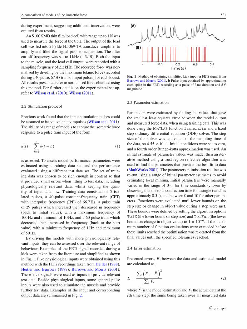
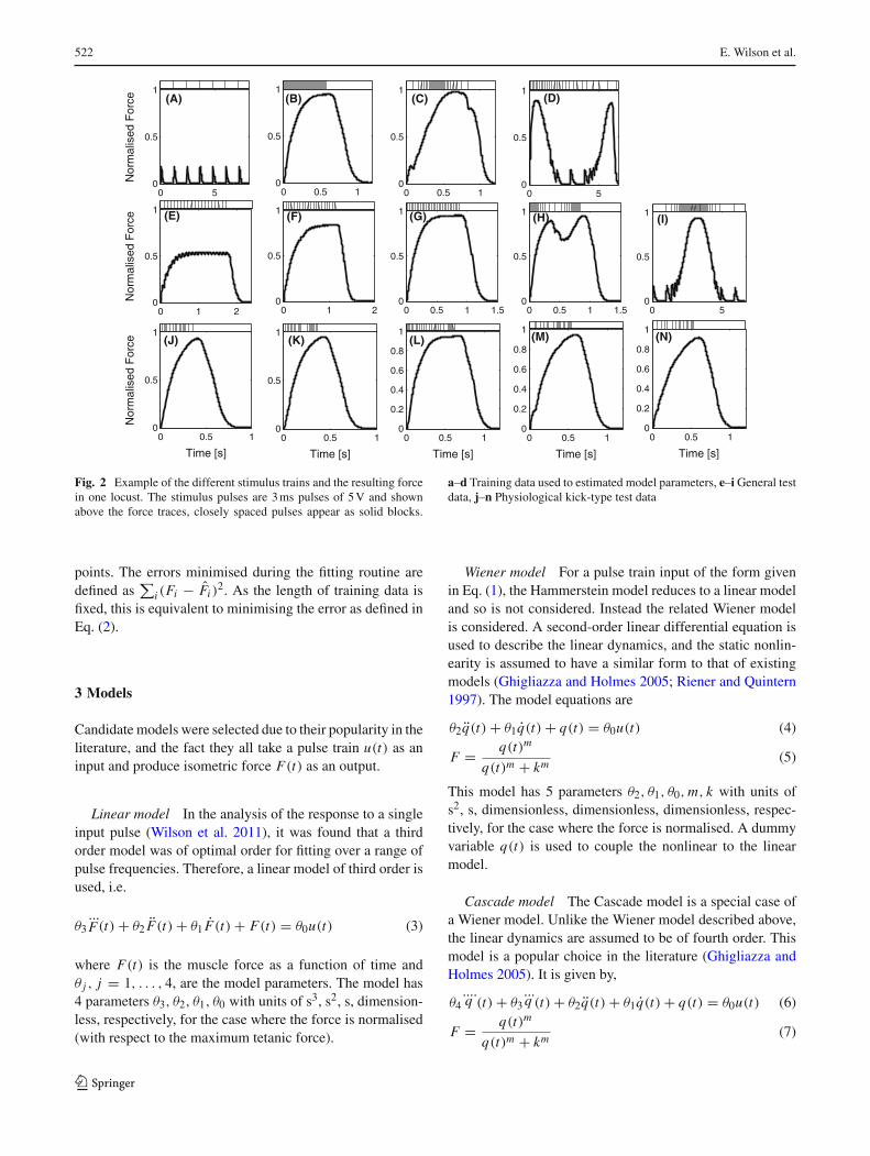
By driving the models with more physiologically rele-vant inputs, they can be assessed over the relevant range ofbehaviour. Examples of the FETi signal recorded during akick were taken from the literature and simplified as shownin Fig. 1. Five physiological inputs were obtained using thismethod with the FETi recordings taken from Heitler (1988),Heitler and Burrows (1977), Burrows and Morris (2001).These kick signals were used as inputs to provide relevanttest data. Beside physiological inputs, some general pulseinputs were also used to stimulate the muscle and providefurther test data. Examples of the input and correspondingoutput data are summarised in Fig. 2.
Fig. 1 Method of obtaining simplified kick input, a FETi signal fromBurrows and Morris (2001), b Pulse input obtained by approximatingeach spike in the FETi recording as a pulse of 3 ms duration and 5 Vmagnitude
2.3 Parameter estimation
Parameters were estimated by finding the values that gavethe smallest least squares error between the model outputand measured force data, when using training data. This wasdone using the Matlab function lsqnonlin and a fixedstep ordinary differential equation (ODE) solver. The stepsize of the solver was equivalent to the sampling time ofthe data, so 4.55 × 10⁻⁴. Initial conditions were set to zero,and a fourth order Runge-kutta approximation was used. Aninitial estimate of parameter values was made, then an iter-ative method using a trust-region-reflective algorithm wasused to find the parameters that provide the best fit to data(MathWorks 2001). The parameter optimisation routine wasre-run using a range of initial parameter estimates to avoidestimating local minima. Initial parameters were manuallyvaried in the range of 0–1 for time constants (chosen byobserving that the total contraction time for a single twitch isapproximately 0.5 s), and between 0 and 10 for other param-eters. Functions were evaluated until lower bounds on thestep size or change in object value during a step were met.These bounds were defined by setting the algorithm optionsTolX (the lower bound on step size) and TolFun (the lowerbound on change in object value) to 1 × 10⁻⁶. If the maxi-mum number of function evaluations were exceeded beforethese limits reached the optimisation was re-started from thefinal values until the specified tolerances reached.
2.4 Error estimation
Presented errors, E , between the data and estimated modelare calculated as,
E =∑
i
(Fi − Fi
)2
∑i Fi
(2)
where Fi is the model estimation and Fi the actual data at thei th time step, the sums being taken over all measured data
123
522 E. Wilson et al.
0 50
0.5
1(A)
Nor
mal
ised
For
ce
0 0.5 10
0.5
1(B)
0 0.5 10
0.5
1(C)
0 50
0.5
1(D)
0 1 20
0.5
1
Nor
mal
ised
For
ce (E)
0 1 20
0.5
1 (F)
0 0.5 1 1.50
0.5
1 (G)
0 50
0.5
1(I)
0 0.5 1 1.50
0.5
1 (H)
0 0.5 10
0.5
1
Time [s]
Nor
mal
ised
For
ce (J)
0 0.5 10
0.5
1(K)
Time [s]
0 0.5 10
0.2
0.4
0.6
0.8
1(L)
Time [s]
0 0.5 10
0.2
0.4
0.6
0.8
1(M)
Time [s]
0 0.5 10
0.2
0.4
0.6
0.8
1
Time [s]
(N)
Fig. 2 Example of the different stimulus trains and the resulting forcein one locust. The stimulus pulses are 3 ms pulses of 5 V and shownabove the force traces, closely spaced pulses appear as solid blocks.
a–d Training data used to estimated model parameters, e–i General testdata, j–n Physiological kick-type test data
points. The errors minimised during the fitting routine aredefined as
∑i (Fi − Fi )
2. As the length of training data isfixed, this is equivalent to minimising the error as defined inEq. (2).
3 Models
Candidate models were selected due to their popularity in theliterature, and the fact they all take a pulse train u(t) as aninput and produce isometric force F(t) as an output.
Linear model In the analysis of the response to a singleinput pulse (Wilson et al. 2011), it was found that a thirdorder model was of optimal order for fitting over a range ofpulse frequencies. Therefore, a linear model of third order isused, i.e.
θ3...F(t) + θ2 F(t) + θ1 F(t) + F(t) = θ0u(t) (3)
where F(t) is the muscle force as a function of time andθ j , j = 1, . . . , 4, are the model parameters. The model has4 parameters θ3, θ2, θ1, θ0 with units of s3, s2, s, dimension-less, respectively, for the case where the force is normalised(with respect to the maximum tetanic force).
Wiener model For a pulse train input of the form givenin Eq. (1), the Hammerstein model reduces to a linear modeland so is not considered. Instead the related Wiener modelis considered. A second-order linear differential equation isused to describe the linear dynamics, and the static nonlin-earity is assumed to have a similar form to that of existingmodels (Ghigliazza and Holmes 2005; Riener and Quintern1997). The model equations are
θ2q(t) + θ1q(t) + q(t) = θ0u(t) (4)
F = q(t)m
q(t)m + km(5)
This model has 5 parameters θ2, θ1, θ0, m, k with units ofs2, s, dimensionless, dimensionless, dimensionless, respec-tively, for the case where the force is normalised. A dummyvariable q(t) is used to couple the nonlinear to the linearmodel.
Cascade model The Cascade model is a special case ofa Wiener model. Unlike the Wiener model described above,the linear dynamics are assumed to be of fourth order. Thismodel is a popular choice in the literature (Ghigliazza andHolmes 2005). It is given by,
θ4....q (t) + θ3
...q (t) + θ2q(t) + θ1q(t) + q(t) = θ0u(t) (6)
F = q(t)m
q(t)m + km(7)
123
A comparison of models of the isometric force 523
This model has 7 parameters, θ4, θ3, θ2, θ1, θ0, m, k withunits of s4, s3, s2, s, dimensionless, dimensionless,dimensionless, respectively, for the case where the force isnormalised. The variable q(t) is a dummy variable, used tocouple the nonlinear and linear equations. The variable q(t) iscommonly assumed to represent the calcium release from thesarcoplasmic reticulum (SR) (Ghigliazza and Holmes 2005).It is often the case that the linear dynamics (Eq. 6) are writtenas two coupled second-order ODEs, with the T-tubuli depo-larisation response given as an intermediate step to findingthe calcium release (Ghigliazza and Holmes 2005).
Ding et al model Ding et al. (2002) find their model givesgood fits to data. It is given by
q(t) + q(t)
τc= u(t) (8)
CN (t) + CN (t)
τc= q(t)
τc
n∑
i
Ri (9)
x(t) = CN (t)
k + CN (t)(10)
F(t) + F(t)
τ1 + τ2x(t)= Ax(t) (11)
Ri = 1 + (Ro − 1) exp
(−(ti − ti−1)
τc
)(12)
This model has 6 parameters, τc, τ1, τ2, A, Ro, k with unitsof s, s, s, s−1, dimensionless, dimensionless, respectively,for the case where the force is normalised. The variablesRi , CN (t), q(t) and x(t) are intermediate stages in the model.The variable q(t) is used as an intermediate in calculatingCN (t), which is said to represent the normalised amount ofthe Ca2+ complex. The variable x(t) describes the non-lin-ear saturation, and Ri (dimensionless) is used to account fornonlinear summation when the muscle is stimulated by twoclosely spaced pulses, where ti defines the time of the i thstimulation.
Bobet and Stein model Bobet and Stein (1998) present amodel that they find to provide good fits to the force producedby cat muscle. The model is
q(t) + aq(t) = u(t) (13)
x(t) = q(t)m
q(t)m + km(14)
F(t) + bF(t) = Bbx(t) (15)
b = bo
(1 − b1 F(t)
B
)2
(16)
This model has 6 parameters, a, m, k, bo, b1, B with unitsof s−1, dimensionless, dimensionless, s−1, dimensionless,dimensionless, respectively, for the case where the force isnormalised. The parameter a is thought to represent the decayof free calcium concentration; m and k define a nonlinearity
that might represent the binding of calcium ions to troponin,and B is a scale factor. The nonlinearity in Eq. (15) that arisesfrom the definition of b (Eq. 16) is thought to represent thedecay of force under different conditions.
Adapted model The model of Ding et al. (2002) wasadapted to give a model of similar, yet simpler form to thatof Bobet and Stein (1998). This new, ‘Adapted model’ ispresented in Wilson et al. (2011). The Adapted model is,
CN (t) + CN (t)
τc= u(t) (17)
x(t) = CN (t)m
CN (t)m + km(18)
F(t) + F(t)
τ1 + τ2x(t)= Ax(t) (19)
This model has 6 parameters, τc, τ1, τ2, m, k, A. For the casewhere F(t) is normalised, the time constants τ1, τ2 and τc
have units of s, A units of s−1, while all other parametersare dimensionless. The development of the Adapted modelis discussed in the following section.
Simplified adapted model The Adapted model was sim-plified, by assuming the parameter τ2 = 0 as discussed inthe subsequent section, giving the following model
CN (t) + CN (t)
τc= u(t) (20)
x(t) = CN (t)m
CN (t)m + km(21)
F(t) + F(t)
τ1= Ax(t). (22)
3.1 The adapted model
The Adapted and Simplified models are described in moredetail here. These models were adapted from the model ofDing et al. (2002). The model of Ding et al. (2002) (describedby Eqs. (8–12) provides reasonable fits to data; however, thephysiological meaning of the model and parameters is hard tointerpret. A sensitivity analysis by Law and Shields (2005)that looked at trying to better understand the relationshipbetween model parameters and muscle contractile proper-ties found the parameter definitions of Ding et al. (2002) toonly be partially supported. Furthermore, no physical reasonwas given or could be found, as to why the time constantsin Eqs. (8) and (9) should be the same. Therefore, as a firststep, a model variation in which the time constant in Eq. (8)was allowed to differ from that in Eq. (9) was investigated,
123
524 E. Wilson et al.
0
1
0.5
CN
x(t
)
Increasing m
k
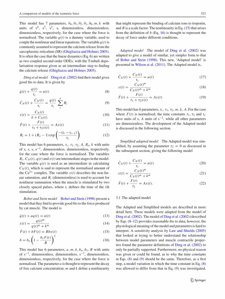
Fig. 3 The change in saturation nonlinearity (Eq. 21) with m
giving the model the following form,
q(t) + q(t)
τR= u(t) (23)
CN (t) + CN (t)
τc= q(t)
τc
n∑
i
Ri (24)
x(t) = CN (t)
k + CN (t)(25)
F(t) + F(t)
τ1 + τ2x(t)= Ax(t) (26)
Ri = 1 + (Ro − 1) exp
(−(ti − ti−1)
τc
)(27)
This introduces an extra parameter τR . It was found thatthe resultant fit was insensitive to the value of the parame-ter τR and good fits could be obtained for a range of valuesof τR . The original model was thus simplified in an attemptto reduce parameter redundancy and to make the essentialcharacteristics of the model clearer. The resultant model isgiven as Eqs. (17)–(19) and termed the Adapted model. Inthe Adapted model, the order of the model is reduced andthe parameter τR neglected, hence the state variable q(t) isnot required. The relation between input and output is sec-ond rather than third order. The variable Ri , which was saidto account for the non-linear summation in response to twoclosely spaced pulses, has been removed. Instead, an extraparameter, m is included to allow the specific form of thenonlinearity to change. Figure 3 shows how the saturationcurve changes with the value of m.
In a previous paper, we investigated the response to eachindividual pulse in a CFT that sum to make up the totalresponse (Wilson et al. 2011). It was found that the responsesdiffered dependent on the pulse number or IPF. The Adaptedmodel is able to capture the fundamentals of the underlyingbehaviour of each individual pulse and so is considered as acandidate model. The Simplified Adapted model was devel-oped from the Adapted model by assuming that τ2 = 0.Under this assumption, the model is still capable of describ-ing the fundamentals of the underlying behaviour (responseto each stimulus) so therefore the Simplified Adapted modelis also used as a candidate model. Equations describing theSimplified Adapted model are given as Eqs. (20–22).
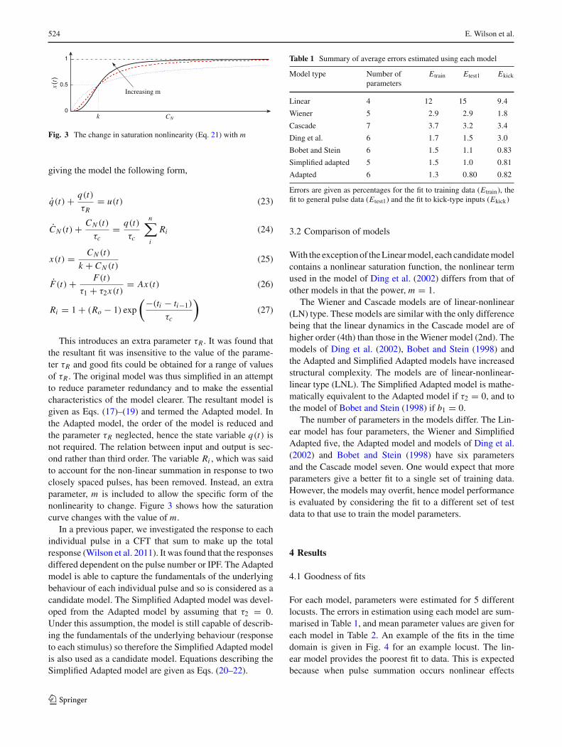
Table 1 Summary of average errors estimated using each model
Model type Number ofparameters
Etrain Etest1 Ekick
Linear 4 12 15 9.4
Wiener 5 2.9 2.9 1.8
Cascade 7 3.7 3.2 3.4
Ding et al. 6 1.7 1.5 3.0
Bobet and Stein 6 1.5 1.1 0.83
Simplified adapted 5 1.5 1.0 0.81
Adapted 6 1.3 0.80 0.82
Errors are given as percentages for the fit to training data (Etrain), thefit to general pulse data (Etest1) and the fit to kick-type inputs (Ekick)
3.2 Comparison of models
With the exception of the Linear model, each candidate modelcontains a nonlinear saturation function, the nonlinear termused in the model of Ding et al. (2002) differs from that ofother models in that the power, m = 1.
The Wiener and Cascade models are of linear-nonlinear(LN) type. These models are similar with the only differencebeing that the linear dynamics in the Cascade model are ofhigher order (4th) than those in the Wiener model (2nd). Themodels of Ding et al. (2002), Bobet and Stein (1998) andthe Adapted and Simplified Adapted models have increasedstructural complexity. The models are of linear-nonlinear-linear type (LNL). The Simplified Adapted model is mathe-matically equivalent to the Adapted model if τ2 = 0, and tothe model of Bobet and Stein (1998) if b1 = 0.
The number of parameters in the models differ. The Lin-ear model has four parameters, the Wiener and SimplifiedAdapted five, the Adapted model and models of Ding et al.(2002) and Bobet and Stein (1998) have six parametersand the Cascade model seven. One would expect that moreparameters give a better fit to a single set of training data.However, the models may overfit, hence model performanceis evaluated by considering the fit to a different set of testdata to that use to train the model parameters.
4 Results
4.1 Goodness of fits
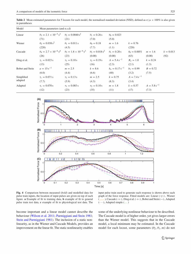
For each model, parameters were estimated for 5 differentlocusts. The errors in estimation using each model are sum-marised in Table 1, and mean parameter values are given foreach model in Table 2. An example of the fits in the timedomain is given in Fig. 4 for an example locust. The lin-ear model provides the poorest fit to data. This is expectedbecause when pulse summation occurs nonlinear effects
123
A comparison of models of the isometric force 525
Table 2 Mean estimated parameters for 5 locusts for each model, the normalised standard deviation (NSD), defined as σ/μ × 100% is also givenin parentheses
Model Mean parameters (and n.s.d)
Linear θ3 = 2.1 × 10⁻⁵ s3 θ2 = 0.0040 s2 θ1 = 0.26 s θ0 = 0.023
(71) (21) (7.0) (5.0)
Wiener θ2 = 0.038 s2 θ1 = 0.011 s θ0 = 0.18 m = 1.6 k = 0.76
(220) (4.5) (7.7) (1.1) (220)
Cascade θ4 = 2.7 × 10⁻⁶ s4 θ3 = 1.8 × 10⁻⁴ s3 θ2 = 0.018 s2 θ1 = 0.20 s θ0 = 0.0051 m = 1.6 k = 0.013
(26) (23) (0.00) (0.00) (63) (0.00) (92)
Ding et al. τc = 0.023 s τ1 = 0.10 s τ2 = 0.19 s A = 5.4 s−1 Ro = 1.0 k = 0.24
(13) (25) (16) (2.3) (2.1) (1.3)
Bobet and Stein a = 15 s−1 m = 2.5 k = 8.6 bo = 0.17 s−1 b1 = 0.99 B = 0.72
(6.0) (4.4) (6.6) (40) (3.2) (7.5)
Simplifiedadapted
τc = 0.071 s τ1 = 0.13 s m = 2.5 k = 0.75 A = 7.4 s−1
(7.7) (5.9) (4.3) (8.3) (3.4)
Adapted τc = 0.070 s τ1 = 0.083 s τ2 = 0.10 s m = 1.8 k = 0.57 A = 5.8 s−1
(12) (23) (35) (11) (17) (7.3)
0 1 2 3 4 5 60
0.5
1
Nor
mal
ised
For
ce
(A)
(B)
0 0.2 0.4 0.6 0.8 1 1.20
0.5
1
Nor
mal
ised
For
ce
(C)
0 0.1 0.2 0.3 0.4 0.5 0.6 0.7 0.8 0.9 10
0.5
1
Time [s]
Nor
mal
ised
For
ce
Fig. 4 Comparison between measured (bold) and modelled data forpulse train inputs, the location of input pulses are given on top of eachfigure. a Example of fit to training data, b example of fit to generalpulse train test data, c example of fit to physiological test data. The
input pulse train used to generate each response is shown above eachgraph of the force response. Fitted models are: Linear (-�-) , Wiener( ), Cascade (-×-) , Ding et al. (-+-) , Bobet and Stein (—) , Adapted(- - -), Adapted simple ( )
become important and a linear model cannot describe thebehaviour (Wilson et al. 2011; Parmiggiani and Stein 1981;Stein and Parmiggiani 1981). The inclusion of a static non-linearity, as in the Wiener and Cascade Models, provides animprovement on the linear fit. The static nonlinearity enables
some of the underlying nonlinear behaviour to be described.The Cascade model is of higher order, yet gives larger errorsthan the Wiener model. This suggests that in the Cascademodel, a local minimum may be estimated. In the Cascademodel for each locust, some parameters (θ2, θ1, m) do not
123
526 E. Wilson et al.
0 1 2 3 4 5 60
0.5
1
Nor
mal
ised
For
ce
(A)
(B)
0 0.2 0.4 0.6 0.8 1 1.20
0.5
1
Nor
mal
ised
For
ce
(C)
0 0.1 0.2 0.3 0.4 0.5 0.6 0.7 0.8 0.9 10
0.5
1
Time [s]
Nor
mal
ised
For
ce
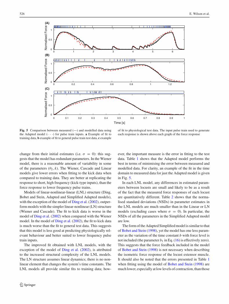
Fig. 5 Comparison between measured (—) and modelled data usingthe Adapted model (- - -) for pulse train inputs. a Example of fit totraining data, b example of fit to general pulse train test data, c example
of fit to physiological test data. The input pulse train used to generateeach response is shown above each graph of the force response
change from their initial estimates (i.e. σ = 0): this sug-gests that the model has redundant parameters. In the Wienermodel, there is a reasonable amount of variability in someof the parameters (θ2, k). The Wiener, Cascade and Linearmodels give lower errors when fitting to the kick data whencompared to training data. They are better at replicating theresponse to short, high frequency (kick-type inputs), than theforce response to lower frequency pulse trains.
Models of linear-nonlinear-linear (LNL) structure (Ding,Bobet and Stein, Adapted and Simplified Adapted models),with the exception of the model of Ding et al. (2002), outper-form models with the simpler linear-nonlinear (LN) structure(Wiener and Cascade). The fit to kick data is worse in themodel of Ding et al. (2002) when compared with the Wienermodel. In the model of Ding et al. (2002), the fit to kick datais much worse than the fit to general test data. This suggeststhat this model is less good at predicting physiologically rel-evant behaviour and better suited to lower frequency pulsetrain inputs.
The improved fit obtained with LNL models, with theexception of the model of Ding et al. (2002), is attributedto the increased structural complexity of the LNL models.The LN structure assumes linear dynamics; there is no non-linear element that changes the system’s time constants. TheLNL models all provide similar fits to training data; how-
ever, the important measure is the error in fitting to the testdata. Table 1 shows that the Adapted model performs thebest in terms of minimising the error between measured andmodelled data. For clarity, an example of the fit in the timedomain to measured data for just the Adapted model is givenin Fig. 5.
In each LNL model, any differences in estimated param-eters between locusts are small and likely to be as a resultof the fact that the measured force responses of each locustare quantitatively different. Table 2 shows that the norma-lised standard deviations (NSDs) in parameter estimates inthe LNL models are much smaller than in the Linear or LNmodels (excluding cases where σ = 0). In particular, theNSDs of all the parameters in the Simplified Adapted modelare low.
The form of the Adapted Simplified model is similar to thatof Bobet and Stein (1998), yet the model has one less param-eter as the variation of the time constant b with force level isnot included (the parameter b1 in Eq. (16) is effectively zero).This suggests that the force feedback included in the modelof Bobet and Stein (1998) is not necessary when describingthe isometric force response of the locust extensor muscle.It should also be noted that the errors presented in Table 1when fitting using the model of Bobet and Stein (1998) aremuch lower, especially at low levels of contraction, than those
123
A comparison of models of the isometric force 527
quoted by Bobet and Stein (1998). This could be attributedto the training data used by Bobet and Stein (1998) not being‘rich’ enough.
4.2 Model selection using AIC and BIC
Comparing least square errors between measured and mod-elled data, as was done by Bobet et al. (2005) and in thepreceding section, indicates the goodness of fit of eachmodel. However, the least squares statistic does not take intoaccount the trade off between model complexity and estima-tion errors. Models of increased complexity can better adaptto fit to data. However, additional parameters may fit to mea-surement noise and not describe any important processes.This can make the underlying governing behaviour harderto interpret. Using solely the model that gives the lowestmean square error will often just lead to the largest modelbeing selected as best. The ‘best’ model should balance sim-plicity and goodness of fit; model characteristics essential toobserved effects are often more evident in simpler models(Alexander 2003).
AIC and BIC were used as tools for model selection. Thesemethods take into account the trade off between model com-plexity (number of parameters) and accuracy. In comput-ing the AIC and BIC, the model errors were assumed tobe normally and independently distributed, with the vari-ance of model errors unknown but equal for all models.Under these assumptions, the AIC and BIC are calculated as(Burnham and Anderson 1998)
AIC = 2k + n
(ln
(RSS
n
))+ 2k(k + 1)
n − k − 1(28)
BIC = k ln(n) + n
(ln
(RSS
n
))(29)
where
RSS =n∑
i=1
(Fi (t) − Fi (t)
)2(30)
where Fi (t) and Fi (t) denote the estimated force and mea-sured forces of observation i respectively, RSS is the residualsum of squares, n is the number of observations, and k thenumber of parameters. AIC and BIC are relative measuresused to compare models and can be negative. The best modelmodel is the model with the lowest AIC or BIC.
The measured data sets were large, for all test data n =4,6446 and for the kick data n = 13,915. For large sam-ple sizes, the AIC complexity penalty for extra parameterstends to zero. Therefore, the AIC for a smaller re-sampleddata set (n = 150) was also computed. The BIC is asymp-totically consistent, and as the sample size becomes large theprobability that BIC selects the best model tends towards one.For small or moderately sized samples, due to the complexity
penalty, BIC can select models that are too simple. Due to thedisadvantage of using BIC with a small sample set, BIC wasnot computed for the re-sampled data set. As the importantmeasure is the relative AIC or BIC between models, Table 3gives the AIC and BIC values for each model as a difference(denoted by �AIC,�BIC). These differences were calculatedby subtracting the smallest AIC (or BIC) value across allmodels (denoted minAIC, or minBIC ) from the AIC (or BIC)of each individual model (denoted AICi , BICi ). Lower val-ues of �AIC or �BIC indicate a better model, and zero thebest model in AIC or BIC terms.
The AIC differences are given in Table 3. The AIC dif-ferences for the training data are comparable to those for thetest data, suggesting that the models do not overfit. The AICdifferences suggest that the Adapted model is the best modelfor describing all test data. For fitting to physiologically rel-evant kick data, the Simplified Adapted and Adapted modelsperform equally well in terms of their AIC values. The AICdifferences for the re-sampled training data set suggest thatthe Simplified Adapted model is better; however, since thisdifference relates to the fit to training data, it is less impor-tant than that for test data as it does not indicate the modelspredictive capability. According to the BIC selection crite-ria, the Adapted model is the best model for describing theisometric force response of the locust hind leg extensor. Thisis in agreement with the AIC selection criteria.
4.3 Response to individual pulses
The ability of each model to capture the underlying behav-iour and describe the response to each individual pulse isnow considered. The response to each individual pulse isdetailed in Wilson et al. (2011). Modelled individual pulsecontributions were obtained by assuming the behaviour wasquasi-linear and subtracting the simulated response to n − 1pulses from that to n pulses. The simulated response is pre-sented using parameters relevant to one locust for each modelas an example.
Figures 6, 7 and 8 summarise the modelled response toeach individual pulse for a second pulse when the inter-pulse frequency (IPF) is varied (Fig. 6), the response to thenth pulse in a low frequency constant frequency train (CFT)(Fig. 7), and the response to the nth pulse in a high frequencyCFT (Fig. 8). In each figure, the contribution of each pulsefound from the experimental measurements is also given.Due to constraints on the maximum amount of data that canbe collected from each locust whilst maintaining repeatabil-ity (due primarily to fatigue in the muscle), the experimentalresponse is plotted for a different locust to the one used topredict the modelled responses. The qualitative behaviourbetween locusts is similar, thus the ability of each model todescribe the trends (not specific details) seen in experimentaldata is considered.
123
528 E. Wilson et al.
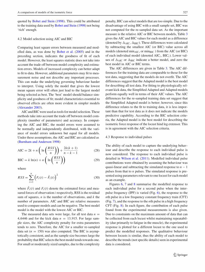
Table 3 Average AIC (�AIC = AICi −minAIC) and BIC (�BIC =BICi −minBIC) differences across 5 locusts for a whole data set and a re-sampleddata set
Model No. params. Whole data set Re-sampled data set Whole data set
�AICtrain-ingdata
�AICtestdata
�AICkickdata
�AICtrain-ingdata
�AICtestdata
�AICkickdata
�BICtrain-ingdata
�BICtestdata
�BICkickdata
Linear 4 89,800 131,000 35,200 128 422 365 89,800 131,000 194,000
Wiener 5 34,200 52,900 10,600 38.8 170 112 34,200 52,900 78,600
Cascade 7 34,600 65,600 19,600 78.8 214 214 43,600 65,600 97,500
Ding 6 15,000 46,500 20,200 79.6 30.1 5.65 15,000 46,524 69,153
Bobet and Stein 6 7,500 9,240 530 3.87 30.1 5.65 7,490 9,230 13,800
Simple adapted 5 8,380 7,140 200 0.00 21.1 0.01 8,370 7,130 10,600
Adapted 6 0.00 0.00 0.00 1.47 0.00 0.00 0.00 0.00 0.00
0 0.5 1 1.50
0.1
0.2
Nor
mal
ised
For
ce
(B)
0 0.1 0.2 0.3 0.4 0.50
0.1
0.2
Nor
mal
ised
For
ce
(C)
0 0.1 0.2 0.3 0.4 0.50
0.1
0.2
Nor
mal
ised
For
ce(D)
0 0.1 0.2 0.3 0.4 0.50
0.1
0.2
Nor
mal
ised
For
ce
(E)
0 0.1 0.2 0.3 0.4 0.50
0.1
0.2
Nor
mal
ised
For
ce
(F)
0 0.1 0.2 0.3 0.4 0.50
0.1
0.2
Time [s]
Nor
mal
ised
For
ce
(G)
0 0.1 0.2 0.3 0.4 0.50
0.1
0.2
Time [s]
Nor
mal
ised
For
ce
(H)
0 0.05 0.1 0.15 0.2 0.25 0.3
(A)
Nor
mal
ised
For
ce
Fig. 6 Comparison between a Experimental, and b–h modelledresponse to a second pulse for a range of IPFs, arrows indicate increas-ing IPF. The bold line gives the response to a single input. Modelled
responses are for b Linear model, c Wiener model, d Cascade model,e Ding model, f Bobet and Stein model, g Adapted Simplified model,h Adapted model
No model describes the response to a second pulse well(Fig. 6). This is partly due to the fact that training data did notcontain any two-pulse trains and so models were not trainedto describe the behaviour of a second pulse. Some models arebetter able to capture some of the underlying dynamics. Thelinear model, as expected, does not capture any of the non-lin-ear dynamics. The linear model performs the worst in termsof goodness of fit, due to this lack of ability to describe theunderlying non-linear behaviour. The Cascade and Wienermodels are able to describe the fact that the magnitude of
the second pulse is larger than that of the first. These mod-els do not, however, describe the change in pulse shape orthe variation in the response of a second pulse with IPF. Theunderlying behaviour described by the model of Ding et al.(2002) is very different to that found experimentally, suggest-ing that the model may not provide an accurate descriptionof the behaviour. As with the goodness of fit, AIC and BICfindings, the models of Bobet and Stein, Simplified Adaptedmodel and the Adapted model provide the best description ofthe behaviour. The early force depression is well predicted,
123
A comparison of models of the isometric force 529
0 0.5 1 1.5 2 2.5 30
0.1
0.2
(B)
Nor
mal
ised
For
ce
0 0.5 1 1.5 20
0.1
0.2
(C)
Nor
mal
ised
For
ce
0 0.5 1 1.5 20
0.1
0.2
(D)
Nor
mal
ised
For
ce
0 0.5 1 1.5 2 2.50
0.2
0.4
(E)
Nor
mal
ised
For
ce
0 0.5 1 1.5 20
0.1
0.2
(F)
Nor
mal
ised
For
ce
0 0.5 1 1.5 2 2.50
0.2
0.4
(G)
Time [s]
Nor
mal
ised
For
ce
0 0.5 1 1.5 2 2.50
0.2
0.4
(H)
Nor
mal
ised
For
ce
0.5 1 1.5 20
(A)
Nor
mal
ised
For
ce
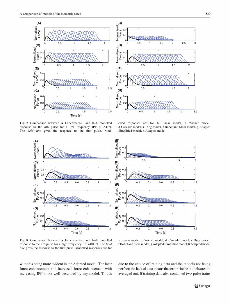
Fig. 7 Comparison between a Experimental, and b–h modelledresponse to the nth pulse for a low frequency IPF (12.5 Hz).The bold line gives the response to the first pulse. Mod-
elled responses are for b Linear model, c Wiener model,d Cascade model, e Ding model, f Bobet and Stein model, g AdaptedSimplified model, h Adapted model
0 0.5 1 1.5 20
0.1
0.2
(B)
Nor
mal
ised
For
ce
0 0.2 0.4 0.6 0.8 1 1.20
0.1
0.2
(C)
Nor
mal
ised
For
ce
0 0.2 0.4 0.6 0.8 1 1.20
0.1
0.2
(D)
Nor
mal
ised
For
ce
0 0.2 0.4 0.6 0.8 1 1.20
0.1
0.2
(E)
Nor
mal
ised
For
ce
0 0.2 0.4 0.6 0.8 1 1.20
0.1
0.2
(F)
Nor
mal
ised
For
ce
0 0.2 0.4 0.6 0.8 1 1.20
0.1
0.2
(G)
Time [s]
Nor
mal
ised
For
ce
0 0.2 0.4 0.6 0.8 1 1.20
0.1
0.2
(H)
Time [s]
Nor
mal
ised
For
ce
0 1
(A)
Nor
mal
ised
For
ce
Fig. 8 Comparison between a Experimental, and b–h modelledresponse to the nth pulse for a high frequency IPF (40 Hz). The boldline gives the response to the first pulse. Modelled responses are for
b Linear model, c Wiener model, d Cascade model, e Ding model,f Bobet and Stein model, g Adapted Simplified model, h Adapted model
with this being more evident in the Adapted model. The laterforce enhancement and increased force enhancement withincreasing IPF is not well described by any model. This is
due to the choice of training data and the models not beingperfect; the lack of data means that errors in the models are notaveraged out. If training data also contained two-pulse trains
123
530 E. Wilson et al.
then this behaviour could be described (Wilson 2011). How-ever, including two-pulse trains in the training data increaseits length and so the effects of fatigue are increased.
The response to the nth pulse in a low frequency CFT(Fig. 7) is reasonably well described by all models, with theexception of the linear model. The main discrepancy betweenthe modelled and measured data is that the modelled ampli-tude changes are less extreme than those seen in the measureddata.
From examination of the response of each pulse in ahigh frequency pulse train (Fig. 8), it is clear that again, asexpected, the linear model cannot describe the underlyingbehaviour. As with the response to the second pulse (Fig. 6),the model of Ding et al. (2002) describes the underlyingbehaviour poorly, again suggesting that the model does notprovide a good description of the behaviour of the locust hindleg extensor muscle. The other models capture the increaseand subsequent decrease in the pulse magnitude seen in theexperimental data. It is the inclusion of a non-linear saturationfunction that enables these models to capture this behaviour,and the fact that behaviour is frequency dependent.
Figures 6 and 8 show that the model of Ding et al. (2002)provides a poor model of the underlying behaviour. This isattributed to the relation Ri used by Ding et al. (2002) todescribe the non-linear summation of closely spaced pulses.The form of Ri (Eq. (12)) found using average model param-eters is not strongly influenced by the pulse separation, beingapproximately one for all IPFs. The model assumes that theforce enhancement always increases with IPF, but this is notthe case. For long pulse trains with high IPF, the magnitudesof the responses to later pulses are less than those for low IPFtrains. In other words, the force at the end of high IPF trainsis less enhanced than for low IPF trains. Since Ri cannotdescribe this behaviour, it is thought that the best solution isfor Ri not to depend significantly on the IPF. This influencesthe value of τc which is used as a time constant in other partsof the model.
4.4 Parameter sensitivity
A sensitivity analysis was carried out on the Adapted model.The Adapted model was chosen as the AIC and BIC calcu-lations indicated it was the best model. The next best modelaccording to AIC and BIC was the Simplified Adapted model.This model is equivalent to the Adapted model, with τ2 =0, and so a sensitivity analysis on the Adapted model alsoprovides some indication of the behaviour of the SimplifiedAdapted model.
A one-at-a-time approach was used, due to its concep-tual simplicity. This approach is similar to that used by Lawand Shields (2005) and provides a ‘local’ sensitivity esti-mate (Hamby 1994). Each parameter was varied in turn up to±10% of its nominal value. Corresponding average changes
in the force profile were measured by the force characteris-tics defined by Law and Shields (2005). These characteris-tics were: peak force (PF) defined as the maximum recordedforce, force-time integral (FTI), defined as the area under theforce trace, half relaxation time (HRT), defined as the timefor the force to decay from 90 to 50% of the peak force, laterelaxation time (LRT), defined as the time for the force todecay from 40 to 10% of peak force, relative fusion index(RFI), defined as the mean of the last four pulses’ minimadivided by their succeeding four peaks, and time to peak ten-sion (TPT), defined as the time required to reach 90% of thepeak force from time zero.
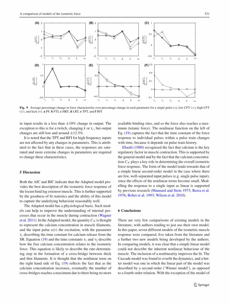
Initial parameter values were set to the average valuesgiven in Table 2. The model was stimulated by a single input,a low frequency pulse train, a high frequency pulse trainand a kick-type input so as to test the model behaviour undera range of conditions. Figure 9 gives the average ratio ofthe percentage change in each force characteristic as eachparameter is changed up to ±10% from its initial value.
The parameter A scales the force response. Percentagechanges in A result in equivalent percentage changes in thePF and FTI. Changing A has no effect on the force time mea-surements. The model is fitted to normalised data, with max-imum tetanic force equal to one. To apply the model to actualforce data, the parameter A would just change by the relevantscale factor, with all other being parameters being unchanged.Changes in the parameter k have the most effect on the PFand FTI. An increase in k causes a corresponding decrease inPF and FTI. Since the PF is affected, k also affects the TPT.Changes in k have a small effect on other force-time proper-ties. The parameter m changes all force characteristics a smallamount. For a twitch, increasing m decreases the PF and FTIa little, but for other inputs, the PF and FTI are increased.This is caused by the fact that m changes the specific shapeof the non-linearity. An increase in m decreases the value ofthe non-linear function for small inputs, yet increases it forhigh inputs. The parameter τc is the time constant associatedwith the low pass filtering of the input pulses (Eq. 20). Thetime constant τc is directly associated with the decay timeand so increases in τc cause increases in HRT and LRT. Thechange in decay time also affects the peak force and so τc hasan indirect influence on PF, TPT, FTI and RFI. The parameterτ1 is also a time constant, associated with force development.Increases in τ1 cause increases in HRT and LRT as expected.The time constant in turn affects the force magnitude andincreases in τ1 also result in increases in TPT, RFI (exceptfor high frequency inputs), PF, and FTI. The parameter τ2
has less influence on force characteristics. This is expectedas from Fig. 4 it is evident that the fit is changed little whenτ2 is not included in the model. The parameter τ2 has mostinfluence on force magnitude characteristics (PF, FTI).
The force response is not particularly sensitive to changesin any of the parameters. In most cases, a ±10% change
123
A comparison of models of the isometric force 531
(A) (B) (C)
(D) (E) (F)
Fig. 9 Average percentage change in force characteristic over percentage change in each parameter for a single pulse (◦), low CFT (×), high CFT(�), and kick (+). a PF, b FTI, c HRT, d LRT, e TPT, and f RFI
in input results in a less than ±10% change in output. Theexception to this is for a twitch, changing k or τc, but outputchanges are still low and around ±12.5%.
It is noted that the TPT and RFI for high frequency inputsare not affected by any changes in parameters. This is attrib-uted to the fact that in these cases, the responses are satu-rated and more extreme changes in parameters are requiredto change these characteristics.
5 Discussion
Both the AIC and BIC indicate that the Adapted model pro-vides the best description of the isometric force response ofthe locust hind leg extensor muscle. This is further supportedby the goodness of fit statistics and the ability of this modelto capture the underlying behaviour reasonably well.
The Adapted model has a physiological basis. Such mod-els can help to improve the understanding of internal pro-cesses that occur in the muscle during contraction (Wagneret al. 2011). In the Adapted model, the quantity CN is thoughtto represent the calcium concentration in muscle filaments,and the input pulse u(t) the excitation, with the parameterτc describing the time constant for calcium release from theSR. Equation (19) and the time constants τ1 and τ2 describehow the free calcium concentration relates to the isometricforce. This equation is likely to describe the rate-determin-ing step in the formation of a cross-bridge between thickand thin filaments. It is thought that the nonlinear term onthe right hand side of Eq. (19) reflects the fact that as thecalcium concentration increases, eventually the number ofcross-bridges reaches a maximum due to there being no more
available binding sites, and so the force also reaches a max-imum (tetanic force). The nonlinear function on the left ofEq. (19) captures the fact that the time constant of the forceresponse to individual pulses within a pulse train changeswith time, because it depends on pulse train history.
Ebashi (1980) recognised the fact that calcium is the keyregulatory factor in muscle contraction. This is supported bythe general model and by the fact that the calcium concentra-tion CN plays a key role in determining the overall isometricforce response. The form of the model tends towards that ofa simple linear second-order model in the case where thereare few, well-separated input pulses (e.g. single pulse input),since the effects of the nonlinear terms become small. Mod-elling the response to a single input as linear is supportedby previous research (Mannard and Stein 1973; Bawa et al.1976; Bobet et al. 1993; Wilson et al. 2010).
6 Conclusions
There are very few comparisons of existing models in theliterature, with authors tending to just use their own model.In this paper, seven different models of the isometric muscleresponse were compared, five taken from the literature anda further two new models being developed by the authors.In comparing models, it was clear that a simple linear modelcould not describe the inherent nonlinear behaviour of themuscle. The inclusion of a nonlinearity improves the fit. TheCascade model was found to overfit the dynamics, and a bet-ter model was one in which the linear part of the model wasdescribed by a second-order (‘Wiener model’), as opposedto a fourth order relation. With the exception of the model of
123
532 E. Wilson et al.
Ding et al. (2002), models of LNL structure further improvedthe fit. The model of Ding et al. (2002) performed worse thanthe Wiener model when describing the response to physio-logical kick data. It was also found that this model provided apoor description of the underlying behaviour. The best mod-els were Bobet and Stein’s model, the Adapted model and theSimplified Adapted model. The structures of these models,and hence their modelling capabilities, are similar.
The Adapted model was found to be the best model interms of goodness of fits, AIC and BIC. A parameter sen-sitivity analysis on this model found that the force responsewas not overly sensitive to parameter changes. The structureand model parameters of the Adapted model can be related tothe underlying physiological behaviour and the model high-lights the key role that calcium plays in muscle contraction.
Acknowledgments We are grateful to the BBSRC and EPSRC forsupport for this study.
References
Alexander RM (2003) Modelling approaches in biomechanics. PhilosTrans R Soc Lond B Biol Sci 358:1429–1435
Baratta R, Solomonow M (1990) The dynamic response model of ninedifferent skeletal muscles. IEEE Trans Biomed Eng 37(3):243–251
Bawa P, Mannard A, Stein RB (1976) Effects of elastic loads on thecontractions of cat muscles. Biol Cybern 22(3):129–137
Bobet J, Gossen ER, Stein RB (2005) A comparison of models of forceproduction during stimulated isometric ankle dorsiflexion in hu-mans. IEEE Trans Neural Syst Rehabil Eng 13(4):444–451
Bobet J, Stein RB (1998) A simple model of force generation by skel-etal muscle during dynamic isometric contractions. IEEE TransBiomed Eng 45(8):1010–1016
Bobet J, Stein RB, Oguztoreli MN (1993) A linear time—varyingmodel of force generation in skeletal muscle. IEEE Trans BiomedEng 40(10):1000–1006
Burnham KP, Anderson DR (1998) Model selection and multimodelinference a practical information—theoretical approach, 2nd edn.Springer, New York
Burrows M, Horridge GA (1974) The organization of inputs to moto-neurons of the locust metathoracic leg. Philos Trans R Soc LondB Biol Sci 269:49–94
Burrows M, Morris G (2001) The kinematics and neural control of high-speed kicking movements in the locust. J Exp Biol 204:3471–3481
Christophy M, Senan NAF, Lotz LC, O’Reilly OM (2011) Amusculoskeletal model for the lumbar spine. Biomech ModelMechanobiol (in Press)
Ding J, Wexler AS, Binder-Macleod SA (2002) A mathematical modelthat predicts the force-frequency relationship of human skeletalmuscle. Muscle Nerve 26(4):477–485
Ebashi S (1980) The croonian lecture, 1979: regulation of muscle con-traction. Proc R Soc Lond B Biol Sci 207:259–286
Freeman CT, Hughes A-M, Burridge JH, Chappell PH, Lewin PL, Rog-ers E (2009) A model of the upper extremity using fes for strokerehabilitation. J Biomech Eng 131(3):031011
Ghigliazza R, Holmes P (2005) Towards a neuromechanical model forinsect locomotion: hybrid dynamical systems. Regul Chaotic Dyn10(2):193–225
Hamby DM (1994) A reveiw of techniques for parameter sensitiv-ity analysis of environmental models. Environ Monitor Assess32:135–154
Hatze H (1977) A myocybernetic control model of skeletal muscle. BiolCybern 25(2):103–119
Heitler WJ (1988) The role of the fast extensor motor activity in thelocust kick reconsidered. J Exp Biol 136:289–309
Heitler WJ, Burrows M (1977) The locust jump. I. the motor pro-gramme. J Exp Biol 66:203–219
Hoyle G (1955) Neuromuscular mechanisms of a locust skeletal mus-cle. Proc R Soc Lond B Biol Sci 143:343–367
Hoyle G (1978) Distributions of nerve and muscle fibre types in locustjumping muscle. J Exp Biol 73:205–233
Huxley HE (1985) The crossbridge mechanism of muscular-contraction and its implications. J Exp Biol 115:17–30
Law LAF, Shields RK (2005) Mathematical models use varying param-eter strategies to represent paralyzed muscle force properties: asensitivity analysis. J NeuroEng Rehabil 2(12):18
Mannard A, Stein RB (1973) Determination of the frequency responseof isometric soleus muscle in the cat using random nerve stimula-tion. J Physiol 229:275–296
MathWorks T (2001) Curve fitting toolbox user’s guide. The Math-Works, Inc, Natick
Meijer K, Rosenthal M, Full RJ (2001) Muscle-like actuators? A com-parison between three electroactive polymers. Smart Struct Mater2001 Electroact Polym Actuators Devices 4329:7–15
Parmiggiani F, Stein RB (1981) Nonlinear summation of contractionsin cat muscles. ii. later facilitation and stiffness changes. J GenPhysiol 78:295–311
Repperger DA, Phillips CA, Neidhard-Doll A, Reynolds DB, BerlinJ (2006) Actuator design using biomimicry methods and a pneu-matic muscle system. Control Eng Pract 14:999–1009
Riener R, Quintern J (1997) A physiologically based model of muscleactivation verified by electrical stimulation. Bioelectrochem Bio-energ 43:257–264
Rosen J, Brand M, Fuchs M, Arcan M (2001) A myosignal-based pow-ered exoskeleton system. Syst Man Cybern Part A Syst Hum IEEETrans 31(3):210–222
Stein RB, Parmiggiani F (1981) Nonlinear summation of contractionsin cat muscles. i. early depression. J Gen Physiol 78(3):277–293
Theophilidis G, Burns MD (1983) The innervation of the mesothoracicflexor tibiae muscle of the locust. J Exp Biol 105:373–388
Valero-Cuevas FJ, Hoffmann H, Kurse MU, Kutch JJ, TheodorouEA (2009) Computational models for neuromuscular function.IEEE Rev Biomed Eng 2:110–135
Wagner H, Boström K, Rinke B (2011) Predicting isometric force frommuscular activation using a physiologically inspired model. Bio-mech Model Mechanobiol (in Press)
Wilson E (2011) Force response of locust skeletal muscle. Ph. D. thesis,Southampton University
Wilson E, Rustighi E, Mace BR, Newland PL (2010) Isometric forcegenerated by locust skeletal muscle: responses to single stimuli.Biol Cybern 6(102):503–511
Wilson E, Rustighi E, Mace BR, Newland PL (2011) Modelling the iso-metric force response to multiple pulse stimuli in locust skeletalmuscle. Biol Cybern (in Press)
Winters JM (1995) How detailed should muscle models be to under-stand multijoint movement coordination. Hum Mov Sci 14:401–442
123