Embed Size (px)
Citation preview

A COMPARISON OF PLOTTING FORMULAS 61
Jurnal Teknologi, 36(C) Jun. 2002: 61–74© Universiti Teknologi Malaysia
A COMPARISON OF PLOTTING FORMULAS FOR THEPEARSON TYPE III DISTRIBUTION
ANI SHABRI*
Abstract. Unbiased plotting position formulas are discussed to fit the Pearson Type 3 distribution(PIII). The best quantile estimate made from the plotting position should be unbiased and should havethe smallest root means square error among all such estimates. Probability plot correlation coefficient(PPCC) is used to evaluate goodness of fit to test the PIII distribution hypothesis. Results obtained usingthe annual maximum flow data from Peninsular of Malaysia based on PPCC show the plotting positionformulas consistently produced linear probability plots with correlation coefficient near to one. Basedon root mean square error (RMSE) and root mean absolute error, the Weibull formula performs betterthan the other formulas.
Keywords: Plotting Position, quantile, unbiased, root means square error
Abstrak. Formula kedudukan memplot tanpa bias dibincangkan untuk dipadankan dengan taburanPearson 3 (PIII). Penganggar kuantil kedudukan memplot terbaik seharusnya tanpa bias dan mempunyaimin punca ralat terkecil antara penganggar-penganggar yang lain. Pekali korelasi kedudukan memplotdigunakan sebagai ujian pemadanan cocokan untuk menguji hipotesis taburan PIII. Hasil keputusanmenggunakan data aliran maksimum daripada Semenanjung Malaysia berdasarkan ujian PPCCmenunjukkan rumus kedudukan memplot menghasilkan plot kebarangkalian yang linear denganpekali korelasi menghampiri satu. Berdasarkan punca min ralat kuasa dua dan punca min ralat mutlak,formula Weibull adalah terbaik antara formula-formula yang lain.
Kata Kunci Kedudukan Memplot, kuantil, tanpa bias, punca min ralat kuasa dua
1.0 INTRODUCTION
Probability plotting positions are used for the graphical display of annual maximumflood series and serve as estimates of the probability of exceedance of those series.Probability plots allow a visual examination of the adequacy of the fit provided byalternative parametric flood frequency models. They also provide a non-parametricmeans of forming an estimate of the data’s probability distribution by drawing a lineby hand and or automated means through the plotted points. Because of these attrac-tive characteristics, the graphical approach has been favoured by many hydrologistsand engineers. It has been widely used both in hydraulic engineering and water re-sources research [1, 3, 4 and 5].
* Jabatan Matematik, Fakulti Sains UTM Skudai, Johor, Malaysia, e-mail: [email protected],[email protected].
Untitled-83 02/16/2007, 18:3661

ANI SHABRI62
Probability plotting positions have been discussed by hydrologists and statisticiansfor many years. To date, more than ten plotting position formule have appeared in theliterature. Cunnane [2] and Stedinger et. al [7] published a very comprehensive reviewof the existing plotting formula. They postulated that a plotting formula should beunbiased and should have the smallest mean square error among all estimates.
Many distributions and various ways of fitting them are suitable. The selectiondistribution for any given flood records from among the alternative distributions isstill a subject of continuing investigations. In hydrology many distributions for floodfrequency analysis most often used, namely Extreme Value Type I (EV1), Generalextreme value (GEV), Pearson Type III (PIII), Log-Pearson Type III (LPIII), LogNormal (LNIII), General Pareto (GP), Wakeby and Weibull. Similarly, there are manyplotting formula available, several of which are summarized in Table 1.
The choice of plotting position formula for fit to the distributions has been dis-cussed many times in hydrology and statistical literature. Different plotting positionsattempt to use to achieve almost quantile-unbiasedness for different distributions. Inthis paper, the focus is to find the best plotting position formula to fit the PIII distribu-tion. In order to determine which plotting position formula is the most suitable for PIIIdistribution, the probability plot correlation coefficient test and RMSE and RMAEwere used. The parameters for each distribution was estimated using moment method.
2.0 PEARSON TYPE III DISTRIBUTION
The Pearson Type III (PIII) distribution is used widely by hydrologists for modelingflood flow frequencies [5] and [8]. The Pearson type III probability density functionmay be expressed as
( ) ( ) ( )( ) ( )− −= − −Γ
1α ξββ ξ β
αxf x x e (1)
where α, β and ξ are parameters. The parameters α, β and ξ are related to the firstthree moments of the random variable X as follows:
= + αµ ξβ (2)
=22
ασβ (3)
= 1/22βγ
β α (4)
3.0 THE INVERSE OF A PEARSON TYPE III DISTRIBUTION
The cumulative distribution function of PIII random variable is defined as
Untitled-83 02/16/2007, 18:3662

A COMPARISON OF PLOTTING FORMULAS 63
( ) ( )
( ) ( )∞
= >
= >
∫
∫
0
0
ξγ
γ
x
x
F x f x dx
F x f x dx (5)
which given the complex form of f (x) in (1), is not easily inverted. Many investiga-tions have developed approximation inversion formula. Stedinger [7] found the goodapproximation for inverse of standardized PIII random variable is
= +µ σi ip px K (6)
where ipK is referred to as frequency factor for the PIII distribution and can be written
as
= + − −
322 21
6 36
γ γγ γ
ii
pp
zK (7)
where µ, σ and γ are mean, standard deviation and skew coefficient respectively,
while ipz is the p th quantile of the zero-mean and unit-variance standard normal
distributions.
4.0 PLOTTING POSITION
Many investigators have advocated the use of quantile unbiased plotting positionswhen constructing probability plots. A quantile-unbiased plotting position is definedas [6]
( )= i ip F E X
where
[ ] ( )−= = …1 for 1,2, ,i iE X F p i n (8)
In situations where no historical floods are considered, most of them may be ex-pressed as a special case of general form
−=+ −1 2ii a
pn a
(9)
where pi is the plotting probability of the i th order statistic, n is the sample size and ais the plotting position parameter yielding approximately unbiased plotting positionsfor different distributions[1, 8]. For example, a = 0 for all distributions (Weibull for-mula), 0.44 for extreme value and exponential distribution (Gringorten formula), 0.5
Untitled-83 02/16/2007, 18:3663

ANI SHABRI64
for extreme value distribution (Hazen formula) and 3/8 for normal distribution (Blomformula)[7]. The approximation unbiased plotting position for PIII developed byNguyen et. al takes the form [8]
−=+ −
0.420.3 0.05γii
pn (10)
and is suitable for skews in the range − ≤ ≤3 3γ and samples in the range ≤ ≤5 100n .All of the plotting position formulas in this study are summarized in Table 1.
Table 1Table 1Table 1Table 1Table 1 Plotting Position Formulas (Cunnane, [2], Stedinger et al. [7])
ProponentProponentProponentProponentProponent FormulaFormulaFormulaFormulaFormula aaaaa Parent DistributionParent DistributionParent DistributionParent DistributionParent Distribution
Weibull (1939)i
n + 10 All distributions
Beard (1943)in−+0.31750.365
0.3175 All distributions
APLi
n− 0.35
~0.35 Used with Probability WeightedMoments Method (PWM)
Blom (1958)i
n
−+
3/8
1/4 0.375 Normal distributions
Cunnane (1977)in−+0.400.2
0.40 GEV and PIII distributions
Gringorten (1963)in
−+
0.440.12
0.44 Exponential, EV1 and GEVdistributions
Hazen (1914)i
n− 0.5
0.50 Extreme Value distributions
Nguyen et.al (1989)i
n γ−
+0.42
0.3 + 0.05 PIII distribution
5.0 PROBABILITY PLOT CORRELATION COEFFICIENT TEST
A probability plot is defined as a graphical representation of the i th order statistic ofthe sample, xi as a function of a plotting position. The i th order statistic is obtained byranking the observed sample from the smallest (i = 1) to the largest (i = n) value, thenxi equals the i th largest value.
A simple but powerful goodness-of-fit test is the probability plot correlation coeffi-cient (PPCC) test developed by Filliben in 1975, [7, 9]. The test uses the correlation rbetween the ordered observations and the corresponding fitted quantilies
( )ip
x F x−= 1 , determined by plotting position pi for each xi. The PPCC test is a
Untitled-83 02/16/2007, 18:3664
A COMPARISON OF PLOTTING FORMULAS 65
measure of linearity of a probability plot. If the sample to be tested is actually drawnfrom the hypothesized distribution, it is expected to be nearly linear and the correla-tion coefficient will be near to one. If x denotes the average value of the observationsand w denotes the average value of the fitted quantiles, the correlation coefficientsample can then be defined as
( )( )( ) ( )
i
i
i p
i p
x x x wr
x x x w
− −=
− −
∑
∑22 (11)
The 5% critical values of PPCC test statistic of the PIII distribution can be approxi-mated using
( )r n n γγ γ− = − ≤ 0.105 0.7482
0.05 exp 3.77 - 0.0290 0.000670 for 5 (12)
as given by Vogel et. al [8]. One rejects the hypothesized PIII distribution if theobserved value, r, is smaller than the critical value.
6.0 ROOT MEAN SQUARE ERROR AND ROOT MEANABSOLUTE ERROR
Root mean square errors (RMSE) and root mean absolute error (RMAE) are used tocompare the efficiency of the different plotting positions formulas. The RMSE is calcu-lated by the equation
in i p
ii
x xRMSE
n x=
− =
∑
1
1(13)
while RMAE is calculated by the equation
in i p
ii
x xRMAE
n x=
−= ∑
1
1(14)
where xi and ip
x are observed and quantile values, respectively for a given value of i.
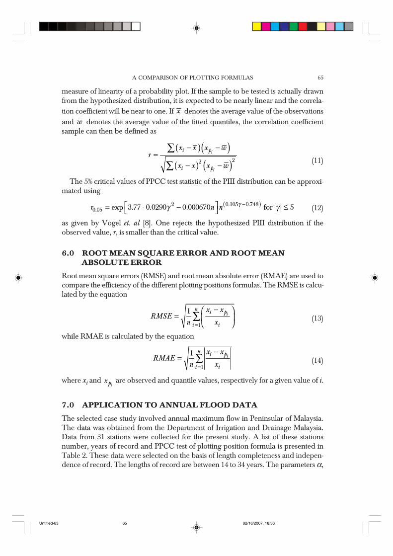
7.0 APPLICATION TO ANNUAL FLOOD DATA
The selected case study involved annual maximum flow in Peninsular of Malaysia.The data was obtained from the Department of Irrigation and Drainage Malaysia.Data from 31 stations were collected for the present study. A list of these stationsnumber, years of record and PPCC test of plotting position formula is presented inTable 2. These data were selected on the basis of length completeness and indepen-dence of record. The lengths of record are between 14 to 34 years. The parameters α,
Untitled-83 02/16/2007, 18:3665
ANI SHABRI66T
able
2C
orre
latio
n C
oeffi
cien
t Val
ue (r
) of
the
Plot
ting
Posi
tion
Form
ulas
and
5%
Cri
tical
Val
ue fo
r the
PII
I Dis
trib
utio
n
Sta
tio
nS
tati
on
Sta
tio
nS
tati
on
Sta
tio
nP
lott
ing
Po
siti
on
Fo
rmu
laP
lott
ing
Po
siti
on
Fo
rmu
laP
lott
ing
Po
siti
on
Fo
rmu
laP
lott
ing
Po
siti
on
Fo
rmu
laP
lott
ing
Po
siti
on
Fo
rmu
laN
um
ber
Nu
mb
erN
um
ber
Nu
mb
erN
um
ber
Sit
eS
ite
Sit
eS
ite
Sit
ennnn n
Wei
bu
llW
eib
ull
Wei
bu
llW
eib
ull
Wei
bu
llB
eard
Bea
rdB
eard
Bea
rdB
eard
AP
LA
PL
AP
LA
PL
AP
LB
lom
Blo
mB
lom
Blo
mB
lom
Cu
nn
ane
Cu
nn
ane
Cu
nn
ane
Cu
nn
ane
Cu
nn
ane
Gri
ngo
rten
Gri
ngo
rten
Gri
ngo
rten
Gri
ngo
rten
Gri
ngo
rten
Haz
enH
azen
Haz
enH
azen
Haz
enN
guye
nN
guye
nN
guye
nN
guye
nN
guye
n5%
Cri
tica
l V
alu
e5%
Cri
tica
l V
alu
e5%
Cri
tica
l V
alu
e5%
Cri
tica
l V
alu
e5%
Cri
tica
l V
alu
e17
3240
11
160.
981
0.97
90.
975
0.97
80.
978
0.97
70.
976
0.97
70.
941
1737
451
232
0.98
30.
984
0.98
40.
984
0.98
40.
984
0.98
40.
983
0.95
618
3640
23
180.
985
0.98
80.
992
0.98
90.
989
0.98
90.
990
0.98
60.
936
2130
422
421
0.98
20.
985
0.98
70.
986
0.98
60.
986
0.98
70.
986
0.95
222
3540
15
180.
970
0.97
30.
978
0.97
40.
974
0.97
50.
975
0.97
00.
934
2237
471
634
0.87
2*0.
890*
0.93
10.
893*
0.89
5*0.
898*
0.90
2*0.
777*
0.91
125
2741
17
220.
965
0.97
10.
978
0.97
20.
972
0.97
30.
975
0.96
70.
940
2928
401
815
0.93
40.
947
0.96
50.
949
0.95
10.
953
0.95
60.
931
0.91
330
3040
19
160.
987
0.98
80.
987
0.98
80.
988
0.98
80.
988
0.98
80.
951
3224
433
1021
0.98
30.
987
0.99
20.
988
0.98
80.
989
0.99
00.
985
0.94
133
2940
111
140.
980
0.97
90.
979
0.97
80.
978
0.97
80.
977
0.97
80.
937
3519
426
1229
0.99
20.
993
0.99
40.
993
0.99
30.
993
0.99
40.
993
0.95
736
2940
313
230.
955
0.95
1*0.
944*
0.94
9*0.
949*
0.94
8*0.
946*
0.94
8*0.
955
4019
462
1434
0.96
30.
971
0.98
20.
973
0.97
40.
975
0.97
70.
960
0.94
140
2341
215
260.
982
0.98
10.
981
0.98
10.
981
0.98
10.
980
0.98
10.
959
4121
413
1621
0.98
60.
983
0.97
90.
982
0.98
10.
981
0.98
00.
980
0.95
941
3145
317
140.
920
0.93
90.
965
0.94
30.
945
0.94
80.
953
0.90
90.
901
4218
416
1815
0.97
50.
978
0.98
10.
979
0.98
00.
980
0.98
10.
980
0.94
342
1941
519
160.
984
0.98
80.
992
0.98
80.
989
0.98
90.
990
0.98
70.
936
4223
450
2019
0.97
00.
976
0.98
30.
977
0.97
70.
978
0.97
90.
971
0.93
342
3245
221
190.
987
0.98
70.
988
0.98
70.
987
0.98
70.
987
0.98
70.
953
4732
461
2216
0.98
20.
982
0.98
30.
982
0.98
20.
982
0.98
20.
982
0.94
248
3244
123
250.
916*
0.93
40.
956
0.93
70.
939
0.94
20.
956
0.89
9*0.
920
5129
437
2418
0.98
40.
987
0.99
00.
987
0.98
70.
988
0.98
80.
985
0.93
851
3043
225
320.
962
0.96
70.
970
0.96
80.
968
0.96
90.
969
0.96
10.
943
5229
436
2615
0.98
80.
987
0.98
50.
986
0.98
60.
986
0.98
50.
986
0.93
853
2044
327
230.
970
0.97
70.
985
0.97
90.
979
0.98
00.
982
0.96
90.
935
5428
401
2818
0.98
70.
988
0.98
90.
988
0.98
80.
988
0.98
80.
987
0.94
157
2144
229
370.
985
0.98
90.
992
0.99
00.
990
0.99
00.
991
0.98
50.
954
5724
411
3020
0.80
5*0.
834*
0.88
0*0.
841*
0.84
4*0.
848*
0.85
4*0.
761*
0.90
260
1941
131
310.
986
0.98
70.
987
0.98
70.
987
0.98
70.
987
0.98
70.
965
* T
he h
ypot
hese
s of p
lotti
ng p
ositi
on fo
rmul
a is
reje
cted
at 5
% si
gnifi
cant
leve
l.
Untitled-83 02/16/2007, 18:3666

A COMPARISON OF PLOTTING FORMULAS 67
Figure 1 Comparison of Observed and Computed Frequency Curves For The 4 Stations WithDifference r
(a) Station number 12, For r > 0.991 (b) Station number 6, With 0.776 < r < 0.932
(c) Station number 23 With 0.898 < r < 0.957 (d) Station number 30 With o.760 < r < 0.888
Untitled-83 02/16/2007, 18:3767

ANI SHABRI68
β and ξ of the Pearson Type 3 distribution were estimated by using the method ofmoment.
Two criteria were used for comparing the eight plotting positions. The first criterionis defined as the probability plot goodness of fit. Table 2 shows the probability plotcorrelation coefficient, r, for 8 plotting position formulas and the 5% critical value of thePPCC test statistic using equation (11).
The correlation coefficient values of the plotting position formulas for each stationscorresponding with 5% critical values are shown in Figure 1. Table 2 and Figure 1show that the all plotting position formulas fall in accepted region at 5% critical valuesat all stations except the APL is rejected at two stations, Nguyen is rejected at fourstations and the other formulas are rejected at three stations.
Two sets of observed data were selected for numerical demonstration. Figure 3 andFigure 4 show a demonstration comparison of plotting position formulas for r areaccepted for station 12 and rejected for station 30 at 5% critical values. From Figure 3,it can seen that plots based on all of plotting position formulas are closed to data.However Figure 4 shows that the PIII using these plotting position formulas do notshow good fit to the data especially at the largest data.
0.75
0.8
0.85
0.9
0.95
1
1.05
1 2 3 4 5 6 7 8 9 10 11 12 13 14 15 16 17 18 19 20 21 22 23 24 25 26 27 28 29 30 31 32
Station
Cor
rela
tion
Coe
ffici
ent,
r
Weibull Beard APL Blom Cunnane Gringorten Hazen Critical Nguyen
Rejection Regions
Acception Regions
5% Critical Values
Figure 3 The Probability Plot Correlation Coefficient for the 8 Plotting Position Formulas and 5%Critical Values
The second criterion is the defined as the RMSE and RMAE. Table 3 and 4 list thevalues of RMSE and RMAE for PIII by using the plotting position formulas.
Untitled-83 02/16/2007, 18:3768

A COMPARISON OF PLOTTING FORMULAS 69
Tab
le 3
Val
ues o
f Roo
t Mea
ns S
quar
e E
rror
Plo
ttin
g P
osit
ion
For
mu
laSt
atio
nW
eib
ull
Bea
rdA
PL
Blo
mC
un
nan
eG
rin
gort
enH
azen
Ngu
yen
10.
153
0.17
50.
182
0.18
30.
187
0.19
40.
205
0.19
02
0.19
00.
211
0.21
40.
215
0.21
80.
221
0.22
70.
220
30.
100
0.11
50.
117
0.12
00.
122
0.12
60.
132
0.12
64
0.17
10.
126
0.12
30.
117
0.11
30.
107
0.09
70.
110
50.
271
0.31
70.
324
0.32
70.
332
0.34
00.
352
0.33
76
7.01
18.
796
8.99
39.
247
9.46
09.
828
10.4
529.
884
77.
011
8.79
68.
993
9.24
79.
460
9.82
810
.452
9.88
48
0.09
20.
088
0.08
90.
088
0.08
80.
087
0.08
70.
096
90.
169
0.11
00.
110
0.10
30.
100
0.09
80.
100
0.10
110
0.07
50.
079
0.08
00.
084
0.08
60.
090
0.09
80.
092
110.
126
0.13
10.
136
0.13
50.
137
0.14
10.
147
0.13
912
0.10
90.
115
0.11
70.
118
0.11
90.
122
0.12
70.
121
130.
358
0.43
60.
448
0.45
50.
463
0.47
80.
501
0.47
014
0.11
50.
113
0.11
20.
113
0.11
30.
113
0.11
20.
118
150.
199
0.23
80.
244
0.24
80.
253
0.26
10.
275
0.25
716
0.00
50.
005
0.00
60.
005
0.00
50.
005
0.00
50.
005
170.
754
0.77
80.
785
0.78
20.
784
0.78
70.
791
0.79
318
0.09
70.
070
0.07
00.
066
0.06
40.
061
0.05
70.
062
190.
005
0.00
40.
003
0.00
40.
004
0.00
30.
003
0.00
420
1.10
61.
250
1.26
31.
280
1.29
31.
315
1.34
91.
309
210.
134
0.12
50.
131
0.13
20.
136
0.14
40.
160
0.14
022
0.16
90.
174
0.18
00.
181
0.18
50.
192
0.20
60.
189
235.
071
5.18
45.
216
5.21
85.
235
5.26
65.
322
5.23
124
0.25
30.
321
0.33
10.
343
0.35
30.
372
0.40
20.
365
250.
336
0.35
60.
359
0.35
90.
361
0.36
30.
367
0.36
326
0.13
30.
183
0.19
30.
205
0.21
60.
234
0.26
60.
225
270.
120
0.11
90.
120
0.11
90.
120
0.12
00.
121
0.12
628
0.18
90.
591
0.64
40.
740
0.80
90.
923
1.10
80.
876
290.
252
0.27
40.
276
0.27
80.
280
0.28
40.
289
0.28
430
2.46
63.
061
3.18
23.
226
3.30
63.
447
3.69
23.
399
310.
141
0.12
10.
121
0.12
00.
119
0.11
90.
121
0.11
9
Untitled-83 02/16/2007, 18:3769

ANI SHABRI70T
able
4V
alue
s of R
oot M
eans
Abs
olut
e E
rror
P
lott
ing
Pos
itio
n F
orm
ula
Stat
ion
Wei
bu
llB
eard
AP
LB
lom
Cu
nn
ane
Gri
ngo
rten
Haz
enN
guye
n1
0.33
40.
336
0.34
20.
338
0.33
90.
341
0.34
80.
342
0.35
90.
363
0.36
80.
364
0.36
40.
365
0.36
70.
366
30.
294
0.29
90.
297
0.3
0.30
10.
301
0.30
30.
305
40.
280.
262
0.25
40.
258
0.25
60.
254
0.24
90.
255
50.
450.
463
0.46
20.
466
0.46
70.
469
0.47
20.
475
61.
849
1.96
91.
986
1.99
62.
009
2.03
2.06
52.
022
70.
239
0.23
50.
234
0.23
50.
235
0.23
40.
233
0.23
48
0.27
40.
274
0.27
10.
274
0.27
40.
274
0.27
40.
276
90.
321
0.27
30.
271
0.26
20.
256
0.25
80.
265
0.25
510
0.24
0.25
60.
253
0.26
10.
263
0.26
60.
272
0.26
911
0.31
50.
309
0.31
90.
309
0.31
0.31
20.
316
0.31
112
0.26
30.
266
0.26
10.
267
0.26
70.
268
0.26
90.
271
130.
514
0.53
20.
540.
536
0.53
80.
542
0.54
80.
5414
0.23
80.
240.
238
0.24
0.24
10.
241
0.24
10.
248
150.
373
0.38
60.
388
0.38
90.
391
0.39
40.
398
0.39
216
0.06
40.
063
0.06
50.
063
0.06
30.
063
0.06
40.
064
170.
715
0.73
60.
751
0.73
90.
741
0.74
30.
747
0.72
418
0.25
50.
235
0.23
30.
230.
228
0.22
40.
217
0.22
619
0.06
0.05
40.
051
0.05
30.
053
0.05
30.
052
0.05
520
0.79
20.
821
0.81
90.
826
0.82
90.
833
0.83
90.
835
210.
311
0.30
70.
307
0.31
0.31
10.
313
0.31
70.
312
220.
337
0.34
50.
351
0.34
70.
348
0.35
0.35
30.
349
231.
801
1.81
81.
829
1.82
31.
825
1.82
81.
834
1.81
124
0.40
90.
417
0.41
60.
419
0.42
0.42
20.
426
0.42
225
0.47
0.47
80.
488
0.48
0.48
0.48
10.
484
0.48
260.
326
0.36
60.
373
0.37
50.
380.
388
0.40
20.
384
270.
316
0.32
0.31
90.
321
0.32
10.
321
0.32
10.
3228
0.37
0.49
0.50
40.
525
0.54
10.
565
0.60
40.
557
290.
423
0.43
0.42
90.
432
0.43
20.
433
0.43
40.
435
301.
297
1.37
51.
401
1.39
51.
404
1.41
91.
445
1.37
631
0.29
40.
282
0.28
10.
282
0.28
30.
283
0.28
40.
282
Untitled-83 02/16/2007, 18:3770

A COMPARISON OF PLOTTING FORMULAS 71
The eight plotting position formulas were ranked for all stations according to thevalues of RMSE and RMAE on scale 1 to 8, with one being the best method.
0100200300400500
600700
-2 -1 0 1 2 3 4 5
Frequency Factors
Dis
char
ge, m
3/s
Data Weibull Beard APL BlomCunnane Gringorten Hazen Nguyen
-2000
0
2000
4000
6000
8000
10000
12000
14000
16000
-1 -0.5 0 0.5 1 1.5 2 2.5
Frequency Factors
Dis
char
ge, m
3/s
Data Weibull Beard APL BlomCunnane Gringorten Hazen Nguyen
Figure 4 Comparison of Observed and Quantile Using The Plotting Position Formulas (r AreAccepted At 5% Critical Values, Station 12)
Figure 5 Comparison of Observed and Quantile Using The Plotting Position Formulas (r AreRejected At 5% Critical Values, Station 30)
Table 5 ranks the eight plotting position formulas according to RMSE. It can seenthat the Weibull formula was the best, followed by APL, Beard, Blom, Cunnane,Gringorten, Nguyen and Hazen formulas in descending order of their performance.
The ranking of the eight plotting position formulas according to RMAE is given inTable 6. Clearly Weibull formula was the best of all, followed by APL, Beard, Blom,
Untitled-83 02/16/2007, 18:3771

ANI SHABRI72
Cunnane, Gringorten, Hazen and Nguyen formulas in descending order of their per-formance. Again, the previous conclusions hold. However those differences betweenplotting positions were not too great and therefore these plotting positions could beconsidered comparable for practical purpose.
Table 5 Ranking of the Plotting Position Formulas for 31 Stations by Root Means Square Error(RMSE) on a scale of 1 to 8 with 1 being the best method
PlottingPosition Number of Stations Receiving Ranking
1 2 3 4 5 6 7 8
Weibull 13 0 0 0 0 3 6 8
Beard 3 13 3 1 0 8 3 0
APL 10 3 7 3 2 3 2 1
Blom 2 2 8 9 10 0 0 0
Cunnane 2 0 4 15 10 0 0 0
Gringorten 0 6 6 0 5 8 4 1
Hazen 4 5 2 0 3 4 5 9
Nguyen 2 2 3 2 2 5 7 7
Table 6 Ranking of the Plotting Position Formulas for 31 Stations by Root Means Absolute Error(RMAE) on a scale of 1 to 8 with 1 being the best method
PlottingPosition Number of Stations Receiving Ranking
1 2 3 4 5 6 7 8
Weibull 20 2 0 1 1 1 0 6
Beard 1 13 12 0 0 0 5 0
APL 5 9 4 1 2 2 3 5
Blom 1 1 8 16 3 2 0 0
Cunnane 0 1 2 8 18 2 0 0
Gringorten 0 1 3 1 3 15 8 0
Hazen 3 1 0 0 1 1 11 14
Nguyen 1 3 2 4 3 8 4 6
Untitled-83 02/16/2007, 18:3772

A COMPARISON OF PLOTTING FORMULAS 73
8.0 CONCLUSIONS
Probability plots and the probability-plot correlation coefficient test statistic are usedfor testing the PIII using plotting position formula to fit annual maximum flow data.The PPCC test statistic was found to be a useful tool for discriminating among com-peting probability and plotting position formula. Eight plotting position formulas werecompared for their ability to fit flood flow data. Overall these plotting position formu-las consistently produced linear probability plots with r nearly one as measured by thePPCC test statistics. If an unbiased plotting position formula is required for the PIIIdistribution, then the Weibull formula would be the best selection.
REFERENCES[1] Adamowski, K. 1981. Plotting Formula For Flood Frequency, Water Resour. Bulletin, 17(2): 197-202.[2] C. Cunnane, C. 1978. Unbiased Plotting Positions- A Review, Journal of Hydrology. 37: 205-222.[3] Guo, S. L. 1990. A Discussion On Unbiased Plotting Positions For The General Extreme Value Distribution,
Journal of Hydrology. 121: 33-44.[4] Guo, S. L. 1990. Unbiased Plotting Position Formula For Historical Floods, Journal of Hydrology. 121: 45-61.[5] Ji Xuewu, Ding Jing, H. W. Shen, and J. D.Salas. 1984. Plotting Positions For Pearson, Journal of Hydrology.
74: 1-29.[6] Kottegoda N. T., and R. Rosso. 1997. Probability, Statistics, and Reliability for Civil and Environmental
Engineers. Mc-Graw Hill Book Co., New York.[7] Stedinger, J. R., R. M. Vogel, and G. E. Foufoula. 1993. Frequency Analysis of Extreme Events. Handbook
of Applied Hydrology. Mc-Graw Hill Book Co., New York, Chapter 18.[8] Vogel, R. M., and D. M. McMartin. 1991. Probability Plot Goodness-of-Fit and Skweness Estimation
Procedures for the Pearson Type 3 Distribution, Water Resour. Res., 27(12): 3149-3158.[9] Vogel, R. M. 1986. The Probability Plot Correlation Coefficient Test for the Normal, Lognormal, and
Gumbel Distribution Hypotheses, Water Resour. Res., 22(4): 587-590.
Untitled-83 02/16/2007, 18:3773