A Comparison of Surface Layer and Surface Turbulent Flux

VOLUME 32 FEBRUARY 2002J O U R N A L O F P H Y S I C A L O C E A N O G R A P H Y

q 2002 American Meteorological Society 383

A Comparison of Surface Layer and Surface Turbulent Flux Observations over theLabrador Sea with ECMWF Analyses and NCEP Reanalyses

IAN A. RENFREW

British Antarctic Survey, Cambridge, United Kingdom

G. W. K. MOORE

Department of Physics, University of Toronto, Toronto, Ontario, Canada

PETER S. GUEST

Naval Postgraduate School, Monterey, California

KARL BUMKE

Institut fur Meereskunde, Universitat Kiel, Kiel, Germany

(Manuscript received 17 December 1999, in final form 4 August 2000)

ABSTRACT

Comparisons are made between a time series of meteorological surface layer observational data taken onboard the R/V Knorr, and model analysis data from the European Centre for Medium-Range Weather Forecasting(ECMWF) and the National Centers for Environmental Prediction (NCEP). The observational data were gatheredduring a winter cruise of the R/V Knorr, from 6 February to 13 March 1997, as part of the Labrador Sea DeepConvection Experiment. The surface layer observations generally compare well with both model representationsof the wintertime atmosphere. The biases that exist are mainly related to discrepancies in the sea surfacetemperature or the relative humidity of the analyses.

The surface layer observations are used to generate bulk estimates of the surface momentum flux, and thesurface sensible and latent heat fluxes. These are then compared with the model-generated turbulent surfacefluxes. The ECMWF surface sensible and latent heat flux time series compare reasonably well, with overestimatesof only 13% and 10%, respectively. In contrast, the NCEP model overestimates the bulk fluxes by 51% and27%, respectively. The differences between the bulk estimates and those of the two models are due to differentsurface heat flux algorithms. It is shown that the roughness length formula used in the NCEP reanalysis projectis inappropriate for moderate to high wind speeds. Its failings are acute for situations of large air–sea temperaturedifference and high wind speed, that is, for areas of high sensible heat fluxes such as the Labrador Sea, theNorwegian Sea, the Gulf Stream, and the Kuroshio. The new operational NCEP bulk algorithm is found to bemore appropriate for such areas.

It is concluded that surface turbulent flux fields from the ECMWF are within the bounds of observationaluncertainty and therefore suitable for driving ocean models. This is in contrast to the surface flux fields fromthe NCEP reanalysis project, where the application of a more suitable algorithm to the model surface-layermeteorological data is recommended.

1. Introduction

Deep convection in the ocean is a key component ofthe thermohaline circulation, governing both the loca-tion and timescale of vertical mixing processes at highlatitudes. The occurrence of deep convection is a mul-tistage process, requiring as a first step that the oceanbe preconditioned into a state of neutral stratification.

Corresponding author address: Ian Renfrew, British Antarctic Sur-vey, High Cross, Madingley Road, Cambridge CB3 0ET, United King-dom.E-mail: [email protected]

For the open ocean, this occurs through the tilting ofisopycnals to maintain thermal wind balance in the pres-ence of a boundary current or through topographic forc-ing, either of which must be combined with cooling andevaporation into the lower atmosphere. In the secondstep, further losses of heat and moisture by the surfacewaters lead to a destabilization of the water column andthe triggering of convective plumes within the precon-ditioned region. The third step is the sinking and spread-ing of the modified water mass and an eventual shut-down of convection (e.g., Killworth 1983; Marshall andSchott 1999). Deep convection in the open ocean is a

384 VOLUME 32J O U R N A L O F P H Y S I C A L O C E A N O G R A P H Y

FIG. 1. The track of the R/V Knorr during the Feb and Mar 1997Labrador Sea Experiment cruise. Overlain as a dashed line is the icecover used by the NCEP model from 18 Feb 1997.

process that is difficult to observe, due to its localizedoccurrence and rapid timescale, yet plays a crucial rolein the thermohaline circulation and hence the climatesystem. To redress this situation a major internationalproject has been initiated: The Labrador Sea Deep Con-vection Experiment (Lab Sea Group 1998). Its aim is‘‘improving our understanding of the convective processin the ocean and its representation in models,’’ throughoceanographic and meteorological observations, theory,and modeling. The Labrador Sea was chosen due to itsrelative proximity to North America, compared to theother major convection sites of the Greenland–Iceland–Norwegian seas and the Weddell Sea. The choice wasmade additionally interesting by the somewhat ephem-eral nature of Labrador Sea convection; there is evidencefor significant decadal variability in the amount of con-vection that takes place (Dickson et al. 1996). Indeedit is the one region where convection shut down in a‘‘realistic’’ coupled atmosphere–ocean climate model-ing study carried out recently (Wood et al. 1999).

Modeling the ocean circulation in a realistic way re-lies on the faithful representation of atmosphere–oceaninteractions. To be precise, the fluxes of momentum,heat, and moisture between the atmosphere and oceanmust be accurate. Nowhere is this more critical than inconvectively active regions where, as discussed above,the atmosphere directly forces the ocean dynamics. Togenerate accurate atmosphere–ocean fluxes requires firstthat the atmospheric boundary layer is realistic and sec-ond that the derivation of surface fluxes is carried outusing a suitable model formulation. In this study weaddress these two requirements in turn. First, a timeseries of observations from a cruise of the R/V Knorrin the Labrador Sea during February and March 1997is compared to model analyses data. The analyses arethe operational analyses from the European Centre forMedium-Range Weather Forecasts (ECMWF), and thereanalyses from the National Centers for EnvironmentalPrediction (NCEP)–National Center for AtmosphericResearch (NCAR) project. These are two of the leadingnumerical weather prediction centers in the world andtwo of the most common choices for providing surfaceflux fields to drive ocean models. In section 2 the ob-servational and model data are described in detail. Sec-tion 3 details a surface layer meteorological data com-parison, and following this, section 4 details a surfaceturbulent flux comparison. The differences in the surfaceheat flux fields warrant an explanation, and this leadsto an investigation of surface flux algorithms in section5. Conclusions are drawn in section 6.

2. Datasets

a. Observational data

A 40-day cruise in the Labrador Sea, from 6 Februaryto 13 March 1997, was undertaken by the R/V Knorras part of the field component of the Labrador Sea Ex-

periment (Fig. 1). In companion to the comprehensiveoceanographic field work that took place (e.g., Lab SeaGroup 1998), a number of meteorological experimentswere on board the Knorr. For example, a group fromthe Bedford Institute of Oceanography carried out tur-bulent heat and moisture flux measurements, and agroup from the University of Kiel carried out turbulentheat flux and precipitation measurements (Bumke et al.2002; 2001, manuscript submitted to J. Phys. Ocean-ogr.). In addition, a team of scientists released rawin-sondes, typically every 6 hours and occasionally every3 hours, and these data were transmitted via the GlobalTelecommunications System (GTS) to national forecastcenters.

Throughout the cruise standard meteorological vari-ables were automatically logged by the ship’s ImprovedMeteorological (IMET) measurement system. Theseform the main dataset used in this study. Temperature,humidity, pressure, and wind velocity were measuredusing a thermistor, hygrometer, barometer, and propelleranemometer located on the foremast approximately 19.5m above the sea surface. The ship’s motion, as deter-mined by a GPS navigation system, was subtracted fromthe anemometer-measured wind vector to obtain a truewind vector. Usually the ship was steaming betweenstations or performing oceanographic CTD measure-ments. In either case, the wind was usually from thebow and the ship’s velocity vector was constant. Basedon sensor comparisons and a numerical wind tunnel test(Moat and Yelland 1998) we estimate that when the

FEBRUARY 2002 385R E N F R E W E T A L .

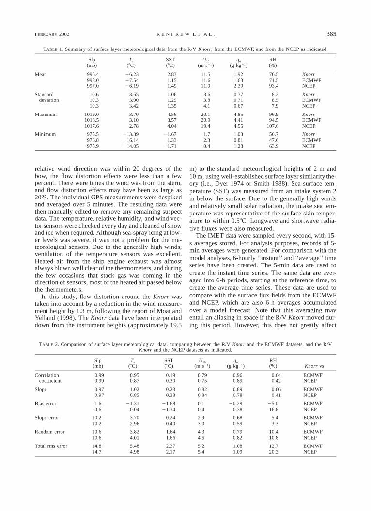
TABLE 1. Summary of surface layer meteorological data from the R/V Knorr, from the ECMWF, and from the NCEP as indicated.

Slp(mb)

Ta

(8C)SST(8C)

U10

(m s21)qa

(g kg21)RH(%)

Mean 996.4998.0997.0

26.2327.5426.19

2.831.151.49

11.511.611.9

1.921.632.30

76.571.593.4

KnorrECMWFNCEP

Standarddeviation

10.610.310.3

3.653.903.42

1.061.291.35

3.63.84.1

0.770.710.67

8.28.57.9

KnorrECMWFNCEP

Maximum 1019.01018.51017.6

3.703.102.78

4.563.574.04

20.120.919.4

4.854.414.55

96.994.5

107.6

KnorrECMWFNCEP

Minimum 975.5976.8975.9

213.39216.14214.05

21.6721.3321.71

1.72.30.4

1.030.811.28

56.747.663.9

KnorrECMWFNCEP

TABLE 2. Comparison of surface layer meteorological data, comparing between the R/V Knorr and the ECMWF datasets, and the R/VKnorr and the NCEP datasets as indicated.

Slp(mb)

Ta

(8C)SST(8C)

U10

(m s21)qa

(g kg21)RH(%) Knorr vs

Correlationcoefficient

0.990.99

0.950.87

0.190.30

0.790.75

0.960.89

0.640.42

ECMWFNCEP

Slope 0.970.97

1.020.85

0.230.38

0.820.84

0.890.78

0.660.41

ECMWFNCEP

Bias error 1.60.6

21.310.04

21.6821.34

0.10.4

20.290.38

25.016.8

ECMWFNCEP

Slope error 10.210.2

3.702.96

0.240.40

2.93.0

0.680.59

5.43.3

ECMWFNCEP

Random error 10.610.6

3.824.01

1.641.66

4.34.5

0.790.82

10.410.8

ECMWFNCEP

Total rms error 14.814.7

5.484.98

2.372.17

5.25.4

1.081.09

12.720.3

ECMWFNCEP

relative wind direction was within 20 degrees of thebow, the flow distortion effects were less than a fewpercent. There were times the wind was from the stern,and flow distortion effects may have been as large as20%. The individual GPS measurements were despikedand averaged over 5 minutes. The resulting data werethen manually edited to remove any remaining suspectdata. The temperature, relative humidity, and wind vec-tor sensors were checked every day and cleaned of snowand ice when required. Although sea-spray icing at low-er levels was severe, it was not a problem for the me-teorological sensors. Due to the generally high winds,ventilation of the temperature sensors was excellent.Heated air from the ship engine exhaust was almostalways blown well clear of the thermometers, and duringthe few occasions that stack gas was coming in thedirection of sensors, most of the heated air passed belowthe thermometers.

In this study, flow distortion around the Knorr wastaken into account by a reduction in the wind measure-ment height by 1.3 m, following the report of Moat andYelland (1998). The Knorr data have been interpolateddown from the instrument heights (approximately 19.5

m) to the standard meteorological heights of 2 m and10 m, using well-established surface layer similarity the-ory (i.e., Dyer 1974 or Smith 1988). Sea surface tem-perature (SST) was measured from an intake system 2m below the surface. Due to the generally high windsand relatively small solar radiation, the intake sea tem-perature was representative of the surface skin temper-ature to within 0.58C. Longwave and shortwave radia-tive fluxes were also measured.

The IMET data were sampled every second, with 15-s averages stored. For analysis purposes, records of 5-min averages were generated. For comparison with themodel analyses, 6-hourly ‘‘instant’’ and ‘‘average’’ timeseries have been created. The 5-min data are used tocreate the instant time series. The same data are aver-aged into 6-h periods, starting at the reference time, tocreate the average time series. These data are used tocompare with the surface flux fields from the ECMWFand NCEP, which are also 6-h averages accumulatedover a model forecast. Note that this averaging mayentail an aliasing in space if the R/V Knorr moved dur-ing this period. However, this does not greatly affect


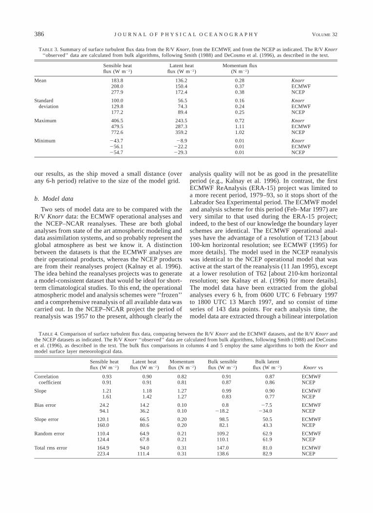
TABLE 3. Summary of surface turbulent flux data from the R/V Knorr, from the ECMWF, and from the NCEP as indicated. The R/V Knorr‘‘observed’’ data are calculated from bulk algorithms, following Smith (1988) and DeCosmo et al. (1996), as described in the text.

Sensible heatflux (W m22)

Latent heatflux (W m22)

Momentum flux(N m22)

Mean 183.8208.0277.9

136.2150.4172.4

0.280.370.38

KnorrECMWFNCEP

Standarddeviation

100.0129.8177.2

56.574.389.4

0.160.240.25

KnorrECMWFNCEP

Maximum 406.5479.5772.6

243.5287.3359.2

0.721.111.02

KnorrECMWFNCEP

Minimum 243.7256.1254.7

28.9222.2229.3

0.010.010.01

KnorrECMWFNCEP

TABLE 4. Comparison of surface turbulent flux data, comparing between the R/V Knorr and the ECMWF datasets, and the R/V Knorr andthe NCEP datasets as indicated. The R/V Knorr ‘‘observed’’ data are calculated from bulk algorithms, following Smith (1988) and DeCosmoet al. (1996), as described in the text. The bulk flux comparisons in columns 4 and 5 employ the same algorithms to both the Knorr andmodel surface layer meteorological data.

Sensible heatflux (W m22)

Latent heatflux (W m22)

Momentumflux (N m22)

Bulk sensibleflux (W m22)

Bulk latentflux (W m22) Knorr vs

Correlationcoefficient

Slope

Bias error

0.930.91

1.211.61

24.294.1

0.900.91

1.181.42

14.236.2

0.820.81

1.271.27

0.100.10

0.910.87

0.990.83

0.8218.2

0.870.86

0.900.77

27.5234.0

ECMWFNCEP

ECMWFNCEP

ECMWFNCEP

Slope error

Random error

Total rms error

120.1160.0

110.4124.4

164.9223.4

66.580.6

64.967.8

94.0111.4

0.200.20

0.210.21

0.310.31

98.582.1

109.2110.1

147.0138.6

50.543.3

62.961.9

81.082.9

ECMWFNCEP

ECMWFNCEP

ECMWFNCEP

our results, as the ship moved a small distance (overany 6-h period) relative to the size of the model grid.

b. Model data

Two sets of model data are to be compared with theR/V Knorr data: the ECMWF operational analyses andthe NCEP–NCAR reanalyses. These are both globalanalyses from state of the art atmospheric modeling anddata assimilation systems, and so probably represent theglobal atmosphere as best we know it. A distinctionbetween the datasets is that the ECMWF analyses aretheir operational products, whereas the NCEP productsare from their reanalyses project (Kalnay et al. 1996).The idea behind the reanalyses projects was to generatea model-consistent dataset that would be ideal for short-term climatological studies. To this end, the operationalatmospheric model and analysis schemes were ‘‘frozen’’and a comprehensive reanalysis of all available data wascarried out. In the NCEP–NCAR project the period ofreanalysis was 1957 to the present, although clearly the

analysis quality will not be as good in the presatelliteperiod (e.g., Kalnay et al. 1996). In contrast, the firstECMWF ReAnalysis (ERA-15) project was limited toa more recent period, 1979–93, so it stops short of theLabrador Sea Experimental period. The ECMWF modeland analysis scheme for this period (Feb–Mar 1997) arevery similar to that used during the ERA-15 project;indeed, to the best of our knowledge the boundary layerschemes are identical. The ECMWF operational anal-yses have the advantage of a resolution of T213 [about100-km horizontal resolution; see ECMWF (1995) formore details]. The model used in the NCEP reanalysiswas identical to the NCEP operational model that wasactive at the start of the reanalysis (11 Jan 1995), exceptat a lower resolution of T62 [about 210-km horizontalresolution; see Kalnay et al. (1996) for more details].The model data have been extracted from the globalanalyses every 6 h, from 0600 UTC 6 February 1997to 1800 UTC 13 March 1997, and so consist of timeseries of 143 data points. For each analysis time, themodel data are extracted through a bilinear interpolation


to the exact position of the Knorr using the surroundingfour grid points. Thus, we have a time series extractedfrom the model analyses following the track of theKnorr.

It is perhaps pertinent at this point to note what ob-servational data are assimilated by the two models.Modern numerical weather prediction systems typicallycarry out three-dimensional variational analyses of massand wind fields, with these fields ‘‘balanced’’ to reducespurious gravity waves. Separate analyses of tempera-ture and humidity are also carried out. The greatestweights in the analysis procedure are given to upper airobservations. In general, upper air observations of geo-potential, wind, temperature, and humidity are used inthe analyses. However, the ECMWF does not use tem-perature directly; instead the hydrostatic equation issolved, and the temperature data are used as a check.Surface data are also used in the mass and wind analysis,although it is generally only surface pressure data thatare used. In addition, at the ECMWF surface winds overthe ocean are generally assimilated, and in 1997 surfacehumidity observations were used in the humidity anal-ysis (ECMWF 1995; P. Viterbo 2000, personal com-munication).

Upper air data from the rawinsondes released fromthe R/V Knorr were entered onto the GTS twice dailyat 0130 and 1330 UTC, under call sign KCEJ. Typicallyfour sondes per day were released. At the ECMWF 115geopotential soundings and 112 wind soundings madeit into the data assimilation system (F. Lalaurette 1999,personal communication), which is close to the expectedfour times daily for around 40 days. At the NCEP,‘‘most’’ of the soundings made it into the data assim-ilation system (R. Kistler 1999, personal communica-tion). Surface data from the Knorr were not entered ontothe GTS, so they were not available for the model anal-yses.

It should be noted that the model surface layer var-iables used here are calculated by an interpolation be-tween the lowest model level (around 30 m for theECMWF model and 50 m for the NCEP model) and thesurface, using a stability-dependent surface layerscheme of the same ilk as that used for the ship data.In this case, the ECMWF surface layer data are cal-culated from the analysis fields, whereas the NCEP sur-face layer data are calculated from 6-h forecasts(ECMWF 1995; Kalnay et al. 1996).

c. Sea surface temperatures and sea ice

A prescribed SST field is used as the lower boundarycondition in the models and so SST strongly influencesthe 2-m temperatures, which are interpolated betweenthe lowest model level and the surface. The SST fieldis determined through a mix of in situ measurementsand infrared satellite data (e.g., Reynolds and Smith1994). Unfortunately, remote areas like the LabradorSea suffer through both a lack of ship data and the

tendency for prolonged cloud cover to reduce theamount of satellite data available. Where data are sparsethe SST field is determined by a regression from thesea ice edge to the nearest available observation.

The model’s sea ice masks are determined from pas-sive microwave satellite data available routinely fromthe Special Sensor Microwave/Imager (SSM/I) instru-ment. The data are available as a sea ice concentrationat a resolution of 25 km. However, at present both fore-cast centers only use a 0% or 100% flag for the icecover and it has to be downgraded to the resolution ofthe model grid (e.g., ECMWF 1995; Kalnay et al. 1996).Figure 1 shows the track of the R/V Knorr in the Lab-rador Sea with the sea ice cover from the NCEP re-analysis on 18 February 1997 overlaid. A serious prob-lem is clear as the Knorr is over model sea ice on severaloccasions during the cruise (the ECMWF model had thesame problem). In reality, of course, the ship was in themarginal ice zone (MIZ), close to what one could defineas an ‘‘ice edge.’’ The mismatch in real and model seaice cover meant that the model surface temperatureswere too cold at these locations and hence the 2-m tem-peratures were also too cold. For the data comparisondescribed in the following sections (i.e., the scatterplotsand Tables 1–4), it was decided to neglect these dataand compare only open ocean data. To this end, we rana simple quality control check so that only model datawhere both models had SST values greater than 21.88Cwere used in the comparison. Below this temperature,the models deem the gridpoint ice covered. Due to ourinterpolation between grid points this effectively createdan extremely simple MIZ. This reduces the datasetsfrom 143 to 120 data points.

3. Surface layer data comparison

Figure 2 shows time series of R/V Knorr, ECMWF,and NCEP surface layer data every 6 hours, from 0600UTC 6 February 1997 to 1800 UTC 13 March 1997.The panels show sea level pressure (slp), air temperatureat 2 m (Ta), sea surface temperature (SST), wind speedat 10 m (U10), specific humidity at 2 m (qa), and relativehumidity (RH) at 2 m. It is clear that the model analysesgenerally capture the magnitude and variation of theobservational data. In particular, they accurately repro-duce the broad-scale high and low slp readings that areassociated with the passage of synoptic-scale weathersystems. Hence, the models are generally accurate inreproducing the concomitant synoptic-scale variabilityin temperature and wind speed. There is a systematicdifference in the sea surface temperatures, with severallarge temperature differences, where the ship is ‘‘over’’model sea ice, as discussed above. Note that there arecoincident large differences in Ta. In general, the modelSSTs are too cold, and we suggest that this is due tothe interpolation between the sea ice edge and nearestavailable observations. When the nearest observationsare distant from the sea ice edge, the interpolation will


FIG

.2.T

ime

seri

esof

Kno

rrob

serv

edda

ta,E

CM

WF

anal

ysis

data

,and

NC

EP

rean

alys

isda

ta,f

rom

6F

ebto

13M

ar19

97,w

ith

the

data

plot

ted

asth

ick,

thin

,and

dash

edli

nes,

resp

ecti

vely

.(a

)S

eale

vel

pres

sure

(slp

);(b

)ai

rte

mpe

ratu

reat

2m

(Ta);

(c)

sea

surf

ace

tem

pera

ture

(SS

T);

(d)

win

dsp

eed

at10

m(U

10);

(e)

spec

ific

hum

idit

yat

2m

(qa);

and

(f)

rela

tive

hum

idit

yat

2m

(RH

).


blur the SST gradient over that distance when, in reality,the gradient is strong in the immediate vicinity of thesea ice edge, as is evident from Fig. 2c. There is a largedifference between the observed and NCEP model rel-ative humidity, with the model often showing super-saturation (Fig. 2f).

A comprehensive comparison of the observed andmodeled surface layer data is summarized in Tables 1and 2, and in scatterplots of Ta, qa, and U10 in Fig. 3.Note that this comparison uses the reduced dataset of120 points as described in section 2c. The scatterplotsshow Knorr versus ECMWF or Knorr versus NCEP dataas indicated. A linear regression line is shown, wherethe Knorr observations have been treated as the inde-pendent variable and the model analyses as the depen-dent variable. Table 2 summarizes some comparison sta-tistics. The correlation coefficient (r) and the slope ofthe linear regression line indicate how well the data pairsmatch in a linear sense. The bias error quantifies anysystematic model error. The slope error quantifies thedeparture from a linear relationship. The random errorquantifies the random scatter in the comparison. Thetotal error is the square root of the sum of squares ofthe component errors, which is also equal to the root-mean-square (rms) error.

Examining Tables 1 and 2 along with Figs. 2 and 3,it is clear that the slp is well modeled: r 5 0.99 andthe slope is 0.97 for both models. The model-analyzedslp both have small positive biases of 1.6 and 0.6 mbfor ECMWF and NCEP, respectively. The accuracy ofthe analyzed sea level pressure is due to the model as-similation of the Knorr upper air rawinsonde data, aswell as the inherent predictability of the pressure field;that is, there is less mesoscale and microscale variabilityin the pressure field.

Turning to the 2-m air temperature, the meanECMWF temperature has a cold bias of 21.318C, buta high correlation coefficient of 0.95 and a regressionslope of 1.02. The mean NCEP temperature compareswell, as the bias is only 0.048C, but the correlation co-efficient is lower at 0.87, and the regression slope is0.85. A possible explanation for the ECMWF’s cold biasis the consistently cold sea surface temperatures (Fig.2, Tables 1 and 2). Recall that Ta is interpolated betweenthe lowest model level and the model surface. Com-paring the sea surface temperatures, both the models areconsistently too cold, with biases of 21.688 and21.348C. We believe that this problem stems from theinterpolation between satellite-determined SSTs, ofwhich there are precious few in the Labrador Sea, tothe sea ice edge, as discussed above. The mean SSTsare 2.838, 1.158, and 1.498C for the Knorr, ECMWF,and NCEP data, respectively (Table 1). A second prob-lem with the model’s lower boundary is the limit of the0% or 100% ice cover. This creates an unphysical sit-uation, as boundary layer air in the model will cross adiscontinuity in surface temperature, whereas in realityMIZs will be 10–100 km in width and heterogeneous,

with ice cover ranging between 1/10 and 10/10 on thescale of kilometers. The inclusion of an MIZ in a re-gional-scale model study of a cold-air outbreak pro-duced a more realistic downstream boundary layerstructure and more accurate surface heat fluxes whencompared to observations (Pagowksi and Moore 2001;Renfrew and Moore 1999). The differences in the mod-eled boundary layer temperatures (with and without anMIZ) were 2–3 K, both over the MIZ and downstreamfor over 300 km. The differences in sensible and latentheat fluxes were 50–100 W m22 in the MIZ and up to50 W m22 downstream.

Perhaps not surprisingly the wind speed plots showconsiderably more scatter than the other variables, al-though the mean and standard deviations compare well(Fig. 3, Tables 1 and 2). The ECMWF correlation andslope are respectively 0.79 and 0.82, and the NCEPcorrelation and slope are 0.75 and 0.84. The bias errorsare both under 0.5 m s21. A similar low value of re-gression slope was also found in a comparison ofECMWF winds with buoy and ship data in Weller etal. (1998) and Roemmich et al. (2001). There seems tobe increasing evidence of a systematic model under-estimation of high wind speeds over the ocean. Therelatively large scatter in the wind speed comparisonsis due to the temporal and spatial variability of the windfield. This is illustrated by Renfrew et al. (1999), whoshow a plot of 5-min wind speed averages from thestationary R/V Knorr, along with regional model fore-casts for the same period. The variations in wind speedare typically 1–3 m s21 from one observation to thenext, while the model wind speeds vary smoothly fromone hour to the next. Due to the relative slowness ofthe R/V Knorr compared to meteorological timescales,it is not possible to evaluate the spatial variability usingthe ship data. Instead we refer to the aircraft observa-tions of Renfrew and Moore (1999), which show con-siderable mesoscale variability, over a 380-km drop-windsonde cross section, and typically 1–4 m s21 var-iations over hundreds of meters in their flight-level windobservations.

Focusing on the water vapor content and comparingthe specific humidities, the ECMWF correlation andslope are 0.96 and 0.89, while for NCEP they are 0.89and 0.78. There is a dry bias in the ECMWF data of20.29 g kg21 and a moist bias in the NCEP data of0.38 g kg21. The ECMWF dry bias is comparable tothe 20.2 g kg21 that one would expect from the coldbias in Ta. The NCEP moist bias is due to the model’sexcessive relative humidity, rather than any Ta bias; in-deed, the NCEP model is supersaturated on several oc-casions (Fig. 2f). In contrast, the ECMWF model per-forms well in terms of relative humidity.

The overestimate of relative humidity by the NCEPmodel is a cause for concern. There are several possiblereasons: for example, too much water vapor transportinto the region, too great a moisture flux out of the sea,or too little condensation and precipitation of water va-


FIG. 3. Scatterplots of Knorr vs ECMWF and Knorr vs NCEP data as indicated: (a) and (b) compare Ta, while (c) and (d) compare U10,and (e) and (f ) compare qa. A linear regression line is shown, where the observed data are assumed to be independent and the model datadependent.

por in the boundary layer. A thorough investigation themodel’s hydrological cycle is beyond the bounds of thisstudy; however, we will briefly discuss some ideas. Theregion was well bounded by upper air stations, with anenhanced radiosonde release schedule due to the Frontsand Atlantic Storms Experiment (FASTEX) experiment.Therefore one would expect that the regional water va-por budget would be reasonably well constrained. Directmeasurements of the moisture flux are not yet availablefrom the Knorr. Comparing bulk latent heat flux esti-

mates and model latent heat fluxes (section 4) suggeststhat both models may be overestimating the flux ofmoisture out of the ocean; however a higher relativehumidity will also act to reduce moisture fluxes, so thecumulative result is not clear. The cruise was dominatedby cold-air outbreaks sweeping cold air across the rel-atively warm Labrador Sea and leading to shallow me-soscale convection in the form of cloud streets and me-soscale convective cells (Lab Sea Group 1998; Renfrewand Moore 1999). The shallow convection lead to snow


FIG. 3. (Continued)

virtually every day of the cruise, with an observed dailyaverage of 3.2 mm and a total accumulation of 115 mm(Bumke et al. 2001, manuscript submitted to J. Phys.Oceanogr.). The NCEP model accumulation was 100mm, an underestimate by around 15%, indicating thatperhaps the models shallow-convection parameteriza-tion was underactive. The tops of the mesoscale (mostlyliquid) clouds were typically 220 to 2308C, a temper-ature generally associated with the transition of super-cooled water droplets to ice crystals. The ice crystals,once formed, will ‘‘steal’’ water vapor as they fallthrough the cloud, as the saturation vapor pressure withrespect to ice is lower than with respect to liquid water.If this Bergeron–Findiesen process is not parameterizedcorrectly, or does not occur frequently enough in themodel, then it could explain any model overestimationsin RH. In the cycle 48 version of the ECMWF model(active from September 1993) changes were made todecrease the moisture exchange coefficients to moreclosely fit experimental data. At the same time, it wasrealized that the model troposphere was too moist overthe North Atlantic, and it was deduced that the modelconvection scheme was not active enough (e.g., Beljaars1994). To remedy this, the closure scheme for shallowconvection was modified to include a contribution fromthe surface sensible heat flux. This largely had the de-sired effect of drying out the boundary layer in shallowconvective cold-air outbreak conditions (Beljaars 1994).This modification probably explains the ECMWF’s gen-erally good representation of the observed relative hu-midity time series. We suggest that the high relativehumidity in the NCEP data may be caused by a similarproblem and warrants further investigation.

In summary, the atmospheric surface layer in both

models corresponds reasonably well with that observedfrom the R/V Knorr. The largest discrepancies were forsea surface temperatures (which influenced the 2-m airtemperatures to some extent) and were due to the spar-sity of satellite-determined SSTs and the crude sea icemask employed in both models. The relative humidityin the NCEP model was consistently too high by around15%–20%, although due to the cold temperatures thedifferences in RH do not equate to large differences inspecific humidity. There was large scatter and a lowregression slope in the 10-m wind speeds but no sig-nificant biases. In general, the ECMWF model comparedbetter with observations than the NCEP model, perhapspartly due to its higher horizontal resolution, as well asthe recently modified shallow convection scheme.

4. Surface turbulent fluxes

In terms of atmospheric forcing of the ocean, one isprimarily interested in the surface fluxes of heat, mois-ture, and momentum at the atmosphere–ocean bound-ary, although it should be noted that radiative fluxes arealso important in the surface energy budget. Turbulentsurface heat and momentum fluxes were measured onboard the ship by individuals from the Bedford Instituteof Oceanography and the Institut fur Meereskunde Kiel.However, these turbulent flux measurements are notavailable for the full length of the cruise and are alsosubject to strict quality control procedures, which meansthat a direct comparison between the turbulent flux dataand model output is not straightforward. Instead, wehave used the turbulent flux measurements to validatea well-established bulk flux algorithm, which we thenuse on the surface layer IMET data to generate a time


FIG. 4. A scatterplot comparing bulk sensible heat fluxes with tur-bulent sensible heat fluxes measured on board the R/V Knorr usingthe dissipation method. The bulk fluxes are calculated following thealgorithm of Smith (1988) with the neutral exchange coefficients ofDeCosmo et al. (1996). A linear regression line is overlain.

series of ‘‘observed’’ surface fluxes for comparison withthe model fluxes. The bulk flux algorithm used is es-sentially that of Smith (1988), with the neutral exchangecoefficients updated to those resulting from the Humid-ity Exchange over the Sea (HEXOS) experiments in theNorth Sea (DeCosmo et al. 1996). The formulation usesstandard Businger–Dyer relations to correct for stability.For more details see section 5 and the appendix.

Figure 4 shows a validation of the bulk sensible heatfluxes against turbulent sensible heat fluxes calculatedusing the dissipation method. Details of the dissipationmeasurements and a comparison between these andeddy-correlation measurements can be found in Bumkeet al. (2002). There is generally a good agreement be-tween the data: the correlation coefficient is 0.92 andthe linear regression slope is 1.06. There is a bias of215 W m22, that is, the dissipation fluxes are on averagea little higher than the bulk fluxes. This validation isabout as good as one can expect, given the inherentinadequacies in the bulk flux method, and it justifiesour choice of bulk algorithm. Note that Bumke et al.(2002) show that the algorithms of Anderson and Smith(1981) and Isemer and Hasse (1989) are also suitablesurface heat flux parameterizations. The momentum re-sults of Bumke et al. (2002) broadly concur with thoseof Smith (1980), the results of which are approximatedby the momentum algorithm described in Smith (1988).

A comparison of surface flux time series is shown inFig. 5, with parts (a) sensible heat flux (shfx), (b) latentheat flux (lhfx), and (c) surface momentum flux or stress(t). The correspondence between the three time seriesis very good, as one would expect from the results of

the previous section (Fig. 2). However, there are largedifferences in magnitude between the sensible and latentflux estimates, especially during high heat flux events.The differences between the observed sensible and la-tent fluxes and the ECMWF fluxes are up to 30% duringhigh heat flux events. The differences between the ob-served sensible and latent fluxes and the NCEP fluxesare even greater, up to 100% and 50%, respectively,during high heat flux events. The surface stresses gen-erally correspond well, with any large differences be-tween the model and observations due to differences inthe 10-m wind speeds at that time (Fig. 2d).

Figure 6 shows scatterplots of observed versus modelsensible heat flux and latent heat flux from the reduceddataset (120 points) described earlier. Table 3 summa-rizes the surface flux data, and Table 4 compares theobserved data and model output. The correlation co-efficients for the observed versus model comparisonsare over 0.9 for the heat fluxes. This is a reflection ofthe reasonable level of accuracy in the surface layervariables, and an indication that the physics of the heatexchange is being modeled in a coherent way. However,the linear regression slopes in all the comparisons aremore than 1, and in the case of the NCEP model theslopes are surprisingly large (1.61 and 1.42 for the shfxand lhfx, respectively). The positive slopes lead to biaserrors of 24 and 14 W m22 for the ECMWF fluxes andof 94 and 36 W m22 for the NCEP sensible and latentheat fluxes. These are large biases given the observeddataset means of 184 and 136 W m22. The total rmsdifferences for the sensible heat flux are 165 W m22 forthe ECMWF and 223 W m22 for the NCEP, larger thanthe observed mean.

The correlation coefficients for the momentum fluxcomparisons are both around 0.8, the lower correlationreflecting the squared dependence on U10 (recall that U10

has a lower correlation than Ta and qa). Both compar-isons have slopes of 1.27 and biases of 0.1 N m22, 30%of the observed mean. Over the ocean, our bulk fluxalgorithm and both model algorithms rely on a modifiedCharnock relation to calculate the momentum roughnesslength (and hence the neutral drag coefficient) from thefriction velocity and thus relate wind speed, taking intoconsideration the surface layer stability, to the surfacestress. Therefore, the key parameter is the Charnockconstant aC. This is set as 0.011 in the Smith (1988)algorithm, as 0.014 in the NCEP algorithm, and as 0.018in the ECMWF algorithm (for more details see the ap-pendix). Lower aC values appear to be more appropriatefor low to moderate wind speeds or open ocean areas,with higher aC values more appropriate for higher windspeeds or coastal areas. In reality the Charnock constantis not a constant, but is related to wave height and steep-ness (e.g., Komen et al. 1998; Taylor and Yelland 2001),so the choice of a single suitable constant aC is some-what arbitrary. The larger aC in the two model for-mulations explains the higher mean surface stresses inthe model data.


FIG. 5. Time series of Knorr, ECMWF, and NCEP data: (a) surface sensible heat flux (shfx); (b)surface latent heat flux (lhfx); and (c) surface wind stress (t).

The large differences in the bulk observed heat fluxesand those from the ECMWF and NCEP models warrantsfurther investigation. A first step was to recalculate sur-face heat fluxes using model surface-layer data and thebulk flux algorithm of Smith/DeCosmo et al. outlinedabove.1 Comparing these fluxes would give an idea ofthe errors due to the differences in Ta, SST, qa and U10

found in section 3. The results of this recalculation are

1 It should be noted that these recalculated model fluxes would notbe equal to model-output fluxes using this bulk algorithm within themodel. The models do not calculate surface fluxes using, for example,2-m temperature and 10-m wind; rather, the lowest model level andsurface values are used to evaluate the surface fluxes at every timestep. Hence, a different algorithm within the model would affect thesurface layer evolution as well as the surface flux field.

shown in columns 4 and 5 of Table 4. In general, thecorrelation coefficients are around 0.9, the slopes arecloser to 1, and the total rms errors are reduced. Recallthat there were no significant biases in wind speed,hence the sensible heat flux comparisons are largely areflection of the air–sea temperature difference,2 withthe regression slopes similar to those of Ta. The biasesare only 1 and 218 W m22 for ECMWF and NCEPrespectively, significantly less than for the observed ver-sus model comparison. The latent flux comparisons arelargely a reflection of the difference between qa and qs

2 Note that the cold bias in the ECMWF data is not evident in therecalculated fluxes because the air–sea temperature differences arenot biased.


FIG. 6. Scatterplots of Knorr vs ECMWF and Knorr vs NCEP data: (a) and (b) compare shfx, while (c) and (d) compare lhfx. A linearregression line is shown, where the observed data are assumed to be independent and the model data dependent.

(SST), with regression slopes similar to those of qa. Thebiases are 27 and 234 W m22 for the ECMWF andNCEP data, respectively. The low latent heat flux usingNCEP data is due to the high relative humidity.

In general the bias, slope, and rms errors for the re-calculated fluxes are smaller than those of the modeloutput fluxes, and the linear regression fits have sig-nificantly improved. This therefore suggests that thelargest source of error in the model heat fluxes is notfrom problems in the surface layer data, but rather inthe calculation of the model surface fluxes. Several stud-

ies, recently published or in press, have carried out com-parisons similar to the above. Bony et al. (1997) andShinoda et al. (1999) compared NCEP reanalyses fluxeswith satellite and in situ observations over the tropicalocean, and found small overestimates in the latent heatflux of order 10 W m22. Smith et al. (1999) comparedNCEP fluxes with research vessel observations overseveral cruises in different parts of the World Ocean.Josey (2001) compared both ECMWF and NCEP datato buoy measurements in the northeast Atlantic andfound 30–40 W m22 total heat flux overestimates by


FIG. 7. Neutral transfer coefficients of heat, moisture, and mo-mentum (CHN, CEN, and CDN) as a function of 10-m wind speed.Results are from the bulk algorithms of Smith/DeCosmo (thick line),ECMWF (thin line), NCEP (dashed line), and Zeng et al. (dashed–dotted line).

FIG. 8. Roughness lengths for heat, moisture, and momentum (z0b,z0q, and z0) as a function of 10-m wind speed. Results are from thebulk algorithms of Smith/DeCosmo et al., ECMWF, NCEP, and Zenget al., as indicated.

both models. In our comparison, the generally high windspeeds and unstable conditions highlight much largerdifferences in the surface heat fluxes, with model over-estimates of up to 130 W m22 in total heat flux. In thenext section we show why this is the case through adetailed investigation of the model bulk algorithms.

5. Bulk algorithms for sea surface fluxes

The atmosphere–ocean fluxes of heat, moisture, andmomentum are, by necessity, parameterized in numer-ical weather prediction and climate models. Most pa-rameterizations rely on bulk algorithms that relate sur-face layer data to surface fluxes using formulas basedon similarity theory and empirical relationships. Thestandard treatment involves the calculation of roughnesslengths for heat, moisture, and momentum (z0t, z0q, z0)from the observed wind speed, via an iteration routineinvolving a scaling temperature t*, a scaling humidityq*, and the friction velocity u*. This allows calculationof the neutral transfer coefficients for heat, moisture,and momentum, that is, CHN, CEN, CDN. To calculate theactual transfer coefficients (i.e., CH, CE, CD), one mustallow for the stability of the surface layer, and this is

done through an iteration routine involving stability cor-rection factors or ‘‘c functions.’’ The surface fluxes arethen defined as

2 2t 5 C rU 5 ru* (1)D 10

shfx 5 C rc U (T 2 T ) 5 2rc u*t* (2)H p 10 SST a p

lhfx 5 C rLU (q 2 q ) 5 2rLu*q*, (3)E 10 s a

where r is the density, cp the specific heat at constantpressure for air, TSST is the sea surface temperature, Lis the latent heat of vaporisation, and qs is the saturatedspecific humidity at TSST. We use the convention that apositive surface flux is from the ocean into the atmo-sphere.

In this section we investigate the bulk algorithms usedfor the ‘‘observed’’ surface fluxes (i.e., the Smith/DeCosmo algorithm), the ECMWF model fluxes, theNCEP model fluxes, and that recommended by Zeng etal. (1998). An intercomparison with the Zeng et al.(1998) algorithm is included, as this was the algorithmadopted by the NCEP for their operational model as of15 June 1998 (H.-L. Pan 2000, personal communica-tion). The details of the bulk algorithms may be foundin the appendix.


FIG. 9. Surface sensible heat flux, surface latent heat flux, andsurface stress as a function of 10-m wind speed, for the cruise meanconditions (see text). Results are from the bulk algorithms of Smith/DeCosmo et al., ECMWF, NCEP, and Zeng et al., as indicated.

FIG. 10. Surface sensible heat flux, surface latent heat flux, andsurface stress as a function of 10-m wind speed, for the cruise extremeconditions (see text). Results are from the bulk algorithms of Smith/DeCosmo et al., ECMWF, NCEP, and Zeng et al., as indicated.

Figure 7 shows the heat, moisture, and momentumexchange coefficients (CHN, CEN, CDN) as functions of10-m wind speed. The functional forms of the heat andmoisture coefficients are similar for each algorithm, butquite different when comparing one algorithm to an-other. In particular, the NCEP algorithm is an obviousoutlier to the others, giving much greater CHN and CEN

values for moderate to strong wind speeds. The differ-ences between the CDN lines are due to the small dif-ferences in the Charnock coefficient, and at low windspeed the inclusion of the smooth flow regime (see ap-pendix, Table A1).

A succession of observational programs have aimedto examine both the functional form of the bulk algo-rithms, and the coefficients that need to be prescribed.The consensus appears to be that the form of the Char-nock formula–based drag coefficient is a valid first ap-proximation for use in models. In other words, an in-creasing drag with wind speed, caused by generallysteeper waves in high wind regimes, is appropriate (e.g.,DeCosmo et al. 1996; Zeng et al. 1998). However, thesame observational programs are essentially inconclu-sive and somewhat contradictory on the general formsof CHN and CEN. To quote DeCosmo et al., ‘‘no signif-icant variation with wind speed has been found for wind

speeds up to 18 m s21 for CEN and up to 23 m s21 forCHN.’’ Hence the wide variety of parameterizations thatare detailed here. Although they did not find a rela-tionship between CEN and U10, DeCosmo et al. do finda statistically significant positive correlation betweenCEN and . They explain this result as a correlation1/2CDN

between the scatter in CDN data and the variation in CEN

caused by physics that is not yet understood. The scatterin their results is large, however, and this result has sofar been unsubstantiated.

Figure 8 shows the roughness lengths for heat, mois-ture and momentum plotted on a logarithmic scale,against wind speed and under neutral conditions. Notethat our comments would be the same for unstable con-ditions. The z0t and z0q curves are all quite different:the majority decreasing with increasing U10, to allowfor the more rapidly increasing CDN with U10 (Fig. 7),but with the NCEP curves almost constant. The De-Cosmo et al. (1996) observations, and to a lesser extentthose illustrated in Zeng et al. (1998), suggest that z0t

and z0q should decrease with increasing wind speed,which implies that the NCEP algorithm is inappropriate.However, if there is a linear relationship between CEN

and , as hinted by the results of DeCosmo et al.,1/2CDN

this would imply a constant value of z0q with wind speed


(if the intercept was zero). Given the contradictory ob-servational evidence, it is difficult to establish whichalgorithms are correct from this figure. The z0 curvesare all very similar, with departures at low wind speedon the inclusion, or not, of the smooth flow regime. Theobservational data of DeCosmo et al. and Zeng et al.are compatible with the increasing z0 with U10 curves.

How the various bulk algorithms compare in termsof surface fluxes is illustrated in Figs. 9 and 10. Forthis comparison the stability of the surface layer is takeninto account through the inclusion of standard stabilitycorrection c functions (see appendix). Figure 9 showsthe surface fluxes of sensible heat, latent heat, and mo-mentum against U10 for the mean thermodynamic con-ditions observed on the R/V Knorr 1997 cruise (fromTable 1). Figure 10 shows the same for the most extremethermodynamic conditions experienced on the cruise(i.e., minimum Ta and minimum RH). Note that the SSTis held fixed at the mean observed value for the cruise.For sensible heat fluxes in the mean conditions, thedifferences between the algorithms lead to differencesof up to 40 W m22 for moderate (10 m s21) wind speedsand up to 100 W m22 for high (20 m s21) wind speeds.For the extreme conditions, there are differences of over70 W m22 at moderate wind speeds and up to 200 Wm22 at high wind speeds. For latent heat fluxes in theobserved mean conditions, there are differences of upto 35 W m22 for moderate wind speeds and 80 W m22

for high wind speeds. For the extreme conditions, thereare differences of up to 50 W m22 at moderate windspeeds and 130 W m22 at high wind speeds. For bothmean and extreme conditions the differences in the sur-face stresses are more confined to the level of obser-vational uncertainty.

The differences in the surface heat fluxes illustratedin Figs. 9 and 10 are clearly large enough to explainthe differences seen in the comparison of the observedand model-extracted fluxes. The comparison of bulk al-gorithms for these wintertime cold-air outbreak condi-tions has highlighted problems with the NCEP algorithmused operationally till June 1998 and used in the re-analysis project, including the Reanalysis-2 partial rerun(Kanimitsu et al. 1999). The NCEP algorithm causeslarge overestimates of the surface heat fluxes and, fromthe evidence of Fig. 8, the functional form of the NCEPalgorithm is questionable. In contrast the forms of theother three algorithms are broadly comparable and areconsistent with the level of knowledge of the physicsof air–sea heat and moisture exchange.

6. Conclusions

The surface heat, moisture and momentum fluxes be-tween the atmosphere and ocean have been examinedfor the operational analyses from the ECMWF and thereanalyses from the NCEP. Our first step has been acomparison with surface layer meteorological obser-vations from a winter cruise of the Labrador Sea by the

R/V Knorr. In general the models reproduce the ob-served surface layer well, with the higher-resolutionECMWF analyses performing better than the NCEP re-analyses. There are some significant errors, mainly re-lated to the poor sea surface temperature field and thecoarse treatment of sea ice, that is, the lower boundaryconditions. For example, these lead to a 21.318C coldbias in the ECMWF 2-m temperature. The NCEP modelmean relative humidity was almost 20% higher than thatobserved, and both models had low regression slopesin 10-m wind speed.

It should be noted that the models ability to reproducehorizontal gradients in the meteorological fields has notbeen tested in this study. The slow speed of the shiprelative to changes in the atmosphere precludes any suchcomparison. However, a comparison of aircraft obser-vations (Renfrew and Moore 1999) and regional modeldata has shown the importance of the boundary layerparameterization schemes and the inclusion of a modelmarginal ice zone in reproducing the structure of thethermodynamic fields (Pagowski and Moore 2001). Nei-ther the ECMWF nor the NCEP global models presentlyinclude a MIZ.

A time series of observed surface fluxes was calcu-lated from the observed Knorr data, using a well-es-tablished bulk algorithm following Smith (1988) andDeCosmo et al. (1996). The bulk algorithm was inde-pendently validated with turbulent flux measurementsfrom onboard measurements. Comparing this observedtime series with the model surface flux fields has broughtto light some systematic differences. There were only0.1 N m22 differences in the surface stress fields, whichwere primarily due to different prescriptions of theCharnock constant. However, there were large differ-ences between the observed and modeled sensible andlatent heat fluxes, especially during high heat fluxevents. Over the entire cruise (120 6-h averages) themean sensible heat fluxes were 184, 208, and 278 Wm22 and the mean latent heat fluxes were 136, 150, and172 W m22, for the R/V Knorr, ECMWF, and NCEPdata, respectively. In other words, the ECMWF modeloverestimated the sensible and latent heat fluxes by 13%and 10%, while the NCEP model overestimated the heatfluxes by 51% and 27% respectively. We show that thesedifferences are due to different heat and moisture rough-ness length formulations. In particular, we show that theNCEP reanalysis formulation is inappropriate for mod-erate to high wind speeds where the exchange coeffi-cients are too large. This problem is most acute whenair–sea temperature differences are large, that is, regionsof high surface sensible heat flux: for example, areasprone to wintertime cold-air outbreaks such as the Lab-rador Sea, the Norwegian Sea, the Gulf Stream, and theKuroshio (Josey et al. 1999). Note that the same rough-ness length formulation is used in the NCEP partialrerun Reanalysis-2.

There is an inherent uncertainty in relating surfacelayer fields to surface fluxes using bulk algorithms, due


TABLE A1. Coefficients used in the modified Charnock equation(A1) for the various bulk algorithms.

Smith (1988)/DeCosmo

et al.(1996) ECMWF NCEP

Zeng et al.(1998)

aC

b0.0110.11

0.0180.11

0.0140

0.0130.11

to the approximation in the boundary layer physics thatit entails. In a discussion of this, Garratt (1992) suggestsan uncertainty in the neutral exchange coefficients of615%. With this in mind, we conclude that the surfaceflux fields from the ECMWF analyses are within thebounds of observational uncertainty and are thereforesuitable as forcing fields for oceanic modeling. In con-trast, we would conclude that the surface flux fields fromthe NCEP reanalyses are not suitable for driving oceanmodels, as the sensible and latent heat fluxes are likelyto be systematically overestimated in moderate to highwind conditions. Instead we would recommend that thesurface heat fluxes are recalculated using a more ap-propriate bulk algorithm.

Acknowledgments. The ECMWF model data wereprovided by the European Centre via the NCAR dataarchives. Access to the NCEP–NCAR reanalysis datawas provided by the Climate Diagnostics Center ofNOAA. The field component of this study was fundedby the Office of Naval Research as part of the LabradorSea Deep Convection Experiment. The studies per-formed by the IfM Kiel were funded by the DeutscheForschungsgemeinschaft, Sonderforschungsbereich460. The authors would like to thank P. Viterbo, F. La-laurette, B. Kistler, W. Ebisuzaki, and H.-L. Pan forinformation on the ECMWF and NCEP model setups,in addition to J. King, A. Rodger, P. Viterbo, S. Josey,and the reviewers for comments and discussions thathave helped to improve this paper.

APPENDIX

Transfer Coefficients and Bulk Flux Algorithms

The bulk algorithms compared in this study all makeuse of a modified Charnock formula (Charnock 1955)to relate the momentum roughness length (z0) to thefriction velocity (u*) and hence wind speed over theocean:

2u* nz 5 a 1 b , (A1)0 C g u*

where aC is the Charnock constant, b is a ‘‘smooth flow’’constant, n is the dynamic viscosity of air (a functionof temperature, but usually set to a constant between1.4 and 1.5 3 1025 m s21), and g is the gravitationconstant. The smooth flow limit is catered for by setting

b nonzero (e.g., Garratt 1992). Given U10, Eq. (A1) issolved in an iteration loop with the logarithmic neutralwind profile:

u* zU 5 ln , (A2)10 1 2K z0

where K 5 0.4 is the von Karman constant and z is themeasurement height (in this case 10 m). The neutraldrag coefficient is then

2KC 5 , (A3)DN 2ln(z/z )0

following Smith (1988), for example. The above equa-tions are common to all the bulk algorithms, with dif-ferent values for the constants aC and b (Table A1).

The neutral transfer coefficients for heat and moistureare calculated in a similar way:

2KC 5 (A4)HN ln(z/z ) ln(z/z )0 0t

2KC 5 , (A5)EN ln(z/z ) ln(z/z )0 0q

where z0t and z0q are the roughness lengths for temper-ature and humidity, respectively. The specification ofthese two scalar roughness lengths is the crucial dif-ference between the bulk algorithms.

The bulk algorithm used on the Knorr observed datais based on that of Smith (1988), which fixes CHN andCEN as constant. The constants we have used are thosesuggested by the HEXOS results, as documented in thecomprehensive study of DeCosmo et al. (1996):

23C 5 1.14 3 10 (A6)HN

23C 5 1.12 3 10 . (A7)EN

These were determined for largely moderate to highwind speeds and unstable conditions, so they are ap-propriate for our dataset. The coefficients are broadlyconsistent with the constants recommended in the Trop-ical Ocean Global Atmosphere Coupled Ocean–Atmo-sphere Response Experiment (TOGA COARE) study ofFairall et al. (1996), although they incorporate a ‘‘coolskin’’ effect.

The bulk algorithm employed by the operational mod-el of the ECMWF (from 4 Aug 1993) and also used intheir reanalysis project is detailed in Beljaars (1994)and Beljaars and Viterbo (1998). The roughness lengthsfor temperature and humidity are defined using equa-tions analogous to those of a smooth flow:

nz 5 0.62 (A8)0t u*

nz 5 0.40 , (A9)0q u*

where n is fixed at 1.5 3 1025 m s21.


The bulk algorithm used in the NCEP suite of modelsand in the NCEP–NCAR reanalysis project is docu-

mented in Zeng et al. (1998). The roughness lengths fortemperature and humidity are defined via

2z z 21.076 1 0.7045 ln(Re*) 2 0.058 08[ln(Re*)]0 0ln 5 ln 5 , (A10)21 2 1 2z z 1 2 0.1954 ln(Re*) 2 0.009 999[ln(Re*)]0t 0q

where the roughness Reynolds number is defined as Re*5 u*z0/n.

The above NCEP algorithm was replaced on 15 June1998 by that of Zeng et al. (1998) in the NCEP oper-ational model (H.-L. Pan 2000, personal communica-tion). The Zeng et al. bulk formula was developed fromthe TOGA COARE tropical ocean experiment, and is asimplification of the TOGA COARE algorithm de-scribed in Fairall et al. (1996). The roughness lengthsfor temperature and humidity are defined following thefunctional form of Brutsaert (1975, 1982), which is alsorecommended in Garratt (1992). It is based on scalingarguments and surface renewal theory (Liu et al. 1979).The functional form is then fit to observations such that

z z0 0 1/4ln 5 ln 5 2.67Re* 2 2.57, (A11)1 2 1 2z z0t 0q

where Re* is the roughness Reynolds number.It has recently become commonplace (e.g., Fairall et

al. 1996; Zeng et al. 1998) for the lower saturation va-pour pressure of saline water to be taken into accountwhen the surface latent heat fluxes are estimated, thatis, by modifying qs to qs 5 0.98 qs(TSST) in Eq. (3),following, for example, Sverdrup et al. (1942). Thismodification is not used in either of the current modelalgorithms, nor was it incorporated by DeCosmo et al.(1996) when calculating their exchange coefficients.Hence, for the sake of a fair comparison we have notused it in calculating the Knorr bulk fluxes.

To calculate the surface fluxes of momentum, heat,and moisture the stability of the surface layer must betaken into account, and this is generally done throughthe inclusion of stability correction functions, or ‘‘cfunctions.’’ The c functions are included in the iterationscheme used to calculate the scaling temperature t*, thescaling humidity q*, and the friction velocity u*. Forexample, Eq. (A2) becomes

u* zU 5 ln 2 c (A12)10 m1 1 2 2K z0

with the addition of the cm function for momentum.Similar equations apply for the calculation of t* and q*,based on Eqs. (2) and (3):

t* z(T 2 T ) 5 ln 2 c (A13)SST a t1 1 2 2K z0t

q* z(q 2 q ) 5 ln 2 c , (A14)s a t1 1 2 2K z0q

where ct is the stability correction for temperature andhumidity. Equations (1)–(3) may then be used to cal-culate the surface fluxes and the transfer and drag co-efficients. The stability correction functions for mod-erately stable and moderately unstable conditions arewell established and used by all the bulk algorithms.They come from Monin–Obukhov similarity theory, andthe standard formulas are the Businger–Dyer (or Kan-sas-type) relations (e.g., Paulson 1970; Businger et al.1971; Dyer 1974). There are extensions to these for-mulas for highly stable conditions (e.g., Holtslag et al.1990; Zeng et al. 1998) and highly unstable conditions(e.g., Kader and Yaglom 1990; Grachev et al. 1998;Zeng et al. 1998), and variations of these extensions areused in the model algorithms in operational mode. Inthe comparison discussed in section 5 only the standardBusinger–Dyer functions are used, so that we are ableto directly compare the effects of different scalingroughness formulations [i.e., (A6)–(A11)]. The effectsof the highly stable and highly unstable correction fac-tors are unimportant at the moderate to high wind speedsexperienced over the Labrador Sea cruise.

REFERENCES

Anderson, R. J., and S. D. Smith, 1981: Evaporation coefficients forthe sea surface from eddy flux measurements. J. Geophys. Res.,86, 449–456.

Beljaars, A. C. M., 1994: The impact of some aspects of the boundarylayer scheme in the ECMWF model. Proc. Seminar on Param-eterization of Sub-grid Scale Processes, Reading, United King-dom, ECMWF, 125–161.

——, and P. Viterbo, 1998: The role of the boundary layer in anumerical weather prediction model. Clear and Cloudy Bound-ary Layers, A. A. M. Holtslag and P. G. Duynkerke, Eds., RoyalNetherlands Academy of Arts and Sciences, 287–304.

Bony, S., Y. Sud, K. M. Lau, J. Susskind, and S. Saha, 1997: Com-parison and satellite assessment of NASA/DAO and NCEP–NCAR reanalyses over tropical ocean: Atmospheric hydrologyand radiation. J. Climate, 10, 1441–1462.

Brutsaert, W. H., 1975: A theory for local evaporation (or heat trans-fer) from rough and smooth surfaces at ground level. WaterResour. Res., 11, 543–550.

——, 1982: Evaporation into the Atmosphere—Theory, History andApplications. Reidel, 299 pp.


Bumke, K., K. Uhlig, H. Berdt, and M. Clemens, 2001: Measurementsof snow fall over the Labrador Sea. J. Phys. Oceanogr., sub-mitted.

——, U. Karger, and K. Uhlig, 2002: Measurements of turbulentfluxes of momentum and sensible heat over the Labrador Sea.J. Phys. Oceanogr., 32, 401–410.

Businger, J. A., J. C. Wyngaard, Y. Izumi, and E. F. Bradley, 1971:Flux-profile relationships in the atmospheric surface layer. J.Atmos. Sci., 28, 181–189.

Charnock, H., 1955: Wind stress on a water surface. Quart. J. Roy.Meteor. Soc., 81, 639–640.

DeCosmo, J., K. B. Katsaros, S. D. Smith, R. J. Anderson, W. A.Oost, K. Bumke, and H. Chadwick, 1996: Air–sea exchange ofwater vapor and sensible heat: The Humidity Exchange over theSea (HEXOS) results. J. Geophys. Res., 101, 12 001–12 016.

Dickson, R., J. Lazier, J. Meinke, P. Rhines, and J. Swift, 1996: Long-term coordinated changes in convective activity of the NorthAtlantic. Progress in Oceanography, Vol. 38, Pergamon, 241–295.

Dyer, A. J., 1974: A review of flux-profile relationships. Bound.-LayerMeteor., 7, 363–372.

ECMWF, 1995: User guide to ECMWF products 2.1. Meteor. Bull.M3-2, 71 pp.

Fairall, C. W., E. F. Bradley, D. P. Rogers, J. B. Edson, and G. S.Young, 1996: Bulk parameterization of air–sea fluxes for theTropical Ocean–Global Atmosphere Coupled Ocean–Atmo-sphere Response Experiment. J. Geophys. Res., 101, 3747–3764.

Garratt, J. R., 1992: The Atmospheric Boundary Layer. CambridgeUniversity Press, 316 pp.

Grachev, A. A., C. W. Fairall, and S. E. Larsen, 1998: On the de-termination of the neutral drag coefficient in the convectiveboundary layer. Bound.-Layer Meteor., 86, 257–278.

Holtslag, A. A. M., E. I. F. de Bruijn, and H.-L. Pan, 1990: A highresolution air mass transformation model for short-range weatherforecasting. Mon. Wea. Rev., 118, 1561–1575.

Isemer, H. J., and L. Hasse, 1989: The BUNKER Climate Atlas of theNorth Atlantic Ocean, Vol. 2: Air–Sea Interactions, Springer-Verlag, 256 pp.

Josey, S. A., 2001: A comparison of ECMWF, NCEP–NCAR, andSOC surface heat fluxes with moored buoy measurements in thesubduction region of the northeast Atlantic. J. Climate, 14,1780–1789.

——, E. C. Kent, and P. K. Taylor, 1999: New insights into the oceanheat budget closure problem from analysis of the SOC air–seaflux climatology. J. Climate, 12, 2856–2880.

Kader, B. A., and A. M. Yaglom, 1990: Mean fields and fluctuationmoments in unstably stratified turbulent boundary layers. J. Flu-id Mech., 212, 637–662.

Kalnay, E., and Coauthors, 1996: The NCEP/NCAR 40-Year Re-analysis Project. Bull. Amer. Meteor. Soc., 77, 437–471.

Kanimitsu, M., W. Ebisuzaki, J. Woolen, J. Potter, and M. Fiorino,1999: An overview of NCEP/DOE reanalysis-2. Proc. SecondInt. Conf. on Reanalysis, Reading, United Kingdom, ECMWF,18.

Killworth, P. D., 1983: Deep convection in the world ocean. Rev.Geophys. Space Phys., 21, 1–26.

Komen, G., P. A. E. M. Janssen, V. Makin, and W. Oost, 1998: Onthe sea state dependence of the Charnock parameter. GlobalAtmos. Ocean Syst., 5, 367–388.

Lab Sea Group, 1998: The Labrador Sea Deep Convection Experi-ment. Bull. Amer. Meteor. Soc., 79, 2033–2058.

Liu, W. T., K. B. Katsaros, and J. A. Businger, 1979: Bulk parame-terization of air–sea exchanges of heat and water vapor includingthe molecular constraints at the interface. J. Atmos. Sci., 36,1722–1735.

Marshall, J., and F. Schott, 1999: Open-ocean convection: Obser-vations, theory and models. Rev. Geophys., 37, 1–64.

Moat, B., and M. Yelland, 1998: Airflow distortion at instrument siteson the R/V Knorr. Southampton Oceanography Centre, 29 pp.

Pagowski, M., and G. W. K. Moore, 2001: A numerical study of anextreme cold-air outbreak over the Labrador Sea: Sea-ice air–sea interaction and the development of polar lows. Mon. Wea.Rev., 129, 47–72.

Paulson, C. A., 1970: The mathematical representation of wind speedand temperature profiles in the unstable atmospheric surface lay-er. J. Appl. Meteor., 9, 857–861.

Renfrew, I. A., and G. W. K. Moore, 1999: An extreme cold airoutbreak over the Labrador Sea: Roll vortices and air–sea in-teraction. Mon. Wea. Rev., 127, 2379–2394.

——, ——, T. R. Holt, S. W. Chang, and P. Guest, 1999: Mesoscaleforecasting during a field program: Meteorological support ofthe Labrador Sea Deep Convection Experiment. Bull. Amer. Me-teor. Soc., 80, 605–620.

Reynolds, R. W., and T. M. Smith, 1994: Improved global sea surfacetemperature analyses using optimum interpolation. J. Climate,7, 929–948.

Roemmich, D., J. Gilson, B. Cornuelle, and R. Weller, 2001: Meanand time-varying meridional transport of heat at the tropical/subtropical boundary of the North Pacific Ocean. J. Geophys.Res., 106, 8957–8970.

Shinoda, T., H. Hendon, and J. Glick, 1999: Intraseasonal surfacefluxes in the tropical western Pacific and Indian Oceans fromNCEP reanalyses. Mon. Wea. Rev., 127, 678–693.

Smith, S. D., 1980: Wind stress and heat flux over the ocean in galeforce winds. J. Phys. Oceanogr., 10, 709–726.

——, 1988: Coefficients for sea surface wind stress, heat flux, andwind profiles as a function of wind speed and temperature. J.Geophys. Res., 93, 15 467–15 472.

Smith, S. R., D. M. Legler, and K. V. Verzone, 1999: Quantifyinguncertainties in NCEP reanalyses using high-quality researchvessel observations. Proc. Second Conf. on Reanalyses, Reading,United Kingdom, ECMWF, 87.

Sverdrup, H. U., M. W. Johnson, and R. H. Fleming, 1942: TheOceans: Their Physics, Chemistry and General Biology. PrenticeHall, 1087 pp.

Taylor, P. K., and M. J. Yelland, 2001: The dependence of sea surfaceroughness on the height and steepness of the waves. J. Phys.Oceanogr., 31, 572–590.

Weller, R. A., M. F. Baumgartner, S. A. Josey, A. S. Fischer, and J.C. Kindle, 1998: Atmospheric forcing in the Arabian Sea during1994–1995: Observations and comparisons with climatology andmodels. Deep-Sea Res., 45, 1961–1999.

Wood, R. A., A. B. Keen, J. F. B. Mitchell, and J. M. Gregory, 1999:Changing spatial structure of the thermohaline circulation in re-sponse to atmospheric CO2 forcing in a climate model. Nature,399, 572–575.

Zeng, X., M. Zhao, and R. E. Dickinson, 1998: Intercomparison ofbulk aerodynamical algorithms for the computation of sea sur-face fluxes using TOGA COARE and TAO data. J. Climate, 11,2628–2644.

Documents

A Comparison of Surface Layer and Surface Turbulent Flux