A comparison of visualisation techniques for complex networks1034015/FULLTEXT01.pdf · A comparison of visualisation techniques for complex networks ... SCHOOL OF COMPUTER SCIENCE

IN DEGREE PROJECT COMPUTER SCIENCE AND ENGINEERING,SECOND CYCLE, 30 CREDITS

, STOCKHOLM SWEDEN 2016

A comparison of visualisation techniques for complex networks

VIKTOR GUMMESSON

KTH ROYAL INSTITUTE OF TECHNOLOGYSCHOOL OF COMPUTER SCIENCE AND COMMUNICATION

A comparison of visualisation techniques forcomplex networks

En jämförelse av visualiseringsmetoder för komplexa nätverk

VIKTOR [email protected]

Master’s Thesis in Computer ScienceRoyal Institute of Technology

Supervisor, KTH: Olov EngwallExaminer: Olle Bälter

Project commissioned by: ScaniaSupervisors at Scania: Magnus Kyllegård, Viktor Kaznov

AbstractThe need to visualise sets of data and networks within a company is awell-known task. In this thesis, research has been done of techniquesused to visualize complex networks in order to find out if there is ageneralized optimal technique that can visualize complex networks.

For this purpose an application was implemented containing threedifferent views, which were selected from the research done on the sub-ject. As it turns out, it points toward that there is no generalized op-timal technique that can be used to default visualize complex networksin a satisfactory way. A definit conclusion could not be given due tothe fact that all visualization techniques which could not be evaluatedwithin this thesis timeframe.

Referat

Behov av att visualisera data inom bolag är ett känt faktum. Dennaavhandling har använt olika tekniker för att undersöka om det existe-rar en generell optimal teknik som kan tillämpas vid visualisering avkomplexa nätverk. Vid genomförandet implementerades en applikationmed tre olika vyer som valdes ut baserat på forskning inom det valdaområdet. Resultatet visade att det inte existerar en generell optimalteknik som kan tillämpas vid visualisering av komplexa nätverk, detmedför att en definitiv slutsats inte kan dras. Det på grund av att al-la de visualiseringstekniker som existerar inte kunde undersökas inomexamensarbetets tidsram.

Contents

1 Introduction 11.1 Background . . . . . . . . . . . . . . . . . . . . . . . . . . . . . . . . 11.2 Arising problems with growing data . . . . . . . . . . . . . . . . . . 1

1.2.1 Edge and vertice crossing . . . . . . . . . . . . . . . . . . . . 11.2.2 Labeling . . . . . . . . . . . . . . . . . . . . . . . . . . . . . . 21.2.3 Situation awareness . . . . . . . . . . . . . . . . . . . . . . . 2

1.3 This thesis . . . . . . . . . . . . . . . . . . . . . . . . . . . . . . . . . 4

2 Visualization techniques and their theory 52.1 Fundamental techniques . . . . . . . . . . . . . . . . . . . . . . . . . 5

2.1.1 Force-Directed . . . . . . . . . . . . . . . . . . . . . . . . . . 52.1.2 Navigation through zooming . . . . . . . . . . . . . . . . . . 7

2.2 Two-dimensional space . . . . . . . . . . . . . . . . . . . . . . . . . . 92.2.1 BioFabric . . . . . . . . . . . . . . . . . . . . . . . . . . . . . 92.2.2 HivePlots . . . . . . . . . . . . . . . . . . . . . . . . . . . . . 122.2.3 TreeMap . . . . . . . . . . . . . . . . . . . . . . . . . . . . . 13

2.3 Three-dimensional space . . . . . . . . . . . . . . . . . . . . . . . . . 152.3.1 GerbilSphere . . . . . . . . . . . . . . . . . . . . . . . . . . . 162.3.2 H3: laying out large directed graphs in 3d hyperbolic space . 17

2.4 Looking forward . . . . . . . . . . . . . . . . . . . . . . . . . . . . . 18

3 Method 213.1 Implementation . . . . . . . . . . . . . . . . . . . . . . . . . . . . . . 21

3.1.1 Programming environment . . . . . . . . . . . . . . . . . . . 213.2 Evaluation . . . . . . . . . . . . . . . . . . . . . . . . . . . . . . . . . 22

3.2.1 Programming libraries . . . . . . . . . . . . . . . . . . . . . . 223.2.2 Layout views . . . . . . . . . . . . . . . . . . . . . . . . . . . 223.2.3 Data . . . . . . . . . . . . . . . . . . . . . . . . . . . . . . . . 23

4 Results 254.1 Library performance . . . . . . . . . . . . . . . . . . . . . . . . . . . 25

4.1.1 Attribute matrix . . . . . . . . . . . . . . . . . . . . . . . . . 254.1.2 Results from library tests . . . . . . . . . . . . . . . . . . . . 26

4.2 Application . . . . . . . . . . . . . . . . . . . . . . . . . . . . . . . . 274.2.1 Main application . . . . . . . . . . . . . . . . . . . . . . . . . 274.2.2 Force-Directed (FD) based view . . . . . . . . . . . . . . . . 284.2.3 Two-dimensional view - BioFabric . . . . . . . . . . . . . . . 324.2.4 Three-dimensional view - GerbilSphere . . . . . . . . . . . . . 35

5 Discussion and Conclusions 395.1 Which type of visualisation technique is then best suited to visualize

big and complex networks? . . . . . . . . . . . . . . . . . . . . . . . 395.2 Environmental aspects . . . . . . . . . . . . . . . . . . . . . . . . . . 40

A Library evaluation 41A.0.1 Libraries of interest . . . . . . . . . . . . . . . . . . . . . . . 41A.0.2 Library selection for evaluation . . . . . . . . . . . . . . . . . 48A.0.3 Test set up . . . . . . . . . . . . . . . . . . . . . . . . . . . . 48A.0.4 Results from library tests . . . . . . . . . . . . . . . . . . . . 49

B Implementation details. 53B.1 Views . . . . . . . . . . . . . . . . . . . . . . . . . . . . . . . . . . . 53

B.1.1 Force-directed(FD) based view . . . . . . . . . . . . . . . . . 53B.1.2 Two-dimensional view - BioFabric . . . . . . . . . . . . . . . 53B.1.3 Three-dimensional view - GerbilSphere . . . . . . . . . . . . . 54

B.2 Data representation . . . . . . . . . . . . . . . . . . . . . . . . . . . 54B.2.1 GraphElement . . . . . . . . . . . . . . . . . . . . . . . . . . 54B.2.2 Data representation within application - DataManager . . . . 54B.2.3 Data parsers . . . . . . . . . . . . . . . . . . . . . . . . . . . 54

References 57

Chapter 1

Introduction

This chapter is intended to give an introduction to the subject of visualizing net-works.

1.1 BackgroundTo be able to visualize different networks is an important part in many fields,such as science and technology. For example, computer science that deals withcomplex networks of relationships between system components, displaying relationsin a social network, molecular biology that studies the interactions between varioussystems of cells, e.t.c.

There are different approaches to take when visualizing networks. The mosttraditional approach is to represent the network as some kind of graph, becausemany structures in different scientific fields can be represented as a vertice-linkgraph. The vertices represent different components which are visualized with ashape and edges represent different component relations which are visualized by aconnecting line between two vertices.

1.2 Arising problems with growing dataThough the traditional ways of visualizing graphs are pleasing and give an intu-itive way of looking at relations [26], there are problems which can arise when thenetworks that need to be visualized are of a larger size. The traditional way maybe sufficient when dealing with networks of small sizes of vertices and relations,but what will happen when the networks become complex and have hundreds orthousands of vertices?

1.2.1 Edge and vertice crossing

When the vertice count becomes larger, the available area dedicated to layout thesevertices becomes relatively smaller. This can contribute to vertices starting to

1

CHAPTER 1. INTRODUCTION

overlap each other, making it hard to distinguish between a set of different vertices.A similar problem arises concerning edges. Depending on the layout of the

vertices a different amount of edges may overlap, crossing each other. This maynot be a problem if the number of crossings is low or the angle between two edgesis high. But when this angle decreases and the number of crossings increases it,becomes harder to distinguish between specific edges, to see which edge connects towhich vertice. If the relations are of a large enough size, the cluster of edges maybecome one big black area.

When dealing with layout techniques one strives to layout the vertices in a waythat minimize vertice- and edge crossings.

1.2.2 LabelingLabeling vertices and edges in a network becomes more challenging as the networkgrows. In fact the optimal label placement of a graph has been shown to be NP-Complete [29]. The task of labeling can be divided into three different labelingtasks:

• Labeling area features (clusters).

• Labeling line features (edges).

• Labeling point features (vertices).

1.2.3 Situation awarenessHuman and psychology factors play a role when visualizing a network. Situationawareness is a term in this aspect. Endsley [17] defines situation awareness as:

Situation Awareness is the perception of the elements in the environmentwithin a volume of time and space, the comprehension of their meaning,and the projection of their status into the near future

Situation awareness becomes important to consider when choosing a visualisationtechnique.

Figure 1.1 shows what can happen when trying to visualize big networks.

2

1.2. ARISING PROBLEMS WITH GROWING DATA

Figure 1.1. Example of a graph where the problem of vertice- and edge crossingbecomes obvious

3

CHAPTER 1. INTRODUCTION

1.3 This thesisThis thesis revolves around the question:

Which types of visualization techniques are suitable for visualizing large and complexnetworks?

With the corresponding hypothesis that:

One can conclude that some visualization techniques are better suited than othersand that one or several may be best for the task at hand.

In chapter 2 different common visualisation techniques are described. Chapter3 goes through the methodology used to evaluate a set of different techniques.Chapter 4 provides the results from chapter 3. Chapter 5 discusses the results andconclusions.

4

Chapter 2

Visualization techniques and theirtheory

There exists a number of different approaches and techniques used to visualizelarge and complex networks. This chapter is intended to introduce some of theseand explain how they work.

2.1 Fundamental techniques

Though there exists a number of different approaches many of these are basedon some fundamental technique or concept. Two major aspects are important toconsider when trying to visualize a network. The first is about the part that mostprobably relate to graph visualization, the actual layout algorithm that decideswhere each vertice is to be placed and how the edge routing is made. The secondis the aspect of how one is to navigate a graph when it has been generated, that isnavigation such as zooming and panning.

2.1.1 Force-Directed

Force-directed is a popular class for a type of algorithm for calculating layoutsof graphs. They are constructed to strive towards generating graphs with verticepositions so that edges in the graph are of equal length and the layout displays asmuch symmetry as possible. One of the pros with these algorithms is that they areflexible, they do not rely on domain specific knowledge but instead only use theinformation contained within the structure of the graph. Graphs produced by thesealgorithms tend to be aesthetically pleasing and exhibit symmetries [26]. Figure 2.1shows an example of a graph drawn with a force-directed algorithm.

These algorithms are based on assigning forces between vertices and edges in agraph, simulating the motion of the edges and vertices or minimize their energy. Oneof the first force-directed algorithm dates back to 1963 with the algorithm of Tutte[56] and is based on barycentric representation [26]. Though the more commonly

5

CHAPTER 2. VISUALIZATION TECHNIQUES AND THEIR THEORY

Figure 2.1. Visualization of links between pages on a wiki using a force-directedlayout.

used algorithms such as vy Eades [16], and Fruchterman and Reingold [18] bothrely on spring forces similar to those in Hooke’s law. Here there are repulsive forcesbetween all the vertices in a graph while in the same time attractive forces betweenvertices and their neighbours. As in the Eades algorithm [26] where they havevertices represented as steel strings and edges as springs. They start from an initialrandom layout and then lets the system move towards a state where minimal energybetween vertices is achieved.

Besides striving towards equal edge length and displaying symmetry, one canargue that the graph layout also should strive to have an even vertex distributionfor a more pleasing layout. The algorithm of Fruchterman and Reingold coversthis by using a bit of a different physical model, seeing the vertices in a graph asatomic particles or as celestial bodies, where the attractive forces are defined as [26]:

fa(d) = d2

k

Repuslive as:

6

2.1. FUNDAMENTAL TECHNIQUES

fr(d) = −k2

dd is the actual distance between two vertices and k is the optimal distance. k isdefined as:

k = C√

areanumber of vertices

Besides this, the algorithm also uses the notion of temperature as a refiningstep. This works so that when the algorithm improves the layout, the adjustmentsbecome smaller from the last iteration of the algorithm.

As the graph size grows larger, graphs with more than a few hundred vertices,a problem arises with the basic force-directed algorithms. The fact is that the usedphysical model has multiple local minima, and a graph produced with only a localminimum can be much worse than would it be produced with a global minimum.Algorithms have been developed trying to avoid local minima, such as the Hadanyand Harel algorithm [23], which is based on a multi-level layout technique thatworks with graphs containing 15000 vertices.

In multi-level techniques the graph structure that is to be drawn is viewed insubstructures where each substructure has less complexity than the whole. Thesesubstructures are then laid out in order from the most simple structure to the mostcomplex one. Hadany and Halers [23] said that a natural strategy for drawinggraphs in a pleasant manner is to first consider an abstraction, disregarding someof the graphs fine details, and then add details to correct the layout. They also takeup the importance of preserving the essential features of a graph in the abstraction,in other words it is important to be able to point out the essential features in agraph.

2.1.2 Navigation through zooming

The way one zooms becomes a large part when navigating a graph, how one doesthis greatly affects the situational awareness. When navigating through a graph,both global context and local details are of importance. Global context is providedwhen one can navigate through a graph and still be able to orient oneself accordingto the graph. This most often requires one to be far zoomed out to see the whole.Though, when zoomed out, the local details are not on a high enough level to giveany real information. So to get out more detailed information, one is needed tozoom in the graph to a specific area, which is when a tunnel vision problem arises,causing one to easier lose orientation and information of the overall dependencieswhen the context is lost.

FishEye view is a technique that addresses this problem of tunnel vision. Onecan compare the technique to a fisheye lens used by cameras for the creation ofwide panoramic images. The technique allows for displaying larger areas than in astandard image. It has a higher number of details in the focus, which diminish witha growing distance from the focus. Figure 2.2 shows an example of this.

Doug Schaffer et al. [47] used the FishEye method while navigating networks

7


Figure 2.2. Picture of the Eiffel Tower displaying the fisheye effect. Here the baseof the tower is in focus, showing details of the base while still having the whole towerin the picture.

where vertices were represented by squares and vertices did not overlap each other.The data used was clustered in a way that one vertice could contain a subset ofdifferent vertices. Figure 2.3 shows an example of such a graph and a possible wayto cluster it.

Figure 2.3. Graph that are divided into clusters [47].

When zooming, one actually zooms a vertice/vertices (cluster/clusters). Thistranslates into the FishEye view where the zoomed vertices are in focus, gettinglarger, and the other vertices being outside focus get shrunken. Figure 2.4 showsan example of a graph before a zooming action and after.

8

2.2. TWO-DIMENSIONAL SPACE

Figure 2.4. Example of a graph when zoomed (element b and a selected for zooming)[47]. Left hand side shows the graph before zooming and which segments are beingenlarged and which are being shrunken. Right hand side shows the graph afterzooming.

2.2 Two-dimensional space

This section introduces methods used to visualize big networks in a two-dimensionalspace.

2.2.1 BioFabric

BioFabric [28] is a method that uses a different approach to represent a graphthan the traditional way where one represents vertices as a shape, like a circle or arectangle, and edges as lines between vertices. Instead vertices are represented asone-dimensional horizontal lines and edges as one-dimensional vertical lines. Thesevertical lines start at one of the horizontal lines (one specific vertice) and end atanother, representing a connection between these lines (vertices). This differentapproach lets one get away from the problem of vertice and edge crossings. Itguarantees no edge overlapping and no vertice overlapping.

One difficulty that can arise with many methods is when one handles updates ofgraphs, for example when adding or removing vertices to a graph. This can resultin major alterations for a graph’s layout when only a few vertices are introduced.This problem exists in BioFabric as well, but because of the way BioFabric handlesadditions to a graph (adding vertical- and horizontal-lines), this helps to not havingtoo much of an impact on a graphs layout. Though how much it alters the graph isdependent on how many vertices are added and how many connections said verticeshas.

As for how to layout the vertices and edges there are different approaches onecan take. One basic approach is to do a breadth first traversal of the data to bedisplayed, where neighbouring vertices are visited in the order determined by theirdegree (the data are structured by degree of vertices). Next follows an example of away of assigning vertices and edges that uses this approach [28]. Here the vertices

9


is refered to as rows and edges as colums.

Vertice assignment:

1. Set row 1 as the next available row.

2. Find the highest degree vertice not yet processed, and assign it to the nextavailable row. Make that row the current row; increment the next availablerow.

3. Take the vertice assigned to the current row and order its neighbours basedupon their degree, highest degree first.

4. Traversing the neighbour vertices using that order, if the vertice has not yetbeen assigned, assign it to the next available row and increment the nextavailable row.

5. Increment the current row. If a vertice has been assigned to that row, go tostep 3. If not, go to step 2.

Edge assignment:

1. Set column 1 as the next available column. Make row 1 the current row c.

2. For current row c, get all the unassigned edges for the vertice in that row. Notethat since we are not dealing with shadow links [28], all unassigned edges mustconnect to rows ≥ c.

3. For each row r ≥ c, create a set S of edges incident on c and r. Order thesesets by increasing row number r, so that edges will be assigned in order ofincreasing length.

4. Iterating through the ordered list of sets, for each set S, order those edges inS based on lexicographic ordering of the link relation description, and assignthem to the next available columns in this order; increment next availablecolumn appropriately. If there is a pair of directed edges with the same linkrelation description, downward links are assigned before upward links.

5. Increment the current row, and go to step 2.

Figure 2.5 is an example of a big network visualized with BioFabric using thisapproach.

Other approaches that can be used are to try to group vertices based on sim-ilarity and difference between their connectivity. The way to represent similaritycould be to use cosine similarity [50] or Jaccard similarity [52]. Figure 2.6 shows anetwork visualized using similarity weights, resulting in a less compact layout thanthe basic approach.

10


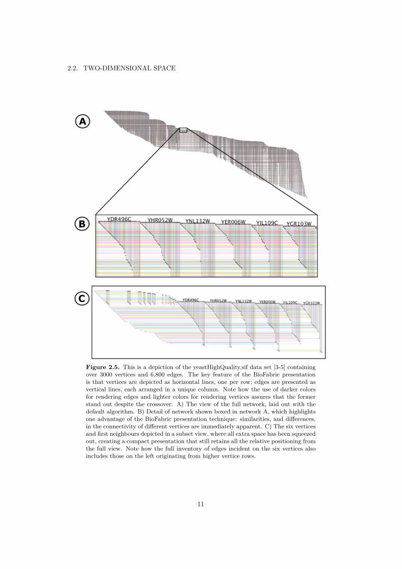
Figure 2.5. This is a depiction of the yeastHighQuality.sif data set [3-5] containingover 3000 vertices and 6,800 edges. The key feature of the BioFabric presentationis that vertices are depicted as horizontal lines, one per row; edges are presented asvertical lines, each arranged in a unique column. Note how the use of darker colorsfor rendering edges and lighter colors for rendering vertices assures that the formerstand out despite the crossover. A) The view of the full network, laid out with thedefault algorithm. B) Detail of network shown boxed in network A, which highlightsone advantage of the BioFabric presentation technique: similarities, and differences,in the connectivity of different vertices are immediately apparent. C) The six verticesand first neighbours depicted in a subset view, where all extra space has been squeezedout, creating a compact presentation that still retains all the relative positioning fromthe full view. Note how the full inventory of edges incident on the six vertices alsoincludes those on the left originating from higher vertice rows.

11


BioFabric has one release which is an open-source Java application with somedocumentation [3]. Though BioFabric is built on a relatively easy and intuitivealgorithm, one could take the option of implementing an own version, having owncustomized features that suits one’s purpose.

Figure 2.6. Layout that tries to place vertices with similar connectivity next to eachother in the linear ordering of vertices.

2.2.2 HivePlots

HivePlots is a visualisation algorithm that uses a number of radially oriented lin-ear axes that have a coordinate system based on vertices properties. A network’svertices are layed out on these axes. Connecting vertices are shown with edges be-tween them, visualized as curves between vertices. Figure 2.7 shows an example ofa HivePlot.

Initially before the layout is made, a number of structural parameters are calcu-lated such as degree, flow, pagerank, clustering coefficient etc. Which parametersto use is up to the user to decide, they need to be appropriate for the networkbeing visualized. For example one could use the clustering coefficient to distinguishbetween hubs and clusters. Next these parameters are used to set up rules that areused to assign vertices to an axis and decide its coordinate. These rules are oftenboolean rules. Example of rules could be:

• Is the vertice a sink?

• Is the vertice a source?

• Clustering coefficient < 0.5?

If a HivePlot can be created with three axes this is preferred [27], laying theaxes with a uniform radial distribution. Because with three axes you get a layoutwere no pair of edges cross each other and no edge connected to two axes will cross

12


Figure 2.7. Example of a HivePlot containing 2500 vertices and 5900 edges.

another axis. Though this is not restrained to only three axes, it becomes hard toassign vertices to axes so these features become obtained for a different number ofaxis.

For HivePlots there are some choices of use, one used is a Java based library[2]. There are also libraries for R [45], HiveR [1], that support HivePlots in thetwo-dimensional and three-dimensional space. The framework D3.JS [14] is anotheroption that is a JavaScript to create hive plots. And pyveplot [43] is a library forHivePlots in Python [44].

2.2.3 TreeMap

TreeMap is a technique to present graphs in sequences of nested boxes [24]. TreeMaprequires the data to be hierarchy structured as a tree. Figure 2.8 shows an example.The size of individual boxes becomes significant in a TreeMap layout, where theuser specifies how they should grow. Take for example if Figure 2.8 shows data thatrepresents a file system. The size of a box could then be proportional to the size ofthe file it represents. The colors of the boxes represent the hierarchy, same color ofboxes belong to the same file.

For TreeMaps there are some choices to make. For .Net, which is this thesi’sworking environment, there is the WPF TreeMaps & SquarifiedTreeMaps controllibrary [11], though it has poor documentation. Another alternative is the .NETTreemap Control library [15]. Here again the problem lies in little documentation

13


and it is hard to get information about the library when it was part of an oldMicrosoft research project called Netscan.

Figure 2.8. Example of a Tree-map

14

2.3. THREE-DIMENSIONAL SPACE

2.3 Three-dimensional spaceIn the hope of aquiring more space for the layout of a network one can take theapproach to go from a 2D to a 3D environment. In other words one can strive toget away from the Euclidean space to another space that provides more dimensions.An important aspect that follows from going to a 3D view is that the system shouldbe nagivatable. This because in a 3D view, vertice and edge occlusion is bound tohappen. Being able to alter a view by navigating becomes an important tool thathelps to find a view where no occlusions occur.

Hyperbolic space

The hyperbolic space has the property that it has more room compared to thefamiliar Euclidean space [37]. [60] states that the fifth postulate in the Euclideanplane geometry can be formulated as:

“Through a given point, not on a given line, one and only one line canbe drawn which does not intersect the given line.”

As in the hyperbolic plane geometry they introduce the Characteristic Postulate:

“Through a given point, not on a given line, more than one line can bedrawn not intersecting the given line.”

Moreover two lines that are parallel in the Euclidean space are always the samedistance apart. As in the hyperbolic space parallel lines are not equidistant. Forinstance two parallel lines in the hyperbolic space that do not intersect can beseperated by increasing distance the further away one moves from the origin. Figure2.9 shows this compared to the Euclidean geometry.

Figure 2.9. Parallel lines in Euclidean space are always the same distance apart. Inhyperbolic space the distance between two lines that never meet does indeed change.Here we show two geodesics which never meet but are not equidistant: the furtherthey extend away from the origin, the more room there is between them.

15


Normally to make use of the hyperbolic space, to use the extra space, one goesabout to perform a layout algorithm in the hyperbolic plane or space and thendisplay the results in the Euclidean plane or space. Some models to do this havebeen created. Best known are the Klein and the Poincaré models [24].

2.3.1 GerbilSphere

There have been studies on 2D vs 3D user interfaces that have shown that in manycases 2D exceeds 3D. Though the more space in 3D is still compelling. GerbilSphereis an inner sphere 2D system that tries to use the benefits from both a 2D approachas well as a 3D approach.

GerbilSphere works in a way that it places the observer inside a sphere whileprojecting the network on to the surface of the sphere. As part of the layout, Ger-bilSphere uses an extended version of the Fruchterman and Reingold force-directedalgorithm to apply to the three dimensional space. However this is not enough towork on the surface of a sphere. To apply the forces to the surface of a sphere, Ger-bilSphere uses an algorithm described by Kobeourov and Wampler [25]. For moretechnical information about the data structure and how their layout algorithm workssee [48].

Zooming in GerbilSphere is viewed as having a world camera attached to oneend of a tether and having the other end attached to the center of the sphere. Whenzooming in and out it can be seen as moving the world camera along this tether.Figure 2.10 shows when zoomed out respectively zoomed in.

Figure 2.10. Spherical volume grid based

GerbilSphere implements a 2 1/2D interface, advocated by Ware [58]. Whena user is positioned inside the sphere and zooms in, the part of the network whenzoomed in will be visualized on a flat 2D surface, as seen in Figure 2.11. Whenzooming out one can still have the point of interest in view, trying to gain moreglobal context of the network. Lastly one can zoom out enough to place the viewoutside the sphere, seeing the network on a 3D sphere.

GerbilSphere is an open-source project. No API is available, though good doc-umentation is presented within the code.

16

2.3. THREE-DIMENSIONAL SPACE

Figure 2.11. Spherical volume grid based

2.3.2 H3: laying out large directed graphs in 3d hyperbolic spaceT. Munzner [37] visualizes graphs in the three-dimensional hyperbolic space byplacing the network, represented as a spanning trees, inside a sphere. It is exploitingthe property that the amount of space covered by a sphere in the three-dimensionalhyperbolic space increases exponentially with respect to the radius of the sphere,rather than polynomially. They compare using the traditional cone trees with theiruse of a layout on spherical caps, see Figure 2.12. Figure 2.13 shows an example ofa network being displayed from [37].

Figure 2.12. Comparison of the traditional cone tree layout along the circumferenceof a circle with the H3 layout on the surface of the spherical cap. Both pictures show54 child vertices in hyperbolic space, represented by pyramids of the same size. Left:The traditional perimeter layout requires a large cone radius and is quite sparse.Right: A quite small cone radius suffices for the H3 spherical cap, so the layout isreasonably dense.

17


Figure 2.13. Link structure of a Web site laid out in Three-dimensional hyperbolicspace by [37]. The vertices represent documents, which are coloured according toMIME type: HTML is cyan, images are purple, and so on.

2.4 Looking forward

When this thesis has been done within a time constraint all the relative methods ofvisualisation could not be implemented and evaluated due to the great number ofexisting methods. Still measures needed to be taken so that no major or relevantvisualisation method gets overlooked. With the information presented in this chap-ter as a basis, the visualisation techniques of the highest relevance will be chosenfor evaluation.

Space

One important choice of consideration is in which space should the networks bedisplayed? In this chapter the reader was introduced to a number of differentspaces where the two most common spaces, the two- and three-dimensional space,are of great importance and need to be included for this thesis purpose.

Different visualisation techniques will behave differently and result in havingdifferent aspects and characteristics depending on which space one uses. These can

18

2.4. LOOKING FORWARD

then be compared for evaluation purposes, such as how layout of vertices and edgesdiffers and what impact the space has on zooming and panning. Also how labelclutter behave in different spaces may be of interest.

Layout method

When it comes to choosing which layout methods to evaluate, the same aspectsmentioned in the previous section need to be considered here as well. Which layoutmethod one chooses to use can have an immense impact on these aspects. Theirresults may also differ depending on which space one use and it needs to be takeninto consideration.

Chosen views

From the research and study in this chapter a selection narrowed down to threedifferent views were made to be used for a implementation of an application. In thisselection both the two-dimensional and the three-dimensional space were covered.We will show the resulting application and for each view give an account of whythose views where selected and how they were implemented in section 4.2.

Technical aspects

In addition to the effects on visualisation from the above described aspects thereare other more practical aspects to be considered. Aspects revolving around oneenforcing some pretension on the performance of the chosen methods implemented.This to ensure smooth usage so that a slow visualisation application will not impactthe result in a negative way when evaluating a visualisation technique. More aboutthis in section in the next chapter and appendix A.

19

Chapter 3

Method

When one is to display data using graphs one is confronted with the task of choosingbetween a large range of different visualisation techniques. This chapter is intendedto show the process used to decide which methods and areas are to be investigatedfor this thesis. In section 3.1 the way found to implement these choices for furtherevaluation is shown. In section 3.2 the way taken for evaluation is described.

3.1 Implementation

It is difficult to compare and evaluate different visualisation techniques only onthe information found in scientific thesis and books concerning them. One causeto this arises when one looks at the data used, different theses use different data.In some cases data might seem bias as having been chosen to fit better with thevisualisation method concerned for the purpose of that particular thesis, making ithard to compare performance between techniques. Different visualisation methodsperform differently on different data, making it only helpful if one wants to establishsome form of knowledge around that a specific technique can be good on a specifickind of data. For this thesis it was necessary to have a more generalized unbiasedapproach.

To work around this an implementation was to be made that incorporates aselection of the studied techniques. Following the methodologies of selection forspaces and layout methods discussed earlier. This in order to make it possible todisplay the same networks (same data), using these different techniques and thenbe able to compare and evaluate performance on these techniques.

3.1.1 Programming environment

The implementation was to be developed in the programming language C# (C-sharp) [33] within Visual Studio [34]. The main application was to be made as anWPF (Windows Presentation Foundation) [36]. Other programming languages thathave been used and incorporated in to the main WPF application is C++ [13] and

21

CHAPTER 3. METHOD

Java [53]. For database retrieval LINQ (Language-Integrated Query) [32] has beenused.

3.2 EvaluationIn order to draw some relevant results from this thesis it is necessary to evaluatethe different visualisation techniques chosen to be investigated. Section 3.2.1 takesup the necessity to adding tests concerning the prerequisites for implementing thelayout views, which programming libraries to use. Section 3.2.2 will explain differentaspects that need to be considered when evaluating the different layout methods.

3.2.1 Programming librariesAn evaluation of different programming libraries was made to find a good startingpoint for the implementation of an application. First a study that investigateswhat different libraries exists that supports visualisation for different networks wasmade. In this research a comparison of which different functionalities these librariessupport was retrieved in form of data structures and algorithms, layout algorithmsand so on.

From this initial study a selection of possible libraries to use for implementationwas needed to be made. From here one could then evaluate the different selectionsto be able to make a final choice of which libraries to use.

The library evaluation will test for the libraries capacity in speed, how muchtime does it take to set up and draw networks of different sizes? And then as the laststep was to evaluate the performance of the libraries after the networks had beendrawn. This by taking measurements of smoothness while traversing a network.Smoothness was represented by the applications FPS (Frames Per Second) whilenavigating the network at different stages. The evaluation of programming librariescan be found in appendix A.

3.2.2 Layout viewsBased on the study done in chapter 2 the different views will be evaluated on thefollowing characteristics that are of great importance for a general visualisationsystem:

• Navigation

• Situational awareness

• Ease of recognizing important parts as sub-networks, vertices and connections

• Labeling

The evaluation will be executed by using the implemented application to try andcomplete tasks similar to the following:

22

3.2. EVALUATION

• Identify cluster/vertice X. Navigate to cluster/vertice Y. Can one navigateback to X?

• Identify the biggest cluster

• Identify vertice X

• Identify the vertice with highest degree

The tasks will be viewed as completed correctly, incorrectly or uncompleted. Inaddition to this, time will be taken into consideration as a measurement of perfor-mance. The results and drawn conclusions from these evaluations can be found inchapter 5.

3.2.3 DataTo be able to perform these evaluations some data needs to be at hand, data thatfits this thesis purpose. This thesis has been performed at a company that providedthe necessary data to be visualized.

Data for evaluation of programming libraries

For the performance evaluation of programming libraries data were needed to begenerated. To generate this data the program Gephi [19] was used. This programwas to be used to generate a number of different graphs of different sizes which werethen saved as a plain text file. The following graphs were generated:

• Graph with 50 vertices with 592 edges. Referred as G50.




On the account that different libraries use different ways of representing datathis text file cannot be presumed to work as input for all libraries. On that factparsers were needed to be developed to attend that the input was on the rightformat for the corresponding library.

Data for layout views

For the layout views, data in the form of electronical units found inside trucks calledECUs (Electronic Control Units) are used. Also variables used within these systemscalled AEs (allocation elements) are used to be visualized.

Their data have a complex form with a great number of relations and commu-nications, thus making it suitable as data for this thesis purpose.

23

Chapter 4

Results

This chapter narrates the results from the literature studies and based on the appli-cation that was implemented. The results from an evaluation of existing program-ming libraires are given in section 4.1. For a more ingoing review of these librariesand how they were evaluated see appendix A. Section 4.2 shows the resulting ap-plication from the implementation and its views.

4.1 Library performanceTo be able to make a solid application that can be used for this thesis evaluations,not only the need of choosing what layout methods to be used needs to be considered.Which prerequisites one chooses to use while implementing said application needsto be considered. Thereby a consideration of which libraries one can use whenimplementing the different visualisation methods is needed.

4.1.1 Attribute matrixThe following matrix, figure 4.1, lists important functionality one looks for whenconsidering a programming library for implementing visualisation methods. Thematrix gives an overview of what the different libraries supports from the start.This matrix helps as a basis when selecting libraries for the implementation.

25

CHAPTER 4. RESULTS

Table 4.1. Attribute matrix

4.1.2 Results from library testsSpeed

Each graph has been drawn ten times and the arithmetic mean value of the timehas been calculated and given as result. Time is displayed on the form of min-utes:seconds.

Table 4.2. Speed results

G50 G100 G500 G1000GraphX 0:0.515 0:7.415 22:33.457 Out of memoryVTK 0:0.0155 0:0.0414 0:0.883 0:3.530yFiles 0:0.540 0:1.682 0:49.605 12:11.536

Smoothness - FPS(Frames per second)

There are three FPS measurements for each library in which panning actions werebeing performed. One zoomed out far away, giving an overview of the graph (Z1),one zoomed in half way to the centre of the graph (Z2) and a third in which the useris zoomed far in to the graph, being able to distinguish between vertices (Z3). Whenthe measurement states undetectable the fps value have been too low to measure,stalling out the program. The procedure this was performed in is the same as forthe speed values, an arithmetic mean value is given.

26

4.2. APPLICATION

Table 4.3. GraphX

Z1 Z2 Z3G50 17 fps 23 fps 35 fpsG100 1 fps 3 fps 5 fpsG500 Undetectable Undetectable UndetectableG1000 Out of memory Out of memory Out of memory

Table 4.4. VTK

Z1 Z2 Z3G50 1000 fps 1000 fps 1000 fpsG100 500 fps 500 fps 500 fpsG500 35 fps 11 fps 3 fpsG1000 11 fps 7 fps 2 fps

Table 4.5. yFiles

Z1 Z2 Z3G50 22 fps 20 fps 25 fpsG100 2 fps 3 fps 5 fpsG500 Undetectable Undetectable UndetectableG1000 Undetectable Undetectable 2 fps

From the tables above one can see that The Visualization Toolkit (VTK) [57]often outperforms the other libraries by a large factor, both in speed and fps mea-surements. Therefore this will be the library of use when implementing own views.

4.2 ApplicationThis section shows the resulting application implemented with the correspondingviews chosen from the research done in chapter 2.

4.2.1 Main applicationAt the start up of this application the user will be taken to the main applicationwhere the user will be prompted to make some choices before being able to visualizedata. These choices are concerning which data to be used.

In this application the user is constrained to choose between visualising ECUsor AEs, see section 3.2.3. The user is also prompted to choose which SOP date touse. Next the user needs to load the data from the database by pressing a button,labeled "Load Data". After that is done the user can go on and choose which viewto display. The user is not restrained to one view at the time but can bring upmultiple views at the same time, making it easy to compare views.

27

CHAPTER 4. RESULTS

4.2.2 Force-Directed (FD) based viewForce-directed algorithms are, as shown in chapter 2, an important part when itcomes to viualising networks. There are many visualisation techniques based solelyon force-directed algorithms and other techniques that use different approachesdo often incorporate some kind of force-directed algorithm to their visualisationmethod. As for example by computing a base graph using a force-directed algorithm.Therefore the first view of the implementation is a view that uses a force-directedalgorithm for the vertices layout and edge routing. Figures 4.1 to 4.6 show examplesof the application using this view.

Figure 4.1. An unlabled overview of a network when all AE was chosen.

28

4.2. APPLICATION

Figure 4.2. Same network as in 4.1 after zooming actions were preformed.

Figure 4.3. A labled overview of a network when all ECUs were chosen.

29

CHAPTER 4. RESULTS

Figure 4.4. Same network as in 4.3 after zooming actions were preformed.

Figure 4.5. Showing data with labels enabled.

30

4.2. APPLICATION

Figure 4.6. Showing same data as in picture 4.5 but with lables unenabled.

Layout

The force-directed view results in an even distrubution of all the vertices and isgood at separating subgraphs from each other, as seen in figure 4.3. An evidentproblem that arises is with the edges of a network. The edges quickly converge toa hairball of edges, making it impossible to distinguish between individual edges.This can be seen in figure 4.2.

Labeling

As mentioned in section B.1.1, the VTK library displays labels according to theirweight, the higher the weight the higher priority a given vertice label will have. Thiscombined with the force-directed algorithm by nature is good at evenly spreadingout vertices, label obscuration becomes less of a problem. An example of this isshown in figure 4.4 where a fairly large network is being displayed.

Of course this comes at a price. By allowing a prioritizing of which labels todisplay one is left with a loss of information, in this case a loss of labels. This canhave a large effect on the outcome result when using this application. Dependingon what tasks one wants to solve by using this visualization technique, importantdata may be missed and/or be more difficult to locate. It comes down to what dataone is attempting to extract from the view. If for instance one is out to identifythe vertices with a large number of connections and greater subnets this view mightwork terrific. On the other hand if one is to find a specific data part that may be

31

CHAPTER 4. RESULTS

smaller weighted this view can be difficult and uneasy to use.

Navigation - Situational awareness

The effect on the situational awareness of a user in this view depends highly on whatstage in a task the user is on and what type of task said user is performing. Becausethe view provides a highly zoomable network a user can with a far out zoomed view,combined with the labeling enabled, acquire a good overlook of a given network.

Though when zooming in using this view there comes a point when some dataare lost, there are only so much data that can fit on a screen at the same time. Thiscan diminish the situational awareness for a user and result in a loss of orientation,forcing a user to zoom out to try and see correlations from one part of the networkto another. The user might even have a loss in orientation trying to get back to thesame spot as before a given zooming action was made. One can draw the conclusionthat this view provides a poor solution for problems having a need for global contextand local details at the same time. This results in a user losing orientation or specificinformation at different stages performing tasks.

In this view one has the option to navigate through the x- and y-axis or x-, y-and z-axis. This can be helpful when looking closer on how a subpart of a networkjoints with another. But one needs to be careful when going from two axses tothree, due to the fact that it can result in a loss of orientation.

4.2.3 Two-dimensional view - BioFabricFor a view in the two dimensional space BioFabric was used. BioFabric providesa non conventional approach to visualize data and have worthy attributes to beevaluated for visualization. Such as the layout algorithm for vertices and edges,the labeling of vertices and how one navigate the network. Figures 4.7 to 4.9 showexamples when using the Biofabric view.

32

4.2. APPLICATION

Figure 4.7. An overview of a network using the BioFabric view when all ECUs werechosen.

Figure 4.8. Same network as in 4.7 after zooming and selection actions were pre-formed.

33

CHAPTER 4. RESULTS

Figure 4.9. Another example of a selection within the network.

Layout

Because of the static layout function BioFabric usess it results in a consistency whilevisualizing graphs, a specific graph will be drawn the same way from one time toanother. One benefit with BioFabrics layout is to get away from the problem ofedge crossings, as seen in the top part of figure 4.8.

BioFabric produces compact graphs, which makes it more difficult to identifyindividual elements without deeper zooms. Comparing the main view with thenetwork overview in figure 4.8, a situation occurs where a greater zoom is neededto see individual elements in a small selection.

Labeling

BioFabric also uses a weighted label solution. Here the vertices with highest degree,as in BioFabric becomes the horizontal lines at the top of the view, will be of thegreatest size. In figure 4.7 one can see this clearly. The reason behind weightinglabels becomes fairly obvious when one starts to think about how it would turnout if BioFabric would try to show all their labels of all vertices at the same size.There would be so many labels occluding each other that one would not be ableto distinguish which label belongs to which vertice. Furthermore most part of thegraph would have labels occluding each other, making it difficult to see what labelsays what.

34

4.2. APPLICATION


BioFabric’s approach is to have more active views in their application at the sametime, they have three different views. One main view of the network, a second viewthat gives an overview of the network and shows selections made and a third viewcalled the network magnifier. The network magnifier displays a sub selection of thenetwork made by the user (a selection) where the user can see all the labels andconnections of vertices in their selection. Figure 4.9 shows all three views where anselection has been made.

Having these different views, especially the relation between the overview andnetwork magnifier, tries to help toward good situational awareness. The user canget a more detailed view of a subpart of a network using the network magnifierwhile trying to maintain a global context by simultaneously looking at the networkoverview and main view.

Having this setup one can argue that their approach goes toward data on de-mand. Requiring the user to have good knowledge about the network being dis-played but also to have a good idea of the where and how the information searchedis localized. Putting the pressure on the user to have a good situational awarenessorientation beforehand, which is not always the case.

4.2.4 Three-dimensional view - GerbilSphereThe direction many new visualisation techniques are taking is attempting to takeadvantage of the extra space in the three-dimensional space. And thus it is ofsignificance for this thesis to incorporate a tree-dimensional visualisation technique.Many of these tree-dimensional techniques use a sphere shape to visualize networksin/on. And it is common that they use some sort of force-directed algorithm tolayout the vertices and edges in this spherical space.

For this application a tree-dimensional view with a layout method that uses thespherical space was used. The view is based on GerbilSphere [48] where the verticesof a network are laid out on the surface of a sphere and one navigates from a pointof view inside the sphere (though one can zoom out to see the sphere from theoutside). For more details about GerbilSphere see chapter 2 section 2.3.1. Figure4.10 and 4.11 show the view in use zoomed outside the sphere while figure 4.12shows the view from inside the sphere.

35

CHAPTER 4. RESULTS

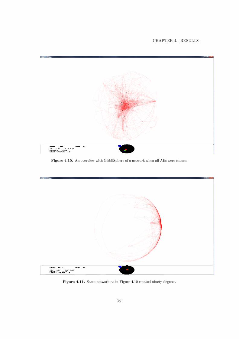
Figure 4.10. An overview with GirbilSphere of a network when all AEs were chosen.

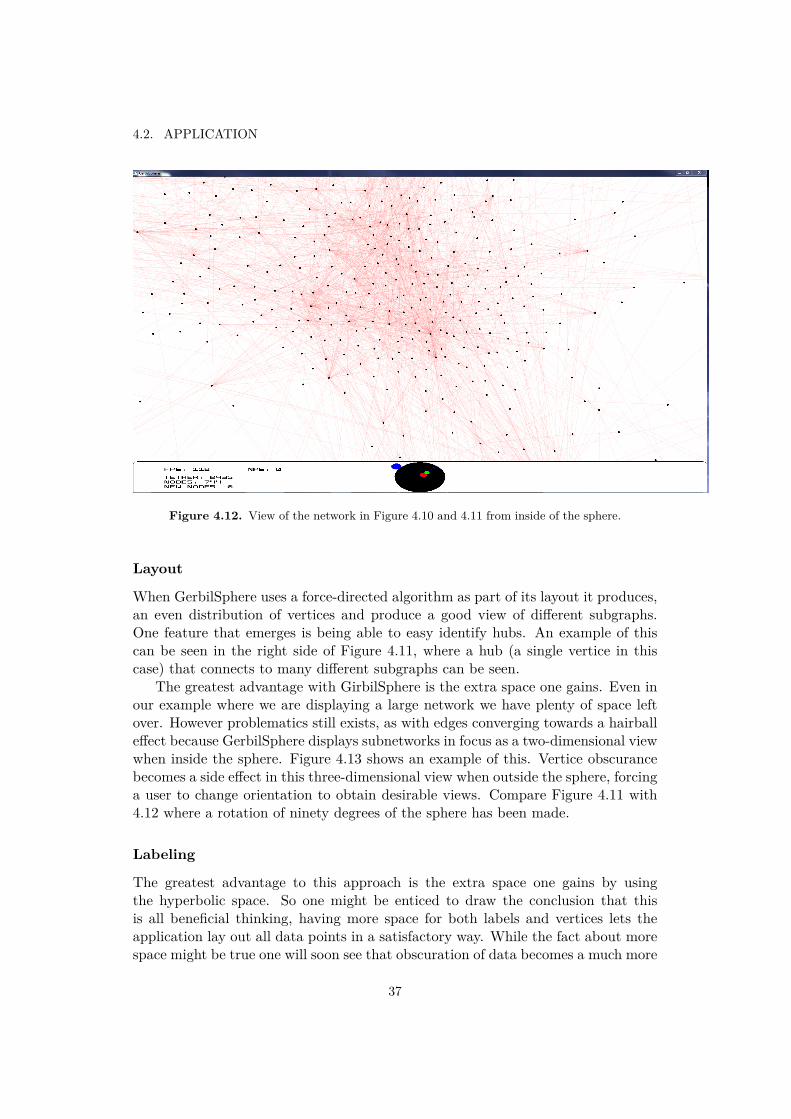
Figure 4.11. Same network as in Figure 4.10 rotated ninety degrees.

36

4.2. APPLICATION

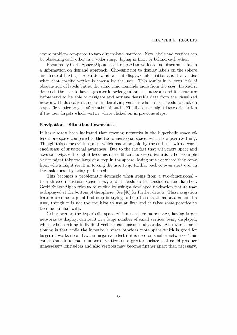
Figure 4.12. View of the network in Figure 4.10 and 4.11 from inside of the sphere.

Layout

When GerbilSphere uses a force-directed algorithm as part of its layout it produces,an even distribution of vertices and produce a good view of different subgraphs.One feature that emerges is being able to easy identify hubs. An example of thiscan be seen in the right side of Figure 4.11, where a hub (a single vertice in thiscase) that connects to many different subgraphs can be seen.

The greatest advantage with GirbilSphere is the extra space one gains. Even inour example where we are displaying a large network we have plenty of space leftover. However problematics still exists, as with edges converging towards a hairballeffect because GerbilSphere displays subnetworks in focus as a two-dimensional viewwhen inside the sphere. Figure 4.13 shows an example of this. Vertice obscurancebecomes a side effect in this three-dimensional view when outside the sphere, forcinga user to change orientation to obtain desirable views. Compare Figure 4.11 with4.12 where a rotation of ninety degrees of the sphere has been made.

Labeling

The greatest advantage to this approach is the extra space one gains by usingthe hyperbolic space. So one might be enticed to draw the conclusion that thisis all beneficial thinking, having more space for both labels and vertices lets theapplication lay out all data points in a satisfactory way. While the fact about morespace might be true one will soon see that obscuration of data becomes a much more

37

CHAPTER 4. RESULTS

severe problem compared to two-dimensional soutions. Now labels and vertices canbe obscuring each other in a wider range, laying in front or behind each other.

Presumably GerbilSphereAlpha has attempted to work around obscurance takena information on demand approach. Choosing not to display labels on the sphereand instead having a separate window that displays information about a verticewhen that specific vertice is chosen by the user. This results in a lower risk ofobscuration of labels but at the same time demands more from the user. Instead itdemands the user to have a greater knowledge about the network and its structurebeforehand to be able to navigate and retrieve desirable data from the visualizednetwork. It also causes a delay in identifying vertices when a user needs to click ona specific vertice to get information about it. Finally a user might loose orientationif the user forgets which vertice where clicked on in previous steps.


It has already been indicated that drawing networks in the hyperbolic space of-fers more space compared to the two-dimensional space, which is a positive thing.Though this comes with a price, which has to be paid by the end user with a wors-ened sense of situational awareness. Due to the the fact that with more space andaxes to navigate through it becomes more difficult to keep orientation. For examplea user might take too large of a step in the sphere, losing track of where they camefrom which might result in forcing the user to go further back or even start over inthe task currently being performed.

This becomes a problematic downside when going from a two-dimensional -to a three-dimensional space view, and it needs to be considered and handled.GerbilSphereAlpha tries to solve this by using a developed navigation feature thatis displayed at the bottom of the sphere. See [48] for further details. This navigationfeature becomes a good first step in trying to help the situational awareness of auser, though it is not too intuitive to use at first and it takes some practice tobecome familiar with.

Going over to the hyperbolic space with a need for more space, having largernetworks to display, can reult in a large number of small vertices being displayed,which when seeking individual vertices can become infeasable. Also worth men-tioning is that while the hyperbolic space provides more space which is good forlarger networks it can have an negative effect if it is used on smaller networks. Thiscould result in a small number of vertices on a greater surface that could produceunnessesary long edges and also vertices may become further apart then necessary.

38

Chapter 5

Discussion and Conclusions

In this chapter plausible conclusions from the studies and results in previous chap-ter will be discussed to answer this thesis question. Which type of visualisationtechnique is best suited to visualize big and complex networks?

5.1 Which type of visualisation technique is then bestsuited to visualize big and complex networks?

One thing that becomes fairly clear when reading the research from this thesis isthat answering this question is not an easy task. Due to the fact that this thesisdoes not go through all existing visualisation techniques, the evidence from thisthesis points toward the conclusion that there is no correct solution answering thisquestion. It points more towards that there is no best choice of technique to displaya complex network that is independent from the kind of and form of data beingused.

It boils down to that when one wants to visualize a complex network one mustconsider all the features and demands that the given network needs. Do we needmore space for the data? A clean and clear structural way of traversing the net-work? How does the need for labeling our vertices look? Do we need to find out howsubnetworks looks like or get more information about specific vertices and connec-tions? And so on. There exists an indefinite number of different complex networksand one cannot find a generalisation saying that one visualisation technique satisfiesall the needs of all networks and displays them in an optimal way.

Instead one needs to tailor a specified solution for a specific network and the ac-companied requirements of visualisation with it. One needs to become very familiarwith the data that is going to be displayed along with getting an excellent knowl-edge of the visualisation needs for the specific application. Then use this knowledgeto develop features that comply with these needs. Features such as complex filtersthat trim the network to specific data, search functions, highlights etc. It all boilsdown too the needs of the specific application.

39

CHAPTER 5. DISCUSSION AND CONCLUSIONS

For further research one could be interested in seeing how these different vi-sualisation approaches would cooperate. To see how the situational awareness isaffected when navigating through one view and seeing at the same time that changein the different views. How it would affect if one takes a sub-selection of a networkin one view and sees the same sub-selection marked in the other views simultane-ously. Filters may become important features when it is often hard to draw anygood information from looking at a entire network at once. Often one is lookingfor a subgraph and needs a more detailed view of said graph. Such filters could bedeveloped that take keywords describing features one are looking for. Or maybe itis better for the user to first see the whole network and manually make selections?Being able to create filters for not only vertices but also edges could be evaluated.Would letting the user decide which types of connections to display help gettingaway from the hairball of edges problem? These kind of questions needs to be askedand answered when developing a visualization technique or application.

5.2 Environmental aspectsIt is hard to draw any definite conclusions on the impact this thesis work has onenvironmental aspects, at the time this thesis was completed no mentionable effectshad occurred. Though it is known that visualisation of complex networks canhelp too facilitate work with analysis and verification of the systems the networksrepresent. In this case this could lead to safer and more cost-effective vehicles. Thisbecomes particular important in the case of autonomous heavy vehicles. Thereforeif work is continued from this thesis one could see these impacts in the future.

40

Appendix A

Library evaluation

A.0.1 Libraries of interestFor the considered libraries of use for the implementation four different categories isused to classify them. Open-source libraries, closed-source libraries, 3D-approachesand non-conventional graph visualisation approaches.

Open-source libraries

QuickGraph

QuickGraph [9] is a library containing generic graph data structures and algorithmsfor a range of graph problems, developed for .Net [55] use. Such as classical prob-lems like maximum flow, topological sort, shortest path, depth search, etc.

Supports: [8]

1. Graph data structures

1.1. Directed graph1.2. Undirected graph1.3. Dense graph1.4. Sparse graph

2. Graph computational Algorithms

2.1. Topological sort2.2. Strongly connected components2.3. Minimum spanning tree

Notes:

41

APPENDIX A. LIBRARY EVALUATION

QuickGraph does not support an option to use an own solution for visualisationof graphs but points to the layout library Graphviz [22] that QuickGraph claimswork well with their data structures [10]. This applies to layout algorithms as well.

Graphviz

Graphviz [22] - graph visualization software. Graphviz provides different layoutalgorithms and take descriptions of graphs in a text language as input. Normalusage with Graphviz is by using DOT (graph description language) [51].

It can be used with QuickGraph as a C# wrapper. Other wrappers for C# and.Net one could use are graphviznet [6] and graphviz4net [7].

Supports:

1. Layout algorithms [22]

1.1. Dot1.2. Neato1.3. Fdp1.4. Sfdp1.5. Twopi1.6. Circo1.7. Osage

GraphX

GraphX is an advanced open-source .Net library for graph visualization with capa-bilities to rend large graphs with large amount of vertices and edges which dependson the QuickGraph library [42]. It also uses partial code from Graph# [21], WPFEx-tensions [12], NodeXL [38] and Extended WPF Toolkit [61], which are open-sourceprojects.

It is based on WPF for rendering graphs and can be seen as the successor tooGraph#. GraphX is the new Apache Sparks API for graphs and graph-parallelcomputation. It introduces a new API that operates on both tables and graphsand incorporate this API as a library using graph parallel techniques to be as fastas specialized systems (such as GraphLab, Giraph and Pregel). By embedding thisgraph-parallel model in Spark it enables GraphX to integrate easily with RDDS(Resilient Distributed Datasets: A Fault-Tolerant Abstraction for In-Memory Clus-ter Computing) and perform data parallel operation while also enabling the speedof specialize graph systems [62].

42

Supports: [42]

1. Layout algorithms

1.1. BoundedFR (Fruchterman Reingold).1.2. Circular.1.3. CompoundFDP.1.4. EfficientSugiyama.1.5. Sugiyama.1.6. FR.1.7. ISOM.1.8. KK (Kamanda and Kawai).1.9. LinLog.

1.10. Tree.

2. Possibility to implement an own layout algorithm (external layout algorithm).

3. Visual control

3.1. Delete animation of vertices and edges.3.2. Mouse over control animation3.3. Custom animations3.4. Highlighting of vertices and edges.3.5. Zoom control.3.6. Area selection of vertices.3.7. Area zooming and smooth animations.

Notes:

There is no documentation of implemented functions for nested graphs. A nestedgraph is a graph were vertices can contain subgraphs within themselves.

MSAGL

MSAGL [46], Microsoft Automatic Graph Layout, is a .Net tool for graph lay-out and viewing. It is built on the Sugiyama scheme [54] that produce hierarchicallayouts. Where the vertices are drawn in horizontal layers and the edges are oftendrawn in a downward fashion between vertices. MSAGL contains its own layoutengine.

Supports: [46]

43


1. Layout algorithms.

1.1. Sugiyama.

2. Editable layout after initial layout.

3. Navigation of graph

3.1. Zoom.3.2. Pan.3.3. Search and focus function.

4. Visual control.

4.1. Highlighting of vertices.4.2. Zoom.

Closed-source libraries

yFiles(yWorks)

yFiles [66] provides data structures and algorithms for graph operations. Includingautomatically layouts for graphs and visualization controls for those graphs. yFilesare supported for different platforms, including .Net where one can either use alibrary for Windows Forms [35], WPF [36] or Silverlight [49].

Supports: [65] [64] [63]

1. Layout algorithms

1.1. Circular layout.1.2. Hierarchical layout.1.3. Organic layout.1.4. Orthogonal layout.1.5. Tree layout.1.6. Incremental layout.

2. Edge routing algorithms.

2.1. Organic routing.2.2. Orthogonal routing.

3. Visual control.

44

3.1. Highlighting controls.3.2. Zoom.3.3. Smooth change animations.

Notes:

yFiles also supports incremental layout, meaning that when a graph needs to beupdated (addition/removal of vertices or edges) the whole graph is not re-computedbut tries to maintain as much as possible of the same layout as before. Also yFilestries to supports nested graphs, but has some restrains on the data to be able touse it. Their function is called collapsible tree, which requires the data to be ableto be structured as a tree.

An comparison of given libraries.

Attribute matrix:

The following matrix, figure A.1, lists important functionality one looks for whenconsidering a programming library for implementing visualisation methods. Thematrix gives an overview of what the different libraries supports from the start.This matrix helps as a basis when selecting libraries for the implementation.

Figure A.1. Attribute matrix

3D approaches

Libraries

For developing advanced 3D graphics the two most common approaches is to useeither OpenGL [41] or Direct3D [31]. To use OpenGL in windows one has a fewoptions, one can for example use OpenTK that wraps OpenGL, OpenCL [39] andOpenAL [40].

45


Direct3D is part of the DirectX API that uses hardware acceleration (if availableon the graphics card).

Differences between OpenGL and Direct3D

OpenGL is being developed largely by a consortium of different parties and followsa largely open standard. While Direct3D are being developed and maintained byMicrosoft and is completely proprietary in its implementation. Resulting in a bigplatform difference, where OpenGL is supported on a wide range of platforms andlanguages, while Direct3D is bound to Microsoft Windows systems.

At last there are different methods used to introduce new hardware and features.OpenGL do this by allowing hardware manufactures to be able to implement specialfunctions, called extensions that give immediate access to features of new hardware.As for Direct3D, Microsoft needs to process theses features and then release access tothese in forms of new functions. Here OpenGL allows new features to be accessiblequicker then Direct3D, though reduces the overall compatibility of a program usingthe extensions. And the other way around, Direct3D takes longer to give access tothe new features but compatibility across different systems is being maintained.

The aspect of hardware managing differs in these two libraries. OpenGL hidesthe hardware and works so that the implementation handles hardware resources,users of OpenGL use functions for drawing which relies on drivers to directly accessthe hardware. Direct3D on the other hand lets the application handle the hardwareresources. With OpenGL it becomes easier to write applications but hard to seethe status of hardware resources and thus must hope that the implementation usesthe resources in a way that suits the related application. While with Direct3D thewriting of the application may be more complex but have the possibility to usehardware resources in the most efficient way for the application [59].

Both these differs a bit form previous discussed libraries in the sense that thereare no (known) support for graph visualization. So for instance no layout algorithmsfor graphs like force directed or data structures to represent a graph. This impliesthat all has to be implemented from scratch, taking more time but open up for lessrestrictions on what one can do.

VTK

VTK (Visualization Toolkit) [57] is an open-source software system for 3D computergraphics, image processing and visualization. At its core VTK is implemented as aC++ toolkit and it supports parallel processing which help in performance. VTKis a popular library when it comes to visualize scientific data, which is often big andcomplex.

There are a number of wrapper languages making it possible in addition to C++use VTK through for instance Python, Java and .NET.

46

Non conventional graph visualization approaches

When it comes to the visualisation techniques like BioFabric, Hive Plots and Treemap(described in chapter 2) there are few libraries that support this compared to theamount of libraries there are to visualize the classical vertice/edge graphs. Howthese approaches can be used are shown below.

BioFabric:

BioFabric has one release which is an open-source Java application with some doc-umentation that can be found at [3]. Though BioFabric is built on a relatively easyand intuitive algorithm, one could take the option of implementing an own version.Having their own customized features that suits one’s purpose.

Hive Plots:

For hive plots there are some choices, one used is a Java based library [2]. There arealso libraries for R [45], HiveR [1], that supports hive plots in the two dimensionaland three dimensional space. The framework D3.JS [14] is an other option that isa JavaScript to create hive plots. And pyveplot [43] that is a library for hiveplotsin Python [44].

Tree Map:

As for Treemaps there are some choices as well. For .Net, which is this thesisworking environment, there is the WPF Treemaps & SquarifiedTreeMaps controllibrary [11], though it has poor documentation. Another alternative is the .NETTreemap Control library [15]. Again the problem lies in little documentation and itis hard to get information about the library when this was part of an old Microsoftresearch project called Netscan.

GerbilSphere:

GerbilSphere visualize graphs by projecting vertices and edges to the surface ofa sphere, defined as an inner sphere 2D system. It differs from other graph vi-sualisation techniques that also uses spheres in the way that in GerbilSphere theobservers point of view is from inside the sphere.

GerbilSphere is an open source project. No API is available, though good doc-umentation is presented within the code.

Supports: [48]

1. Specialised layout algorithm that is based on force-directed algorithms.

47


1.1. Static layout when adding/removing vertices.

2. Labeling.

3. Menus when choosing specific vertices.

4. Visual control.

4.1. Zoom.4.2. Paning.4.3. Fisheye view.4.4. Variablezoom.

Notes:

While GerbilSphere does not support nested graphs this becomes of less interestwhen the whole graph is being visualized.

A.0.2 Library selection for evaluation

From the matrix in figure A.1 one conclude that GraphX and yFiles are two possiblecandidates for usable libraries. They both support more functionality than Quick-Graph, MSGAL and GraphViz. Therefore they will be included in the evaluation.

Needed is also an option for implementing three dimensional views. For thispurpose the VTK library is included when it has support for graph visualization.

A.0.3 Test set up

The libraries have been tested on two different aspects, rendering speed and smooth-ness. Rendering speed is measured as the time it takes a specific library to draw upa given graph. As for smoothness the frames per second (fps) rate has been mea-sured during navigation through corresponding graphs. Navigation actions such aspanning and zooming.

Data

The data used for these tests has been produced with the use of Gephi [19]. Fourdifferent graphs were created for testing:

• 50 vertices with 592 edges. Referred as G50.




48

Hardware

The evaluations where runned on the same computer for each graph and librarywith the following hardware:

Processor: Intel(R) Core(TM) i5-3470 CPU @ 3.20GHzVideo Card: Intel(R) HD Graphics. 64 MB Dedicated Memory, 1.7 GB Total MemoryMemory: 6.1 GBOperating System: Microsoft Windows 7 Enterprise Edition Service Pack 1 (build 7601), 64-bit

A.0.4 Results from library tests

Two kinds of users need to be considered when talking about the results fromthe library evaluations. The users that will indirect use the libraries by using anapplication built on these, we will call these users for end users. Second is the kindof user that will use these libraries to build an application for visualisation, we callthese users for developer users.

The needs one have on the libraries differs depending on what kind of user oneare. For an end user the speed and smoothness are the two things that shows most.Developer users must also take into consideration what the different libraries sup-ports and not.

Speed

Each graph have been drawn ten times and the arithmetic mean value of the timehas been calculated and given as result. Time is displayed on the form of min-utes:seconds.

Table A.1. Speed results

G50 G100 G500 G1000GraphX 00:00.51461281 00:07.41482771 22:33.4573175 Out of memoryVTK 00:00.01546258 00:00.04138581 00:00.88301525 00:03.53977976yFiles 00:00.54974544 00:01.68249026 00:49.60542746 12:11.535764772

Here one can see that the VTK library is far superior to the other libraries, espe-cially on the larger sized graphs. On the smallest graphs the difference are not assignificant. For the end users the difference on drawing speed on graphs of size with50 vertices would not be to notable. Though the developer users might want to takethis into consideration. On larger than 50 vertices graphs the difference betweenthese libraries shows fairly clear. GraphX drawing speed decreases rapidly and arenot able to draw graphs with a size of 1000 vertices with the hardware used. yFilesdo manage to draw this graph, though it took over 12 minutes compared to VTKs

49


3 seconds.

Smoothness - FPS(Frames per second)

There are three fps measurements for each library were panning actions was be-ing performed. One zoomed out far away, giving an overview of the graph (Z1), onezoomed in half way to the centre of the graph (Z2) and a third were the user arezoomed far in to the graph, being able to distinguish between vertices (Z3).

Table A.2. GraphX

Z1 Z2 Z3G50 17 fps 23 fps 35 fpsG100 1 fps 3 fps 5 fpsG500 Undetectable Undetectable UndetectableG1000 Non-executable Non-executable Non-executable

Table A.3. VTK

Z1 Z2 Z3G50 1000 fps 1000 fps 1000 fpsG100 500 fps 500 fps 500 fpsG500 35 fps 11 fps 3 fpsG1000 11 fps 7 fps 2 fps

Table A.4. yFiles

Z1 Z2 Z3G50 22 fps 20 fps 25 fpsG100 2 fps 3 fps 5 fpsG500 Undetectable Undetectable UndetectableG1000 Undetectable Undetectable 2 fps

50

From these tables one can see that GraphX and yFiles perform almost equally,though VTK outperforms both these libraries with quite a larger margin. VTK isalso the only one that could detect a readable FPS value when maneuvering thelargest sized graph. Both GraphX and yFiles displays a better smoothness (higherFPS) at a deeper zoom, which at first can seem a bit strange. The reason for thisis that once you are zoomed far enough in the graph, you come to a point wherethere is less vertices and edges to display on the screen then previous zoom wherethe low FPS value starts to increase after this point.

To take into consideration

One thing that becomes overlooked when talking about these different libraries ishow one wants to draw graphs. For instance if one wants a small or large repre-sentation of vertices. If one is planing on just drawing smaller graphs with largervertices one might be fine using yFiles or GraphX. Though if one wants to drawgraphs of the larger kind one might be better suited with the VTK library. Theseaspects will of course affect the speed and smoothness when using these libraries.In this study the basic common configuration for each library has been used.

For the end user the speed and smoothness is what becomes of most importance,because that is what they see when using an application. The developer user mustof course take this into account when developing an application. The developer usermust also take into consideration what features that the different libraries support.

51

Appendix B

Implementation details.

B.1 Views

B.1.1 Force-directed(FD) based view

This view was implemented when using the VTK library for C# on the basis fromthe evaluation done in section 4.1.

In this view the user of the application can choose between showing labels ornot. The labeling of the vertices in this view are weighted with a weight based ontheir degree. This in such a way that the higher the degree of a vertice, the higherweight that vertices label will be given. Based on the vertices weights, a priorityof which labels to be displayed at a certain point in the network are made. Givingvertices with higher degree a higher priority. This also results in that depending onwhich zoom level in a network one are, different labels will be prioritised.

When it comes to the space this view is using, it is actually up to the user tochoose. By holding down shift when navigating a network in this view the z-axlebecomes fixed, making it appear as a two dimensional view. Otherwise it works inthe three dimensional space, where one can navigate through the x-, y- and z-axles.This is unique to this view, the next two views works in the two- or three-dimensionalspace.

B.1.2 Two-dimensional view - BioFabric

BioFabric is an open-source Java application which makes it applicable to use forthis thesis. Though some changes was needed to be done for it to work with theimplementation. Changes concerning the code that conducts to where and how theinput of data for the application were made, changes so that BioFabric becomescompatible with the application. Also additions concerning that the input dataconverts to the correct form for BioFabric where needed. More about this in B.2.3.

53

APPENDIX B. IMPLEMENTATION DETAILS.

B.1.3 Three-dimensional view - GerbilSphereGerbilSphere is an open source application developed in C++. Again the datahandled needs to be modified to match the form of data input GerbilSphere usesand more about this in B.2.3.

GerbilSphere handles labels a bit differently than previous views. Instead oftrying to place visible labels in the spherical space they have taken an informationon demand approach, making it up to the user to prompt for specific informationat need. This by having a secondary window up that keeps track of actions made inthe sphere. As when clicking on a specific vertex results in getting the information(the label) about that vertex showing in this window.

B.2 Data representationThis section goes over how to represnt the data to be visualized in the differentviews.

B.2.1 GraphElementTo be able to represent data in the earlier stages, before displaying any views, asmall class called GraphElement was created. This represents, as its name suggests,an element of a graph such as a vertex or an edge.

The class holds parameters about the name and ids and functions that makesit possible to distinguish between two different GraphElements.

B.2.2 Data representation within application - DataManagerDataManager is a class developed to do the actual data retrieval from the workingdatabase. To represent a graph internal in the application the DataManager classretrieves the data one wants to visualise and creates GraphElement objects thatare put into an object of the data structure called Dictionary [30]. This in such away that each object (can be seen as a vertice) of a network will be set as a keyin the dictionary and have a tied value in form of a list of GraphElements. Thusone can see the dataset as a given key (vertice) in the dictionary (network) has acorresponding list Y (neighbours). For instance say that GraphElement X is a keyand are associated to a list Y, then an object y in Y can be seen as that there existsand edge between X and y.

Then when it comes to actually visualise data one needs to convert the datato the appropriate form for the corresponding view. More about this in the nextsection.

B.2.3 Data parsersThis section will give account for the resulting data parser written for each of thethree views. Parser for the VTK library for the force-directed view, a parser for

54

B.2. DATA REPRESENTATION

BioFabric and lastly a parser for GerbilSphereALpha.

VTK data parser

The VTK library uses a straightforward simple way of representing a graph. Itworks in a way that first all the vertices are added and get sequential ids startingfrom 1. Then one can add edges between these by calling a function with parameterssaying between which two vertices the edge connects, using the vertices ids. Makingit very compatible with the DataManager class and GraphElement object.

Because VTK represents their data in such a way and one needs to build thedata structure in code behind there was no need to implement a parser for VTK.One could simply retain the necessary information from your network and use itdirectly to functions for building graphs in the VTK library. Though a parser wasimplemented, reading a text file containing information about a network and storingit in a dictionary, such as in the DataManager class. This parser was implementedfor the evaluation stage for the VTK library. Making it possible to take a text file,generated from Gephi, as input and returning a dictionary that could then be usedto generate a graph with VTK to be evaluated.

BioFabric data parser

BioFabric supports tab-delimited .sif files [4] as input, therefore a parser for trans-forming data from our DataManager class to SIF files were created. A SIF file hasthe following form:

From vertice name, tab pp (indicating an edge), and tab followed by to verticename. For example:2 pp 4,meaning there exists an edge between vertice 2 and vertice 4.

Where it states vertex name, the information in that field will be what displays inthe BioFabric view as the labels.

GerbilSphere data parser

GerbilSphere supports two different file formats as input. First is Pajek [20] andthe second is the Extensible Graph Markup Language (XGMML) [5]. Pajek is ona text based format with the file extension .Net. Which first states the number ofvertices N, followed by N lines with the vertices id and labels. Next comes "*Edges"followed by X lines defining the networks edges. Where the vertices from id areshown followed the to vertice id. The edges can also be weighted, in that case athird value with the weight are added.

In GerbilSphereAlpha these vertices can have attributes such as positioning forthe sphere, the file is then called baked. See [48] for further information.

55

APPENDIX B. IMPLEMENTATION DETAILS.

XGMML is based on the Graph Modelling Language, GML, which is a hierarchi-cal ASCII-based file format for describing graphs. Using tags to describing differentgraph components. Though both Pajek and XGMML where usable for this thesisapplication the Pajek format was in the end used.

A parser for both these file formats where created, following the syntax describedabove.

56

References

[1] academic.depauw.edu. Hiver. http://academic.depauw.edu/~hanson/HiveR/HiveR.html. [Online; Accessed 21-December-2014].

[2] bcgsc.ca. jhive - A Java GUI for Hive Plots. https://www.bcgsc.ca/wiki/display/jhive/home. [Online; Accessed 21-December-2014].

[3] biofabric.org. Biofabric documentation. http://www.biofabric.org/#docs.[Online; Accessed 21-December-2014].

[4] biofabric.org. Sif files. http://www.biofabric.org/#sif. [Online; Accessed27-December-2014].

[5] cgi5. Xgmml (extensible graph markup and modeling language). http://cgi5.cs.rpi.edu/research/groups/pb/punin/public_html/XGMML/. [On-line; Accessed 28-December-2014].

[6] code.google.com. graphviznet. https://code.google.com/p/graphviznet/.[Online; Accessed 19-December-2014].

[7] codeplex.com. Graphviz4net. https://graphviz4net.codeplex.com/. [On-line; Accessed 19-December-2014].

[8] codeplex.com. Quickgraph documentation. https://quickgraph.codeplex.com/documentation. [Online; Accessed 19-December-2014].

[9] codeplex.com. Quickgraph, graph data structures and algorithms for .net.https://quickgraph.codeplex.com/. [Online; Accessed 19-December-2014].

[10] codeplex.com. Visualization using graphviz. https://quickgraph.codeplex.com/wikipage?title=Visualization%20Using%20Graphviz&referringTitle=Documentation/. [Online; Accessed 19-December-2014].

[11] codeplex.com. Wpf treemaps squarifiedtreemaps control. https://treemaps.codeplex.com/. [Online; Accessed 21-December-2014].

[12] codeplex.com. Wpfextensions. https://wpfextensions.codeplex.com/. [On-line; Accessed 15-March-2015].

57

REFERENCES

[13] cplusplus.com. cplusplus. http://www.cplusplus.com/. [Online; Accessed16-December-2015].

[14] d3js.org. D3 data-driven documents. http://d3js.org/. [Online; Accessed21-December-2014].

[15] devx.com. The .net treemap control. http://www.devx.com/xml/Article/17357/0/page/2. [Online; Accessed 21-December-2014].

[16] Peter Eades. A heuristic for graph drawing. Congressus Numerantium, 42:149–160, 1984.

[17] M.R. Endsley. Situation awareness global assessment technique (sagat). InAerospace and Electronics Conference, 1988. NAECON 1988., Proceedings ofthe IEEE 1988 National, pages 789–795 vol.3, May 1988.

[18] T. Fruchterman and E. Reingold. Graph drawing by force-directed placement.Softw. - Pract. Exp., 21(11):1129–1164, 1991.

[19] gephi.org. The open graph viz platform. https://gephi.org/. [Online; Ac-cessed 21-December-2014].

[20] gephi.org. Pajek net format. https://gephi.org/users/supported-graph-formats/pajek-net-format/. [Online; Accessed 28-December-2014].

[21] graphsharp.codeplex.com. Graph#. http://graphsharp.codeplex.com/.[Online; Accessed 19-December-2014].

[22] graphviz.org. Graphviz - graph visualization software. http://www.graphviz.org/. [Online; Accessed 19-December-2014].

[23] R. Hadany and D. Harel. A muli-scale algorithm for drawing graphs nicely.Discrete Applied Mathematics, 113(1):3–21, 2001.

[24] Ivan Herman, Guy Melancon, and Marshall M. Scott. Graph visualization andnavigation in information visualization: A survey. Visualization and ComputerGraphics, IEEE Transactions on, 6(1):24–43, 2000.

[25] S.G. Kobourov and K. Wampler. Non-euclidean spring embedders. IEE Trans-actions on Visualization and Computer Graphics, 11, 2005.

[26] Stephen G. Kobourov. Force-directed drawing algorithms. In Handbook ofGraph Drawing and Visualization, pages 383–408, October 2013.

[27] Martin Krzywinski, Inanc Birol, Steven JM Jones, and Marco A Marra. Hiveplotsârational approach to visualizing networks. Briefings in Bioinformatics,13(5):627–644, 2012.

58

[28] William Longabaugh. Combing the hairball with biofabric: a new approachfor visualization of large networks. BMC Bioinformatics, 13(â1):275, 2012.

[29] Joe Marks and Stuart Shieber. The computational complexity of cartographiclabel placement. Technical report, 1991.

[30] MSDN. Dictionary<tkey, tvalue> class. https://msdn.microsoft.com/en-us/library/xfhwa508(v=vs.110).aspx. [Online; Accessed 27-December-2014].

[31] MSDN. Directed3d. https://msdn.microsoft.com/en-us/library/windows/desktop/hh309466(v=vs.85).aspx. [Online; Accessed 20-December-2014].

[32] MSDN. Linq (language-integrated query). https://msdn.microsoft.com/en-us/library/bb397926.aspx. [Online; Accessed 16-December-2014].

[33] MSDN. Visual c#. https://msdn.microsoft.com/en-us/vstudio/hh341490.aspx. [Online; Accessed 15-December-2015].

[34] MSDN. Visual studio. https://msdn.microsoft.com/sv-se/library/dn762121.aspx. [Online; Accessed 16-December-2015].

[35] MSDN. Windows forms. https://msdn.microsoft.com/en-us/library/dd30h2yb(v=vs.110).aspx. [Online; Accessed 20-December-2014].

[36] MSDN. Wpf. https://msdn.microsoft.com/en-us/library/aa970268(v=vs.110).aspx. [Online; Accessed 16-December-2015].

[37] T. Munzner. H3: laying out large directed graphs in 3d hyperbolic space.In Information Visualization, 1997. Proceedings., IEEE Symposium on, pages2–10, Oct 1997.

[38] nodexl.codeplex.com. Nodexl: Network overview, discovery and exploration forexcel. http://nodexl.codeplex.com/. [Online; Accessed 19-December-2014].

[39] NVIDIA. Opencl. https://developer.nvidia.com/opencl. [Online; Ac-cessed 20-December-2014].

[40] openal.org. Openal. https://www.openal.org/. [Online; Accessed 20-December-2014].

[41] opengl.org. Opengl. https://www.opengl.org/. [Online; Accessed 20-December-2014].

[42] panthernet.ru. Graphx fpr .net. http://www.panthernet.ru/en/projects-en/graphx-en. [Online; Accessed 19-December-2014].

[43] pypi.python.org. pyveplot. https://pypi.python.org/pypi/pyveplot/.[Online; Accessed 21-December-2014].

59

REFERENCES

[44] python.org. python. https://www.python.org/. [Online; Accessed 21-December-2014].

[45] r project.org. What is r? https://www.r-project.org/about.html. [Online;Accessed 21-December-2014].

[46] research.microsoft.com. Microsoft automatic graph layout. http://research.microsoft.com/en-us/projects/msagl/. [Online; Accessed 20-December-2014].

[47] Doug Schaffer, Zhengping Zuo, Saul Greenberg, Lyn Bartram, John Dill,Shelli Dubs, and Mark Roseman. Navigating hierarchically clustered networksthrough fisheye and full-zoom methods. ACM Trans. Comput.-Hum. Interact.,3(2):162–188, June 1996.

[48] David S. Shelley and Mehmet Hadi Gunes. Gerbilsphere: Inner sphere net-work visualization. Computer Networks, 56(3):1016 – 1028, 2012. (1) ComplexDynamic Networks (2) {P2P} Network Measurement.

[49] Microsoft Silverlight. Windows forms. https://www.microsoft.com/silverlight/. [Online; Accessed 20-December-2014].

[50] Wikipedia the free encyclopedia. Cosine similarity. http://en.wikipedia.org/wiki/Cosine_similarity. [Online; Accessed 28-November-2014].

[51] Wikipedia the free encyclopedia. Dot (graph description language). https://en.wikipedia.org/wiki/DOT_(graph_description_language). [Online;Accessed 19-December-2014].

[52] Wikipedia the free encyclopedia. Jaccard index. http://en.wikipedia.org/wiki/Jaccard_index. [Online; Accessed 28-November-2014].

[53] Wikipedia the free encyclopedia. Java(software platform). https://en.wikipedia.org/wiki/Java_(software_platform)#History. [Online; Ac-cessed 16-December-2014].

[54] Wikipedia the free encyclopedia. Layered graph drawing. https://en.wikipedia.org/wiki/Layered_graph_drawing. [Online; Accessed 20-December-2014].

[55] Wikipedia the free encyclopedia. .net framework. https://en.wikipedia.org/wiki/.NET_Framework. [Online; Accessed 20-December-2014].

[56] William T. Tutte. How to draw a graph. Proc, London Math. Society,13(52):743–768, 1963.

[57] vtk.org. Vtk. http://www.vtk.org/overview/. [Online; Accessed 21-December-2014].

60

[58] C. Ware. Designing with a 2 12 d attitude. Information Design Journal, 10, 2001.

[59] wisegeek.com. What are the differences betweenopenglÂ® and direct3d? http://www.wisegeek.com/what-are-the-differences-between-opengl-and-direct3d.htm. [Online;Accessed 21-December-2014].

[60] Harold E. Wolfe. Introduction to non-euclidean geometry. Dryden Press.

[61] wpftoolkit.codeplex.com. Extended wpf toolkite community edition. https://wpftoolkit.codeplex.com/. [Online; Accessed 19-December-2014].

[62] wpftoolkit.codeplex.com. Graphx programming guide. https://spark.apache.org/docs/1.2.1/graphx-programming-guide.html. [Online; Ac-cessed 19-December-2014].

[63] yworks.com. yfiles for silverlight developer’s guide. http://docs.yworks.com/yfilessilverlight/Index.html?topic=developers-guide/index.html.[Online; Accessed 20-December-2014].

[64] yworks.com. yfiles wpf developer’s guide. http://docs.yworks.com/yfileswpf/Index.html?topic=developers-guide/index.html. [Online;Accessed 20-December-2014].

[65] yworks.com. yfiles.net developer’s guide. http://docs.yworks.com/yfilesdotnet/Index.html?topic=developers-guide/index.html. [Online;Accessed 20-December-2014].

[66] yworks.com. yworks - the diagramming company. http://www.yworks.com/products/dotnet-platform. [Online; Accessed 20-December-2014].

61

www.kth.se

Documents

A comparison of visualisation techniques for complex networks1034015/FULLTEXT01.pdf · A comparison of visualisation techniques for complex networks ... SCHOOL OF COMPUTER SCIENCE