Embed Size (px)
Citation preview
University of Colorado Boulder
A complete methodology for theimplementation of XFEM inclusive
models
Author:
Carlos Hernan Villanueva
Kai Yu
Center for Aerospace Structures
Department of Mechanical Engineering
May 2013

UNIVERSITY OF COLORADO BOULDER
Abstract
School of Engineering
Department of Mechanical Engineering
A complete methodology for the implementation of XFEM inclusive models
by Carlos Hernan Villanueva
This report offers a background into the eXtended Finite Element Method to solve
the shortcomings of the classical Finite Element Method, such as the numerical solu-
tion to problems with different material topologies by using level-set functions to track
the location of these discontinuities. The report also provides algorithms for locating
these discontinuities and subsequently dividing the domain into sub-domains capable of
integration. This report ultimately expounds upon how to effectively apply the local en-
richment functions that the XFEM standard approximation requires at the nodes where
the discontinuities occur.

Contents
Abstract i
List of Figures iv
List of Tables v
Abbreviations vi
1 XFEM: Background 1
1.1 FEM . . . . . . . . . . . . . . . . . . . . . . . . . . . . . . . . . . . . . . . 1
1.2 Discontinuity . . . . . . . . . . . . . . . . . . . . . . . . . . . . . . . . . . 1
1.3 eXtended Finite Element Method . . . . . . . . . . . . . . . . . . . . . . . 2
1.3.1 Level-set method . . . . . . . . . . . . . . . . . . . . . . . . . . . . 2
1.3.2 Delaunay triangulation . . . . . . . . . . . . . . . . . . . . . . . . . 3
2 The XFEM implementation 6
2.1 Summary . . . . . . . . . . . . . . . . . . . . . . . . . . . . . . . . . . . . 6
2.2 Glossary . . . . . . . . . . . . . . . . . . . . . . . . . . . . . . . . . . . . . 6
2.3 Overall Procedure . . . . . . . . . . . . . . . . . . . . . . . . . . . . . . . 7
2.4 XFEM Implementation Algorithms . . . . . . . . . . . . . . . . . . . . . . 8
2.4.1 Point-to-cells connectivity table . . . . . . . . . . . . . . . . . . . . 8
2.4.2 Edge table . . . . . . . . . . . . . . . . . . . . . . . . . . . . . . . 10
2.4.3 Nodal clusters . . . . . . . . . . . . . . . . . . . . . . . . . . . . . 11
2.4.4 Determine Intersection points . . . . . . . . . . . . . . . . . . . . . 12
2.4.5 Delaunay triangulation and assignment of main and sub-phases topseudo-elements . . . . . . . . . . . . . . . . . . . . . . . . . . . . 13
2.4.6 Main phase and sub-phase . . . . . . . . . . . . . . . . . . . . . . . 13
2.4.7 Nodal enrichments for pseudo-elements . . . . . . . . . . . . . . . 14
2.4.8 Determine degrees of freedom used . . . . . . . . . . . . . . . . . . 17
2.4.9 Implementation Example 2 . . . . . . . . . . . . . . . . . . . . . . 18
2.4.10 Implementation Example 3 . . . . . . . . . . . . . . . . . . . . . . 19
2.5 Solving the problem . . . . . . . . . . . . . . . . . . . . . . . . . . . . . . 21
2.6 Preconditioner . . . . . . . . . . . . . . . . . . . . . . . . . . . . . . . . . 22
3 XFEM corroboration and results 24
3.1 Methodology . . . . . . . . . . . . . . . . . . . . . . . . . . . . . . . . . . 24
3.2 Tests . . . . . . . . . . . . . . . . . . . . . . . . . . . . . . . . . . . . . . . 25
ii
Contents iii
3.2.1 Mesh refinement sweep . . . . . . . . . . . . . . . . . . . . . . . . . 25
3.2.2 Conductivity ratio sweep . . . . . . . . . . . . . . . . . . . . . . . 26
3.2.3 Condition number comparison . . . . . . . . . . . . . . . . . . . . 27
4 Conclusions and Future Work 30
4.1 Conclusions . . . . . . . . . . . . . . . . . . . . . . . . . . . . . . . . . . . 30
4.2 Future Work . . . . . . . . . . . . . . . . . . . . . . . . . . . . . . . . . . 30
A Delaunay Triangulation code 32
A.1 main.m . . . . . . . . . . . . . . . . . . . . . . . . . . . . . . . . . . . . . 32
A.2 xfem8isct.m . . . . . . . . . . . . . . . . . . . . . . . . . . . . . . . . . . . 34
A.3 xfem8tet.m . . . . . . . . . . . . . . . . . . . . . . . . . . . . . . . . . . . 35
A.4 number configurations.m . . . . . . . . . . . . . . . . . . . . . . . . . . . . 42
Bibliography 45

List of Figures
1.1 Level-set method . . . . . . . . . . . . . . . . . . . . . . . . . . . . . . . . 3
1.2 Delaunay triangulation . . . . . . . . . . . . . . . . . . . . . . . . . . . . . 4
1.3 Delaunay circumcircles . . . . . . . . . . . . . . . . . . . . . . . . . . . . . 4
1.4 2D triangulation configurations . . . . . . . . . . . . . . . . . . . . . . . . 5
1.5 3D triangulation example . . . . . . . . . . . . . . . . . . . . . . . . . . . 5
2.1 XFEM Overall Procedure . . . . . . . . . . . . . . . . . . . . . . . . . . . 8
2.2 XFEM implementation example physical model . . . . . . . . . . . . . . . 9
2.3 XFEM implementation example discrete model . . . . . . . . . . . . . . . 9
2.4 Edge discretization of XFEM model example . . . . . . . . . . . . . . . . 11
2.5 Intersection point computation . . . . . . . . . . . . . . . . . . . . . . . . 12
2.6 Sub-phase computation algorithm . . . . . . . . . . . . . . . . . . . . . . . 14
2.7 XFEM implementation example 2 . . . . . . . . . . . . . . . . . . . . . . 18
2.8 XFEM implementation example 3 . . . . . . . . . . . . . . . . . . . . . . 19
3.1 Thermal problem setup . . . . . . . . . . . . . . . . . . . . . . . . . . . . 25
3.2 Mesh refinement sweep interface error . . . . . . . . . . . . . . . . . . . . 26
3.3 Mesh refinement sweep L2 error . . . . . . . . . . . . . . . . . . . . . . . . 27
3.4 Conductivity refinement sweep interface error . . . . . . . . . . . . . . . . 28
3.5 Conductivity refinement sweep L2 error . . . . . . . . . . . . . . . . . . . 28
3.6 Condition number comparison - no pre-conditioner . . . . . . . . . . . . . 29
3.7 Condition number comparison - with pre-conditioner . . . . . . . . . . . . 29
iv

List of Tables
2.1 Point ID to cell IDs connectivity table . . . . . . . . . . . . . . . . . . . . 10
2.2 Edge to points and cells IDs connectivity table . . . . . . . . . . . . . . . 11
2.3 Main-phase and sub-phase table for pseudo-elements . . . . . . . . . . . . 14
2.4 Initial node-element table . . . . . . . . . . . . . . . . . . . . . . . . . . . 15
2.5 Flipping the enrichment levels . . . . . . . . . . . . . . . . . . . . . . . . . 16
2.6 Final node-element table . . . . . . . . . . . . . . . . . . . . . . . . . . . . 17
2.7 Element to enrichment table . . . . . . . . . . . . . . . . . . . . . . . . . . 17
2.8 Initial node-element table configuration 2 . . . . . . . . . . . . . . . . . . 18
2.9 Final node-element table configuration 2 . . . . . . . . . . . . . . . . . . . 19
2.10 Element to enrichment table configuration 2 . . . . . . . . . . . . . . . . . 19
2.11 Initial node-element table configuration 3 . . . . . . . . . . . . . . . . . . 20
2.12 Final node-element table for configuration 3 . . . . . . . . . . . . . . . . . 20
2.13 Element to enrichment table configuration 3 . . . . . . . . . . . . . . . . . 20
v

Abbreviations
FEM Finite Element Method
XFEM eXtended Finite Element Method
LSM Level Set Method
vi

Chapter 1
XFEM: Background
1.1 FEM
The Finite Element Method (FEM) is a numerical technique used for finding solutions
to partial differential equations as well as to integral equations. Traditional Finite Ele-
ment Methods (FEM) requires meshing techniques that generate discrete representation
of potentially complex geometry. Difficulties arise when using the traditional FEM for
analyzing fracture mechanics: under traditional FEM, introducing a discontinuity in the
mesh, changing the material topology or drastically changing the shape of the material
requires a new mesh to ensure that the element edges align with the discontinuity [Ab-
delaziz and Hamouine, 2008]. The process is laborious and difficult [Zienkiewicz et al.,
2005]. The eXtended Finite Element Method (XFEM) arose as a solution to this im-
pediment by applying enrichment functions at the position of the material interface or
topology discontinuity instead of re-meshing the entire structure.
1.2 Discontinuity
A discontinuity can be defined as a rapid change in a field variable over a length negligi-
ble in size compared to the entire domain analyzed [Abdelaziz and Hamouine, 2008]. For
example, in solid mechanics, strain and stress fields are discontinuous across material
interfaces and displacements are discontinuous at cracks; in fluid dynamics, velocity and
1

Chapter 1. Background 2
pressure fields are discontinuous at the boundary layer between two fluids. A discontinu-
ity is classified as “weak” or “strong”. Weak discontinuities happen when a field variable
(stress field, strain rate, etc.) has a kink, meaning the derivative has a jump. This can
happen at boundary layers, or at a material or fluid interface. Strong discontinuities
happen when the field quantity has a jump; this could include, for example, a crack in
the structure [Hansbo and Hansbo, 2004].
1.3 eXtended Finite Element Method
The XFEM arose as a numerical technique capable of providing local enrichment func-
tions at the position of the material interface, avoiding the need to re-mesh the entire
structure while finding solutions for the discontinuous functions [Fries and Belytschko,
2010]. By doing this, XFEM appears to solve the shortcomings of the FEM by providing
accurate solutions for complex problems in engineering that would be impossible to solve
otherwise [Abdelaziz and Hamouine, 2008].
1.3.1 Level-set method
Level set functions are used to model the motion of these discontinuities in the elements.
A level set function is a numerical scheme where the discontinuity of interest is repre-
sented as the zero level set function. Basically, a level set function has a value of zero
at the boundary of its closed curve and opposite signs on the interior and the exterior
(figure 1.1). The XFEM uses this method by placing the discontinuity at the boundary
layer and giving the interface caused by the division positive and negative values. Since
the zero level is interpreted as the discontinuity, new nodes (called pseudo-nodes) are
created at this position and the enrichment of the FEM is produced at this location.
This creates an advantage because instead of re-meshing the entire structure, a fixed
Cartesian grid is used to divide the structure and the discontinuity into domains capa-
ble of integration. Once this mesh is settled, the XFEM will subsequently use either
branched or Heaviside functions to enrich the nodes and solve for the problem.
The Level-Set Method (LSM) and the XFEM have a sort of natural coupling to solve
problems with discontinuities. While the LSM is used to model the discontinuity and

Chapter 1. Background 3
Figure 1.1: Level-Set Method (The discontinuity is defined as the zero level-set func-tion).
update its motion at each calculation, the XFEM is used to solve the problem and
determine the direction of the discontinuity [Stolarska et al., 2001].
1.3.2 Delaunay triangulation
In order to apply the LSM and the XFEM to solve a problem, a framework for dividing
arbitrarily complex geometries into integrable domains must be developed. The Delau-
nay triangulation is a critical step in this process. The Delaunay triangulation is the
subdivision of a geometric object into triangles for 2D geometry and tetrahedra for 3D
(figure 1.2). This particular triangulation has the property that the circumcircle of any
triangle in the triangulation does not contain the vertices of other triangles or its own in
its interior (figure 1.3) [Lee and Schachter, 1980]. Because triangle and tetrahedra are
integrable elements, the XFEM method can then be applied.
For an inclusion-based XFEM model (inclusion meaning the zero level function is always
a closed curve), there are only 6 triangulation configurations in 2D, while 127 different
ones in 3D. Due to the low number of cases in 2D, a tabulation of the triangulation is
performed instead of using the Delaunay triangulation. Figure 1.4 shows the different
cases for 2D, while figure 1.5 shows the triangulation of a 3D element with four different
discontinuities.

Chapter 1. Background 4
Figure 1.2: Delaunay Triangulation - A mesh formed of QUAD4 elements can betriangulated into TRI3 elements.
Figure 1.3: Delaunay Circumcircles - A set of points can be uniquely triangulated ina way that the points form circumcircles.

Chapter 1. Background 5
Figure 1.4: There are only 6 different triangulation configurations for an inclusion-based XFEM model.
Figure 1.5: Triangulation in 3D is more complex and we use the Delaunay triangula-tion algorithm to perform the computation. This element with 4 discontinuities has 4
pseudo-elements from material phase 1 and 20 from material phase 2.

Chapter 2
The XFEM implementation
2.1 Summary
This document outlines the procedure for building an XFEM model for a given distri-
bution of the level-set function. The XFEM model consists of:
• Intersection points along elemental edges.
• XFEM elements sub-divided into cells for integrating the weak form of the govern-
ing equations within the individual sub-domains belonging to a particular material
phase.
• Enrichment tables that define the nodal enriched degrees of freedom used to in-
terpolate the solution within a cell.
• Parallel implementation of building XFEM model.
2.2 Glossary
computational mesh – standard FE mesh that defines the nodal degrees of freedom.
model – physical entity, contains information about the XFEM elements and the level-
set functions.
main phase (phase) – phase indicating a particular material phase.
sub-phase – the domain of a main phase can be decomposed into multiple sub-phases.
6
Chapter 2. Implementation 7
intersection point – intersection created by the zero level-set curve cutting through
an edge.
point – geometrical entity with information about coordinates, connected cells and
edges.
cell – geometrical entity, a collection of points, owns a list of edges too.
edge – geometrical entity with information about the points on its ends and its con-
nected cells.
Delaunay triangulation – triangulation of our elements using their corner nodes and
intersection points.
pseudo-element – cells created by the triangulation of the regular element.
nodal cluster – set of elements (and their nodes) connected to a node consistency nodes
nodes shared by multiple elements within nodal cluster.
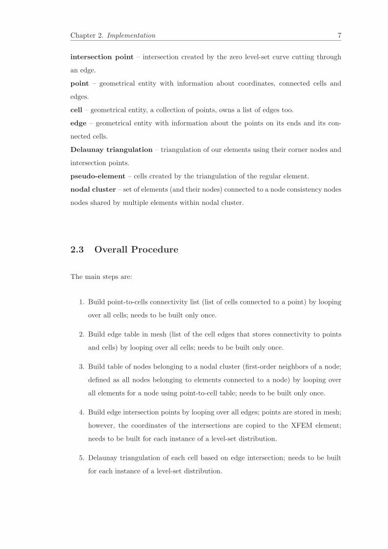
2.3 Overall Procedure
The main steps are:
1. Build point-to-cells connectivity list (list of cells connected to a point) by looping
over all cells; needs to be built only once.
2. Build edge table in mesh (list of the cell edges that stores connectivity to points
and cells) by looping over all cells; needs to be built only once.
3. Build table of nodes belonging to a nodal cluster (first-order neighbors of a node;
defined as all nodes belonging to elements connected to a node) by looping over
all elements for a node using point-to-cell table; needs to be built only once.
4. Build edge intersection points by looping over all edges; points are stored in mesh;
however, the coordinates of the intersections are copied to the XFEM element;
needs to be built for each instance of a level-set distribution.
5. Delaunay triangulation of each cell based on edge intersection; needs to be built
for each instance of a level-set distribution.

Chapter 2. Implementation 8
6. Build table of phases and sub-phases for each triangle/tetrahedron (pseudo-cells)
for each triangulated element; needs to be performed for each instance of level set
distribution.
7. Build enrichment table that defines which nodal degrees of freedom are used to
interpolate a field within a pseudo-element.
8. Determine which degrees of freedom are used in the model.
Figure 2.1: The diagram shows the overall procedure required to implement theXFEM model.
2.4 XFEM Implementation Algorithms
Consider the following XFEM model which consists of a 4-element mesh in 2D; the
nodes on the left are clamped and right edge is subject to a constant pressure load. The
level-set distribution leads to the intersection pattern shown below (figure 2.2). The
mesh below shows the indices of the nodes and the cells (figure 2.3).
2.4.1 Point-to-cells connectivity table
To build a point-to-cell table for each point in our computational mesh we loop over all
base cells in the computational mesh (base cells are all cells that are not side-set cells).
For each base cell we loop over all points and store the current cell index with point
index. This leads to the point-to-cell connectivity table (see table 2.1):

Chapter 2. Implementation 9
Figure 2.2: 4-element 2D mesh. Blue areas: material phase 1 negative level-set valueat the node; red areas: material phase 2, positive level-set value.
Figure 2.3: 4-element 2D mesh. Red numbers represent the Global Element Id, bluenumbers represent the Global Node Id.
Chapter 2. Implementation 10
Point Id Number of cells connected Cell Ids
1 1 1
2 2 1,2
3 4 1,2,3,4
4 2 1,4
5 1 2
6 2 2,3
7 1 3
8 2 3,4
9 1 4
Table 2.1: Point ID to cell IDs connectivity table
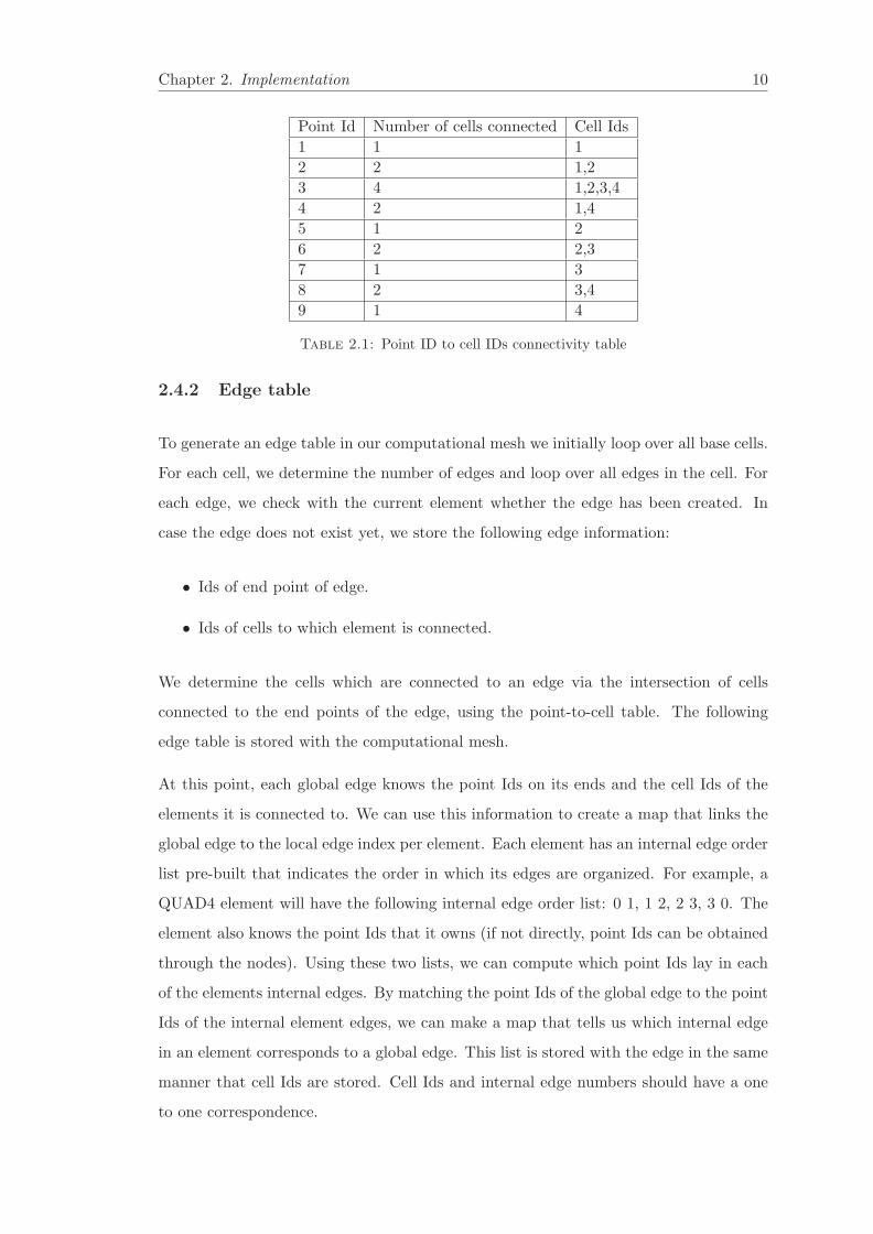
2.4.2 Edge table
To generate an edge table in our computational mesh we initially loop over all base cells.
For each cell, we determine the number of edges and loop over all edges in the cell. For
each edge, we check with the current element whether the edge has been created. In
case the edge does not exist yet, we store the following edge information:
• Ids of end point of edge.
• Ids of cells to which element is connected.
We determine the cells which are connected to an edge via the intersection of cells
connected to the end points of the edge, using the point-to-cell table. The following
edge table is stored with the computational mesh.
At this point, each global edge knows the point Ids on its ends and the cell Ids of the
elements it is connected to. We can use this information to create a map that links the
global edge to the local edge index per element. Each element has an internal edge order
list pre-built that indicates the order in which its edges are organized. For example, a
QUAD4 element will have the following internal edge order list: 0 1, 1 2, 2 3, 3 0. The
element also knows the point Ids that it owns (if not directly, point Ids can be obtained
through the nodes). Using these two lists, we can compute which point Ids lay in each
of the elements internal edges. By matching the point Ids of the global edge to the point
Ids of the internal element edges, we can make a map that tells us which internal edge
in an element corresponds to a global edge. This list is stored with the edge in the same
manner that cell Ids are stored. Cell Ids and internal edge numbers should have a one
to one correspondence.
Chapter 2. Implementation 11
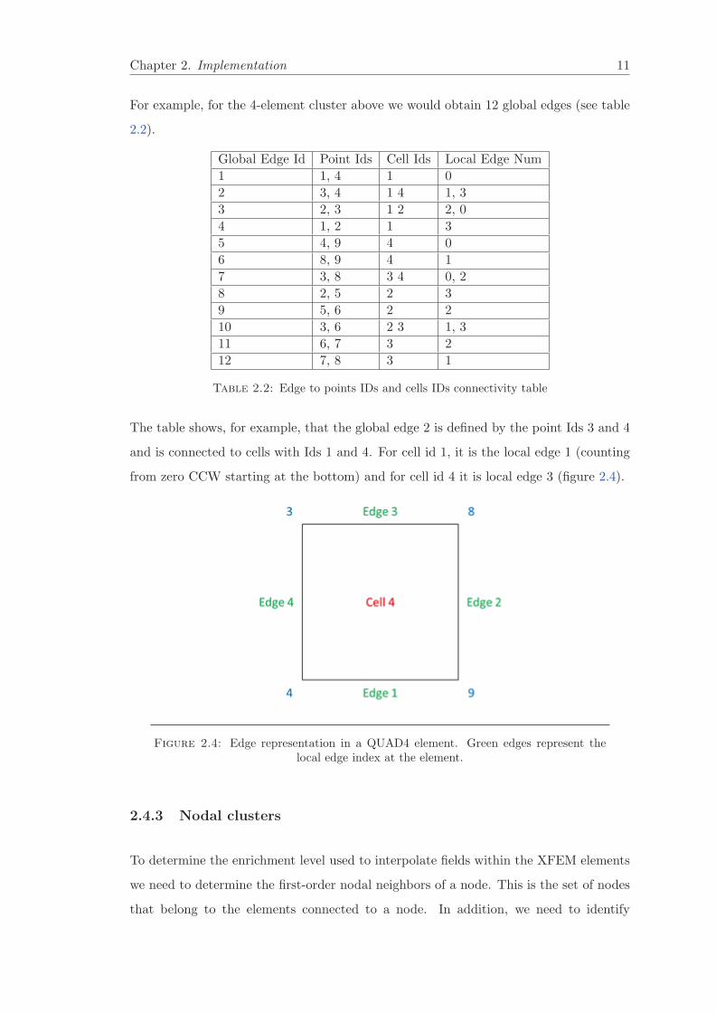
For example, for the 4-element cluster above we would obtain 12 global edges (see table
2.2).
Global Edge Id Point Ids Cell Ids Local Edge Num
1 1, 4 1 0
2 3, 4 1 4 1, 3
3 2, 3 1 2 2, 0
4 1, 2 1 3
5 4, 9 4 0
6 8, 9 4 1
7 3, 8 3 4 0, 2
8 2, 5 2 3
9 5, 6 2 2
10 3, 6 2 3 1, 3
11 6, 7 3 2
12 7, 8 3 1
Table 2.2: Edge to points IDs and cells IDs connectivity table
The table shows, for example, that the global edge 2 is defined by the point Ids 3 and 4
and is connected to cells with Ids 1 and 4. For cell id 1, it is the local edge 1 (counting
from zero CCW starting at the bottom) and for cell id 4 it is local edge 3 (figure 2.4).
Figure 2.4: Edge representation in a QUAD4 element. Green edges represent thelocal edge index at the element.
2.4.3 Nodal clusters
To determine the enrichment level used to interpolate fields within the XFEM elements
we need to determine the first-order nodal neighbors of a node. This is the set of nodes
that belong to the elements connected to a node. In addition, we need to identify

Chapter 2. Implementation 12
the nodes that belong to two or more elements; we refer to these nodes as consistency
nodes. Consistency nodes are simply the nodes in a nodal cluster (nodes of the connected
elements of a main node) that are shared by more than one element in the nodal cluster.
This information can be obtained by looping over the connected elements of a node, and
obtaining the node list for each element.
2.4.4 Determine Intersection points
The intersection points are defined by the zero level-set values. We loop over all edges
defined in the edge table created in Step 2 and compute the intersection points along
the edge using the nodal level-set information of the edge endpoints. The coordinates
of the intersection points are then sent to all elements connected to the edge and stored
in the corresponding XFEM element. (see figure 2.5). NOTE: Since edges only know of
the cells connected to it, we use a cell-to-element map in order to be able to send this
information to the XFEM elements. This is owned by the model.
Figure 2.5: Mapping of intersection point to element.

Chapter 2. Implementation 13
2.4.5 Delaunay triangulation and assignment of main and sub-phases
to pseudo-elements
We loop over all elements in the model and, if intersected, we perform a Delaunay
triangulation, using the corner nodes and the edge intersection points stored with the
elements in Step 3. The Delaunay triangulation requires only the coordinates of the
element corner and edge intersection points. The Delaunay triangulation will return a
list of triangles for 2D or tetrahedrons for 3D problems.
2.4.6 Main phase and sub-phase
We assign a main and sub-phase to each triangle/tetrahedron. The main phase is de-
termined based on the average main-phase value of the pseudo-element. In case the
average is zero, we apply an exception rule (TBD). The sub-phase information is based
on the connectivity of pseudo-elements which belong to the same main phase and is
computed via a flood-fill algorithm. To this end we collect the pseudo-elements into a
pseudo-mesh; each triangulated XFEM element has its own pseudo-mesh which consists
of the points and the connectivity of the pseudo-elements. The main steps (figure 2.6)
of the flood-fill algorithm used are:
• Build edge table for pseudo-elements of current XFEM element, analogue to Step
2.4.2.
• Loop over all elements that have not been assigned a sub-phase:
– Find unprocessed element; recursively find neighbors with same main-phase;
assign lowest unassigned sub-phase to elements found in search process.
For figure 2.6, we would get the list in table 2.3:
We have 6 different triangles generated by Delaunay triangulation. By convention, the
order of the triangles is determined after the triangulation so that all phase 1 ones are
located at the top, followed by the phase 2 triangles. Each triangle is assigned a main
phase and sub-phase (see table 2.3); the assignment is stored, using a one-to-one map
by the XFEM element.

Chapter 2. Implementation 14
Figure 2.6: Sub-phase computation algorithm. Refer to section sec:main-phase-sub-phase for a more detailed description.
Triangle number Main Phase Sub-Phase
1 1 0
2 1 0
3 1 0
4 1 0
5 2 1
6 2 2
Table 2.3: Main-phase and sub-phase table for pseudo-elements.
2.4.7 Nodal enrichments for pseudo-elements
To interpolate fields in the XFEM elements we need to determine which nodal enrich-
ments are used within each pseudo element. The enrichments need to be chosen such
that the interpolations are continuous across adjacent elements within the same main
phase and unique within pseudo elements of the main sub-phase but topologically dis-
connected.
The main concept of the procedure is to clearly separate element-level and node-level
operations. This separation enables the parallelization of the procedure. The first step
is to determine the enrichment levels a particular node will use to interpolate fields in
the triangulated elements with a particular sub-phase. This step is done by looping over
all nodes. The result of this loop is a map that links the sub-phase information of an
element to an enrichment level for each node of the element. In a second step we loop

Chapter 2. Implementation 15
over all elements to update the enrichment levels of pseudo-element based on the map
built previously.
Looping over all nodal clusters, we build the following node-element table. The entries
in the table are the sub-phases at the nodes within each element. The consistency node
numbers are marked by a “C”. Consistency nodes can be identified by nodes which have
entries in more than one column; so they can be identified easily on the fly.
Two conditions, consistency and uniqueness, must be satisfied to ensure the assigned
sub-phases are consistent across the nodal cluster. The consistency condition is satisfied
if all sub-phases in a row are the same. The uniqueness condition is satisfied if the
sub-phase of each set of connected nodes is unique in the cluster.
Nodes/Elements 1 2 3 4
1 14
2 “C” 0 0
3 “C” 15 14 14 15
4 “C” 0 0
5 15
6 “C” 0 0
7 15
8 “C” 0 0
9 14
Table 2.4: Initial node-element table.
The initial node-element table (see table 2.4) shows that the consistency condition is
not satisfied since node 3 is inconsistent. Also, nodes 5 and 7, for example, should be
assigned a unique sub-phase. Therefore the uniqueness condition is also not satisfied.
To ensure both conditions we build a second table and where we iteratively correct the
sub-phase until all conditions are satisfied. Note that the consistency and uniqueness
checks are not needed for a 1 element cluster. The correction procedure is as follows:
1. Initialize a list of all sub-phase possible; mark them as unused; initialize a list of
checked nodes. Mark all nodes as unchecked; build list of consistency nodes.
2. Ensure consistency: Repeat the following steps until all consistency nodes are
checked.

Chapter 2. Implementation 16
• Select node: Start with the center node, which must be a consistency node
(remember that this consistency and uniqueness check will not be applied for
a one-element cluster). Otherwise select the first unchecked consistency node.
• Select sub-phase: Select the lowest unused sub-phase. Mark the selected sub-
phase as used (keep consistency of sub-phase to the respective main phase).
• Identify connected consistency nodes and connected unique nodes:
– For each element to which the selected node belongs, connected nodes
have the same sub-phase as the selected node has for this particular
element. Select the connected nodes which may be either consistency or
unique nodes.
– In order to identify all connected consistency and unique nodes, search
the connected elements for additional connected consistency and unique
nodes.
– The above process requires recursively (a) searching for nodes within
an element with the same sub-phase and (b) identifying elements that
share consistency nodes. Note: the sub-phase id might change between
elements if the sub-phases are not consistent yet for a consistency node.
• Assign sub-phase: Assign the selected sub-phase to all connected nodes iden-
tified in the search process described above. For any value that needs to be
changed, flip sub-phases for that element. Mark connected nodes as checked.
Nodes/Elements 1 2 3 4
1 14 → 15
2 “C” 0 0
3 “C” 15 → 14 14 14 15→ 14
4 “C” 0 0
5 15
6 “C” 0 0
7 15
8 “C” 0 0
9 14→ 15
Table 2.5: Flipping the enrichment levels to keep consistency.
3. Ensure uniqueness: Loop through the remaining unchecked nodes. For each ele-
ment, collect the unique nodes with an unused sub-phase, assign the next unused
sub-phase to these nodes and check the sub-phase as being used. Here nodes 1,

Chapter 2. Implementation 17
5, 7, and 9 are assigned the sub-phase 16, 17, and 18, respectively (node 1 was
flipped initially, but it was not marked as checked). The outcome of the above
correction procedure is table 2.6:
Nodes/Elements 1 2 3 4
1 15
2 “C” 0 0
3 “C” 14 14 14 14
4 “C” 0 0
5 16
6 “C” 0 0
7 17
8 “C” 0 0
9 18
Table 2.6: The result of the enrichment algorithm. Nodes that are shared acrosselements receive the same enrichment level.
4. Using the original and the corrected node-element tables we can build the map
for the central point (here node ID 3). See table 2.7. The rows correspond to
the elements, the columns list the original sub-phases, and the entries are the
enrichment levels used by the central node. When building this table we check that
the map is consistent within itself (the same sub-phases within each are assigned
to the same enrichments).
For Node 3: 0 14 15Element / Enrichment level
1 0 15 14
2 0 14 16
3 0 14 17
4 0 18 14
Table 2.7: Element to enrichment table for node ID 3. This table shows the initialenrichments node 3 received during the sub-phase algorithm and the enrichment levels
after the enrichment algorithm.
5. With this map we can loop over all elements and assign enrichment levels for each
node to each pseudo-element, based on their sub-phase information.
2.4.8 Determine degrees of freedom used
The last step in the algorithm is to flag which enrichment levels each node will use for
interpolation. For example, in our test case, node 3 will have enrichment levels 0, 14,

Chapter 2. Implementation 18
15, 16, 17, 18 active.
2.4.9 Implementation Example 2
Figure 2.7: XFEM implementation configuration 2
Nodes/Elements 1 2 3 4
1 0
2 “C” 14 14
3 “C” 0 0 0 0
4 “C” 0 0
5 14
6 “C” 14 14
7 14
8 “C” 14 14
9 0
Table 2.8: Initial node-element table for configuration 2.

Chapter 2. Implementation 19
Nodes/Elements 1 2 3 4
1 0
2 “C” 14 14
3 “C” 0 0 0 0
4 “C” 0 0
5 14
6 “C” 14 14
7 14
8 “C” 14 14
9 0
Table 2.9: Final node-element table for configuration 2.
For Node 3: 0 14
Element / Enrichment level
1 0 14
2 0 14
3 0 14
4 0 14
Table 2.10: Enrichment level map for configuration 2.
2.4.10 Implementation Example 3
Figure 2.8: XFEM implementation configuration 3

Chapter 2. Implementation 20
Nodes/Elements 1 2 3 4
1 0
2 “C” 15 14
3 “C” 0 0 0 0
4 “C” 14 0
5 14
6 “C” 14 14
7 14
8 “C” 14 15
9 0
Table 2.11: Initial node-element table for configuration 3.
Nodes/Elements 1 2 3 4
1 0
2 “C” 14 14
3 “C” 0 0 0 0
4 “C” 15 15
5 14
6 “C” 14 14
7 14
8 “C” 14 14
9 0
Table 2.12: Final node-element table for configuration 3.
For Node 3: 0 14 15
Element / Enrichment level
1 0 15 14
2 0 14
3 0 14
4 0 15 14
Table 2.13: Enrichment level map for configuration 3.

Chapter 2. Implementation 21
2.5 Solving the problem
In the previous section, our algorithms determined which additional enriched degrees
of freedom each node requires to account for the discontinuities in the elements. Once
this is achieved, we can proceed to solve our problem like a regular FEM problem
because in the end, the enriched degrees of freedom are just that, degrees of freedom
like displacement or stress.
The only difference comes in which functions are used to interpolate. The original
degrees of freedom are interpolated using the regular shape functions for the problem.
The enriched degrees of freedom will interpolate using shape functions based on the
partition of unity and the Heaviside function.
A standard extended finite element approximation of a function u(x) is:
uh(x) =∑i∈I
Ni(x)ui +∑i∈I∗
Mi(x)ai (2.1)
The first sum is the standard FEM approximation while the second sum is the enrichment
applied to the interpolation.
In this function, the domain Ω ∈ Rn is n − dimensional and it is meshed into nel
elements. The other terms mean:
uh(x) – approximated function.
Ni(x) – standard FE shape function at node i.
ui – solution for the displacement at node i.
I – set of all nodes in the domain.
Mi(x) – local enrichment function at node i.
ai – displacement of the enriched displacement at node i.
I∗ – set of all enriched nodes ∈ I.
The enrichment functions are built by means of the partition of unity principle.
Mi(x) = N∗i (x) ∗Ψ(x) (2.2)

Chapter 2. Implementation 22
where N∗i (x) are the partition of unity functions such that
∑i∈I∗
N∗i (x) = 1 (2.3)
The implementation in this document models weak discontinuities and therefore, the
global enrichment function is chosen based on the Heaviside function as follows:
ψ(x) = sign(φ(x)) =
⎧⎪⎪⎪⎨⎪⎪⎪⎩
−1 if φ(x) < 0
0 if φ(x) = 0
1 if φ(x) > 0
(2.4)
2.6 Preconditioner
When a sub-domain of a material phase is too small (around O(ε1/2)), the Jacobian
matrix will be ill-conditioned. To solve this shortcoming, it is necessary to scale the
matrix with another pre-conditioning matrix. This scaling matrix will be a function of
the level-set field.
The pre-conditioner will have a scaling value for each degree of freedom in the problem.
If the degree of freedom is constrained, the scaling value will be 1. To obtain these
values, we check which enriched degrees of freedom each node uses. Then, proceed to
compute the integral of the shape function for the node with respect to the material sub-
domain that requires said enriched degree of freedom. Because a node will have different
scaling values across multiple elements, there are four pre-conditioner implementations
available to compute the scaling value in a nodal cluster:
• Maximum value of integrals of shape functions
• Sum of values of integrals of shape functions
• Maximum value of integrals of the derivatives of the shape functions
• Sum of values of integrals of the derivatives of the shape functions

Chapter 2. Implementation 23
After this computation, each node will have a scaling value for each enriched degree of
freedom it is using. This scaled value is computed as the inverse of the square root of
the integral calculated.
At this point, there is one scaling value for each degree of freedom in the system. These
scaling values are applied to the solution vector before the computation of the residual
and Jacobian. After the residual and Jacobian are computed, they are both unscaled
and then the new solution vector is computed.

Chapter 3
XFEM corroboration and results
3.1 Methodology
Two formulations were used to corroborate the results of the XFEM implementation.
Equation 3.1 computes the difference in solutions at the discontinuity. Since the model
we have implemented is based on inclusions and not crack propagation, this interface
error should approach zero as the mesh gets finer.
√∑element
∑interface
∫u+ − u−dΓi∑
element
∑interface
∫dΓi
(3.1)
This equation computes the interface “jump” across all interfaces and elements in the
model, then scales it with respect to the perimeter or area of the interface, and finally
takes the square root.
Equation 3.2 compares the relative difference between the XFEM solution and the FEM
solution.
√∫uXFEM − uFEMdΩ∫
uFEMdΩ(3.2)
uXFEM represents the XFEM solution, while uFEM represents the FEM solution.
24

Chapter 3. Results 25
XFEM was used to solve a thermal problem with the configuration of figure 3.1. The
same problem was ran using the classical FEM. The FEM problem used two different
types of elements and its mesh was refined until the solution reached convergence.
Figure 3.1: Thermal problem setup.
The mesh has a width of 20 units and a height of 20 units. The problem has Dirichlet
boundary conditions on the sides. The temperature is prescribed to 0 on the left side and
100 on the right side. There is an inclusion at the center of the model. This inclusion
is a different material with a different thermal conductivity than the material phase 1
domain.
The test consisted in modifying the diameter of the circle from 2 units to 6 units in
500 steps using different mesh refinements, different conductivity ratios and different
pre-conditioners formulations.
3.2 Tests
3.2.1 Mesh refinement sweep
The mesh size was the variable in this test, while the conductivity ratio between both
materials remained fixed at 10. No pre-conditioner scaling was applied. The different

Chapter 3. Results 26
mesh sizes used were:
• 20x20
• 30x30
• 40x40
• 50x50
Figure 3.2 shows that as the mesh is refined, the interface error converges to zero.
Figure 3.2: Mesh refinement sweep interface error.
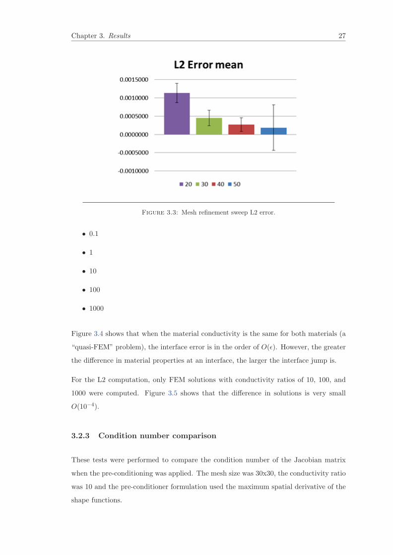
Figure 3.3 shows that as the mesh is refined, the difference of the XFEM solution with
respect to the FEM solution decreases. The larger difference for the 50x50 mesh is due
to the sampling and different mesh sizes used for the XFEM and FEM problems. A
different mesh resampling size fixed the issue in other tests.
3.2.2 Conductivity ratio sweep
The conductivity ratio between the different materials was the variable in this test. The
mesh size was 30x30 and the pre-conditioner formulation used the maximum spatial
derivative of the shape functions. The different conductivity ratios used were:
Chapter 3. Results 27
Figure 3.3: Mesh refinement sweep L2 error.
• 0.1
• 1
• 10
• 100
• 1000
Figure 3.4 shows that when the material conductivity is the same for both materials (a
“quasi-FEM” problem), the interface error is in the order of O(ε). However, the greater
the difference in material properties at an interface, the larger the interface jump is.
For the L2 computation, only FEM solutions with conductivity ratios of 10, 100, and
1000 were computed. Figure 3.5 shows that the difference in solutions is very small
O(10−4).
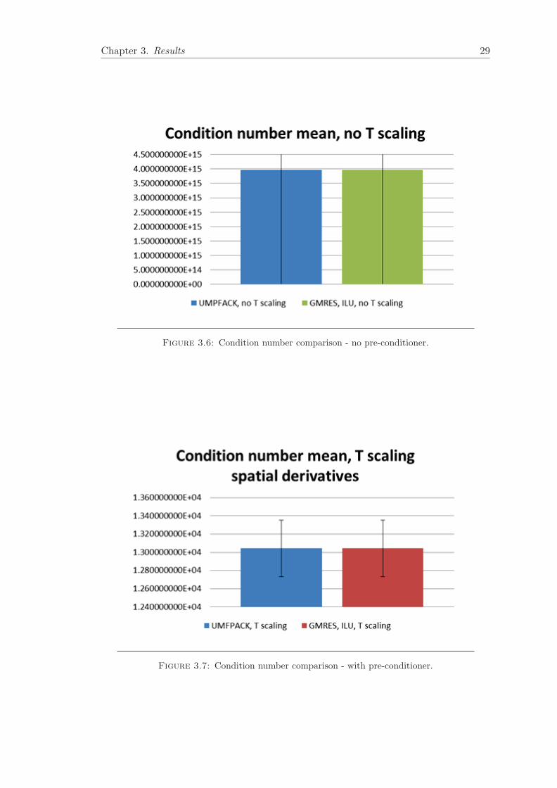
3.2.3 Condition number comparison
These tests were performed to compare the condition number of the Jacobian matrix
when the pre-conditioning was applied. The mesh size was 30x30, the conductivity ratio
was 10 and the pre-conditioner formulation used the maximum spatial derivative of the
shape functions.

Chapter 3. Results 28
Figure 3.4: Conductivity refinement sweep interface error.
Figure 3.5: Conductivity refinement sweep L2 error.
Two different solution algorithms were used and compared, a direct solver and a GMRES
iterative solver.
Figure 3.6 shows that the Jacobian matrix has a condition number in the order of 1015
when no pre-conditioning is applied, while figure 3.7 shows that condition number is
decreased to the order of 104 when scaling is applied.
Chapter 3. Results 29
Figure 3.6: Condition number comparison - no pre-conditioner.
Figure 3.7: Condition number comparison - with pre-conditioner.

Chapter 4
Conclusions and Future Work
4.1 Conclusions
The framework developed in this project will help eliminate the need to re-mesh a model
when discontinuities present in the domain. The program is capable of dividing an el-
ement into integrable sub-domains, calculating its topology, its enrichment information
and computing the normal vector and Gauss points required for integration. The pro-
gram is also capable of solving XFEM problems with different topologies in 3D.
Results showed that the differences in solutions with a classical FEM problem are small.
XFEM produced Jacobian matrices with high condition numbers, but the application
of a pre-conditioner as a function of the level-set field solved this shortcoming.
4.2 Future Work
Future work in this project involves the implementation of the algorithms in a parallel
environment. The framework for a parallel algorithm would include two intermediate
steps: one between the sub-phase computation and the enrichment level computation
and another after the enrichment level algorithm and before the solution of the problem.
The first exchange would communicate sub-phase information from elements connected
to a node across separate processors. The second exchange of information would send and
receive the different enriched degrees of freedom across elements on multiple processors.
30

Chapter 4. Conclusions and future work 31
This last exchange would follow the rules of classical parallel FEM code for coupled
problems where two elements have different degrees of freedom.

Appendix A
Delaunay Triangulation code
This code written in Matlab is the first attempt of the author to perform a Delaunay
triangulation in an element based on the level-set function values at the corner nodes.
To triangulate different discontinuity configurations change the levs variable: each entry
corresponds to the value of the level-set function at a node. The ex, ey and ez vector
variables contain the coordinates of the corner nodes and can be modified to change the
shape of the element.
A.1 main.m
1 function [] = main()
2 % Main program
3 % Modify ex , ey , and ez to change shape of element
4 % Change levs to change level -set configuration
5
6 % Global x,y,z coordinates of element.
7 % This will form a 3D cubic element cube.
8 ex = [-0.5 -0.5 -0.5 -0.5 0.5 0.5 0.5 0.5];
9 ey = [-0.5 -0.5 0.5 0.5 -0.5 -0.5 0.5 0.5];
10 ez = [0.5 -0.5 -0.5 0.5 0.5 -0.5 -0.5 0.5];
11
12 %% Extract a particular case (set k manually).
13
14 % Initial test for a particular levelset function.
15 % Randn function will return a m x n matrix of random positive and negative
16 % numbers.
17 hexsect = cell (127 ,8);
18 k = round(1 + (127 -1).*rand);
32
Appendix A. Delaunay triangulation 33
19 % levs = randn (1 ,8);
20 levs = [-1 -1 -1 -1 -1 -1 -1 1];
21 % levs = [-10 1 -10 1 -10 1 -10 1];
22 [nsct ,isct ,xsct ,ysct ,zsct ,levs] = xfem8isct(ex ,ey ,ez ,levs);
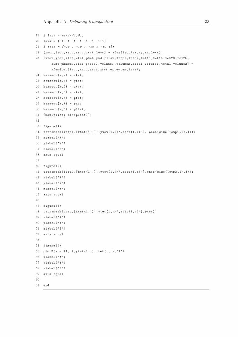
23 [xtet ,ytet ,ztet ,ctet ,ptet ,pnd ,plist ,Tetp1 ,Tetp2 ,tet1G ,tet1L ,tet2G ,tet2L ,
size_phase1 ,size_phase2 ,volume1 ,volume2 ,total_volume1 ,total_volume2] =
xfem8tet(isct ,xsct ,ysct ,zsct ,ex,ey,ez ,levs);
24 hexsect{k,2} = xtet;
25 hexsect{k,3} = ytet;
26 hexsect{k,4} = ztet;
27 hexsect{k,5} = ctet;
28 hexsect{k,6} = ptet;
29 hexsect{k,7} = pnd;
30 hexsect{k,8} = plist;
31 [max(plist) min(plist)];
32
33 figure (1)
34 tetramesh(Tetp1 ,[xtet (1,:) ’,ytet (1,:) ’,ztet (1,:) ’],-ones(size(Tetp1 ,1) ,1));
35 xlabel(’X’)
36 ylabel(’Y’)
37 zlabel(’Z’)
38 axis equal
39
40 figure (2)
41 tetramesh(Tetp2 ,[xtet (1,:) ’,ytet (1,:) ’,ztet (1,:) ’],ones(size(Tetp2 ,1) ,1));
42 xlabel(’X’)
43 ylabel(’Y’)
44 zlabel(’Z’)
45 axis equal
46
47 figure (3)
48 tetramesh(ctet ,[xtet (1,:) ’,ytet (1,:) ’,ztet (1,:) ’],ptet);
49 xlabel(’X’)
50 ylabel(’Y’)
51 zlabel(’Z’)
52 axis equal
53
54 figure (4)
55 plot3(xtet (1,:),ytet (1,:),ztet (1,:),’X’)
56 xlabel(’X’)
57 ylabel(’Y’)
58 zlabel(’Z’)
59 axis equal
60
61 end

Appendix A. Delaunay triangulation 34
A.2 xfem8isct.m
1 function [nsct ,isct ,xsct ,ysct ,zsct ,levs] = xfem8isct(ex ,ey ,ez ,levs)
2
3 % Intersection of hex8 based on level -set values.
4 %
5 % Input: ex : global x- coordinates of nodes of 3D element
6 % ey : global y- coordinates of nodes of 3D element
7 % ez : global z- coordinates of nodes of 3D element
8 % levs : level set values randomly generated
9 %
10 % Output: nsct : number of intersected edges
11 % isect : vector flags of intersected edges
12 % xsect : x- coordinates of intersections in global and local coordinates
13 % ysect : y- coordinates of intersections in global and local coordinates
14 % zsect : z- coordinates of intersections in global and local coordinates
15
16 % Map of node connections across edges in a 3D element.
17 % Edgmap is a 12 x 2 matrix.
18 edgmap = [ 1 2; 2 3; 3 4; 4 1; 1 5; 2 6; 3 7; 4 8; 5 6; 6 7; 7 8; 8 5];
19
20 % Values of nodes in master element (local coordinates ).
21
22 xp = [-1 -1 -1 -1 1 1 1 1];
23 yp = [-1 -1 1 1 -1 -1 1 1];
24 zp = [1 -1 -1 1 1 -1 -1 1];
25
26 % Set initial value of intersected edges to zero.
27 % Create a zero 12 x 1 matrix to flag edges with intersected edges.
28 % Create a zero 12 x 2 matrix to record x, y, z coordinates in global and
29 % local coordinates .
30 nsct = 0;
31 isct = zeros (12 ,1);
32 xsct = zeros (12 ,2);
33 ysct = zeros (12 ,2);
34 zsct = zeros (12 ,2);
35
36 for i = 1:12
37 % ic1 and ic2 return the values of the first and second columns of
38 % edgmap , respectively , for a determined row. ic1 and ic2 represent two
39 % nodes connected by a cube edge.
40 ic1 = edgmap(i,1);
41 ic2 = edgmap(i,2);
42 % The level set values at those nodes are multiplied to determined
43 % intersection .
44 if levs(ic1)*levs(ic2) < 0 % If so , then there is an intersection .
45 nsct = nsct +1; % Increase number of intersected edges by one
.
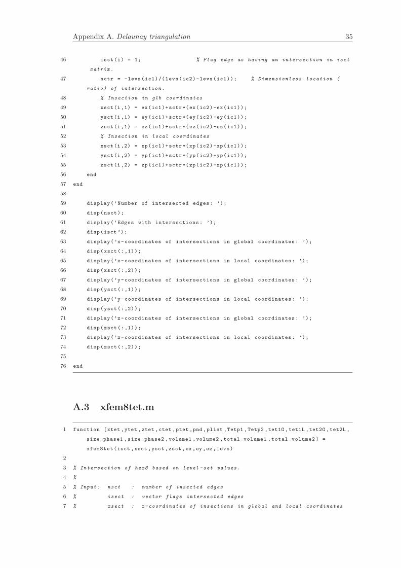
Appendix A. Delaunay triangulation 35
46 isct(i) = 1; % Flag edge as having an intersection in isct
matrix.
47 sctr = -levs(ic1)/(levs(ic2)-levs(ic1)); % Dimensionless location (
ratio) of intersection .
48 % Insection in glb coordinates
49 xsct(i,1) = ex(ic1)+sctr*(ex(ic2)-ex(ic1));
50 ysct(i,1) = ey(ic1)+sctr*(ey(ic2)-ey(ic1));
51 zsct(i,1) = ez(ic1)+sctr*(ez(ic2)-ez(ic1));
52 % Insection in local coordinates
53 xsct(i,2) = xp(ic1)+sctr*(xp(ic2)-xp(ic1));
54 ysct(i,2) = yp(ic1)+sctr*(yp(ic2)-yp(ic1));
55 zsct(i,2) = zp(ic1)+sctr*(zp(ic2)-zp(ic1));
56 end
57 end
58
59 display(’Number of intersected edges: ’);
60 disp(nsct);
61 display(’Edges with intersections: ’);
62 disp(isct ’);
63 display(’x-coordinates of intersections in global coordinates: ’);
64 disp(xsct (:,1));
65 display(’x-coordinates of intersections in local coordinates: ’);
66 disp(xsct (:,2));
67 display(’y-coordinates of intersections in global coordinates: ’);
68 disp(ysct (:,1));
69 display(’y-coordinates of intersections in local coordinates: ’);
70 disp(ysct (:,2));
71 display(’z-coordinates of intersections in global coordinates: ’);
72 disp(zsct (:,1));
73 display(’z-coordinates of intersections in local coordinates: ’);
74 disp(zsct (:,2));
75
76 end
A.3 xfem8tet.m
1 function [xtet ,ytet ,ztet ,ctet ,ptet ,pnd ,plist ,Tetp1 ,Tetp2 ,tet1G ,tet1L ,tet2G ,tet2L ,
size_phase1 ,size_phase2 ,volume1 ,volume2 ,total_volume1 ,total_volume2] =
xfem8tet(isct ,xsct ,ysct ,zsct ,ex,ey,ez ,levs)
2
3 % Intersection of hex8 based on level -set values.
4 %
5 % Input: nsct : number of insected edges
6 % isect : vector flags intersected edges
7 % xsect : x- coordinates of insections in global and local coordinates

Appendix A. Delaunay triangulation 36
8 % ysect : y- coordinates of insections in global and local coordinates
9 % zsect : z- coordinates of insections in global and local coordinates
10 % ex : global x- coordinates of nodes
11 % ey : global y- coordinates of nodes
12 % ez : global z- coordinates of nodes
13 % levs : levs
14 %
15 % Output: xtet : x- coordinates of nodes of triangulated element
16 % ytet : y- coordinates of nodes of triangulated element
17 % ztet : z- coordinates of nodes of triangulated element
18 % ctet : connectivity of tets in triangulated element
19 % ptet : phase of each tetrahedron
20 % pnd : nodal levelset values (actual values), # of nodes
21 % plist : phase of each node (in terms of -1, 1 and 0)
22 % Tetp1 : nodes of tetrahedrons for main phase 1
23 % Tetp2 : nodes of tetrahedrons for main phase 2
24 % tet1G : global coordinates of tetrahedron for phase 1
25 % tet1L : local coordinates of tetrahedron for phase 1
26 % tet2G : global coordinates of tetrahedron for phase 1
27 % tet2L : local coordinates of tetrahedron for phase 2
28 % size_phase1 : number of tetrahedrons in phase 1
29 % size_phase2 : number of tetrahedrons in phase 2
30 % volume1 : volume of a tetrahedron in phase 1
31 % volume2 : volume of a tetrahedron in phase 2
32 % total_volume1 : total volume of all tetrahedrons in phase 1
33 % total_volume2 : total volume of all tetrahedrons in phase 2
34
35 %% Identify coordinates and phases to triangulate
36
37 % Nodes in local coordinates
38 xp = [-1 -1 -1 -1 1 1 1 1];
39 yp = [-1 -1 1 1 -1 -1 1 1];
40 zp = [1 -1 -1 1 1 -1 -1 1];
41
42 % Find intersected edges. Order of edges depends on configuration of edgmap
43 % isct flagged intersected edges with a 1
44 itr = find(isct >0);
45 % Sort nodes by main phase. Determine which nodes have positive or negative
46 % level -set values.
47 ip1 = find(levs <0);
48 ip2 = find(levs >0);
49
50 % Id -numbers of node at edge intersections , i.e. create pseudonodes
51 ips = 9:8+ length(itr);
52
53 % Create phase vector for triangulated element. Vector contains level -set
54 % values at the 8 original nodes plus zero values for the new pseudonodes
55 pnd = [levs zeros(1,length(itr))];

Appendix A. Delaunay triangulation 37
56
57 % Create nodes for main phase 1
58 % Coordinates where nodes are negative plus coordinates of intersections in
59 % global coordinates
60 exp1 = [ex(ip1) xsct(itr ,1) ’];
61 eyp1 = [ey(ip1) ysct(itr ,1) ’];
62 ezp1 = [ez(ip1) zsct(itr ,1) ’];
63 % Nodes and pseudonodes numbers of main phase 1
64 ipx1 = [ip1 ips];
65
66 % Create nodes for main phase 2
67 % Coordinates where nodes are positive plus coordinates of intersections in
68 % global coordinates
69 exp2 = [ex(ip2) xsct(itr ,1) ’];
70 eyp2 = [ey(ip2) ysct(itr ,1) ’];
71 ezp2 = [ez(ip2) zsct(itr ,1) ’];
72 % Nodes and pseudonodes numbers of main phase 2
73 ipx2 = [ip2 ips];
74
75 % Combine triangulation points of main phase 1 and 2 in local and global
76 % coordinates
77 xtet = [ex xsct(itr ,1) ’;xp xsct(itr ,2) ’];
78 ytet = [ey ysct(itr ,1) ’;yp ysct(itr ,2) ’];
79 ztet = [ez zsct(itr ,1) ’;zp zsct(itr ,2) ’];
80
81 % Same as xtet , ytet , ztet , but only with global coordinates . Useful for
82 % triangulation below.
83 exp = [ex xsct(itr ,1) ’];
84 eyp = [ey ysct(itr ,1) ’];
85 ezp = [ez zsct(itr ,1) ’];
86
87 %% Triangulate main phase 1 and 2 together
88 % If we triangulate main phase 1 and 2 separately , tetrahedron will
89 % superpose for some level -set combinations . We need to triangulate the
90 % entire element as a whole.
91
92 Tp = DelaunayTri(exp ’,eyp ’,ezp ’);
93 Tetp = Tp.Triangulation (:,:);
94
95 %% Separate triangulation into main phases 1 and 2
96
97 Tetp1 = zeros (1,4);
98 Tetp2 = zeros (1,4);
99 index1 = 1;
100 index2 = 1;
101 % If tetrahedron contains a negative node , it is phase 1. Phase 2,
102 % otherwise .
103 for i = 1:size(Tetp ,1)

Appendix A. Delaunay triangulation 38
104 if pnd(Tetp(i,1)) < 0|| pnd(Tetp(i,2)) < 0|| pnd(Tetp(i,3)) < 0|| pnd(Tetp(i
,4)) < 0
105 Tetp1(index1 ,:) = Tetp(i,:);
106 index1 = index1 + 1;
107 else
108 Tetp2(index2 ,:) = Tetp(i,:);
109 index2 = index2 +1;
110 end
111 end
112
113 %% Display coordinates of phase 1 tetrahedrons
114 % Display coordinates of phase 1 tetrahedrons in global coordinates
115 % Display volume of each phase 1 tetrahedron
116 total_volume1 = 0;
117 display(’The global coordinates for the phase 1 tetrahedrons are: ’)
118 for i = 1:size(Tetp1 ,1)
119 tet1G = [xtet(1,Tetp1(i,1)),ytet(1,Tetp1(i,1)),ztet(1,Tetp1(i,1));xtet(1,
Tetp1(i,2)),ytet(1,Tetp1(i,2)),ztet(1,Tetp1(i,2));xtet(1,Tetp1(i,3)),ytet(1,
Tetp1(i,3)),ztet(1,Tetp1(i,3));xtet(1,Tetp1(i,4)),ytet(1,Tetp1(i,4)),ztet(1,
Tetp1(i,4))];
120 disp(tet1G)
121 % Calculate volume. Algorithm : For 4 points in tetrahedron P,Q,R,S,
122 % volume = abs(det ([Q-P;R-Q;S-R]))/6
123 a = tet1G (2,:)-tet1G (1,:);
124 b = tet1G (3,:)-tet1G (2,:);
125 c = tet1G (4,:)-tet1G (3,:);
126 volume1 = abs(det([a;b;c]))/6;
127 total_volume1 = total_volume1 + volume1;
128 display(’The volume of phase 1 tetrahedron is: ’)
129 disp(volume1)
130 end
131
132 % Display coordinates of phase 1 tetrahedrons in local coordinates
133 display(’The local coordinates for the phase 1 tetrahedrons are: ’)
134 for i = 1:size(Tetp1 ,1)
135 tet1L = [xtet(2,Tetp1(i,1)),ytet(2,Tetp1(i,1)),ztet(2,Tetp1(i,1));xtet(2,
Tetp1(i,2)),ytet(2,Tetp1(i,2)),ztet(2,Tetp1(i,2));xtet(2,Tetp1(i,3)),ytet(2,
Tetp1(i,3)),ztet(2,Tetp1(i,3));xtet(2,Tetp1(i,4)),ytet(2,Tetp1(i,4)),ztet(2,
Tetp1(i,4))];
136 disp(tet1L)
137 end
138
139 % Display total volume of phase 1 tetrahedrons
140 display(’The total volume of phase 1 tetrahedrons is: ’)
141 disp(total_volume1)
142
143 %% Display coordinates of phase 2 tetrahedrons
144 % Display coordinates of phase 2 tetrahedrons in global coordinates

Appendix A. Delaunay triangulation 39
145 % Display volume of each phase 2 tetrahedron
146 total_volume2 = 0;
147 display(’The global coordinates for the phase 2 tetrahedrons are: ’)
148 for i = 1:size(Tetp2 ,1)
149 tet2G = [xtet(1,Tetp2(i,1)),ytet(1,Tetp2(i,1)),ztet(1,Tetp2(i,1));xtet(1,
Tetp2(i,2)),ytet(1,Tetp2(i,2)),ztet(1,Tetp2(i,2));xtet(1,Tetp2(i,3)),ytet(1,
Tetp2(i,3)),ztet(1,Tetp2(i,3));xtet(1,Tetp2(i,4)),ytet(1,Tetp2(i,4)),ztet(1,
Tetp2(i,4))];
150 disp(tet2G)
151 % Calculate volume.
152 a = tet2G (2,:)-tet2G (1,:);
153 b = tet2G (3,:)-tet2G (2,:);
154 c = tet2G (4,:)-tet2G (3,:);
155 volume2 = abs(det([a;b;c]))/6;
156 total_volume2 = total_volume2 + volume2;
157 display(’The volume of phase 2 tetrahedron is: ’)
158 disp(volume2)
159 end
160
161 % Display coordinates of phase 2 tetrahedrons in local coordinates
162 display(’The local coordinates for the phase 2 tetrahedrons are: ’)
163 for i = 1:size(Tetp2 ,1)
164 tet2L = [xtet(2,Tetp2(i,1)),ytet(2,Tetp2(i,1)),ztet(2,Tetp2(i,1));xtet(2,
Tetp2(i,2)),ytet(2,Tetp2(i,2)),ztet(2,Tetp2(i,2));xtet(2,Tetp2(i,3)),ytet(2,
Tetp2(i,3)),ztet(2,Tetp2(i,3));xtet(2,Tetp2(i,4)),ytet(2,Tetp2(i,4)),ztet(2,
Tetp2(i,4))];
165 disp(tet2L)
166 end
167
168 % Display total volume of phase 2 tetrahedrons
169 display(’The total volume of phase 2 tetrahedrons is: ’)
170 disp(total_volume2)
171
172 %% Display number of tetrahedrons in each phase.
173 size_phase1 = size(Tetp1 (:,1));
174 size_phase1 = size_phase1 (1);
175 size_phase2 = size(Tetp2 (:,1));
176 size_phase2 = size_phase2 (1);
177 display(’The number of tetrahedrons in phase 1 is: ’)
178 disp(size_phase1);
179 display(’The number of tetrahedrons in phase 2 is: ’)
180 disp(size_phase2);
181
182 %% Locate triangle interfaces - new algorithm
183 % Use function ismember to compare array vectors
184 % Display only result if three nodes repeat
185
186 display(’The interfaces can be found on the triangles with nodes: ’)

Appendix A. Delaunay triangulation 40
187 for i = 1:size(Tetp1 ,1)
188 for j = 1:size(Tetp2 ,1)
189 r = ismember(Tetp1(i,:),Tetp2(j,:));
190 Tetp1_tri = Tetp1(i,:);
191 Tetp1_tri = Tetp1_tri(r);
192 if size(Tetp1_tri ,2) == 3
193 disp(Tetp1_tri)
194 end
195 end
196 end
197
198 %% Combine triangulation of nodes in ctet
199 % Size of ptet depends on number of tetrahedrons
200 % Phase 1 tetrahedrons have value of -1, phase 2 value of 1 in ptet
201
202 % Original:
203 % ctet =[ Tetp1;Tetp2 ];
204 % ptet=[-ones(size(Tetp1 ,1) ,1);ones(size(Tetp2 ,1) ,1)];
205
206 % New method:
207 % Provide two options for triangulation
208 % Option 1: based on volume
209 % If one phase is significantly larger than the other , switch tetramesh
210 if total_volume2 <= (0.2*( total_volume1 + total_volume2))
211 ctet=[ Tetp2;Tetp1];
212 ptet=[-ones(size(Tetp2 ,1) ,1);ones(size(Tetp1 ,1) ,1)];
213 else
214 ctet=[ Tetp1;Tetp2];
215 ptet=[-ones(size(Tetp1 ,1) ,1);ones(size(Tetp2 ,1) ,1)];
216 end
217
218 % Option 2: based on user ’s choice
219 % option = input(’Choose triangulation option 1 or 2: ’);
220 % if option == 1
221 % ctet =[ Tetp2;Tetp1 ];
222 % ptet=[-ones(size(Tetp2 ,1) ,1);ones(size(Tetp1 ,1) ,1)];
223 % elseif
224 % ctet =[ Tetp1;Tetp2 ];
225 % ptet=[-ones(size(Tetp1 ,1) ,1);ones(size(Tetp2 ,1) ,1)];
226 % end
227
228 %% Check connectivity between phases. PART of ORIGINAL CODE
229
230 % Obsolete? plist produces the same value as pnd
231 % Check connectivity for main phase 1 and creat sub -phase information
232
233 % Matrix plisp1 formed of (nodes + pseudonodes ) x 1 elements with value of
234 % -2. ipx1 represents location of phase 1 nodes + pseudonodes . At these

Appendix A. Delaunay triangulation 41
235 % locations , values are replaced by -1
236 plisp1 = -2*ones(size(xtet ,2) ,1);
237 plisp1(ipx1) = -1;
238
239 domp1 = 0;
240 % While there are phase 1 nodes
241 while ismember(-1,plisp1) > 0
242 domp1 = domp1 + 1;
243 % Find where the negative nodes are in the nodes + pseudonodes vector
244 % Value are progressively changed by 0, one at a time
245 ppp = find(plisp1 == -1);
246 plisp1(ppp (1)) = 0;
247 % Locate where values were changed to zero and create new variable ppp
248 % pid represents the node where value has transformed into zero
249 while ismember(0,plisp1) > 0
250 ppp = find(plisp1 == 0);
251 pid = ppp (1);
252 for it = 1:size(ctet ,1)
253 % If the node at pid belongs to Tetp1 and is negative
254 if ismember(pid ,ctet(it ,:)) > 0 && ptet(it) < 0
255 plisp1(ctet(it ,:)) = max(0,plisp1(ctet(it ,:)));
256 end
257 end
258 % At the location of phase 1 nodes + pseudonodes , the value will be
259 % replaced to 1.
260 plisp1(pid) = domp1;
261 end
262 end
263
264 % Check connectivity for main phase 2 and creat sub -phase information
265 % Functions the same as previous routine , but for phase 2
266 plisp2 = -2*ones(size(xtet ,2) ,1);
267 plisp2(ipx2) = -1;
268
269 domp2 = 0;
270 while ismember(-1,plisp2) > 0
271 domp2 = domp2 +1;
272 ppp = find(plisp2 == -1);
273 plisp2(ppp (1)) = 0;
274 while ismember(0,plisp2) > 0
275 ppp = find(plisp2 == 0);
276 pid = ppp (1);
277 for it = 1:size(ctet ,1)
278 if ismember(pid ,ctet(it ,:)) > 0 && ptet(it) > 0
279 plisp2(ctet(it ,:)) = max(0,plisp2(ctet(it ,:)));
280 end
281 end
282 plisp2(pid) = domp2;

Appendix A. Delaunay triangulation 42
283 end
284 end
285
286 % Build phase list including subphase information
287 % Replace all pseudonodes by 0
288 plisp1(ips) = 0;
289 plisp2(ips) = 0;
290
291 % Find location of the pseudonodes
292 idp1 = find(plisp1 >0);
293 idp2 = find(plisp2 >0);
294
295 % Create a zero (nodes + pseudonodes ) x 1 matrix plist
296 plist = zeros(size(xtet ,2) ,1);
297 % Create list that shows which original nodes belong to phase I and II
298 plist(idp1) = -plisp1(idp1);
299 plist(idp2) = plisp2(idp2);
300
301 end
A.4 number configurations.m
1 function [] = number_configurations ()
2 % This function computes all possible combinations of level -set function
3 % values at the corner nodes to obtain the number of 3D triangulation
4 % combinations possible.
5
6 % x,y,z coordinates of element.
7 % This will form a 3D cubic element cube.
8 ex = [0 1 1 0 0 1 1 0];
9 ey = [0 0 1 1 0 0 1 1];
10 ez = [0 0 0 0 1 1 1 1];
11
12 %% Sweep over all possible level -set configurations .
13
14 % Twelve edges. Maximum number of configurations :
15 maxc = 2^12;
16 icase = zeros(maxc ,1);
17 hexsect = cell (127 ,8);
18
19 % Set initial configuration , k
20 % This loop calculates the total number of possible configurations of
21 % edge intersections
22 % Routine uses simple negative/positive level set values
23 k = 0;

Appendix A. Delaunay triangulation 43
24 for i1 = -1:2:1
25 for i2 = -1:2:1
26 for i3 = -1:2:1
27 for i4 = -1:2:1
28 for i5 = -1:2:1
29 for i6 = -1:2:1
30 for i7 = -1:2:1
31 for i8 = -1:2:2
32 levs = [i1 i2 i3 i4 i5 i6 i7 i8];
33 [nsct ,isct ,xsct ,ysct ,zsct ,levs] = xfem8isct(ex ,ey
,ez ,levs);
34 % isct is a 12 x 1 matrix representing each edge
of the 3D cube element
35 % Since each edge can have one or zero
intersections , the isct vector becomes a binary display
36 cbin = sprintf(’%d%d%d%d%d%d%d%d%d%d%d%d’,isct (1)
,isct (2),isct (3),isct (4),isct (5),isct (6),isct (7),isct (8),isct (9),isct (10),
isct (11),isct (12));
37 % cbin is a binary number displayed as a string ,
and converted into the decimal cdec.
38 cdec = bin2dec(cbin);
39 % If icase is equal to zero , it means it is a new
unique configuration and therefore ,
40 % number of total configurations k should
41 % be increased by one
42 if icase(cdec +1) == 0 && nsct > 0
43 k = k+1;
44 [xtet ,ytet ,ztet ,ctet ,ptet ,pnd ,plist ,Tetp1 ,
Tetp2 ,tet1G ,tet1L ,tet2G ,tet2L] = xfem8tet(isct ,xsct ,ysct ,zsct ,ex ,ey ,ez ,levs);
45 hexsect{k,1} = cdec;
46 hexsect{k,2} = xtet;
47 hexsect{k,3} = ytet;
48 hexsect{k,4} = ztet;
49 hexsect{k,5} = ctet;
50 hexsect{k,6} = ptet;
51 hexsect{k,7} = pnd;
52 hexsect{k,8} = plist;
53 [max(plist) min(plist)];
54 icase(cdec +1) =1;
55 end
56 end
57 end
58 end
59 end
60 end
61 end
62 end
63 end

Appendix A. Delaunay triangulation 44
64
65 fprintf(’Number of configurations = %d\n’,k);
66
67 end

Bibliography
Yazid Abdelaziz and Abdelmadjid Hamouine. A survey of the extended finite
element. Computers & Structures, 86(11):1141–1151, 06 2008. URL http:
//search.ebscohost.com/login.aspx?direct=true&db=aph&AN=31919820&site=
ehost-live. M3: Article.
O. C. Zienkiewicz, Richard Lawrence Taylor, Perumal Nithiarasu, and J. Z. Zhu.
The finite element method. Elsevier/Butterworth-Heinemann, Oxford; New York,
6th edition, 2005. ISBN 0750664312; 0750663200; 0750663219; 0750664312. O. C.
Zienkiewicz, R. L. Taylor, P. Nithiarasu; of plates :ill. (some col.) ;25 cm; Previous
ed.: 2000; Includes bibliographical references and indexes; [v. 1]. The finite element
method: its basis and fundamentals – [v. 2]. The finite element method: for solid and
structural mechanics – [v. 3]. The finite element method for fluid dynamics.
A. Hansbo and P. Hansbo. A finite element method for the simulation of strong and
weak discontinuities in solid mechanics. Computer Methods in Applied Mechanics and
Engineering, 193(33-35):3523–3540, 2004. PT: J; UT: WOS:000223073300004.
Thomas-Peter Fries and Ted Belytschko. The extended/generalized finite element
method: An overview of the method and its applications. International Jour-
nal for Numerical Methods in Engineering, 84(3):253–304, OCT 15 2010. PT: J;
NR: 207; TC: 63; J9: INT J NUMER METH ENG; PG: 52; GA: 667OA; UT:
WOS:000283202200001.
M. Stolarska, DL Chopp, N. Moes, and T. Belytschko. Modelling crack growth by level
sets in the extended finite element method. International Journal for Numerical Meth-
ods in Engineering, 51(8):943–960, JUL 20 2001. PT: J; UT: WOS:000169624300003.
D. T. Lee and B. J. Schachter. Two algorithms for constructing a delaunay triangula-
tion. International Journal of Computer & Information Sciences, 9(3):219–242, 06/01
45

Bibliography 46
1980. URL http://dx.doi.org/10.1007/BF00977785. J2: International Journal of
Computer and Information Sciences.