A comprehensive and quantitative exploration of thousands

RESEARCH

A comprehensive andquantitative exploration ofthousands of viral genomesAbstract The complete assembly of viral genomes from metagenomic datasets (short genomic sequences

gathered from environmental samples) has proven to be challenging, so there are significant blind spots when we

view viral genomes through the lens of metagenomics. One approach to overcoming this problem is to leverage

the thousands of complete viral genomes that are publicly available. Here we describe our efforts to assemble a

comprehensive resource that provides a quantitative snapshot of viral genomic trends – such as gene density,

noncoding percentage, and abundances of functional gene categories – across thousands of viral genomes. We

have also developed a coarse-grained method for visualizing viral genome organization for hundreds of genomes

at once, and have explored the extent of the overlap between bacterial and bacteriophage gene pools. Existing

viral classification systems were developed prior to the sequencing era, so we present our analysis in a way that

allows us to assess the utility of the different classification systems for capturing genomic trends.

DOI: https://doi.org/10.7554/eLife.31955.001

GITA MAHMOUDABADI AND ROB PHILLIPS*

IntroductionThere are an estimated 1031 virus-like particles

inhabiting our planet, outnumbering all cellular

life forms (Suttle, 2005; Wigington et al.,

2016). Despite their presence in astonishing

numbers and their impact on the population

dynamics and evolutionary trajectories of their

hosts, our quantitative knowledge of trends in

the genomic properties of viruses remains

largely limited with many of the key quantities

used to characterize these genomes either scat-

tered across the literature or unavailable alto-

gether. This is in contrast to the growing ability

exhibited in resources such as the BioNumbers

database (Milo et al., 2010) to assemble in one

curated collection the key numbers that charac-

terize cellular life forms. Our goal has been to

complement these databases of key numbers of

cell biology (Milo et al., 2010; Phillips et al.,

2012; Milo and Phillips, 2015; Phillips and

Milo, 2009) with corresponding data from

viruses. With the advent of high-throughput

sequencing technologies, recent studies have

enabled genomic and metagenomic surveys of

numerous natural habitats, untethering us from

the organisms we know and love and giving us

access to a sea of genomic data from novel

organisms (Paez-Espino et al., 2016). Such

advances allow us to appreciate the genomic

diversity that is a hallmark of viral genomes

(Paez-Espino et al., 2016; Edwards and

Rohwer, 2005; Rohwer and Thurber, 2009;

Simmonds et al., 2017; Simmonds, 2015;

Mokili et al., 2012) and now make it possible to

assemble some of the key numbers of virology.

In contrast to cellular genomes, which are uni-

versally coded in the language of double-

stranded DNA (dsDNA), genomes of viruses are

remarkably versatile. Viral genomes can be

found as single or double-stranded versions of

DNA and RNA, packaged in segments or as one

piece, and present in both linear and circular

forms. Additionally, based on their rapid infec-

tious cycles, large burst sizes, and often highly

error-prone replication, viruses collectively sur-

vey a large genomic sequence space, and com-

prise a great portion of the total genomic

diversity hosted by our planet (Kristensen et al.,

*For correspondence: phillips@

pboc.caltech.edu

Competing interests: The

authors declare that no

competing interests exist.

Funding: See page 23

Reviewing editor: Arup K

Chakraborty, Massachusetts

Institute of Technology, United

States

Copyright Mahmoudabadi

and Phillips. This article is

distributed under the terms of

the Creative Commons

Attribution License, which

permits unrestricted use and

redistribution provided that the

original author and source are

credited.

Mahmoudabadi and Phillips. eLife 2018;7:e31955. DOI: https://doi.org/10.7554/eLife.31955 1 of 26

FEATURE ARTICLE

https://doi.org/10.7554/eLife.31955.001

http://creativecommons.org/licenses/by/4.0/

http://creativecommons.org/licenses/by/4.0/

https://doi.org/10.7554/eLife.31955

https://creativecommons.org/

https://creativecommons.org/

http://elifesciences.org/

http://elifesciences.org/

http://en.wikipedia.org/wiki/Open_access

http://en.wikipedia.org/wiki/Open_access

2010; Hendrix, 2003). Recently, through a large

study of metagenomic sequences, the known

viral sequence space was increased by an order

of magnitude (Paez-Espino et al., 2016), and

much more of the viral “dark matter” likely

remains unexplored (Youle et al., 2012).

In analyzing an increasing spectrum of

sequence data, we are faced with a considerable

challenge that is unique to viruses, namely, how

to find those features within viral genomes that

might reveal hidden aspects of their evolutionary

history. To put this challenge in perspective,

when analyzing non-viral data, universal markers

from the ribosomal RNA such as 16S sequences

are used to classify newly discovered organisms

and to locate them on the evolutionary tree of

life (Hug et al., 2016). Virus genomes on the

other hand are highly divergent and possess

no such universally shared sequences

(Kristensen et al., 2011).

In the absence of universal genomic markers,

viruses have historically been classified based on

a variety of attributes, perhaps most notably

morphological characteristics, proposed in 1962

by the International Committee on Taxonomy of

Viruses or ICTV (King et al., 2011), or based on

the different ways by which they produce

mRNA, proposed by David Baltimore in 1971

(Baltimore, 1971; Figure 1). The ICTV classifies

viruses into seven orders: Herpesvirales, large

eukaryotic double-stranded DNA viruses; Cau-

dovirales, tailed double-stranded DNA viruses

typically infecting bacteria; Ligamenvirales, linear

double-stranded viruses infecting archaea;

Mononegavirales, nonsegmented negative (or

antisense) strand single-stranded RNA viruses of

plants and animals; Nidovirales, positive (or

sense) strand single-stranded RNA viruses of

vertebrates; Picornavirales, small positive strand

single-stranded RNA viruses infecting plants,

insects, and animals; and finally, the Tymovirales,

monopartite positive single-stranded RNA

viruses of plants. In addition to these orders,

there are ICTV families, some of which have not

been assigned to an ICTV order. Only those

ICTV viral families with more than a few mem-

bers present in our dataset are explored.

The Baltimore classification groups viruses

into seven categories (Figure 1): double-

stranded DNA viruses (Group I); single-stranded

DNA viruses (Group II); double-stranded RNA

viruses (Group III); positive single-stranded RNA

viruses (Group IV); negative single-stranded

RNA viruses (Group V); positive single-stranded

RNA viruses with DNA intermediates (Group VI),

commonly known as retroviruses; and, the dou-

ble-stranded DNA retroviruses (Group VII).

Given the prevalence of these viral classifica-

tion systems in the categorization of viruses

today, it is worth remembering that their incep-

tion predates the sequencing of the first

genome in 1976. With the fastest and cheapest

rates of sequencing available to date, we live at

an opportune moment to explore viral genomic

properties and evaluate these existing classifica-

tion systems in light of the growing body of

sequence information.

In addition to the ICTV and the Baltimore

classifications we used a simple classification sys-

tem based on the host domain information, and

divided viruses into bacterial, archaeal and

eukaryotic viruses (Figure 1). The underpinning

motivation behind this kind of classification is

the Coevolution Hypothesis (Mahy and Van

Regenmortel, 2010; Forterre, 2010). Viruses

are obligate organisms unable to survive without

their host, and as a corollary it is hypothesized

that they have coevolved with their hosts as the

hosts diverged over billions of years to form the

three domains of life (Mahy and Van Regen-

mortel, 2010; Forterre, 2010). A possible piece

of supporting evidence for this hypothesis is that

there are to date no reported infections of hosts

from one domain by viruses of another

observed. We also explored a minimal classifica-

tion system that divides the virus world into two

groups based on their nucleotide type (RNA and

DNA), here termed “Nucleotide Type” classifica-

tion (Figure 1). This classification is introduced

as a simplified version of the Baltimore classifica-

tion system. In practice, we have assigned Balti-

more groups 1, 2 and 7 to the DNA viral

category, and the remaining Baltimore groups

to the RNA viral category.

Although many viruses are uncharacterized,

at the time of the analysis of the data presented

here, there were 4,378 completed genomes

available from the NCBI viral genomes resource

(Brister et al., 2015) (data acquired in August,

2015). However, large-scale analyses of genomic

properties for these viruses are generally

unavailable. This stands in stark contrast to the

in-depth analyses performed on partially assem-

bled viral genomes or viral contigs derived from

metagenomic studies (Paez-Espino et al., 2016;

Roux et al., 2016). Although these studies have

uncovered many important aspects of viral ecol-

ogy with relatively little bias in sampling, they

are limited by the fact that metagenomic studies

typically do not result in the full assembly of

genomes. An interesting example that illustrates


Feature article Research A comprehensive and quantitative exploration of thousands of viral genomes


the difficulty of complete genome assembly

from metagenomic studies is the crAssphage

genome, which despite taking prominent

fractions of reads across various metagenomic

datasets, had gone undetected and remained

unassembled (Dutilh et al., 2014). However,

2. +ssDNA

1. dsDNA

6. +ssRNA-RT

4. +ssRNA mRNA (+ssRNA)

5. -ssRNA

3. dsRNA

7. dsDNA-RT

7. dsDNA-RT 6. +ssRNA-RT

4. +ssRNA

5. -ssRNA

3. dsRNA1. dsDNA 2. +ssDNA

DNA viruses RNA viruses

A. Baltimore Classification

B. Nucleotide Type Classification

C. Host-Domain Classification

Eukaryotic viruses Bacterial viruses Archaeal viruses

Figure 1. Schematics of several viral classification systems explored in this study. (A) The Baltimore classification

divides all viruses into seven groups based on how the viral mRNA is produced. DNA strands are denoted in red

(+ssDNA in darker shade of red than -ssDNA). Similarly RNA strands are denoted in green (+ssRNA in darker

shade of green than -ssRNA). In the case of Baltimore groups 1,2,6, and 7, the genome either is or is converted to

dsDNA, which is then converted to mRNA through the action of DNA-dependent RNA polymerase. In the case of

Baltimore groups 3, 4 and 5, the genome is or is converted to +ssRNA, which is mRNA, through the action of

RNA-dependent RNA polymerase. (B) Nucleotide type classification divides viruses based on their genomic

material into DNA and RNA viruses. Baltimore viral groups 1, 2, and 7 are all considered DNA viruses, and the

remaining viral groups are considered RNA viruses. (C) Host Domain classification groups viruses based on the

host domain that they infect. Three groups are formed: eukaryotic, bacterial and archaeal viruses.






recent methods to counter these limitations pro-

vide a promising future for the use of metage-

nomic datasets in capturing complete genomes

from complex environments (Marbouty et al.,

2017; Nielsen et al., 2014).

Without complete viral genomes, it would be

difficult to develop systematic understanding of

key aspects of viral genomic architecture. To

address this problem at least in part, we set out

to provide a large-scale analysis of various geno-

mic metrics measured from existing complete

viral genomes. To perform a comprehensive

analysis, we first explored the diversity of known

viruses and their hosts within the NCBI database

(see Materials and methods). We then created

distributions on a number of metrics, namely

genome length, gene length, gene density, per-

centage of noncoding DNA (or RNA), functional

gene category abundances, and gene order. We

have provided brief introductions to these met-

rics in the following subsections.

Viral genome length, gene length and genedensity

Genomes are replete with information about an

organism’s past and present. A central and

revealing piece of information is the genome

length. As more and more complete genomes

have become available, we have learned that

genome lengths of cellular organisms vary quite

extensively, specifically by six orders of magni-

tude (Phillips et al., 2012; Alberts et al., 2002).

Because these studies focused on cellular organ-

isms, and because genome length information is

generally inaccessible through metagenomic

studies, large-scale analyses that systematically

capture viral genome length distributions in light

of different classification systems and in relation

to other genomic parameters are lacking. One

such genomic parameter is the number of genes

that are encoded per genome, also referred to

as gene density (Keller and Feuillet, 2000;

Hou et al., 2012). Another set of missing distri-

butions involves gene lengths, and here too, it is

important to see how they vary across different

viral classification categories.

The noncoding percentages of viralgenomes

One of the most surprising discoveries of the

past several decades was the rich and enormous

diversity of noncoding DNA in the human

genome (Elgar and Vavouri, 2008). Though

originally thought of as “junk DNA”, the non-

coding regions of our genomes were later

shown to be of great functional importance.

Noncoding DNA is an umbrella term for very dif-

ferent elements, for example functional RNAs

such as micro RNAs (miRNA), regulatory ele-

ments such as promoters and enhancers, as well

as transposons and pseudogenes.

Moreover, genomes vary widely in their non-

coding percentages. While multicellular eukary-

otic genomes such as plants and vertebrates

have 50% or more of their genomes filled with

noncoding regions, single-cell eukaryotic

genomes have 25-50% of their genomes present

as noncoding regions and prokaryotic genomes

have even lower percentages of noncoding

DNA, generally 15 to 20% (Mattick and Maku-

nin, 2006; Morris, 2012; Mattick, 2004).

Hence, the noncoding percentage of the

genome is thought to correlate with the pheno-

typic complexity of the organism, and conse-

quently, much of the investigation into

noncoding fractions of genomes has been

focused on higher eukaryotes. However, the dis-

covery of the bacterial immunity against phages

and other sources of foreign DNA, otherwise

known as CRISPR/Cas system (Clustered Regu-

larly Interspaced Short Palindromic Repeats), as

well as the discovery of a new class of antibiotics

targeting bacterial noncoding DNA

(Howe et al., 2015) demonstrate the level of

biotechnological impact and scientific insight

that the study of noncoding elements in bacteria

can provide. Even less is known about the non-

coding fraction of viral genomes.

The literature on viral noncoding DNA or

RNA is relatively sparse but highly intriguing.

The first viral noncoding RNAs were discovered

in adenoviruses, dsDNA viruses that infect

humans, and were ~160 base pairs long

(Reich et al., 1966; Tycowski et al., 2015;

Steitz et al., 2011). These sequences were

shown responsible for viral evasion of host

immunity by inhibition of protein kinase R- a cel-

lular protein responsible for the inactivation of

viral protein synthesis (Mathews and Shenk,

1991). In ovine herpesvirus, miRNAs have been

shown to maintain viral latency (Riaz et al.,

2014). These are just several examples in which

viral noncoding elements have been shown to

enable viral escape from host immunity, as well

as regulate viral life-cycle and viral persistence

(Tycowski et al., 2015). Despite many interest-

ing studies exploring the topic of cellular non-

coding DNA (Mattick and Makunin, 2006;

Morris, 2012; Mattick, 2004), there are no

studies, to our knowledge, that reveal the statis-

tics of noncoding percentage of viral genomes.




Figure 2. A census of all viruses with complete genomes reported to NCBI that were matched to a host (N= 2399). (A) Percentage of viruses

infecting hosts from the three domains of life. 1) Eukaryotic, 2) bacterial and 3) archaeal viromes are further classified according to the (B) Nucleotide

Type, (C) Baltimore, and D) ICTV classification systems. (E) Distributions of host phyla (or supergroups) infected by the (1) eukaryotic, (2) bacterial, and

(3) archaeal viruses is shown. As in the case of panel F, the host taxonomic identification is derived from the NCBI Taxonomy database (see Materials

and methods). (F) Histograms of the number of known viruses infecting host species. Median and mean number of viruses infecting a host species is

provided in each plot. The full-range of x-values for the bacterial and eukaryotic histograms extends beyond n=20 (see virusHostHistograms.ipynb in

our GitHub repository [Mahmoudabadi, 2018]). Further exploration of the largest fraction of the eukaryotic virome (i.e. animal viruses) is shown in

Figure 2—figure supplement 1.


Figure 2 continued on next page





Viral functional gene categories

There are detailed studies on the counts of cellu-

lar genes belonging to each broad functional

category (Molina and van Nimwegen, 2009;

Grilli et al., 2012). These studies have helped us

better understand the scaling of functional cate-

gories across different clades of organisms. In

fact there was an intriguing conclusion that for

prokaryotic genomes, there exists a universal

organization which governs the relative number

of genes in each category (Molina and van Nim-

wegen, 2009). Such depictions of viral

genomes, however, are largely lacking. Thus, we

set out to better understand how viral genes are

distributed across different functional categories

and how these distributions might differ across

various viral groups.

Viral genome organization

Viral genome organization is a topic that has

great depth but limited breadth. There exist

highly detailed genome-wide diagrams that illus-

trate the location, direction, and predicted func-

tion of viral genes, which are then compared to

similar illustrations from a small number of viral

genomes (Labonte et al., 2015; Casjens et al.,

2005; Marinelli et al., 2012; Brussow and Hen-

drix, 2002). While this highly detailed approach

is indispensible for studying individual viruses, a

simplified illustration of genome organization is

a requirement of any high-throughput visualiza-

tion and comparison of genomes. The latter

approach could help us uncover general rules

governing genomic organization, in the same

way that synteny, or conserved gene order, has

been used to compare animal genomes

(Telford and Copley, 2011; Jaillon et al., 2004)

and genomes of RNA viruses infecting inverte-

brates (Shi et al., 2016).

Results

Exploring the NCBI viral database

We used the largest available dataset of com-

pleted viral genomes available from the National

Center for Biotechnology Information (NCBI)

viral genomes resource (Brister et al., 2015),

containing a total of 4,378 complete viral

genomes at the time of data acquisition (August,

2015). After implementing several manual and

programmed steps towards curating the data, a

total of 2,399 viruses (excluding satellite viruses)

could be associated with a host using NCBI’s

documentation (see Materials and methods).

These viruses were included for further analysis,

and unless noted otherwise, will constitute our

dataset in this study. By examining these viruses

through different classifications (Figure 2), it is

clear that they are largely DNA viruses

(Figure 2B4), and more specifically, they are pri-

marily double-stranded DNA (dsDNA) viruses

(Figure 2C4). This is in contrast to the RNA

viruses in this database, which are mostly single-

stranded (Figure 2B4 and Figure 2C4).

We further observed that eukaryotes host

nearly an equal number of DNA and RNA viruses

(Figure 2B1). In contrast to prokaryotes, which

are predominantly host to viruses with double-

stranded genomes, eukaryotes are host to a

higher number of viruses with single-stranded

genomes. Why are double-stranded DNA

viruses, despite their high prevalence in the bac-

terial and archaeal world, only the third largest

group of viruses infecting eukaryotes in this

database? One explanation proposed is the

physical separation of transcriptional processes

from the cytoplasm by way of the eukaryotic

nucleus (Koonin et al., 2015). This physical sep-

aration is thought to impose an additional bar-

rier for DNA viruses in gaining access to the

host’s transcriptional environment.

More than half of viruses with complete

genomes have not been assigned to any viral

orders under the ICTV classification

(Figure 2D4). About one third of all known

viruses are assigned to the Caudovirales order,

while the other orders are in the minority. The

vast majority of the bacterial viruses are catego-

rized as part of the Cauodvirales order

(Figure 2D2), but the majority of archaeal and

eukaryotic viruses remain unassigned to any

order.

Before any further exploration of this dataset,

we aimed to assess its diversity and possible

sources of bias (Figure 2E–F). It was immedi-

ately clear, for example, that archaeal viruses

were heavily under-sampled. In contrast, bacte-

rial viruses infect hosts from a diverse array of

Figure 2 continued

The following figure supplement is available for figure 2:

Figure supplement 1. Further exploration of the largest fraction of the eukaryotic virome: viruses of Opisthokonta supergroup (animals).






dsDNA (N=1211)

3 5 6 7 4

ssDNA (N=431)

dsDNA-RT (N=37)

dsRNA (N=123)

+ssRNA (N=482)

-ssRNA (N=101)

ssRNA-RT (N=14)

A. Genome Length (Log10) Baltimore Classification

0 700Genome Length (Kb)

0

700

Nu

mb

er

of

Ge

ne

s

0 5000

500

Eukaryotic dsDNA viruses

0 250Genome Length (Kb)

0

500

Nu

mb

er

of

Ge

ne

s

Myoviridae

Siphoviridae

Podoviridae

Other

Bacterial dsDNA viruses Archaeal dsDNA viruses

0 1000

200

Poxviridae

Herpesviridae

Other

Papillomaviridae

Adenoviridae

Polyomaviridae

Baculoviridae

y = 1.4x + 0.003

r = 0.96p < 0.00001

y = 0.9x - 0.007

r = 0.96p < 0.00001

0 7000

600

Eukaryotic

dsDNA viruses

N = 271

0.2

Bacterial

dsDNA viruses

N = 899

0.3Archaeal

dsDNA viruses

N = 41

Herpesviridae

N = 55

Baculoviridae

N = 22

Papillomaviridae

N = 73

Adenoviridae

N = 31

0.5

Poxviridae

N = 12

Polyomaviridae

N = 51

Siphoviridae

N = 435

Podoviridae

N = 200

Myoviridae

N = 232

Bacterial dsDNA viruses (N = 899)

Archaeal dsDNA viruses (N = 41)

Eukaryotic dsDNA viruses (N = 271)

0.3Bacterial

ssDNA viruses

N = 51

0.3Eukaryotic

ssDNA viruses

N = 375

3 7 5

3 7 5

3 7 5

3 7 5

3 7 5

3 5 4

0.3

0.3

0.3

0.6

0.5

0.4

0.2

0.3

0.4

I

0.2

Ho

st

Do

ma

in

ICT

VIC

TV

Baltimore Classification

All viruses

N= 2399

B. Genome Length (Log10), Overlay of Different Classifications

0 150 3000 150 3000

3

6

0

3

6

Number of Genes Per Genome

Me

dia

n G

en

e L

en

gth

(K

b)

C. Gene Length vs Number of Genes (Different Classfications)

Baltimore

dsDNA

ssDNA

dsDNA-RT

dsRNA

+ssRNA

-ssRNA

ssRNA-RT

DNA viruses

RNA viruses

Bacterial viruses

Archaeal viruses

Eukaryotic viruses

Caudovirales

Herpesvirales

Ligamenvirales

Mononegavirales

Nidovirales

Picornavirales

Tymovirales

Nucleotide Type

ICTV

Host Domain

0 150 3000 150 300

0

3

6

0

3

6

D. Number of Genes vs Genome Length for dsDNA viruses, Overlaly of Different Classifications

0 7000

600

dsDNA viruses

y = 1.1x + 0.014

r = 0.92p < 0.00001

Genome Length (Kb) Genome Length (Kb)

Nu

mb

er

of

Ge

ne

s

Nu

mb

er

of

Ge

ne

s

Genome Length in Bases (Log 10)

Genome Length in Bases (Log 10)

Figure 3. Describing viral genomes through distributions of genome length, gene length and gene density. (A) Box plots of genome lengths (Log10)

across all viruses included in our dataset (top), further partitioned based on the Baltimore classification categories (bottom). The number of viruses

included in each group is denoted by N. (B) A closer examination of dsDNA and ssDNA viral genome lengths through the overlay of Host Domain and

ICTV classification systems. Distributions of genome lengths associated with eukaryotic, bacterial and archaeal viruses are shown in salmon, blue, and

teal, respectively. ICTV viral families with only a few members are omitted. Distributions of genome lengths across different classification systems along





bacterial phyla (Figure 2E2). However, even for

bacterial viruses, there are host phyla whose

viruses are entirely missing from the database,

for example Synergistes and Acidobacteria,

whose members are typically unculturable soil

bacteria. Given that the isolation and characteri-

zation of archaeal and bacterial viruses has tradi-

tionally been dependent on the culturing of their

hosts, the majority of viruses with unculturable

hosts remain unexplored. Moreover, the eukary-

otic viruses in the database infect hosts primarily

from the Viridiplantae or the Opisthokonta

supergroups (Figure 2E1). Among Viridiplantae,

the majority of hosts belong to the Streptophy-

tina group (land plants), and within the Opistho-

konta supergroup, the majority of viruses are

metazoan. We further examine the distribution

of viruses from the Opisthokonta supergroup in


We continued to explore host diversity at a

finer resolution and mapped out the number of

viruses that infect each host species (Figure 2F).

As expected, organisms such as Staphylococcus

aureus, Escherichia coli, and Solanum lycopersi-

cum, which are host species with either medical,

research or agricultural relevance, have many

known viruses and are outliers in the skewed dis-

tributions shown in Figure 2F. However, the

median number of viruses known to infect a

eukaryotic or a prokaryotic host species is

approximately 1 (Figure 2F). This signifies that

even for host species that are already repre-

sented in our collection, the number of known

viruses is likely an underestimate considering the

larger numbers of viruses known to infect the

more heavily studied host species.

Viral genome lengths, gene lengths, genedensities

Genome lengths for all fully sequenced viral

genomes varied widely by three orders of

magnitude (Figure 3A, Table 1). According to

the Host Domain classification, prokaryotic

viruses tend to have longer genomes than

eukaryotic viruses (Figure 3—source data 1,

Figure 3—figure supplement 1). However, this

difference can be better explained by the Nucle-

otide Type classification, as the median RNA

virus genome length is four times shorter than

the median DNA virus genome length. Thus, the

comparison between prokaryotic and eukaryotic

viral genome lengths is confounded by the fact

that the prokaryotic virome, as represented by

this database, is primarily composed of DNA

viruses, whereas the eukaryotic virome is only

half comprised of DNA viruses (Figure 2C4).

With respect to viral genome lengths, the Bal-

timore classification seems to offer the most

explanatory power. Knowing whether a viral

genome is DNA- or RNA-based already provides

a strong indication about viral genome length,

especially for RNA viruses where the standard

deviation is just a few kilobases (Figure 3—

source data 1). However, by distinguishing

between ssDNA, dsDNA and dsDNA-RT viruses,

the Baltimore classification offers a more com-

plete view of genome length distributions com-

pared to the binary Nucleotide Type

classification (Figure 3A). Across all Baltimore

groups, dsDNA viruses have genome lengths

that have the largest standard deviation, how-

ever considering the limited range of genome

lengths associated with other Baltimore groups,

it is very likely that a larger viral genome will be

composed of dsDNA (Figure 3A). We provide a

more detailed view of genome length distribu-

tions by layering different classification systems,

first applying the Baltimore classification, fol-

lowed by the Host Domain and the ICTV family

classifications (Figure 3B, Figure 3—source

data 1). Finally, it is worth noting that capsid

dimension, surprisingly, does not seem to

Figure 3 continued

with various statistics are shown in Figure 3—figure supplement 1. and Figure 3—source data 1. Note that the bimodal distribution of eukaryotic

ssDNA viruses, which also appears in the next figure, arises from the Begomoviruses, which are plant viruses with circularized monopartite and bipartite

genomes (Melgarejo et al., 2013). (C) Median gene length is plotted against the number of genes for each genome for all genomes in our dataset,

color-coded according to different classification systems. (D) Number of genes per genome length (gene density) for dsDNA viruses based on the

overlay of Host Domain (bottom) and ICTV family classification categories (top) (Pearson correlations and their statistical significance, two-tailed t-test P

values, are denoted).


The following source data and figure supplement are available for figure 3:

Source data 1. Genome length statistics for viral groups across different classification systems (rounded to the nearest kilobase).


Figure supplement 1. Histograms of genome length (Log10) across all complete viral genomes associated with a host.








correlate with viral genome size, and to different

degrees, many viruses are shown to under-utilize

the capsid volume (Brandes and Linial, 2016).

In viewing the relationship between median

gene length and number of genes per viral

genome (Figure 3C), two different coding strat-

egies become apparent. Namely, compared to

DNA viruses, RNA viruses exhibit a large range

of gene lengths. This trend is at least in part

reflective of the challenges faced by RNA viruses

when encountering the requirements of their

host’s translational machinery (Firth and Brier-

ley, 2012). For example, many of the RNA

genomes we examined closely contained genes

that encode polyproteins, ribosomal slippage

(frame-shifting) or codon read-through events,

among other non-canonical translational

mechanisms.

As in the case of genome lengths, by examin-

ing only the ICTV or the Host Domain classifica-

tions it would be difficult to draw meaningful

conclusions about the observed patterns, and in

the case of the Host Domain classification, our

conclusions would be confounded by the dispro-

portionate ratio of RNA to DNA viruses that are

known to infect each host domain in this data-

base. However, the layering of these classifica-

tion systems offers new insights, which we will

discuss in the following paragraphs.

We follow others (Keller and Feuillet, 2000;

Hou et al., 2012) in defining the gene density of

a genome as the number of genes divided by

Table 1. Viral genomic statistics based upon different classification systems.

Classification NGenome length(kb)

Percent noncoding (DNA/RNA)

Median gene length(bases)

Host Domain Eukaryotic Viruses 1384 8 10 1055

Bacteria Viruses 969 43 9 408

Archaea Viruses 46 24 10 400

Baltimore Group I (dsDNA) 1211 44 9 429

Group II (ssDNA) 431 3 14 588

Group III (dsRNA) 123 8 8 2291

Group IV (+ssRNA) 482 9 5 2366

Group V (-ssRNA) 101 12 7 1353

Group VI (ssRNA-RT) 14 8 16 1799

Group VII (dsDNA-RT) 37 8 11 558

Nucleotide Type DNA Viruses 1679 38 10 444

RNA Viruses 720 9 6 2072

ICTV (orders) Caudovirales 879 44 9 408

Herpesvirales 55 159 19 1107

Ligamenvirales 11 37 12 372

Mononegavirales 71 12 8 1266

Nidovirales 35 27 3 672

Picornavirales 89 8 11 7056

Tymovirales 73 8 4 693

Combinations of differentclassifications

All Eukaryotic dsDNAviruses

271 33 11 990

All Bacterial dsDNAviruses

899 44 9 408

All Archaeal dsDNAviruses

41 28 10 396

All Eukaryotic ssDNAviruses

375 3 14 732

All Bacterial ssDNA viruses 51 7 14 348

Only median values are reported in this table. Genome length data is rounded to the nearest kilobase. N corresponds to the number of viruses from which

data is obtained.






the genome length (Figure 3D). We further par-

titioned dsDNA viruses according to the Host

Domain and subsequently the ICTV (family) clas-

sifications. We observed a strong linear correla-

tion between dsDNA viral genome lengths and

the number of genes encoded by these

genomes (Figure 3D). The mean (and median)

gene densities for bacterial, archaeal and

eukaryotic dsDNA viral genomes are approxi-

mately 1.4, 1.6 and 0.9 genes per kilo basepairs.

As illustrated by the slopes of the regression

lines, as well as through a nonparametric statisti-

cal test performed on eukaryotic and bacterial

dsDNA viral gene densities (one-sided Mann-

Whitney U test, P<10-5), bacterial dsDNA viruses

have significantly higher gene densities than

their eukaryotic counterparts in this database.

A closer examination of median gene lengths

more clearly reveals the significantly longer gene

lengths of RNA viruses compared to DNA

viruses (one-sided Mann-Whitney U test, P<10-5)

(Figure 4, Table 1). By focusing on DNA viruses,

and further dividing these viruses based on Balti-

more, Host Domain and ICTV (family) classifica-

tions, we arrive at an interesting trend. Namely,

eukaryotic viruses, whether dsDNA or ssDNA,

Figure 4. Normalized histograms of median gene lengths (log10) across all complete viral genomes associated with a host. Instead of showing

absolute viral counts on y-axes, the counts are normalized by the total number of viruses in each viral category (denoted as N inside each plot). The

mean of each distribution is denoted as a dot on the boxplot. For all histograms, bin numbers and bin widths are systematically decided by the

Freedman-Diaconis rule (Reich et al., 1966). Viral schematics on the right of the figure are modified from ViralZone (Hulo et al., 2011). Key statistics

describing these distributions can be found in Table 1 and Figure 4—source data 1.


The following source data is available for figure 4:

Source data 1. Median gene length statistics for viral groups across different classification systems (rounded to the nearest base).







have significantly longer gene lengths compared

to bacterial viruses from the same Baltimore

classification category (Figure 4, Figure 4—

source data 1) (one-sided Mann-Whitney U test,

P<10-5). This trend follows what we see across

cellular genomes, since prokaryotic genes and

proteins are shown to be significantly shorter

than eukaryotic ones (Milo and Phillips, 2015;

Brocchieri and Karlin, 2005).

Noncoding percentages of viral genomes

So far we have primarily focused on the coding

fractions of viral genomes. Thus, we created dis-

tributions of noncoding percentage of viral

genomes (see Materials and methods, Figure 5,

Table 1, Figure 5—source data 1). In general,

DNA viral genomes contain about 10% noncod-

ing regions which is even lower than the noncod-

ing percentage of bacterial genomes

0 20 40

0.1N = 2399

0.3

0.3N = 51

0.3 N = 375

0.1

0.2

0.2

0.2

0.2

0.4

0.6

0.3

0.3

0.5

0.3

0.1

0.3 N = 431

0.3 N = 123

0.2N = 482

0.3

0.4

0.3 N = 37

0.1N = 1679

0.2 N = 720

N = 101

N = 14

N = 1211 N = 41

N = 899

N = 271

1. Nucleotide Type 2. Baltimore 3. Host-Domain 4. ICTV

Pe

rce

nt N

on

co

din

g

Percent Noncoding

DNA/RNA

No

rma

lize

d

Fre

qu

en

cy

N = 435

N = 200

N = 232

N = 22

N = 12

N = 55

N = 73

N = 31

N = 51

0 20 40

0 20 40

0 20 40

0 20 40

D6

5

D4

D3

2

D1

D1

D2

D3

D1

D2

D3

D4

D1

D2

D3

Eu

ka

ryo

tic

Ba

cte

ria

l

Arc

ha

ea

l

RN

A

DN

A

All v

iru

se

sLe

ge

nd

dsR

NA

+ssR

NA

-ssR

NA

ssR

NA

-RT

dsD

NA

ssD

NA

dsD

NA

-RT

D1 D2 D3 D4 D1 D2 D3

Sip

ho

vir

ida

e

Po

do

vir

ida

e

Myo

vir

ida

e

D1 D2 D3

Ad

en

o

Ba

cu

lo

Po

lyo

ma

He

rpe

s

Pa

pill

om

a

D1 2 D3 D4 D6

Po

x

5

0 20 40

Figure 5. Normalized histograms of noncoding DNA/RNA percentage across all complete viral genomes associated with a host. The counts of

viruses are normalized by the total number of viruses in each viral category (denoted as N inside each plot). The mean of each distribution is denoted

as a dot on the boxplot. For all histograms, bin numbers and bin widths are systematically decided by the Freedman-Diaconis rule (Reich et al., 1966).

Viral schematics are modified from ViralZone (Hulo et al., 2011). Key statistics describing these distributions can be found in Table 1 and Figure 5—

source data 1.



Source data 1. Percent noncoding DNA (or RNA) for viral groups across different classification systems (rounded to the nearest percentage).







Ca

psid

Ma

trix

En

ve

lop

e

Po

rta

l

Ta

il

Pa

cka

gin

g

Str

uctu

ral

Po

lym

era

se

Re

plic

ase

Tra

nsla

tio

n

Re

gu

latio

n

He

lica

se

Re

co

mb

ina

tio

n

Lig

ase

Nu

cle

ase

Inte

gra

se

Ce

llula

r E

ntr

y

Nu

cle

ar

En

try

Vira

l E

xit

Me

tab

olis

m

Po

lyp

rote

ins

0

0.4

0

0.2

0

0.3

No

rma

lize

d A

bu

nd

an

ce

of F

un

ctio

na

l S

ub

ca

teg

orie

s

Viral Groups

thymidylate synthase

dihydrofolate reductase

ribonucleotide reductase

oxidoreductase

dUTPase

ATPase

transcriptional enhancer

transcriptional repressor

transcriptional activator

antirepressor

sigma factor

topisomerase

primase

clamp loader

sliding clamp

baseplate

tail tube

tape measure

tail fibers

0

0.6

0.3

Entry/Exit Metabolic Polyproteins

ssD

NA

viru

se

s

RN

A v

iru

se

s

dsD

NA

viru

se

s

Eu

ka

ryo

tic

dsD

NA

viru

se

s

Ba

cte

ria

l

dsD

NA

viru

se

s

Sip

ho

virid

ae

Myo

virid

ae

Po

do

virid

ae

Functional

CategoriesStructural Informational Entry/Exit

Functional

Subcategories

No

rma

lize

d A

bu

nd

an

ce

of F

un

ctio

na

l G

en

e C

ate

go

rie

s

2,9

09

[1

,50

2]

2,4

94

[1

,08

4]

11

7,5

39

[2

3,1

36

]

27

,21

5 [5

,10

5]

88

,15

6 [1

7,8

48

]

32

,25

2 [6

,02

1]

40

,38

1 [8

,68

2]

12

,32

8 [2

,60

3]

A

B

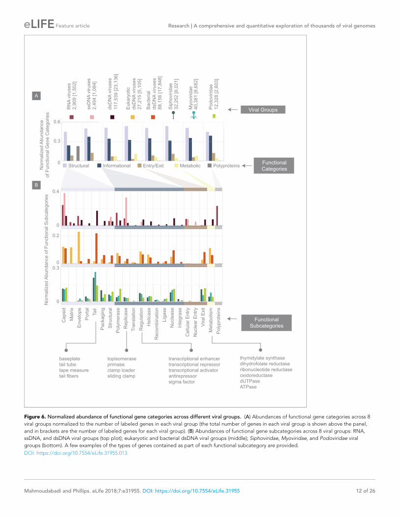
Figure 6. Normalized abundance of functional gene categories across different viral groups. (A) Abundances of functional gene categories across 8

viral groups normalized to the number of labeled genes in each viral group (the total number of genes in each viral group is shown above the panel,

and in brackets are the number of labeled genes for each viral group). (B) Abundances of functional gene subcategories across 8 viral groups: RNA,

ssDNA, and dsDNA viral groups (top plot); eukaryotic and bacterial dsDNA viral groups (middle); Siphoviridae, Myoviridae, and Podoviridae viral

groups (bottom). A few examples of the types of genes contained as part of each functional subcategory are provided.






Figure 7. Alignment of the most common gene order patterns for dsDNA bacterial viruses. Each genome is

summarized by a sequence of letters, with each letter corresponding to a gene, positioned in the order that it

appears on the genome. As an example, the gene order sequence for Salmonella phage FSL SP-004 is shown.

Note the letters shown serve to only denote genes with similar functions. Structural genes are assigned colors,

whereas other genes are denoted in black. Across all three panels, each row corresponds to the gene order

sequence for a given virus, and thus, the length of the sequence denotes the number of genes within a given

genome. The left two columns accompanying each panel provide further information on hosts and viral

morphologies. Panel A, B, and C, represent gene order patterns A, B, and C, respectively. Geneious global

alignment (Steitz et al., 2011) was used to align gene order sequences (see Materials and methods). Refer to





(Mattick and Makunin, 2006; Morris, 2012).

With a median noncoding percentage of just

6%, RNA viral genomes have significantly lower

noncoding percentage compared to DNA

viruses in this database (one-sided Mann-Whit-

ney U Test, P<10-5). A notable exception to the

RNA viral group is the ssRNA-RT with a median

noncoding percentage of 16%. Interestingly,

both retroviral groups had relatively high non-

coding DNA percentages. This is likely due to

the presence of defunct retroviral genes. For

example, the Xenopus laevis endogenous retro-

virus (NCBI taxon ID 204873) belonging to the

ssRNA-RT group has a noncoding percentage of

93%. This high noncoding percentage can be

explained by the fact that this virus genome con-

tains three pseudogenes previously coding for

env, pol and gag proteins.

Viral functional gene categories

We categorized viral genes according to several

major functional categories, including structural

genes such as capsid and tail genes, metabolic

genes, informational genes, which we define as

those involved in replication, transcription or

translation of the viral genetic code, among

other categories (Figure 6, see Materials and

methods). In addition to the fraction of viral

genes that we were able to assign to these func-

tional categories, there still remains what we will

refer to as an “unlabeled” fraction that is com-

prised of hypothetical genes or genes with poor

annotation (see Materials and methods). When

reporting the relative abundance of different

functional gene categories, we will normalize the

number of genes belonging to each functional

category by the total number of labeled genes.

RNA, dsDNA and ssDNA viruses, despite dif-

ferences in the detailed categorization of their

genes (Figure 6B) share similar general features

(Figure 6A). For example, across all three viral

groups, roughly half of all genes are structural.

Similarly, dsDNA viruses of eukaryotes and bac-

teria in this database, in contrast to having dif-

ferent genomic properties and morphologies

surprisingly have very similar distribution of gene

functional category and subcategory abundan-

ces. The major difference between these two

viral groups, as expected from our knowledge of

viral morphologies, is that a larger portion of

eukaryotic dsDNA viral genes are envelope and

matrix genes, whereas a greater portion of bac-

terial dsDNA genes are portal and tail-associ-

ated genes. By further zooming in on bacterial

dsDNA viruses, it is again interesting to see that

Myoviridae, Siphoviridae, and Podoviridae viral

groups, with their different morphologies and

wide range of hosts, having very similar func-

tional gene category abundances even at the

level of subcategories.

Viral genome organization

To explore viral genome organization we devel-

oped a coarse-grained method for visualizing a

large number of genomes in one snapshot. We

first defined genome organization as the order

in which genes appear across a genome. We

then symbolized each gene by a letter, indiffer-

ent to the gene’s length or its orientation on the

genome. Genes with similar functions are

grouped and are represented by the same letter

(Figure 7). Therefore each viral genome, analo-

gous to a nucleotide sequence, is compactly

described by a sequence of letters that repre-

sent its gene order (Figure 7), which we will

refer to as the gene order sequence. Because

we aimed to study gene order sequences across

different viral groups, we focused on genes

whose functions are universally required, namely

structural genes. textFile-1.txt (see our GitHub

repository) provides the structural gene order

sequences for all viruses (see Materials and

methods for filters applied), though the script

developed can be modified to visualize the

placement of any number of genes or user-

defined gene groups.

Furthermore, by focusing on bacterial dsDNA

viruses present in the NCBI viral database, we

were able to identify the most common gene

order patterns across this virome (see Materials

Figure 7 continued

Figure 7—figure supplement 1 to see the percent identity heat maps of terminases (large and small subunits)

across dsDNA bacterial viruses.



Figure supplement 1. Percent identity heat maps of A) 320 terminase (large subunit) amino acid sequences, and

B) 191 terminase (small subunit) amino acid sequences from dsDNA bacteriophages.







and methods). One particular gene order pat-

tern and its variations exist across various types

of dsDNA bacterial viruses. We will refer to it as

gene order pattern A (Figure 7A). In pattern A,

gene packaging, portal and capsid-related

genes are mostly tightly clustered and are fol-

lowed by tail-associated genes. Interestingly,

this pattern occurs at the beginning of the

genome for some viruses, and for others it

seems to have been shifted further down on the

genome. Pattern A occurs across viruses from

five different host phyla. The other two most

common gene order patterns (patterns B and C)

occur across viruses with more limited host

range and morphologies.

Beyond their order in the genome, we won-

dered to what extent are bacteriophage pro-

teins from taxonomically similar hosts similar to

each other in sequence? In an attempt to

address this question, we analyzed sequences

from two structural proteins in dsDNA bacterio-

phages, namely terminase large subunit and

small subunit, which are used in the packaging

of DNA inside capsids and represent some of

the more clearly annotated bacteriophage pro-

teins. Amino acid sequences were aligned using

Clustal-Omega (Arndt et al., 2016) and the

Figure 8. Attachment site length, position, and sequence diversity for 164 dsDNA bacterial viruses. (A) Histogram of attachment site length. (B)

Histogram of attachment site start positions (left attachment: blue, right attachment: red). (C) Histogram of attachment site start positions normalized

by the genome length. (D) Percent sequence similarity matrix across attachment sites. (E) Attachment site locations along viral genomes (left

attachment: blue, right attachment: red). Figure 8—source data 1 demonstrates several bacteriophages shown in panel E with similar or identical

attachment site sequences.



Source data 1. Several bacteriophages from Figure 8D with similar or identical attachment site sequences.







sequence similarity percentages are shown as

heat maps (Figure 7—figure supplement 1).

The host phylum information is color-code. As

can be seen from this figure, bacteriophages

infecting hosts from the same phylum do not

necessarily have more similar terminase sequen-

ces. In the cases where there is a similarity

between terminase sequences, it is primarily

from bacteriophages infecting the same host

species.

To provide more information on the genomic

organization of dsDNA bacteriophages, we

examined attachment site positions, length dis-

tributions, and sequence diversity. Attachment

sites are locations of site-specific recombination

that lysogenic phages use to insert their DNA

into the host genome (See Materials and meth-

ods). Among the several hundred dsDNA bac-

teriophages that were included in this analysis,

we found roughly a quarter to have putative

attachment sites. We found that the median

attachment site length is 13 base pairs

(Figure 8A). The left attachment start position in

the genome is located at ~2 kb (this is the

median of left attachment site start positions

across all genomes analyzed). The right attach-

ment site median position is located at ~40 kb.

(Figure 8B). Figure 8C demonstrates the same

data but normalized by the genome length.

To examine attachment site sequence diver-

sity, we used Clustal-Omega (Sievers et al.,

2011) for creating a sequence alignment.

Figure 8D is a heat map of the percent

sequence similarity scores. Figure 8E demon-

strates left (blue) and right (red) attachment sites

in phage genomes. Note, the genomes are

shown according to their order in Figure 8D.

While the vast majority of attachment sites are

very diverse in sequence, as shown by regions of

low similarity in the heat map, there are a num-

ber of viruses that have identical putative attach-

ment site sequences (Figure 8—source data 1,

Materials and methods). Perhaps not surpris-

ingly, these phages are largely those infecting

different strains of the same host species.

Phages infecting hosts outside of the same spe-

cies seem more likely to have dissimilar attach-

ment site sequences.

Shedding some light on viral“hypothetical” proteins

As demonstrated in the previous sections, pro-

teins annotated as hypothetical or putative form

more than half of all proteins associated with

dsDNA bacteriophages. In an attempt to learn

more about these proteins, we used BLASTP to

query all ~88,000 dsDNA bacteriophage pro-

teins against the NCBI Refseq protein database

(limited to bacteria) (See Materials and

4,000 17,000 16,000 14,000

dsDNA bacteriophage

proteins

51,000 37,000

30,0007,00021,000 30,000

Un-annotated Annotated

With bacterial

homolog

With bacterial

homolog

No bacterial

homolog

No bacterial

homolog

Annotated bacterial

homolog

Un-annotated bacterial

homolog

Annotated bacterial

homolog

Un-annotated bacterial

homolog

BLASTP results (phage proteins vs. bacterial proteins)

88,000

Figure 9. The result of BLASTP for all dsDNA bacteriophage proteins against the NCBI Refseq protein database

(limited to bacterial proteins). The numbers reported correspond to the number of dsDNA bacteriophage

proteins (rounded to the nearest thousand).






methods). The purpose of this exercise was to

use the annotations of bacterial homologs to

viral proteins to gain better understanding of

what the function of each bacteriophage hypo-

thetical protein might be.

A homologous relationship was defined as a

match with BLASTP E-value score < 10-10. The

closest bacterial homolog to each bacterio-

phage protein (i.e. the match with the lowest

E-value) was collected. Not all bacteriophage

proteins had a bacterial homolog, at least not

one that is currently in the NCBI database. How-

ever, a surprisingly large number did have bacte-

rial homologs, and we have collected these

proteins along with other useful information in

textFile-2.txt (see our GitHub repository). This

dataset is in part visualized in Figure 9.

Most bacterial homologs of hypothetical

phage proteins were also annotated as hypo-

thetical proteins. However, a few thousand

hypothetical phage proteins could be assigned

to putative annotation based on the annotation

of their bacterial homologs (See Materials and

methods). Interestingly, we were able to match

even more bacterial hypothetical proteins to a

putative annotation based on the annotations of

their bacteriophage protein homologs.

Although, this method can certainly be helpful in

filling some of the gaps in protein annotations, it

is only as good as the annotations and the con-

vention we establish for describing proteins.

Unfortunately, a considerable number of annota-

tions are currently either too specialized or too

vague to be helpful.

The extent of overlap between viral andcellular gene pools

One of the defining features of viruses is their

reliance on their host organisms. It is well known

that the interactions between viruses and cells

often result in the exchange of genetic informa-

tion. To explore the extent to which the viral

and cellular gene pools overlap, we used

BLASTP to search for bacterial proteins that are

homologous to dsDNA bacteriophage proteins

(see Materials and methods). Overall, each of

the ~900 dsDNA bacteriophage genomes we

examined encoded at least one protein that was

homologous to a bacterial protein.

To systematically examine the extent of

homology between bacteriophage and bacterial

proteins, we calculated the number of proteins

per bacteriophage genome with homology to a

bacterial protein, and divided this number by

the total number of proteins encoded by the

bacteriophage genome. In Figure 10—figure

supplement 1 (left), we demonstrate the histo-

gram of the fraction of homologous proteins per

bacteriophage genome. Based on the median

fraction of homologous proteins, we can con-

clude that 7 out of every 10 bacteriophage pro-

teins exhibit homology to a bacterial protein.

This suggests that there is a significant overlap

between the two gene pools.

There are multiple mechanisms by which a

bacterial protein and a bacteriophage protein

could exhibit homology. The most trivial, con-

ceptually, is when the same protein is registered

as part of both a bacterial genome and a bacte-

riophage genome, as it would be for a prophage

protein. In the case of prophages, we would

expect to see a high fraction of bacteriophage

proteins per genome that are homologous to

bacterial proteins since their genomes should at

some point in time be embedded in their hosts’

genomes.

Thus, to examine the contribution from pro-

phages, we implemented several filters to iden-

tify probable prophage genomes (see Materials

and methods). Based on these filters, 173

genomes were identified. These genomes were

primarily contributing to the large spike in the

left histogram in Figure 10—figure supplement

1. To evaluate these filters, we performed a liter-

ature search for the first 20 bacteriophage

genomes in the list and found that the majority

were, in fact, experimentally identified as tem-

perate phages. Because we could not find a

database that contained a list of all experimen-

tally verified prophages and their lytic relatives

to compare our predictions to, we did not

exclude these genomes from further analysis.

A non-trivial mechanism by which bacterio-

phages and bacteria can exhibit homologous

proteins is via gene exchanges over evolutionary

time-scales. Interestingly, the closest homolog

to a bacteriophage protein is not always found

in its host genome. In fact there can be large

taxonomic distance (Figure 10) between the

host and the bacterium containing the closest

homolog. We depict this distance by categoriz-

ing bacteriophage proteins based on the organ-

ism in which their closest homolog was found

(see inscribed circles in Figure 10). If they were

found in the same species of bacteria as the

host, then these proteins are placed in the most

inner circle, whereas if they were found in the

same phylum, the proteins are placed in the

outer most circle.

We can see from Figure 10 that there is a

26% chance that the closest homolog to a bacte-

riophage protein appears in a member of its




host species. This chance is raised to 84% when

more broadly assuming that the homolog will

appear in a bacterium that is at least in the same

phylum as the host (Figure 10). The chance

value is calculated by dividing the number of

proteins in a given taxonomic layer by the total

number of proteins in the analysis.

Moreover, an interesting facet of this dataset

becomes apparent when we examine the quality

of the match between a bacteriophage protein

and its closest bacterial homolog as a function

of the taxonomic distance between the bacterio-

phage host and the bacterium containing the

homolog. We used the bit score as a measure of

quality of the match. The bit score is a BLAST

output and a similarity measure that is indepen-

dent of database size or the query sequence

length. It identifies the size of a database

required for finding the same quality match by

chance. Naturally, the higher the bit score, the

better is the match.

We can see that there is a significant

decrease in the median bit score as we move

from the “same species” layer to the “same

genus” layer and finally to the “same

phylum” layer (Figure 11). Thus, the closer (tax-

onomically) the host is to the bacterium contain-

ing the homolog, the better the match between

the bacteriophage protein and its bacterial

homolog. We think there are interesting phage-

host co-evolutionary implications that can be

concluded from this data analysis and data visu-

alization method, and hope to shed further light

on these hypotheses in the future.

While the majority of homologs belong to

members of the same phylum as the host, there

is still a 16% chance that the closest bacterial

homolog to a bacteriophage protein actually

Figure 10. A depiction of the taxonomic distance between the bacteriophage host organism and the bacterium

containing the closest homolog to a bacteriophage protein. All circles are drawn to scale with respect to the

number of proteins (N) that they each represent. Note, the number of proteins denoted at each taxonomic layer

includes proteins in lower taxonomic layers. For example, the 20,000 figure denoted at the genus layer already

includes the 11,000 proteins shown at the species layer. N values are rounded to the nearest thousand.

Histograms of the fraction of proteins with bacterial homologs per bacteriophage genome are shown in




Figure supplement 1. Histogram of the fraction of proteins per bacteriophage genome with bacterial homologs

(Left) and the same histogram with an additional filter to identify possible prophages and their lytic relatives

(right).







appears in a bacterium from a different phylum

than the host. To further examine these cross-

phyla associations, we map the distribution of

bacteriophage proteins as a function of the host

phylum. Then, we zoom in on the bacterial phyla

containing the homologs (Figure 11—figure

supplement 1). By far, the most number of

cross-phyla homologs are shared between bac-

teriophages infecting Proteobacteria and bacte-

ria from the Firmicutes phylum. It would be

interesting to explore in the future the underly-

ing cause of the relatively large number of

homologs that exist between microbial members

of the Firmicutes and Proteobacteria phyla.

DiscussionOur primary motivation for conducting a large-

scale study of viral genomes was to provide the

distributions of key numbers that characterize

viral genomes. However, it is important to note

that while the NCBI viral database represents a

large collection of complete viral genomes, it

still represents a small fraction of the total viral

diversity in nature. In light of the striking geno-

mic trends observed across different viral

groups, future studies are needed to re-examine

these trends as our databases grow in size with

greater focus on several underrepresented

groups such as archaeal viruses and bacterial

RNA viruses. To that point, upon re-examining

Same genus

Same species

Same phylum

Same species

Same species

median = 285

Same genus

median = 201

1000 200000

2000

4000

1000 200000

2000

4000

Nu

mb

er

of

pro

tein

sN

um

be

r o

f p

rote

ins

Same species

median = 285

Same phylum

median = 156

p < 0.001

p < 0.001

Bit score

Bit score

A

B

Figure 11. Histograms of bit scores describing the match between each bacteriophage protein and its closest

bacterial homolog. Histograms are created according to the proteins belonging to three different layers

corresponding to an increasing taxonomic distance between the host organism and the bacterium containing the

closest homolog. (A) When the host and the homolog-containing bacterium belong to the same species, the

median bit score is significantly higher (one sided Mann-Whitney U test, P<0.001) than it is for those that are only

part of the same genus. (B) Similarly, when comparing proteins from the “same species” layer to the “same

phylum” layer, the median bit score is significantly higher for the “same species” layer (one sided Mann-Whitney

U test, P<0.001). Note that for each layer, when comparing the “same species” to the “same genus” layers, we are

comparing the 11,000 proteins in the “same species” layer to the 9,000 proteins from the “same genus” layer that

do not also belong to the “same species” layer. The same principle applies when we are comparing the “same

species” layer to the “same phylum” layer. Distributions of bacteriophage proteins with homologs from a different

phylum than their host phylum are shown in Figure 11—figure supplement 1.



Figure supplement 1. Distributions of bacteriophage proteins with a homolog in a bacterium from a different

phylum than their host phylum.







the NCBI viral database in 2018, we were sur-

prised to find that eventhough the database has

almost doubled in size, the increase has dispro-

portionately favored the already well-repre-

sented viral groups. Thus, the underrepresented

groups continue to be underrepresented.

Our second motivation for conducting this

study was to compare different viral classifica-

tion systems. Because viral classification systems

were constructed prior to the emergence of

sequencing, we were interested to see how well

they can describe genomic trends. Based on a

comparison of classification systems across vari-

ous genomic metrics, the Baltimore classification

and in some cases its more minimal form (Nucle-

otide Type classification) seem to provide the

clearest explanation for the observed trends.

We suspect that this is due to the Baltimore clas-

sification’s discernment of RNA, ssDNA and

dsDNA genomes, which have striking physical

differences.

The greater stability of dsDNA compared to

RNA (Lindahl, 1993) and ssDNA is thought to

be an important factor in the observed variations

in genome lengths. The 2’-hydroxyl group in

RNA makes it more susceptible to hydrolysis

events and cleavage of the backbone compared

to DNA. It has been shown that for bacteria and

viruses, the mutation rate and the genome

length are inversely correlated (Drake, 1991;

Sanjuan et al., 2010), and it is therefore hypoth-

esized that the lack of proofreading mechanisms

in RNA replication and the resulting higher

mutation rates compared to DNA replication

(Sanjuan et al., 2010) imposes length limits on

RNA viral genomes. In support of the suspected

link between mutation rates and genome length,

it has been shown that long RNA viruses (above

20 kb) contain 3’-5’ exonuclease, which is a

homolog of the DNA-proofreading enzymes

(Lauber et al., 2013).

Similarly, the hydrolysis of cytosine into uracil

occurs two orders of magnitude faster in ssDNA

genomes than in dsDNA genomes

(Frederico et al., 1990). This may explain the

high mutation rates of ssDNA viruses, which is

within the range of RNA viral mutation rates,

despite using error-correcting host polymerases

to replicate. In contrast to genome length in

which ssDNA and RNA viruses have similar distri-

butions, it was interesting to see that ssDNA

viruses are actually more similar to dsDNA

viruses in terms of their gene lengths and non-

coding percentages.

While the Baltimore classification serves as a

meaningful coarse-grained classification system,

it is historically animal virus centric and will bene-

fit from being expanded to include subcatego-

ries discerning of bacterial and archaeal viruses.

As shown by gene length distributions (Figure 4),

the additional layer of categorization provided

by the Host Domain classification offers new

insight. For example, dsDNA and ssDNA viruses

of eukaryotes have much longer gene lengths

compared to their prokaryotic counterparts- an

observation that may be hinting at the coevolu-

tion of host and viral genomes and proteomes

since the eukaryotic genes and proteins are also

shown to be significantly longer than prokaryotic

ones (Brocchieri and Karlin, 2005; Zhang, 2000;

Tiessen et al., 2012). It is well known that cer-

tain eukaryotic viral genomes, similar to their

hosts’ genomes, contain genes with introns

(Himmelspach et al., 1995; Barksdale and

Baker, 1995; Ge and Manley, 1990), which may

explain the longer median gene length for

eukaryotic viruses. In fact mRNA splicing was

discovered for the first time in a study of adeno-

virus mRNA expression (Flint et al., 2000). Virus

proteomes are also shown to be tuned to their

hosts’ proteomes by having similar codon usage

and amino acid preferences (Bahir et al., 2009).

However, future studies are needed to further

ascertain the mechanisms responsible for the dif-

ferences in eukaryotic and prokaryotic viral gene

lengths.

The ICTV classification, which is used perhaps

more than any other classification system to

describe bacterial and archaeal viruses offers

some supporting data (e.g. viral morphology or

in some cases host information), perhaps as the

final layer of classification. However, it is limited

by the fact that it leaves many viruses unclassi-

fied and, more importantly, that it lacks truly sys-

tematic classification criteria. As our exploration

of viruses shifts its basis from culturing of viruses

to sequencing of viruses from their natural habi-

tats, morphological data is likely to become

more and more scarce. As a result, ICTV will

need to adapt its classification system to oper-

ate exclusively on genomic data, a viewpoint

that is broadly shared by many experts in the

field (Simmonds et al., 2017).

In this work, we have described our attempt

at providing a comprehensive and quantitative

view of fully sequenced viral genomes. Similar to

earlier work on biological numeracy, as exempli-

fied by the BioNumbers database (Milo et al.,

2010), we have identified a number of interest-

ing trends associated with viral genomes that

will be helpful in gaining a broad overview of




vastly different viral groups and their interactions

with their hosts.

Materials and methods

Data acquisition, data curation, andstatistical analysis

All genomic data was retrieved from the NCBI

Genome FTP server (retrieved in August 2015)

(Brister et al., 2015). Matching viruses to their

hosts was done by parsing ASN files from the

NCBI Genome FTP server while searching for

the term “nat-host”. All other taxonomic data,

including host and viral lineages, was retrieved

from NCBI’s Taxonomy database using the NCBI

Taxa class of the ETE Toolkit (Huerta-

Cepas et al., 2010). Once we had the “nat-

host” name of organisms in English, we

retrieved their taxids using ETE Toolkit. These

were in turn used to identify the host’s taxo-

nomic lineage. Viruses with complete genomes

were identified by searching the assembly

reports of the NCBI Genome FTP server for

assemblies labeled “Complete Genome”, then

using the associated FTP address to download

the _assembly_stats.txt files and _protein.faa

files. Only viruses that could be matched to a

host were included for further analysis. Addition-

ally, various quality checks were manually per-

formed to ensure that viruses with improper

annotations were excluded from further analysis.

For example, we found viruses and hosts with

incomplete or incorrect taxonomic information,

and excluded these viruses from further analysis.

The list of excluded viruses can be found in our

code (see next sub-section). Outliers are not

excluded from our analysis. We attempt to

dampen their effect by focusing on median val-

ues rather than the mean (Table 1). Given the

presence of a few skewed distributions, we pri-

marily used the Mann-Whitney U test for statisti-

cal analysis so we could avoid the assumption of

normality.

Data availabilityWe have compiled all input data, output files, andscripts (Jupyter notebooks) used to write this manu-script in a GitHub repository (https://github.com/gita-mahm/VirologyByTheNumbers) (Mahmoudabadi,2018). viromePieChartsVF.ipynb and virusHostHistog-ramsVF.ipynb were used to create Figure 2. The scriptsfor Figure 3 through Figure 5 can be found ingenomeLengthsVF.ipynb, geneLengthsVF.ipynb, andpercentNoncodingVF.ipynb, respectively. The code forFigure 6 and Figure 7 is provided in geneOrderAndG-eneAbundanceVF.ipynb. viralAttachmentSites.ipynb isused to create Figure 8 and viralBacterialBlast.ipynb is

used to create (Figures 9–11 and their supplementaryfigures).

All supplementary text files can also be found in thisrepository. Supplementary textFile-1.txt displays thegene order sequences for all viruses whose genomescontained at least 15% labeled genes. Letters I, C, E,and Q correspond to capsid-related, portal-related,tail-related, and genome packaging-related genes,respectively. All other genes are denoted by the letterA. Supplementary textFile-2.txt contains the list of topBLASTP matches for bacteriophage proteins that hadbacterial protein homologs (the top match isconsidered as the match with the lowest E-value). Sup-plementary textFile-3.txt provides the annotations ofbacterial homologs of hypothetical bacteriophage pro-teins. Supplementary textFile-4.txt contains the annota-tions of bacteriophage homologs of hypotheticalbacterial proteins.

Genome length and gene densities

Genome lengths were extracted from .ptt files

and _assembly_stats.txt files for viruses. The .ptt

files were parsed to find “complete genome -

1.” which is followed by the length of the

genome. For segmented genomes, the total

length of the segments is reported as the

genome length. The number of protein-coding

genes, which was used in calculating gene densi-

ties, was found by parsing .faa files . For gene

length histograms, we first obtained the gene

lengths for each virus, and then created a histo-

gram based on the median gene length associ-

ated with each virus. To

systematically determine the number of bins

needed for each histogram, we employed the

Freedman-Diaconis’ rule (Freedman and Diaco-

nis, 1981).

Noncoding DNA/RNA percentages

To extract the percent of the genome that is

noncoding, we could not merely subtract the

lengths of the genes from the length of the

genome, as this would not take overlapping

genes into account. Instead, we used the .ptt

files to identify where each gene began and

ended in the genome, then added all indices

between protein-coding genes to a set. We then

could subtract the size of this set from the

genome length to arrive at the number of non-

coding bases, which is then turned into a

percentage.

Decomposition of viral genes intofunctional categories

To obtain the abundance of various gene func-

tional categories, we collected the COG product

annotations (Tatusov et al., 2000) accompa-

nying each gene from .ptt file(s) provided for



https://github.com/gitamahm/VirologyByTheNumbers



each virus. Based on the most frequent COG

product names, we constructed a dictionary of

search terms to query viral genes and measure

the abundance of various functional categories

(by measuring abundance, we are referring to

the number of genes that belong to a given

functional category). To determine the most

common search terms, we derived the unique

set of COG product annotations for different

viromes. We used the annotations shared

between viromes to exclude problematic search

terms with multiple meanings. As a result we

avoided search terms with multiple functional

associations such as “gp41”, which in the con-

text of HIV signifies a transmembrane glycopro-

tein, and in the context of Mycobacterium

phage Bxb1 denotes a 3’-5’ exonuclease

involved in DNA replication.

While the dictionary constructed contains

many key words that capture essential gene

functional categories common to many viruses,

it does not account for COG annotations that

are non-descriptive (e.g. “phage protein” or “Z

protein”). Additionally, there is typically a large

number of genes that code for “hypothetical

proteins”. Together, these two fractions make

up the unlabeled component, which we do not

include for further analysis. Despite the limita-

tions introduced by these unlabeled genes,

there are still a large number of genes (~105)

that are included in our analysis. In constructing

the relative abundances of different gene func-

tional categories (Figure 6), we divide the abun-

dance of a gene functional category by the total

number of labeled genes (denoted at the top of

Figure 6.A for each viral group).

Gene order

In visualizing gene order we employed a similar

search strategy to the one explained in the pre-

vious section. To detect potentially conserved

patterns in gene order across vastly different

viral genomes, we searched only for structural

genes as they are essential to any virus. We

used .ptt files to determine gene order since

they contain the beginning and end indices of

genes. The code developed uses .ptt files as

input, and outputs a string of characters per viral

genome, which we have referred to as the gene

order sequence. Each character represents a

viral gene in the order that it appears on the

genome (without distinguishing between the

strand of DNA on which the gene is located). All

genes belonging to the same functional cate-

gory, for example all tail-related genes, are rep-

resented by the same character. All unlabeled

genes (i.e. non-structural, hypothetical, or poorly

annotated genes) are also represented by the

same character. Each gene order sequence,

analogous to a nucleotide sequence, can be

aligned against other gene order sequences by

existing alignment software.

Though it would be ideal to calculate a pair-

wise distance matrix between gene order

sequences and to quantitatively define a gene

order pattern based on gene order sequence

similarity (akin to defining an Operational Taxo-

nomic Unit), this effort would require the devel-

opment of appropriate alignment algorithms

and inference methods fit to process gene order

sequences. In the meantime, we used existing

alignment software as a guide and grouped

gene order sequences based on generally

shared features.

We used Geneious software (Kearse et al.,

2012) to align gene order sequences using

global alignment with free end gaps and identity

cost matrix (with default gap open and exten-

sion penalties). Using Geneious global alignment

as a guide, we further manually improved the

alignment by aligning a widely shared sub-pat-

tern, for example the portal/neck genes in pat-

tern A or the capsid and tail characters in

pattern C, without introducing any gaps. This

step was necessary because any alignment algo-

rithm will aim to maximize the alignment

between unlabeled genes, unable to distinguish

between these characters and the more mean-

ingful characters corresponding to labeled struc-

tural genes. Moreover, because of the high

fraction of genes that have “hypothetical pro-

tein” COG annotation, we had to impose filters

to extract gene order sequences that are not

entirely composed of unlabeled genes. To gen-

erate the alignments shown in Figure 7, we

imposed that at least 15% of characters in a

gene order sequence have to correspond to

labeled genes, and that the gene order

sequence has to be at least 40 characters long.

For the gene order sequences shown in textFile-

1.txt (see GitHub repository) the sequence order

length limit was not imposed.

Bacteriophage attachment sites

To explore bacteriophage attachment sites, we

used the PHASTER program to obtain putative

attachment sites (Arndt et al., 2016). Using

phage genome accession numbers and the

PHASTER URL API, we obtained information

regarding attachment site sequence and loca-

tion. We analyzed and visualized this data using

our own set of scripts, which can be found in the




attachmentSites.ipynb notebook. When compar-

ing attachment site sequences, we selected

phage pairs with 100% similarity across their

alignment. We also imposed that the alignment

length should be at least 8 bp (which is more

than half of the median attachment site length).

Figure 8—source data 1 depicts phages that

met these criteria.

BLASTing dsDNA bacteriophage proteinsagainst bacterial proteins

Multithreaded BLASTP on this database was a

computationally intensive process, requiring

over 8900 core hours. Using custom scripts in R,

taxID results from each protein queried were

linked to complete lineages using NCBI tax-

dump and NCBItax2lin (available via https://

github.com/zyxue/ncbitax2lin). A list of hypo-

thetical bacteriophage proteins and their closest

bacterial homologs are provided in textFile-3.txt

(see our GitHub repository). Similarly the hypo-

thetical bacterial proteins along with the annota-

tions of their closest bacteriophage homologs

are provided in textFile-4.txt. The closest homo-

logs are determined based on the match with

the lowest E-value. A match was taken into

account only if it had an E-value < 10-10.

Identifying putative prophage genomes

We suspected that prophage proteins would

have a high percent identity to their bacterial

homologs, and therefore, we first filtered pro-

teins with less than 50% identity to their bacterial

homologs. We then selected only proteins with

bacterial homologs if the bacterium containing

the homolog was the same species as the bacteri-

ophage host. Finally, we required that at least

half of the proteins per bacteriophage genome

meet the conditions described above for the bac-

teriophage to be identified as a potential pro-

phage. The reason we did not impose stricter

filters was so that we could also identify any lytic

relatives of prophages, since their proteins would

also be perceived homologous to bacterial pro-

teins, but only because of their homology to pro-

phage proteins.

Acknowledgements

We thank Arup Chakraborty, Markus Covert and

Richard Neher for their helpful suggestions

through the review process. We would addition-

ally like to thank Bill Gelbart, Eddy Rubin, Forest

Rohwer, Eugene Shakhnovich, Matt Morgan, and

members of the Phillips Lab and the Boundaries

of Life Initiative for helpful discussions. We would

like to especially thank Helen Foley for helping us

run BLAST using Amazon cloud computing serv-

ices. This study was supported by the National

Science Foundation (Graduate Research

Fellowship; DGE-1144469), the John Templeton

Foundation (Boundaries of Life Initiative; 51250),

the National Institute of Health (Maximizing

Investigator’s Research Award; RFA-GM-17-002),

the National Institute of Health (Exceptional

Unconventional Research Enabling Knowledge

Acceleration; R01- GM098465), and the National

Science Foundation (NSF PHY11-25915) through

the 2015 Cellular Evolution course at the Kavli

Institute for Theoretical Physics.

Gita Mahmoudabadi is in the Department of

Bioengineering, California Institute of Technology,

Pasadena, United States

http://orcid.org/0000-0002-8812-7246

Rob Phillips is in the Department of Bioengineering

and the Department of Applied Physics, California

Institute of Technology, Pasadena, United States

[email protected]

http://orcid.org/0000-0003-3082-2809

Author contributions: Gita Mahmoudabadi, Concep-

tualization, Data curation, Formal analysis, Supervision,

Validation, Visualization, Methodology, Writing—origi-

nal draft, Project administration, Writing—review and

editing; Rob Phillips, Conceptualization, Supervision,

Funding acquisition, Investigation, Methodology, Proj-

ect administration, Writing—review and editing

Competing interests: The authors declare that no

competing interests exist.

Received 17 September 2017

Accepted 30 March 2018

Published 19 April 2018

Funding

FunderGrant referencenumber Author

John TempletonFoundation

51250 Rob Phillips

National Insti-tutes of Health

RFA-GM-17-002 Rob Phillips

National ScienceFoundation

DGE-1144469 GitaMahmoudabadi

National Insti-tutes of Health

R01- GM098465 Rob Phillips

National ScienceFoundation

NSF PHY11-25915

Rob Phillips

The funders had no role in study design, data

collection and interpretation, or the decision to submit

the work for publication.



https://github.com/zyxue/ncbitax2lin

https://github.com/zyxue/ncbitax2lin

http://orcid.org/0000-0002-8812-7246

http://orcid.org/0000-0003-3082-2809


Decision letter and Author response

Decision letter https://doi.org/10.7554/eLife.31955.027

Author response https://doi.org/10.7554/eLife.31955.

028

Additional files

Supplementary files. Transparent reporting form


Major datasetsThe following dataset was generated:

Author(s) Year DatasetURL

Database,license,andaccessibilityinformation

Brister JR, Ako-Adjei D, Bao Y,Blinkova O

2015 ftp://ftp.ncbi.nlm.nih.gov/refseq/re-lease/viral/

Publiclyavailable at theNCBI viralresource page(https://www.ncbi.nlm.nih.gov/genome/viruses/)

References

Alberts B, Johnson A, Lewis J, Walter P, Raff M,Roberts K. 2002. Molecular Biology of the Cell 4thEdition: International Student Edition. Routledge.Arndt D, Grant JR, Marcu A, Sajed T, Pon A, Liang Y,Wishart DS. 2016. PHASTER: a better, faster version ofthe PHAST phage search tool. Nucleic Acids Research44:W16–W21. DOI: https://doi.org/10.1093/nar/gkw387, PMID: 27141966Bahir I, Fromer M, Prat Y, Linial M. 2009. Viraladaptation to host: a proteome-based analysis ofcodon usage and amino acid preferences. MolecularSystems Biology 5:311. DOI: https://doi.org/10.1038/msb.2009.71, PMID: 19888206Baltimore D. 1971. Expression of animal virusgenomes. Bacteriological Reviews 35:235–241.PMID: 4329869Barksdale S, Baker CC. 1995. Differentiation-specificalternative splicing of bovine papillomavirus latemRNAs. Journal of Virology 69:6553–6556.PMID: 7666558Brandes N, Linial M. 2016. Gene overlapping and sizeconstraints in the viral world. Biology Direct 11:26.DOI: https://doi.org/10.1186/s13062-016-0128-3,PMID: 27209091Brister JR, Ako-Adjei D, Bao Y, Blinkova O. 2015.NCBI viral genomes resource. Nucleic Acids Research43:D571–D577. DOI: https://doi.org/10.1093/nar/gku1207, PMID: 25428358Brocchieri L, Karlin S. 2005. Protein length ineukaryotic and prokaryotic proteomes. Nucleic AcidsResearch 33:3390–3400. DOI: https://doi.org/10.1093/nar/gki615, PMID: 15951512

Brussow H, Hendrix RW. 2002. Phage genomics: smallis beautiful. Cell 108:13–16. DOI: https://doi.org/10.1016/S0092-8674(01)00637-7, PMID: 11792317Casjens SR, Gilcrease EB, Winn-Stapley DA,Schicklmaier P, Schmieger H, Pedulla ML, Ford ME,Houtz JM, Hatfull GF, Hendrix RW. 2005. Thegeneralized transducing Salmonella bacteriophageES18: complete genome sequence and DNApackaging strategy. Journal of Bacteriology 187:1091–1104. DOI: https://doi.org/10.1128/JB.187.3.1091-1104.2005, PMID: 15659686Drake JW. 1991. A constant rate of spontaneousmutation in DNA-based microbes. PNAS 88:7160–7164. DOI: https://doi.org/10.1073/pnas.88.16.7160,PMID: 1831267Dutilh BE, Cassman N, McNair K, Sanchez SE, SilvaGG, Boling L, Barr JJ, Speth DR, Seguritan V, Aziz RK,Felts B, Dinsdale EA, Mokili JL, Edwards RA. 2014. Ahighly abundant bacteriophage discovered in theunknown sequences of human faecal metagenomes.Nature Communications 5:4498. DOI: https://doi.org/10.1038/ncomms5498, PMID: 25058116Edwards RA, Rohwer F. 2005. Viral metagenomics.Nature Reviews Microbiology 3:504–510. DOI: https://doi.org/10.1038/nrmicro1163, PMID: 15886693Elgar G, Vavouri T. 2008. Tuning in to the signals:noncoding sequence conservation in vertebrategenomes. Trends in Genetics 24:344–352.DOI: https://doi.org/10.1016/j.tig.2008.04.005,PMID: 18514361Firth AE, Brierley I. 2012. Non-canonical translation inRNA viruses. Journal of General Virology 93:1385–1409. DOI: https://doi.org/10.1099/vir.0.042499-0,PMID: 22535777Flint SJ, Enquist LW, Racaniello VR, Skalka AM. 2000.Principles of Virology: Molecular Biology,Pathogenesis, and Control of Animal Viruses.Washington, DC: ASM Press.Forterre P. 2010. Defining life: the virus viewpoint.Origins of Life and Evolution of Biospheres 40:151–160. DOI: https://doi.org/10.1007/s11084-010-9194-1,PMID: 20198436Frederico LA, Kunkel TA, Shaw BR. 1990. A sensitivegenetic assay for the detection of cytosinedeamination: determination of rate constants and theactivation energy. Biochemistry 29:2532–2537.DOI: https://doi.org/10.1021/bi00462a015, PMID: 2185829Freedman D, Diaconis P. 1981. On the histogram as adensity estimator: L2 theory. Zeitschrift furWahrscheinlichkeitstheorie und Verwandte Gebiete 57:453–476. DOI: https://doi.org/10.1007/BF01025868Ge H, Manley JL. 1990. A protein factor, ASF, controlscell-specific alternative splicing of SV40 early pre-mRNA in vitro. Cell 62:25–34. DOI: https://doi.org/10.1016/0092-8674(90)90236-8, PMID: 2163768Grilli J, Bassetti B, Maslov S, Cosentino LagomarsinoM. 2012. Joint scaling laws in functional andevolutionary categories in prokaryotic genomes.Nucleic Acids Research 40:530–540. DOI: https://doi.org/10.1093/nar/gkr711, PMID: 21937509Hendrix RW. 2003. Bacteriophage genomics. CurrentOpinion in Microbiology 6:506–511. DOI: https://doi.org/10.1016/j.mib.2003.09.004, PMID: 14572544Himmelspach M, Cavaloc Y, Chebli K, Stevenin J,Gattoni R. 1995. Titration of serine/arginine (SR)splicing factors during adenoviral infection modulates







ftp://ftp.ncbi.nlm.nih.gov/refseq/release/viral/




https://www.ncbi.nlm.nih.gov/genome/viruses/




https://doi.org/10.1093/nar/gkw387

https://doi.org/10.1093/nar/gkw387

http://www.ncbi.nlm.nih.gov/pubmed/27141966

https://doi.org/10.1038/msb.2009.71





https://doi.org/10.1186/s13062-016-0128-3


https://doi.org/10.1093/nar/gku1207

https://doi.org/10.1093/nar/gku1207


https://doi.org/10.1093/nar/gki615

https://doi.org/10.1093/nar/gki615


https://doi.org/10.1016/S0092-8674(01)00637-7

https://doi.org/10.1016/S0092-8674(01)00637-7


https://doi.org/10.1128/JB.187.3.1091-1104.2005

https://doi.org/10.1128/JB.187.3.1091-1104.2005


https://doi.org/10.1073/pnas.88.16.7160


https://doi.org/10.1038/ncomms5498

https://doi.org/10.1038/ncomms5498


https://doi.org/10.1038/nrmicro1163

https://doi.org/10.1038/nrmicro1163


https://doi.org/10.1016/j.tig.2008.04.005


https://doi.org/10.1099/vir.0.042499-0


https://doi.org/10.1007/s11084-010-9194-1


https://doi.org/10.1021/bi00462a015



https://doi.org/10.1007/BF01025868

https://doi.org/10.1016/0092-8674(90)90236-8

https://doi.org/10.1016/0092-8674(90)90236-8


https://doi.org/10.1093/nar/gkr711

https://doi.org/10.1093/nar/gkr711


https://doi.org/10.1016/j.mib.2003.09.004

https://doi.org/10.1016/j.mib.2003.09.004



E1A pre-mRNA alternative splicing. RNA 1:794–806.PMID: 7493325Hou C, Li L, Qin ZS, Corces VG. 2012. Gene density,transcription, and insulators contribute to the partitionof the Drosophila genome into physical domains.Molecular Cell 48:471–484. DOI: https://doi.org/10.1016/j.molcel.2012.08.031, PMID: 23041285Howe JA, Wang H, Fischmann TO, Balibar CJ, Xiao L,Galgoci AM, Malinverni JC, Mayhood T, Villafania A,Nahvi A, Murgolo N, Barbieri CM, Mann PA, Carr D,Xia E, Zuck P, Riley D, Painter RE, Walker SS,Sherborne B, et al. 2015. Selective small-moleculeinhibition of an RNA structural element. Nature 526:672–677. DOI: https://doi.org/10.1038/nature15542,PMID: 26416753Huerta-Cepas J, Dopazo J, Gabaldon T. 2010. ETE: apython environment for tree exploration. BMCBioinformatics 11:24. DOI: https://doi.org/10.1186/1471-2105-11-24, PMID: 20070885Hug LA, Baker BJ, Anantharaman K, Brown CT, ProbstAJ, Castelle CJ, Butterfield CN, Hernsdorf AW, AmanoY, Ise K, Suzuki Y, Dudek N, Relman DA, Finstad KM,Amundson R, Thomas BC, Banfield JF. 2016. A newview of the tree of life. Nature Microbiology 1:16048.DOI: https://doi.org/10.1038/nmicrobiol.2016.48,PMID: 27572647Hulo C, de Castro E, Masson P, Bougueleret L, BairochA, Xenarios I, Le Mercier P. 2011. ViralZone: aknowledge resource to understand virus diversity.Nucleic Acids Research 39:D576–D582. DOI: https://doi.org/10.1093/nar/gkq901, PMID: 20947564Jaillon O, Aury JM, Brunet F, Petit JL, Stange-Thomann N, Mauceli E, Bouneau L, Fischer C, Ozouf-Costaz C, Bernot A, Nicaud S, Jaffe D, Fisher S,Lutfalla G, Dossat C, Segurens B, Dasilva C,Salanoubat M, Levy M, Boudet N, et al. 2004. Genomeduplication in the teleost fish Tetraodon nigroviridisreveals the early vertebrate proto-karyotype. Nature431:946–957. DOI: https://doi.org/10.1038/nature03025, PMID: 15496914Kearse M, Moir R, Wilson A, Stones-Havas S, CheungM, Sturrock S, Buxton S, Cooper A, Markowitz S,Duran C, Thierer T, Ashton B, Meintjes P, DrummondA. 2012. Geneious basic: an integrated andextendable desktop software platform for theorganization and analysis of sequence data.Bioinformatics 28:1647–1649. DOI: https://doi.org/10.1093/bioinformatics/bts199, PMID: 22543367Keller B, Feuillet C. 2000. Colinearity and gene densityin grass genomes. Trends in Plant Science 5:246–251.DOI: https://doi.org/10.1016/S1360-1385(00)01629-0,PMID: 10838615King AMQ, Lefkowitz E, Adams MJ, Casrstens EB.2011. Virus Taxonomy: Ninth Report of theInternational Committee on Taxonomy of Viruses.Elsevier.Koonin EV, Dolja VV, Krupovic M. 2015. Origins andevolution of viruses of eukaryotes: the ultimatemodularity. Virology 479-480:2–25. DOI: https://doi.org/10.1016/j.virol.2015.02.039, PMID: 25771806Kristensen DM, Mushegian AR, Dolja VV, Koonin EV.2010. New dimensions of the virus world discoveredthrough metagenomics. Trends in Microbiology 18:11–19. DOI: https://doi.org/10.1016/j.tim.2009.11.003,PMID: 19942437Kristensen DM, Cai X, Mushegian A. 2011.Evolutionarily conserved orthologous families in

phages are relatively rare in their prokaryotic hosts.Journal of Bacteriology 193:1806–1814. DOI: https://doi.org/10.1128/JB.01311-10, PMID: 21317336Labonte JM, Swan BK, Poulos B, Luo H, Koren S,Hallam SJ, Sullivan MB, Woyke T, Wommack KE,Stepanauskas R. 2015. Single-cell genomics-basedanalysis of virus-host interactions in marine surfacebacterioplankton. The ISME Journal 9:2386–2399.DOI: https://doi.org/10.1038/ismej.2015.48, PMID: 25848873Lauber C, Goeman JJ, Parquet MC, Nga PT, SnijderEJ, Morita K, Gorbalenya AE. 2013. The footprint ofgenome architecture in the largest genome expansionin RNA viruses. PLoS Pathogens 9:e1003500.DOI: https://doi.org/10.1371/journal.ppat.1003500,PMID: 23874204Lindahl T. 1993. Instability and decay of the primarystructure of DNA. Nature 362:709–715. DOI: https://doi.org/10.1038/362709a0, PMID: 8469282Mahmoudabadi G. 2018. VirologyByTheNumbers.GitHub. 38. https://github.com/gitamahm/VirologyByTheNumbersMahy BWJ, Van Regenmortel MHV. 2010. DeskEncyclopedia of Human and Medical Virology.Academic Press.Marbouty M, Baudry L, Cournac A, Koszul R. 2017.Scaffolding bacterial genomes and probing host-virusinteractions in gut microbiome by proximity ligation(chromosome capture) assay. Science Advances 3:e1602105. DOI: https://doi.org/10.1126/sciadv.1602105, PMID: 28232956Marinelli LJ, Fitz-Gibbon S, Hayes C, Bowman C,Inkeles M, Loncaric A, Russell DA, Jacobs-Sera D,Cokus S, Pellegrini M, Kim J, Miller JF, Hatfull GF,Modlin RL. 2012. Propionibacterium acnesbacteriophages display limited genetic diversity andbroad killing activity against bacterial skin isolates.mBio 3:e00279-12. DOI: https://doi.org/10.1128/mBio.00279-12Mathews MB, Shenk T. 1991. Adenovirus virus-associated RNA and translation control. Journal ofVirology 65:5657. PMID: 1920611Mattick JS. 2004. RNA regulation: a new genetics?Nature Reviews Genetics 5:316–323. DOI: https://doi.org/10.1038/nrg1321, PMID: 15131654Mattick JS, Makunin IV. 2006. Non-coding RNA.Human Molecular Genetics 15:R17–R29. DOI: https://doi.org/10.1093/hmg/ddl046, PMID: 16651366Melgarejo TA, Kon T, Rojas MR, Paz-Carrasco L,Zerbini FM, Gilbertson RL. 2013. Characterization of anew world monopartite begomovirus causing leaf curldisease of tomato in Ecuador and Peru reveals a newdirection in geminivirus evolution. Journal of Virology87:5397–5413. DOI: https://doi.org/10.1128/JVI.00234-13, PMID: 23468482Milo R, Jorgensen P, Moran U, Weber G, Springer M.2010. BioNumbers–the database of key numbers inmolecular and cell biology. Nucleic Acids Research 38:D750–D753. DOI: https://doi.org/10.1093/nar/gkp889,PMID: 19854939Milo R, Phillips R. 2015. Cell Biology by the Numbers.Garland Science.Mokili JL, Rohwer F, Dutilh BE. 2012. Metagenomicsand future perspectives in virus discovery. CurrentOpinion in Virology 2:63–77. DOI: https://doi.org/10.1016/j.coviro.2011.12.004, PMID: 22440968




https://doi.org/10.1016/j.molcel.2012.08.031

https://doi.org/10.1016/j.molcel.2012.08.031


https://doi.org/10.1038/nature15542


https://doi.org/10.1186/1471-2105-11-24

https://doi.org/10.1186/1471-2105-11-24


https://doi.org/10.1038/nmicrobiol.2016.48


https://doi.org/10.1093/nar/gkq901

https://doi.org/10.1093/nar/gkq901





https://doi.org/10.1093/bioinformatics/bts199

https://doi.org/10.1093/bioinformatics/bts199


https://doi.org/10.1016/S1360-1385(00)01629-0


https://doi.org/10.1016/j.virol.2015.02.039

https://doi.org/10.1016/j.virol.2015.02.039


https://doi.org/10.1016/j.tim.2009.11.003


https://doi.org/10.1128/JB.01311-10

https://doi.org/10.1128/JB.01311-10


https://doi.org/10.1038/ismej.2015.48



https://doi.org/10.1371/journal.ppat.1003500


https://doi.org/10.1038/362709a0

https://doi.org/10.1038/362709a0




https://doi.org/10.1126/sciadv.1602105

https://doi.org/10.1126/sciadv.1602105


https://doi.org/10.1128/mBio.00279-12

https://doi.org/10.1128/mBio.00279-12


https://doi.org/10.1038/nrg1321

https://doi.org/10.1038/nrg1321


https://doi.org/10.1093/hmg/ddl046

https://doi.org/10.1093/hmg/ddl046


https://doi.org/10.1128/JVI.00234-13

https://doi.org/10.1128/JVI.00234-13


https://doi.org/10.1093/nar/gkp889


https://doi.org/10.1016/j.coviro.2011.12.004

https://doi.org/10.1016/j.coviro.2011.12.004



Molina N, van Nimwegen E. 2009. Scaling laws infunctional genome content across prokaryotic cladesand lifestyles. Trends in Genetics 25:243–247.DOI: https://doi.org/10.1016/j.tig.2009.04.004,PMID: 19457568Morris KV. 2012. Non-Coding RNAs and EpigeneticRegulation of Gene Expression: Drivers of NaturalSelection. Horizon Scientific Press.Nielsen HB, Almeida M, Juncker AS, Rasmussen S, LiJ, Sunagawa S, Plichta DR, Gautier L, Pedersen AG, LeChatelier E, Pelletier E, Bonde I, Nielsen T, ManichanhC, Arumugam M, Batto JM, Quintanilha Dos SantosMB, Blom N, Borruel N, Burgdorf KS, et al. 2014.Identification and assembly of genomes and geneticelements in complex metagenomic samples withoutusing reference genomes. Nature Biotechnology 32:822–828. DOI: https://doi.org/10.1038/nbt.2939,PMID: 24997787Paez-Espino D, Eloe-Fadrosh EA, Pavlopoulos GA,Thomas AD, Huntemann M, Mikhailova N, Rubin E,Ivanova NN, Kyrpides NC. 2016. Uncovering Earth’svirome. Nature 536:425–430. DOI: https://doi.org/10.1038/nature19094, PMID: 27533034Phillips R, Milo R. 2009. A feeling for the numbers inbiology. PNAS 106:21465–21471. DOI: https://doi.org/10.1073/pnas.0907732106, PMID: 20018695Phillips R, Kondev J, Theriot J, Garcia H. 2012.Physical Biology of the Cell. Garland Science.Reich PR, Forget BG, Weissman SM, Rose JA. 1966.RNA of low molecular weight in KB cells infected withadenovirus type 2. Journal of Molecular Biology 17:428–439. DOI: https://doi.org/10.1016/S0022-2836(66)80153-5, PMID: 5963076Riaz A, Dry I, Levy CS, Hopkins J, Grey F, Shaw DJ,Dalziel RG. 2014. Ovine herpesvirus-2-encodedmicroRNAs target virus genes involved in virus latency.Journal of General Virology 95:472–480. DOI: https://doi.org/10.1099/vir.0.059303-0, PMID: 24172907Rohwer F, Thurber RV. 2009. Viruses manipulate themarine environment. Nature 459:207–212.DOI: https://doi.org/10.1038/nature08060, PMID: 19444207Roux S, Brum JR, Dutilh BE, Sunagawa S, DuhaimeMB, Loy A, Poulos BT, Solonenko N, Lara E, Poulain J,Pesant S, Kandels-Lewis S, Dimier C, Picheral M,Searson S, Cruaud C, Alberti A, Duarte CM, Gasol JM,Vaque D, et al. 2016. Ecogenomics and potentialbiogeochemical impacts of globally abundant oceanviruses. Nature 537:689–693. DOI: https://doi.org/10.1038/nature19366, PMID: 27654921Sanjuan R, Nebot MR, Chirico N, Mansky LM, BelshawR. 2010. Viral mutation rates. Journal of Virology 84:9733–9748. DOI: https://doi.org/10.1128/JVI.00694-10, PMID: 20660197Shi M, Lin XD, Tian JH, Chen LJ, Chen X, Li CX, QinXC, Li J, Cao JP, Eden JS, Buchmann J, Wang W, Xu J,Holmes EC, Zhang YZ. 2016. Redefining theinvertebrate RNA virosphere. Nature 540:539–543.DOI: https://doi.org/10.1038/nature20167, PMID: 27880757Sievers F, Wilm A, Dineen D, Gibson TJ, Karplus K, LiW, Lopez R, McWilliam H, Remmert M, Soding J,Thompson JD, Higgins DG. 2011. Fast, scalable

generation of high-quality protein multiple sequencealignments using Clustal Omega. Molecular SystemsBiology 7:539. DOI: https://doi.org/10.1038/msb.2011.75, PMID: 21988835Simmonds P. 2015. Methods for virus classificationand the challenge of incorporating metagenomicsequence data. Journal of General Virology 96:1193–1206. DOI: https://doi.org/10.1099/vir.0.000016,PMID: 26068186Simmonds P, Adams MJ, Benko M, Breitbart M,Brister JR, Carstens EB, Davison AJ, Delwart E,Gorbalenya AE, Harrach B, Hull R, King AM, KooninEV, Krupovic M, Kuhn JH, Lefkowitz EJ, Nibert ML,Orton R, Roossinck MJ, Sabanadzovic S, et al. 2017.Consensus statement: virus taxonomy in the age ofmetagenomics. Nature Reviews Microbiology 15:161–168. DOI: https://doi.org/10.1038/nrmicro.2016.177,PMID: 28134265Steitz J, Borah S, Cazalla D, Fok V, Lytle R, Mitton-FryR, Riley K, Samji T. 2011. Noncoding RNPs of viralorigin. Cold Spring Harbor Perspectives in Biology 3:a005165. DOI: https://doi.org/10.1101/cshperspect.a005165, PMID: 20719877Suttle CA. 2005. Viruses in the sea. Nature 437:356–361. DOI: https://doi.org/10.1038/nature04160,PMID: 16163346Tatusov RL, Galperin MY, Natale DA, Koonin EV.2000. The COG database: a tool for genome-scaleanalysis of protein functions and evolution. NucleicAcids Research 28:33–36. DOI: https://doi.org/10.1093/nar/28.1.33, PMID: 10592175Telford MJ, Copley RR. 2011. Improving animalphylogenies with genomic data. Trends in Genetics 27:186–195. DOI: https://doi.org/10.1016/j.tig.2011.02.003, PMID: 21414681Tiessen A, Perez-Rodrıguez P, Delaye-Arredondo LJ.2012. Mathematical modeling and comparison ofprotein size distribution in different plant, animal,fungal and microbial species reveals a negativecorrelation between protein size and protein number,thus providing insight into the evolution of proteomes.BMC Research Notes 5:85. DOI: https://doi.org/10.1186/1756-0500-5-85, PMID: 22296664Tycowski KT, Guo YE, Lee N, Moss WN, Vallery TK,Xie M, Steitz JA. 2015. Viral noncoding RNAs: moresurprises. Genes & Development 29:567–584.DOI: https://doi.org/10.1101/gad.259077.115,PMID: 25792595Wigington CH, Sonderegger D, Brussaard CP, BuchanA, Finke JF, Fuhrman JA, Lennon JT, Middelboe M,Suttle CA, Stock C, Wilson WH, Wommack KE,Wilhelm SW, Weitz JS. 2016. Re-examination of therelationship between marine virus and microbial cellabundances. Nature Microbiology 1:15024.DOI: https://doi.org/10.1038/nmicrobiol.2015.24,PMID: 27572161Youle M, Haynes M, Rohwer F. 2012. Scratching thesurface of biology’s dark matter. In: Witzany G (Ed).Viruses: Essential Agents of Life. Springer. p. 61–81 .Zhang J. 2000. Protein-length distributions for thethree domains of life. Trends in Genetics 16:107–109.DOI: https://doi.org/10.1016/S0168-9525(99)01922-8,PMID: 10689349





https://doi.org/10.1038/nbt.2939





https://doi.org/10.1073/pnas.0907732106

https://doi.org/10.1073/pnas.0907732106


https://doi.org/10.1016/S0022-2836(66)80153-5

https://doi.org/10.1016/S0022-2836(66)80153-5


https://doi.org/10.1099/vir.0.059303-0

https://doi.org/10.1099/vir.0.059303-0








https://doi.org/10.1128/JVI.00694-10

https://doi.org/10.1128/JVI.00694-10








https://doi.org/10.1099/vir.0.000016


https://doi.org/10.1038/nrmicro.2016.177


https://doi.org/10.1101/cshperspect.a005165

https://doi.org/10.1101/cshperspect.a005165




https://doi.org/10.1093/nar/28.1.33

https://doi.org/10.1093/nar/28.1.33





https://doi.org/10.1186/1756-0500-5-85

https://doi.org/10.1186/1756-0500-5-85


https://doi.org/10.1101/gad.259077.115


https://doi.org/10.1038/nmicrobiol.2015.24


https://doi.org/10.1016/S0168-9525(99)01922-8



Documents

A comprehensive and quantitative exploration of thousands